1. Introduction
Daily or weekly irrigation monitoring conducted per sub-field or management zone is an important factor in irrigation decision-making. This activity is usually conducted with field measurements gathered by labor or sensors installed in the field. The goal of the irrigation monitoring is to determine the leaf area index (LAI) and, subsequently, the crop coefficient (K
c). The LAI is a dimensionless quantity that characterizes plant canopies and essentially refers to the leaf area per unit of surface area, while K
c represents the crop’s relative water demand based on its characteristics and growth stage [
1]. LAI, representing a robust vegetative parameter, is gaining more and more interest [
2]. Recently, LAI was found to have a strong effect (more than 60%) on vines’ evapotranspiration (ET
c) [
3]. This corresponds to the high impact of LAI on ET
c throughout the season [
4]. In vineyards for wine production, the canopy undergoes considerable agro-technical management during the season (hedging, topping, unfertile shoot removal and wire lifting), subsequently affecting vine water consumption.
Since the 1990s, optic satellite imagery (across the 400–2500 nm spectral range) has been utilized to estimate LAI and K
c via spectral vegetation indices (SVI) such as the normalized difference vegetation index (NDVI) or the enhanced vegetation index (EVI) [
5,
6,
7]. However, cloud-cover, which inhibits the usage of optical satellite imagery, as well as the desire to increase the temporal resolution, raise the need to integrate data from other sources to make the remote sensing irrigation monitoring process more efficient. Such a source is the synthetic aperture radar (SAR), which can penetrate clouds and thus ensures a constant frequency of images regardless of the sky conditions. Vertical shoot positioning (VSP)-trained vines, and especially high-quality vineyards, present another obstacle for the usage of the optic satellite due to the low ratio between the canopy cover and the pixel size of the imagery. Considering that the most-used optical satellites for crop monitoring—Sentinel-2 and Landsat-8 (hereafter S2 and L8 respectively)—have pixel dimensions (also termed ground sampling distance—GSD) of 10 × 10 and 30 × 30 m, respectively, the crop cover of crops such as grapevines is only about 20–30% of the pixel size (
Figure 1), meaning that most of the information in each pixel corresponds to the soil or weeds present in the gap between the crop rows. This is another good reason to integrate SAR into irrigation crop monitoring, as it is sensitive to the geometry of the crop, i.e., the physical structure and not the chemical, as in optic data, thus adding an additional aspect to the estimation of LAI or K
c.
Sentinel-1, hereafter S1, is a constellation maintained by the European Space Agency (ESA) that carries a C-band SAR instrument, with two polarization commonly used, namely vertical–horizontal (VH) and vertical–vertical (VV). VH was found to be more sensitive to changes in crop biomass, growth and LAI [
8,
9,
10], while VV is more sensitive to soil moisture [
11,
12].
The integration of SAR and optic imagery was found to be very useful in crop classification using various methods, such as artificial intelligence (AI) algorithms or wavelet transformation [
13,
14,
15]. For crop monitoring, this integration was studied via two approaches. The first was to utilize calibration sites in the vicinity of the plot in order to calibrate the SAR data to the optic [
16,
17]. However, this approach requires the processing of a large area in the image for each plot (due to the calibration sites), which might be fine for several fields in a controlled environment but is impractical for global plot irrigation monitoring. The second approach is to obtain data on the plot level and utilize artificial intelligence (AI) algorithms to calibrate the SAR to the optic [
18]. Yet this approach relies on the full coverage of the crop, which is, as mentioned, problematic for grapevine due to its crop cover, and AI algorithms require immense amounts of reliable data for training, which are hard to obtain.
A such, in this study, we offer a third approach, which we believe to be more practical and scalable as it does not require a large amount of data, and can potentially work globally on small as well as large agriculture plots. Our approach involves estimating LAI and Kc from the integration of SAR and optic time-series at the plot-level using relatively simple mathematical and statistical tools. Additionally, our approach attempts to find a way to use only SAR data for that purpose, which will be extremely valuable in cloudy regions, enabling estimations of the surface under almost all weather and illumination conditions. To that end, we defined the following study objectives: (1) to test different methods of integrating SAR and optic sensors for increasing temporal resolution and creating seamless time-series of LAI and Kc estimations; and (2) to evaluate the ability of S1 for estimations of LAI and Kc in comparison to S2 and L8.
2. Materials and Methods
2.1. Study Site
Our study site comprised of two vine plots in Israel (
Figure 1). Each plot was divided into 20 sub-plots for measurements, but we used only the six center plots for this study to reduce the edge effect and to ensure that the imagery pixels will include only the crop. More information about these plots can be found at [
3,
19].
2.2. LAI Field Measurements
The LAI measurements took place during the growing seasons of 2016–2019 (
Table A1 in
Appendix A) at three different locations at each sub-plot (
Figure 1) utilizing the Sunscan canopy analysis system (model SS1-R3-BF3, Delta-T Devices, Cambridge, England). Eight readings in each location were taken, covering a line from the center of a row, beneath the vine, and ending at the center of the adjacent row (but above the weeds, if there were any). For this study, LAI measurements of the centered plots were averaged per date, resulting in a total of 89 LAI values for all four years. For more information on this procedure, see [
4,
20]. The LAI measurements revealed some differences between the two plots (
Figure 2), especially in 2019, because of unusual spring rainfalls in the region of the north plot that led to exceptionally high LAI values.
2.3. Remote Sensing Data
For this study, we obtained S1, S2 and L8 data via Google Earth Engine (GEE) Python API interface. These included 610 and 708 images for the north and south plots, respectively. For S1, we obtained the GRD product, which is pre-processed by GEE using the following steps: thermal noise removal, radiometric calibration, terrain correction, and conversion to decibels via log scaling (10 × log10(x)). For more information regarding the pre-processing, the reader may refer to GEE documentation at
https://developers.google.com/earth-engine/datasets/catalog/COPERNICUS_S1_GRD (last visited: 22 October 2020). Once we obtained the GRD product, we computed the median value, per date, per plot, of the VH and VV bands, to reduce the influence of extreme values, starting October 2015 to September 2019. Any values above −3.0 in the VH band were removed because we found that these values represented rainy days that differed significantly from the previous and following images.
For S2 and L8, we used the surface-reflectance products for the same period as S1. We utilized the quality-assurance layer to keep only the clear sky images, and computed the mean value, per date, per plot of the bands B4, B5, B8 and B8A, and B4 and B5, for S2 and L8, respectively.
2.4. Kc Estimations
Since we wanted to estimate Kc from remote sensing, we converted both the field LAI and remote sensing data to Kc.
2.4.1. LAI to Kc
In order to convert the LAI field measurements to K
c, we used two published equations: Equation (1) by [
21], and Equation (2) by [
4].
where
Kc_min and
Kc_max equal to 0.15 and 0.70, respectively [
21]. In an internal examination we conducted, the correlation between the two equations was 0.989, with a mean difference (Bias) of 0.02, so we decided to utilize Equation (1) because it can be used for other crops, whereas Equation (2) is specific to grapevines.
2.4.2. Remote Sensing to Kc
To convert the remote sensing data (both optic and SAR) into K
c, we first had to find a common denominator, i.e., to integrate them into a seamless time-series and then convert these time-series to K
c. To that end, we used a method that was proposed by [
5] and evaluated by [
22], namely, utilizing the NDVI as the common denominator. As such, we calculated the NDVI for the optic data (Equation (3)), and we tried different methods to calculate NDVI in a similar way as for the SAR (Equations (4)–(7)).
where
NIR and
RED are the near-infra-red and red bands, respectively, and
f1, f2, f3, f4 and
f5 are scaled factors equal to −25, −10, 0, −15 and −45, respectively. These scale factors are necessary to fit each index to the NDVI values of the range of agriculture plots (0.0–1.0), where lower values represent non-vegetative pixels, and higher values represent healthy vegetation. The scaling factors were determined in an unpublished study, including various plots and crop types around the world (see
Appendix B for more details). Equation (7) can be found elsewhere [
18] without multiplying by 2. When we compared the Sentinel normalized index (SNI) to the NDVI values over the same location and dates, we found it to have a lower value range that did not represent the crop growth well. A such, we added this multiplication because we wanted it to have similar values to NDVI. After we transformed the SAR and the optic to NDVI, we fused them into a seamless NDVI time-series (explained in the next section). We converted this NDVI time-series to K
c using [
5]:
Finally, we compare the Kc time-series to the Kc from the LAI measurements (further explained).
2.4.3. Optic and SAR Fusion
Once we had both the SAR and optic in NDVI values, we could fuse them to an NDVI time-series. For this, we executed the following steps using Python. First, we stretched each NDVI value to eliminate the bare soil influence [
23], using sensor (optic or SAR)-specific min and max.
where
X is the NDVI value in the time-series,
min is equal to 0.2 for both optic and SAR, and
max is equal to 1.0 for the optic sensors and 0.8 for the SAR. These values were determined based on datasets of bare soil and full vegetation sites, as explained in
Appendix B.
Second, we applied a locally weighted regression algorithm [
24] (hereafter LWR) to smooth the data in the temporal domain (i.e., through time and not through space). In LWR, we approximated the regression parameters for each point using the entire set of points, where a weight is assigned to each point as a function of its distance from the current point. In other words, LWR generates a regression model for each point (based on the distance from the other points) and estimates the smoothed value accordingly. LWR starts by defining a weight function:
where
xi is the value of
x at point
i,
X is the entire set of points, and
k (also termed τ) determines how smooth the curve will be, where a higher
k corresponds to a smoother curve. Please note that
k does not represent the number of days or data points, but rather how robust the smooth will be. Equation (10) results in a weight matrix
W where weights decrease with distance. Using
W, we can find the model parameters, as follows:
where
β is the model parameter and
y is our index value. Then, to get the smoothed value, we multiplied the parameters by the value of the point
i:
We applied this smooth procedure separately for the optic and the SAR, and tried different values of
k for each. We assumed that the SAR dataset requires larger
k values (i.e., a more robust smoothing) compared to the optic because the SAR is noisier than the optic. As such, higher values of
k were required (See example in
Appendix B). Third, the (smoothed) time-series, either optic or SAR, were daily interpolated with the assumption that changes in crop growth are gradual during short periods [
25]. Finally, we integrated these smooth daily interpolated curves (optic and SAR) into a seamless NDVI time-series, and applied the smooth algorithms on this integrated time-series.
This smooth-fused procedure resulted in three time-series: smooth-optic-NDVI, smooth-SAR (for each of the SAR indices in Equations (4)–(7)), and the smooth-fused-NDVI (optic and SAR). We converted each time-series to K
c using Equation (8). The entire process, from the imagery to K
c, is outlined in
Figure 3.
2.5. LAI Estimations
We also used the smooth-SAR indices to estimate the LAI from the field measurement of 2016–2019. To that end, we randomly split the SAR dataset into 70% training and 30% validation. To evaluated how the SAR performs in estimating LAI in comparison to the optic, we also estimated the LAI from the S2 imagery for the same dates (±2 days) used for the 30% validation. We utilized two methods to estimate LAI from S2. The first method was the Sentinel-2 LAI Index (SeLI) as proposed by [
26]:
where
B5 and
B8A are the S2 bands
B5 and
B8A, centered at 705 and 865 nm, respectively. The second method is the Biophysical Processor inside the Sentinel Application Platform (SNAP), which produces LAI from an entire tile of S2 [
27]. The workflow for LAI estimation is summarized in
Figure 4.
2.6. Accuracy Metrics
To estimate the accuracy of our approach and methods we used three accuracy metrics:
where
Si,
Mi and
n are estimated value, measured value, and the number of observations, respectively. While the units of the Bias and the root-mean-square-error RMSE were the same as the measured parameter, the nRMSE was measured in percentage, thus allowing us to compare accuracy between different parameters and different datasets. In the next sections (Results and Discussion), we will focus on the RMSE. The results of all the metrics can be found in
Figure A1 in
Appendix A.
3. Results
3.1. Kc Estimations by Satellite Imagery
The resulting RMSE for the NDVI (
Table 1) shows the positive impact of our approach. The improvement between not using our approach (i.e., use the original NDVI values without LWR) and its application is as high as 34%. Although greater
k values produce greater accuracy (i.e., lower RMSE), the increase in accuracy after
k = 4 is negligible.
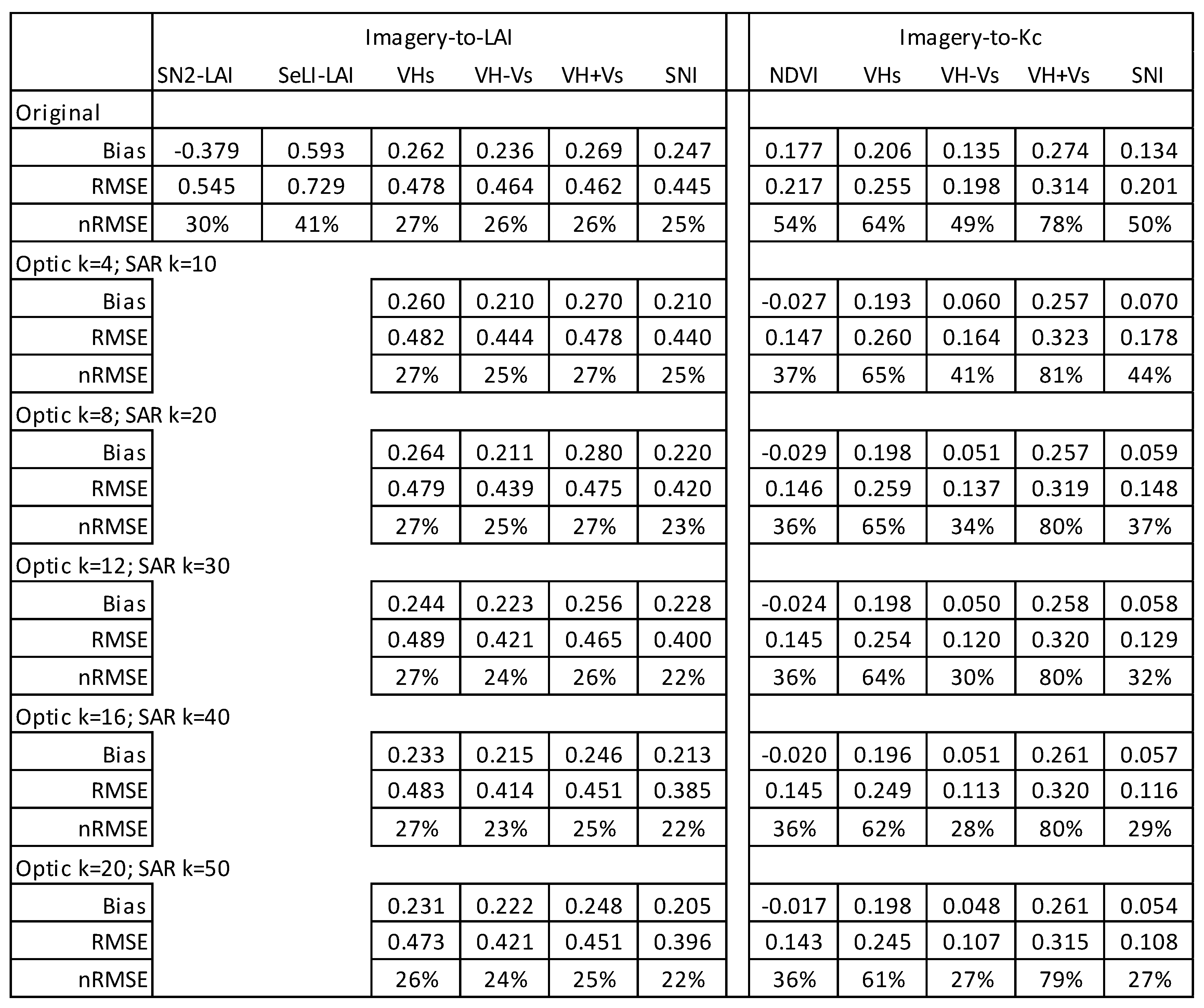
The RMSE values for the four SAR indices (
Table 2) reveal different patterns. First, for two indices, scaled_VH and scaled_VH + VV, our approach did not reduce the RMSE. Yet, for the other two, scaled_VH − VV and SNI, this procedure improved the accuracy from 0.20 to 0.11 (
k = 50).
To increase the amount of data available to estimate Kc, we integrated each of the two SAR indices with the optic NDVI. The integration included different
k values for each source. We tried three sets of
k: 50, 30; 20, 12; and 20, 12 for the SAR, optic and fused data, respectively. The results indicate reduced RMSE values (
Table 3), but also that lower
k values (30 for SAR and 12 for NDVI) yield slightly better accuracy. This may indicate that the fusion of the two datasets, SAR and optic, generates a new set, and we therefore require a set of
k for SAR and optic and different
k for the fused series.
The indices corresponding to the lowest RMSE were plotted against the estimated K
c from the LAI field measurements (
Figure 5). This outlines not only the improvement in the R
2 for the fused data, but also an increase in the number of observations (i.e., higher temporal resolution) because of the combination of different sources.
3.2. LAI Estimations by Satellite Imagery
The LAI estimations by satellite imagery are based on the 27 dates (30% of the S1 data) that were used for the validation of S1 (§2.5 LAI estimations). The RMSE of the LAI estimations by satellite imagery are summarized in
Table 4.
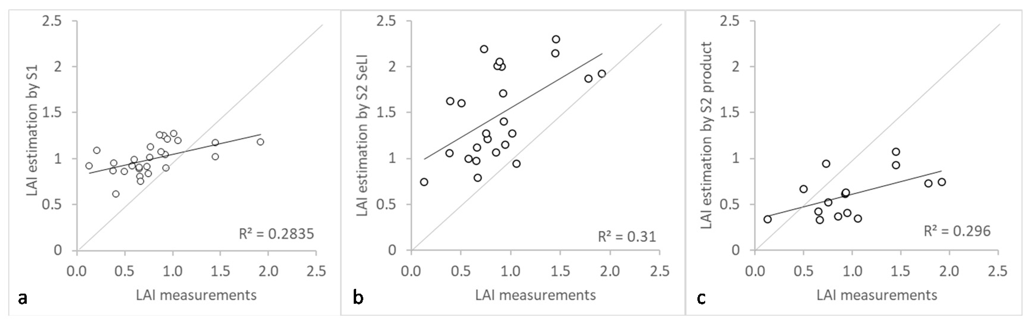
The RMSE of S2, determined either by the biophysical product (SN2-LAI) or the SeLI, is higher than that of S1, even when considering the original values. However, the range of our LAI measurements is small, and therefore the nRMSE for the SAR indices is 26–27%, while [
26] reported an nRMSE of 14% for the SeLI product. Furthermore, as most of the LAI measurements in our dataset are below 2.0, the accuracy of the LAI from the optical satellite imagery should be low, as presented elsewhere [
27].
The advantages of S1 estimations are further outlined in the scatter plots of the SNI (with
k = 40), the S2 SeLI, and the S2 LAI product (
Figure 6). While the SeLI over-estimates, especially in low LAI values (<1.0), which occurred at the beginning of the season, and the S2 LAI product under-estimates, the SNI is more close to the 1:1 line, resulting in an RMSE that is much better for the SAR estimations.
4. Discussion
The resulting RMSE values for both Kc and LAI are aligned with published RMSE values. The Kc-RMSE of the NDVI, scaled_VH-HH and the SNI (<0.145), achieved using our approach, are comparable to the RMSE values found by [
22] (0.08–0.09), [
28] (0.16–0.19), [
29] (0.14–0.17), and [
30] (0.04–0.30). The LAI-RMSE of the SNI (RMSE = 0.385, nRMSE = 22%) is in the range of RMSE values found by others: 0.30 for orchards by Landsat-7 [
31], 0.98 and 1.63 for field crops by S2 and L8, respectively [
32], 1.11 and 0.69 for orchards and field crops by the S2 LAI product and the SeLI estimations, respectively [
26], and 2.26 with an nRMSE of 52% for field crops by S2 [
33].
Our approach achieved this accuracy by reducing the RMSE by 30–45% for the Kc and 10–13% for the LAI, compared to the original values. This improved accuracy, either for optic or for the SAR, outlines the importance of this temporal smoothing (without the need for spatial smoothing) that preserves the original GSD of 10 m. It means that our approach generalizes better, as it applies to small-size plots (as well as large plots). To be more specific, when considering spatial smoothing (especially in SAR data), there are two methods: one that changes the size of the pixels (e.g., multilooking [
34]) and one that does not change the pixel size (e.g., low pass filter), a more “traditional” one in that sense. We decided not to perform the former because we wanted to keep the original 10 m GSD due to the size of our small plots (see plot dimensions in
Figure 1). For that reason, we also decided not to apply the latter, because we did not want any influence from the adjacent pixels that are not part of the plot. One can argue that we could mask the pixels outside of the plots, but due to their size, the spatial smoothing effect will be negligible. As such, our approach applies to both large and small plots, whereas spatial smoothing will demand plots of minimum size.
The RMSE values of the scaled_VH-VV and the SNI (for
k ≥ 30) (
Table 2) are better (lower) than optic’s RMSE (
Table 1). This can be attributed to the double-bounce effect of the SAR, which is sensitive to the geometry of the crop, enabling us to better estimate the volume of the vine plants as compared to the optic data [
35].
The better accuracy of these two SAR indices, together with the presence of more imagery for the same time frame (88 vs. 47 for SAR and optic, respectively), promotes using them as a surrogate source of optic data for irrigation monitoring. Further, the frequency of the SAR images, which in our dataset was every 2–3 days, is better than the irrigation decision-making requirement of once-a-week. Therefore, the quantity and the accuracy of the SAR data make them an exceptional source for this target.
The fusing of the SAR and optic achieved similar results to the SAR (0.1 vs. 0.107). In that sense, the combination of optical and SAR images did not much improve the results. Nevertheless, we developed this approach so it can be generalized to other vineyards with different row structures, canopy covers, and potentially other crops. The fact that, in this particular study, the optic did not “interrupt” the superiority of the SAR in estimating Kc and LAI proves that our approach is robust and can be applied to other plots. Certainly, further study is needed.
5. Conclusions
In this study, we presented an approach to estimate Kc and LAI from both SAR and optic satellite imagery. Our approach is relatively simple and scalable, as it does not require a huge dataset and does not need to process large images.
Our results indicate that SAR can estimate Kc and LAI as effectively as optic imagery and, in some cases, achieve even better accuracy. Therefore, we conclude that Sentinel-1 can serve as a valid alternative to optic data for Kc and LAI estimation for vineyards, which is especially important in an area with moderate and heavy cloud cover.
The better accuracy of the SAR indices (in some cases), compared to the NDVI, may be related to the small percentage of the crop in each pixel, which might have less of an influence on the SAR backscattering. From the SAR indices we tested, the results of the SNI were slightly better than those of the VH-VV, which makes the SNI favorable for future applications.
Additionally, the integration of the optic and the SAR not only gave better results, but also ensured a value at least once a week, which is an invaluable factor for irrigation decision-making.
This study opens the door for further work, such as utilizing data from the same plots with time-series analysis or artificial intelligence, in order to better estimate Kc and LAI for vineyards.
Author Contributions
Conceptualization, O.B., A.H. and Y.N.; methodology, O.B. and R.P.; resources, Y.N., S.M. and D.F.M.; writing—original draft preparation, O.B. and R.P.; writing—review and editing, T.S. and Y.N.; supervision, S.M.-t. All authors have read and agreed to the published version of the manuscript.
Funding
This study was sponsored by the Ministry of Science and Technology (Grant No. 6-6802), Israel, the Ministry of Agriculture and Rural Development (Grants No. 31-01-0013, 31-01-0010), Israel and the Israeli Wine Grape Council.
Acknowledgments
The authors would like to thank the dedicated growers: Moshe Hernik, Yoav David, Itamar Weis, Yedidia Maman and Shlomi Coh en. We thank Yechezkel Harroch, Bentzi Green, Yossi Shteren, Alon Katz, Ben Hazut, Elnatan Golan, David Kimchi, Gilad Gersman, Yedidia Sweid, and Yair Hayat for assisting in the field measurements. The authors greatly appreciate three anonymous reviewers for their important comments.
Conflicts of Interest
The authors declare no conflict of interest.
Appendix A
Table A1.
LAI measurement dates and corresponding satellite imagery.
Table A1.
LAI measurement dates and corresponding satellite imagery.
| South Plot | North Plot |
|---|
| Measurement | Sentinel-1 | Optic | Measurement | Sentinel-1 | Optic |
|---|
| 26-Apr-2016 | 27-Apr-2016 | | 23-Apr-2017 | 22-Apr-2017 | |
| 16-May-2016 | 17-May-2016 | | 30-Apr-2017 | 30-Apr-2017 | |
| 13-Jun-2016 | 14-Jun-2016 | | 7-May-2017 | 6-May-2017 | |
| 4-Jul-2016 | 4-Jul-2016 | | 14-May-2017 | 12-May-2017 | 12-May-2017 |
| 18-Jul-2016 | 20-Jul-2016 | | 28-May-2017 | 28-May-2017 | 28-May-2017 |
| 1-Aug-2016 | 1-Aug-2016 | | 4-Jun-2017 | 4-Jun-2017 | |
| 9-Aug-2016 | 9-Aug-2016 | | 11-Jun-2017 | 11-Jun-2017 | 10-Jun-2017 |
| 15-Aug-2016 | 13-Aug-2016 | 13-Aug-2016 | 25-Jun-2017 | 23-Jun-2017 | |
| 22-Aug-2016 | 21-Aug-2016 | | 9-Jul-2017 | 9-Jul-2017 | 10-Jul-2017 |
| 19-Apr-2017 | 18-Apr-2017 | | 30-Jul-2017 | 29-Jul-2017 | 30-Jul-2017 |
| 27-Apr-2017 | 28-Apr-2017 | 26-Apr-2017 | 8-Apr-2018 | 7-Apr-2018 | |
| 10-May-2017 | 10-May-2017 | | 15-Apr-2018 | 13-Apr-2018 | 13-Apr-2018 |
| 17-May-2017 | 16-May-2017 | | 29-Apr-2018 | 29-Apr-2018 | 29-Apr-2018 |
| 25-May-2017 | 24-May-2017 | | 18-May-2018 | 18-May-2018 | |
| 7-Jun-2017 | 5-Jun-2017 | | 27-May-2018 | 25-May-2018 | |
| 15-Jun-2017 | 15-Jun-2017 | 13-Jun-2017 | 10-Jun-2018 | 10-Jun-2018 | 10-Jun-2018 |
| 28-Jun-2017 | 28-Jun-2017 | | 17-Jun-2018 | 17-Jun-2018 | 16-Jun-2018 |
| 5-Jul-2017 | 5-Jul-2017 | | 24-Jun-2018 | 24-Jun-2018 | |
| 12-Jul-2017 | 11-Jul-2017 | 10-Jul-2017 | 8-Jul-2018 | 10-Jul-2018 | 10-Jul-2018 |
| 18-Jul-2017 | 17-Jul-2017 | | 22-Jul-2018 | 22-Jul-2018 | 20-Jul-2018 |
| 27-Jul-2017 | 27-Jul-2017 | | 14-May-2019 | 14-May-2019 | 16-May-2019 |
| 2-Aug-2017 | 3-Aug-2017 | | 21-May-2019 | 20-May-2019 | 21-May-2019 |
| 17-Aug-2017 | 16-Aug-2017 | 16-Aug-2017 | 28-May-2019 | 26-May-2019 | 26-May-2019 |
| 23-Aug-2017 | 22-Aug-2017 | | 4-Jun-2019 | 5-Jun-2019 | 3-Jun-2019 |
| 30-Aug-2017 | 28-Aug-2017 | | 11-Jun-2019 | 11-Jun-2019 | 10-Jun-2019 |
| 6-Sep-2017 | 7-Sep-2017 | | 18-Jun-2019 | 18-Jun-2019 | |
| 16-Apr-2018 | 17-Apr-2018 | | 25-Jun-2019 | 25-Jun-2019 | 25-Jun-2019 |
| 30-Apr-2018 | 30-Apr-2018 | 29-Apr-2018 | 2-Jul-2019 | 1-Jul-2019 | 30-Jun-2019 |
| 21-May-2018 | 19-May-2018 | | 9-Jul-2019 | 7-Jul-2019 | |
| 4-Jun-2018 | 4-Jun-2018 | | 16-Jul-2019 | 17-Jul-2019 | |
| 11-Jun-2018 | 11-Jun-2018 | 10-Jun-2018 | 30-Jul-2019 | 30-Jul-2019 | 30-Jul-2019 |
| 18-Jun-2018 | 18-Jun-2018 | | 6-Aug-2019 | 6-Aug-2019 | 6-Aug-2019 |
| 25-Jun-2018 | 24-Jun-2018 | | 13-Aug-2019 | 12-Aug-2019 | 14-Aug-2019 |
| 2-Jul-2018 | 30-Jun-2018 | 30-Jun-2018 | 3-Sep-2019 | 3-Sep-2019 | 3-Sep-2019 |
| 9-Jul-2018 | 10-Jul-2018 | 10-Jul-2018 | 10-Sep-2019 | 10-Sep-2019 | |
| 16-Jul-2018 | 16-Jul-2018 | 15-Jul-2018 | 24-Sep-2019 | 23-Sep-2019 | 23-Sep-2019 |
| 23-Jul-2018 | 22-Jul-2018 | | | | |
| 30-Jul-2018 | 29-Jul-2018 | | | | |
| 20-Aug-2018 | 19-Aug-2018 | | | | |
| 29-Apr-2019 | 30-Apr-2019 | | | | |
| 13-May-2019 | 13-May-2019 | 11-May-2019 | | | |
| 20-May-2019 | 20-May-2019 | 18-May-2019 | | | |
| 27-May-2019 | 26-May-2019 | 26-May-2019 | | | |
| 3-Jun-2019 | 5-Jun-2019 | 3-Jun-2019 | | | |
| 10-Jun-2019 | 11-Jun-2019 | 10-Jun-2019 | | | |
| 17-Jun-2019 | 17-Jun-2019 | | | | |
| 24-Jun-2019 | 24-Jun-2019 | | | | |
| 1-Jul-2019 | 1-Jul-2019 | 30-Jun-2019 | | | |
| 8-Jul-2019 | 7-Jul-2019 | 5-Jul-2019 | | | |
| 15-Jul-2019 | 17-Jul-2019 | | | | |
| 5-Aug-2019 | 5-Aug-2019 | 4-Aug-2019 | | | |
| 9-Sep-2019 | 9-Sep-2019 | 7-Sep-2019 | | | |
| 23-Sep-2019 | 23-Sep-2019 | 23-Sep-2019 | | | |
Figure A1.
Accuracy metric statistics (Bias, RMSE, and nRMSE).
Figure A1.
Accuracy metric statistics (Bias, RMSE, and nRMSE).
Appendix B
Figure A2a,b show a typical behavior of SAR and NDVI values during a growing season, where on the one hand SAR exhibits more data points as it is not affected by clouds, and on the other hand, it is noisier than the optic thus a more “strict” smooth (higher value of
k) is needed for the SAR data.
To determine the minimum and maximum values for each Equations (4)–(7), we utilized the following process, which can be found elsewhere [
36].
We downloaded a time-series of VH and VV from GEE for different locations, land covers, and crops. It includes data over groundnuts, corn, cotton, processing-tomato, almonds, olives, apples, pomegranate, forest and bare soil in Israel; alfalfa and pistachio in the United-State; coffee and soybean in Brazil; potatoes in Turkey; cotton in Australia; sugarcane in Nicaragua and processing-tomatoes in Italy. The timeframe for each location was around a yearlong to ensure SAR data for all growth periods and field stages such as bare soil, crop development stage, and full vegetation cover.
Using this data, we determined the minimum and maximum values for the VH and VV. We then plugged-in the minimum and maximum values (separately) for each of the Equations (4)–(6) and determined the scaling factors (i.e.,
f1–f5) so that the index values will range between 0.0 and 1.0 to fit the 0.0–1.0 range of NDVI values for agriculture plots. Even though the indices values were between 0.0 and 1.0 (considering the minimum and maximum values), the indices values during the growing season have a narrower range, approximately between 0.2 and 0.8. (
Figure A2c, orange curve).
As mentioned in
Section 2.4.2, we wanted to calculate NDVI-like for the SAR data and to bring both NDVI and NDVI
SAR to the same values range. To that end, we applied a stretching function (Equation (9)) (for both) featuring minimum and maximum values that were determined in a similar way to the scaling factors (
Figure A2c, blue curve).
Figure A2.
Remote sensing data for 2019 over the north plot. (a)—Sentinel-1 backscatter values (dB) of VV and VH, (b)—NDVI values, and (c)—scaled_VH index (Equation (4)) before (orange) and after (blue) stretch (Equation (9)). Note that VV and VH (a) are noisier than the NDVI (b) but also include many more data points. Please also note the stretch effect (c) where the index values are closer to the desired range (0–1) after the stretch.
References
- Allen, R.G.; Pereira, L.S.; Raes, D.; Smith, M. FAO Irrigation and Drainage Paper No 56: Crop. Evapotranspiration; FAO: Rome, Italy, 1998. [Google Scholar]
- Ohana-Levi, N.; Munitz, S.; Ben-Gal, A.; Schwartz, A.; Peeters, A.; Netzer, Y. Multiseasonal grapevine water consumption—Drivers and forecasting. Agric. For. Meteorol. 2020, 280, 107796. [Google Scholar] [CrossRef]
- Ohana-Levi, N.; Munitz, S.; Ben-Gal, A.; Netzer, Y. Evaluation of within-season grapevine evapotranspiration patterns and drivers using generalized additive models. Agric. Water Manag. 2020, 228, 105808. [Google Scholar] [CrossRef]
- Netzer, Y.; Yao, C.; Shenker, M.; Bravdo, B.A.; Schwartz, A. Water use and the development of seasonal crop coefficients for Superior Seedless grapevines trained to an open-gable trellis system. Irrig. Sci. 2009, 27, 109–120. [Google Scholar] [CrossRef]
- Masahiro, T.; Allen, R.G.; Trezza, R. Calibrating satellite-based vegetation indices to estimate evapotranspiration and crop coefficients. In Proceedings of the Ground Water and Surface Water Under Stress: Competition, Interaction, Solution, Boise, Idaho, 25–28 October 2006; pp. 103–112. [Google Scholar]
- Johnson, L.F.; Trout, T.J. Satellite NDVI assisted monitoring of vegetable crop evapotranspiration in california’s san Joaquin Valley. Remote Sens. 2012, 4, 439–455. [Google Scholar] [CrossRef] [Green Version]
- Nagler, P.L.; Glenn, E.P.; Nguyen, U.; Scott, R.L.; Doody, T. Estimating riparian and agricultural actual evapotranspiration by reference evapotranspiration and MODIS enhanced vegetation index. Remote Sens. 2013, 5, 3849–3871. [Google Scholar] [CrossRef] [Green Version]
- Brown, S.C.M.; Quegan, S.; Morrison, K.; Bennett, J.C.; Cookmartin, G. High-resolution measurements of scattering in wheat canopies—Implications for crop parameter retrieval. IEEE Trans. Geosci. Remote Sens. 2003, 41, 1602–1610. [Google Scholar] [CrossRef] [Green Version]
- Macelloni, G.; Paloscia, S.; Pampaloni, P.; Marliani, F.; Gai, M. The relationship between the backscattering coefficient and the biomass of narrow and broad leaf crops. IEEE Trans. Geosci. Remote Sens. 2001, 39, 873–884. [Google Scholar] [CrossRef]
- Torbick, N.; Chowdhury, D.; Salas, W.; Qi, J. Monitoring Rice Agriculture across Myanmar Using Time Series Sentinel-1 Assisted by Landsat-8 and PALSAR-2. Remote Sens. 2017, 9, 119. [Google Scholar] [CrossRef] [Green Version]
- Gao, Q.; Zribi, M.; Escorihuela, M.J.; Baghdadi, N. Synergetic use of sentinel-1 and sentinel-2 data for soil moisture mapping at 100 m resolution. Sensors 2017, 17, 1966. [Google Scholar] [CrossRef] [PubMed] [Green Version]
- Attarzadeh, R.; Amini, J.; Notarnicola, C.; Greifeneder, F. Synergetic use of Sentinel-1 and Sentinel-2 data for soil moisture mapping at plot scale. Remote Sens. 2018, 10, 1285. [Google Scholar] [CrossRef] [Green Version]
- Rusmini, M.; Candiani, G.; Frassy, F.; Maianti, P.; Marchesi, A.; Nodari, F.R.; Dini, L.; Gianinetto, M. High resolution SAR and high resolution optical data integration for sub-urban land cover classification. In Proceedings of the 2012 IEEE International Geoscience and Remote Sensing Symposium, Munich, Germany, 22–27 July 2012; pp. 4986–4989. [Google Scholar] [CrossRef]
- Forkuor, G.; Conrad, C.; Thiel, M.; Ullmann, T.; Zoungrana, E. Integration of optical and synthetic aperture radar imagery for improving crop mapping in northwestern Benin, West Africa. Remote Sens. 2014, 6, 6472–6499. [Google Scholar] [CrossRef] [Green Version]
- Pratola, C.; Lcciardi, G.A.; Del Frate, F.; Schiavon, G.; Solimini, D. Fusion of VHR multispectral and X-band SAR data for the enhancement of vegetation maps. In Proceedings of the 2012 IEEE International Geoscience and Remote Sensing Symposium, Munich, Germany, 22–27 July 2012; pp. 6793–6796. [Google Scholar] [CrossRef]
- Navarro, A.; Rolim, J.; Miguel, I.; Catalão, J.; Silva, J.; Painho, M.; Vekerdy, Z. Crop monitoring based on SPOT-5 Take-5 and sentinel-1A data for the estimation of crop water requirements. Remote Sens. 2016, 8, 525. [Google Scholar] [CrossRef] [Green Version]
- Moran, M.S.; Hymer, D.C.; Qi, J.; Kerr, Y. Comparison of ers-2 sar and landsat tm imagery for monitoring agricultural crop and soil conditions. Remote Sens. Environ. 2002, 79, 243–252. [Google Scholar] [CrossRef]
- Filgueiras, R.; Mantovani, E.C.; Althoff, D.; Fernandes Filho, E.I.; da Cunha, F.F. Crop NDVI monitoring based on sentinel 1. Remote Sens. 2019, 11, 1441. [Google Scholar] [CrossRef] [Green Version]
- Munitz, S.; Schwartz, A.; Netzer, Y. Effect of timing of irrigation initiation on vegetative growth, physiology and yield parameters in Cabernet Sauvignon grapevines. Aust. J. Grape Wine Res. 2020, 26, 220–232. [Google Scholar] [CrossRef]
- Munitz, S.; Schwartz, A.; Netzer, Y. Water consumption, crop coefficient and leaf area relations of a Vitis vinifera cv. “Cabernet Sauvignon” vineyard. Agric. Water Manag. 2019, 219, 86–94. [Google Scholar] [CrossRef]
- Allen, R.G.; Pereira, L.S. Estimating crop coefficients from fraction of ground cover and height. Irrig. Sci. 2009, 28, 17–34. [Google Scholar] [CrossRef] [Green Version]
- Beeri, O.; Pelta, R.; Shilo, T.; Mey-tal, S.; Tanny, J. Accuracy of crop coefficient estimation methods based on satellite imagery. In Precision Agriculture’19; Stafford, J.V., Ed.; Wageningen Academic Publishers: Wageningen, The Netherlands, 2019; pp. 437–444. [Google Scholar]
- Gillies, R.R.; Carlson, T.N. Thermal Remote Sensing of Surface Soil Water Content with Partial Vegetation Cover for Incorporation into Climate Models. J. Appl. Meteorol. 1995, 34, 745–756. [Google Scholar] [CrossRef] [Green Version]
- Atkeson, C.; Moore, W.; Schaal, S. Locally Weighted Learning. In Lazy Learning; Aha, D.W., Ed.; Springer: Dordrecht, The Netherlands, 1997. [Google Scholar]
- Fieuzal, R.; Baup, F.; Marais-Sicre, C. Monitoring Wheat and Rapeseed by Using Synchronous Optical and Radar Satellite Data—From Temporal Signatures to Crop Parameters Estimation. Adv. Remote Sens. 2013, 2, 162–180. [Google Scholar] [CrossRef] [Green Version]
- Pasqualotto, N.; Delegido, J.; Van Wittenberghe, S.; Rinaldi, M.; Moreno, J. Multi-crop green LAI estimation with a new simple sentinel-2 LAI index (SeLI). Sensors 2019, 19, 904. [Google Scholar] [CrossRef] [Green Version]
- Vuolo, F.; Zóltak, M.; Pipitone, C.; Zappa, L.; Wenng, H.; Immitzer, M.; Weiss, M.; Baret, F.; Atzberger, C. Data service platform for Sentinel-2 surface reflectance and value-added products: System use and examples. Remote Sens. 2016, 8, 938. [Google Scholar] [CrossRef] [Green Version]
- Kamble, B.; Kilic, A.; Hubbard, K. Estimating crop coefficients using remote sensing-based vegetation index. Remote Sens. 2013, 5, 1588–1602. [Google Scholar] [CrossRef] [Green Version]
- Park, J.; Baik, J.; Choi, M. Satellite-based crop coefficient and evapotranspiration using surface soil moisture and vegetation indices in Northeast Asia. Catena 2017, 156, 305–314. [Google Scholar] [CrossRef]
- Pôças, I.; Paço, T.A.; Paredes, P.; Cunha, M.; Pereira, L.S. Estimation of actual crop coefficients using remotely sensed vegetation indices and soil water balance modelled data. Remote Sens. 2015, 7, 2373–2400. [Google Scholar] [CrossRef] [Green Version]
- Zarate-valdez, J.L.; Whiting, M.L.; Lampinen, B.D.; Metcalf, S.; Ustin, S.L.; Brown, P.H. Prediction of leaf area index in almonds by vegetation indexes. Comput. Electron. Agric. 2012, 85, 24–32. [Google Scholar] [CrossRef]
- Djamai, N.; Fernandes, R.; Weiss, M.; McNairn, H.; Goïta, K. Validation of the Sentinel Simplified Level 2 Product Prototype Processor (SL2P) for mapping cropland biophysical variables using Sentinel-2/MSI and Landsat-8/OLI data. Remote Sens. Environ. 2019, 225, 416–430. [Google Scholar] [CrossRef]
- Kganyago, M.; Mhangara, P.; Alexandridis, T.; Laneve, G.; Ovakoglou, G.; Mashiyi, N. Validation of sentinel-2 leaf area index (LAI) product derived from SNAP toolbox and its comparison with global LAI products in an African semi-arid agricultural landscape. Remote Sens. Lett. 2020, 11, 883–892. [Google Scholar] [CrossRef]
- Raney, K. Radar fundamentals: Technical prespective. In Principles and Application of Imaging Radar; Manual of Remote Sensing; Henderson, F., Lewis, A., Eds.; John Wiley & Suns Inc.: New York, NY, USA, 1998; Volume 2, pp. 9–129. [Google Scholar]
- Patel, P.; Srivstava, H.S.; Panigtahy, S.; Parihar, J.S. Comparative evaluation of the sensitivity of multi-polarized multi-frequency SAR backscatter to plant density. Int. J. Remote Sens. 2006, 27, 293–305. [Google Scholar] [CrossRef]
- Wagner, W.; Lemoine, G.; Rott, H. A method for estimating soil moisture from ERS Scatterometer and soil data. Remote Sens. Environ. 1999, 70, 191–207. [Google Scholar] [CrossRef]
Figure 1.
The study area—two vineyard plots in Israel. Upper images—the north plot, lower images—the south plot. Data from the center six sub-plots (marked in red) were used in this study. The dimensions of each plot and sub-plot are 120 × 36 m and 24 × 9 m, respectively. The base map is the Google Satellite Hybrid in QGIS. The plot photos were taken by Y. Netzer.
Figure 2.
LAI measurements at each plot (north and south) for each growing season. Errors bars represent standard error.
Figure 2.
LAI measurements at each plot (north and south) for each growing season. Errors bars represent standard error.
Figure 3.
Kc estimation flowchart. Starting by preprocessing all images, calculate NDVI, then stretch and smooth NDVI values using locally weighted regression. The output is three estimations of Kc, namely from the optic, the SAR, and a fused Kc. Note that NDVISAR refers to all indices in Equations (4)–(7).
Figure 4.
LAI estimation workflow. We calculated LAI using remote sensing data via three methods, namely LAISeLI, LAISNAP and LAISAR. The Sentinel-1 dataset was split into train and test set, and the evaluation of all three methods was performed against the test set.
Figure 4.
LAI estimation workflow. We calculated LAI using remote sensing data via three methods, namely LAISeLI, LAISNAP and LAISAR. The Sentinel-1 dataset was split into train and test set, and the evaluation of all three methods was performed against the test set.
Figure 5.
Kc estimation (from LAI measurements) versus satellite Kc estimations. (a) SNI (n = 89, k = 50); (b) NDVI (n = 42, k = 20); (c) Fused (n = 89, k = 20). Gray line represents 1:1 line.
Figure 5.
Kc estimation (from LAI measurements) versus satellite Kc estimations. (a) SNI (n = 89, k = 50); (b) NDVI (n = 42, k = 20); (c) Fused (n = 89, k = 20). Gray line represents 1:1 line.
Figure 6.
LAI measurements versus satellite estimations. (a) Sentinel-1 SNI (n = 29, k = 40); (b) Sentinel-2 SeLI (n = 25); (c) Sentinel-2 product from SNAP (n = 15). Gray line represents 1:1 line.
Figure 6.
LAI measurements versus satellite estimations. (a) Sentinel-1 SNI (n = 29, k = 40); (b) Sentinel-2 SeLI (n = 25); (c) Sentinel-2 product from SNAP (n = 15). Gray line represents 1:1 line.
Table 1.
Root-mean-square-error (RMSE) of the normalized difference vegetation index (NDVI) for the original values and different k values (n = 47).
Table 1.
Root-mean-square-error (RMSE) of the normalized difference vegetation index (NDVI) for the original values and different k values (n = 47).
| | Original Values | k = 4 | k = 8 | k = 12 | k = 16 | k = 20 |
|---|
| NDVI | 0.217 | 0.147 | 0.146 | 0.145 | 0.145 | 0.143 |
Table 2.
RMSE of the SAR indices for the original values and different k values (n = 88).
Table 2.
RMSE of the SAR indices for the original values and different k values (n = 88).
| | Original Values | k = 10 | k = 20 | k = 30 | k = 40 | k = 50 |
|---|
| scaled_VH | 0.255 | 0.260 | 0.259 | 0.254 | 0.249 | 0.245 |
| scaled_VH − VV | 0.198 | 0.164 | 0.137 | 0.120 | 0.113 | 0.107 |
| scaled_VH + VV | 0.314 | 0.323 | 0.319 | 0.320 | 0.320 | 0.315 |
| SNI | 0.201 | 0.178 | 0.148 | 0.129 | 0.116 | 0.108 |
Table 3.
RMSE of the fused SAR indices (scaled_VH − VV and SNI) and optic NDVI, with different k values for fused (n = 88).
Table 3.
RMSE of the fused SAR indices (scaled_VH − VV and SNI) and optic NDVI, with different k values for fused (n = 88).
| | SAR (k = 50), Optic (k = 20), Fused (k = 20) | SAR (k = 30), Optic (k = 12), Fused (k = 12) |
|---|
| NDVI + scaled_VH − VV | 0.102 | 0.100 |
| NDVI + SNI | 0.101 | 0.098 |
Table 4.
RMSE of the optic (n = 25) and SAR (n = 27) indices for LAI estimation.
Table 4.
RMSE of the optic (n = 25) and SAR (n = 27) indices for LAI estimation.
| | Original Values | k = 10 | k = 20 | k = 30 | k = 40 | k = 50 |
|---|
| Sentinel-2 LAI | 0.490 | | | | | |
| Sentinel-2 SeLI | 0.690 | | | | | |
| scaled_VH | 0.478 | 0.482 | 0.479 | 0.489 | 0.483 | 0.473 |
| scaled_VH − VV | 0.464 | 0.444 | 0.439 | 0.421 | 0.414 | 0.421 |
| scaled_VH + VV | 0.462 | 0.478 | 0.475 | 0.465 | 0.451 | 0.451 |
| SNI | 0.445 | 0.440 | 0.420 | 0.400 | 0.385 | 0.396 |
| Publisher’s Note: MDPI stays neutral with regard to jurisdictional claims in published maps and institutional affiliations. |
© 2020 by the authors. Licensee MDPI, Basel, Switzerland. This article is an open access article distributed under the terms and conditions of the Creative Commons Attribution (CC BY) license (http://creativecommons.org/licenses/by/4.0/).

 ,
, 


