Vertical Accuracy of Freely Available Global Digital Elevation Models (ASTER, AW3D30, MERIT, TanDEM-X, SRTM, and NASADEM)

Abstract

Freely available global digital elevation models (DEMs) are important inputs for many research fields and applications. During the last decade, several global DEMs have been released based on satellite data. ASTER and SRTM are the most widely used DEMs, but the more recently released, AW3D30, TanDEM-X and MERIT, are being increasingly used. Many researchers have studied the quality of these DEM products in recent years. However, there has been no comprehensive and systematic evaluation of their quality over areas with variable topography and land cover conditions. To provide this comparison, we examined the accuracy of six freely available global DEMs (ASTER, AW3D30, MERIT, TanDEM-X, SRTM, and NASADEM) in four geographic regions with different topographic and land use conditions. We used local high-precision elevation models (Light Detection and Ranging (LiDAR), Pleiades-1A) as reference models and all global models were resampled to reference model resolution (1m). In total, 608 million 1x1 m pixels were analyzed. To estimate the accuracy, we generated error rasters by subtracting each reference model from the corresponding global DEM and calculated descriptive statistics for this difference (e.g., median, mean, root-mean-square error (RMSE)). We also assessed the vertical accuracy as a function of the slope, slope aspect, and land cover. We found that slope had the strongest effect on DEM accuracy, with no relationship for slope aspect. The AW3D30 was the most robust and had the most stable performance in most of the tests and is therefore the best choice for an analysis of multiple geographic regions. SRTM and NASADEM also performed well where available, whereas NASADEM, as a successor of SRTM, showed only slight improvement in comparison to SRTM. MERIT and TanDEM-X also performed well despite their lower spatial resolution.

1. Introduction

Digital elevation models (DEMs) and the topographic and terrain variables derived from these models (e.g., slope aspect, slope, channels, hillslopes) are fundamental inputs for environmental and landscape modeling and spatial analysis [1,2,3,4,5], especially for research in geomorphology [6], hydrology [7], and geology [8]. For several decades, DEM products have been created at different spatial scales (e.g., global or national) mainly using remote sensing data [9]. As different remote sensing data and methods are employed during the development of DEMs, it has become increasingly important to assess the accuracy and performance of such products to provide insights into their limitations [10] and develop correction procedures [11,12]. The potential artifacts (errors) and inconsistencies identified in DEM products usually arise from distortions caused by atmospheric, terrain, and sensor conditions at the moment of the data acquisition [10,13,14].

Due to the potential analytical bias that results from artifacts and inconsistencies in DEMs, several studies have investigated the quality of such products, especially for those developed at a global scale. These investigations usually focused on the height (vertical) accuracy of the DEM [15,16] or the model’s performance in different applications, such as river network generation, the acquisition of geomorphological metrics, and flood simulation [12,17]. Most of the assessments compare freely available DEM products with GPS survey points [18] or with DEMs developed based on photogrammetric aerial images or on laser scanning (e.g., LiDAR) [19]. For instance, the vertical accuracy of the Shuttle Radar Topography Mission (SRTM; released in 2003) ranges from 2.18 to 21.70 m [10,20] and for the Advanced Spaceborne Thermal Emission and Reflection satellite (ASTER, released in 2006), the accuracy ranges from 4.56 to 7.10 m [10,20]. These high-resolution global DEM products, developed based on radar data (SRTM) and data from optical sensors (ASTER), were one of the first freely available DEMs at a global scale. Recently, new freely available global-scale DEM products have been released, such as the TanDEM-X DEM [15], the Multi-Error-Removed Improved-Terrain (MERIT) DEM [21], the ALOS Global Digital Surface Model (AW3D30) [22], and the NASADEM [23]. Because these products are so new (TanDEM-X has been freely available since late 2018, MERIT 2017, AW3D30 and NASADEM since the beginning of 2020), fewer studies have evaluated their accuracy [24,25,26,27,28]. If their accuracy can be confirmed, these new DEM products, which are based on more current remote sensing data and better processing methods, will be highly valuable because of their ability to capture natural or man-made changes in the topography of terrestrial surfaces [29].

DEM products are continuously being improved, and new versions are being released constantly. Usually, the newest versions are developed by applying analytical improvements that reduce errors or inconsistencies identified in the previous DEM versions, especially based on assessment studies [9,30]. Many researchers have assessed the quality of the global-scale DEM products in recent years [26,28,30]. However, there has been no comprehensive and systematic evaluation of the quality of these freely available global DEMs over areas with variable topography and land cover conditions. The accuracy of the DEMs can largely vary depending on the latitude, vegetation, and topography. In addition, previous studies have only used a few hundred GPS points for ground control [30,31] or LiDAR-based DEM averaged to global DEM resolution [26] which results in a loss of information. In our study, we evaluated the performance of the freely available DEM products (ASTER, AW3D30, MERIT, TanDEM-X, SRTM, and NASADEM) in four different regions of the world with different topography and land cover characteristics. We used locally derived LiDAR-based DEMs and the Pleiades 1A data as reference models to estimate the accuracy and resampled all the global models to the reference model resolution (1 m) which resulted in a total of 608 million 1x1 m pixels. This enabled us to perform the accuracy assessment at the highest possible resolution (1 m) and capture the continuous nature of topography. We estimated the vertical accuracy of the global DEM products as a function of slope, slope aspect, and land cover type. To the best of our knowledge, the accuracy of NASADEM has not been systematically estimated before against ground truth and in comparison with SRTM.

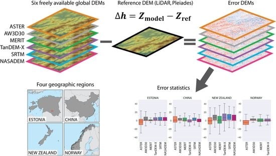
2. Materials and Methods

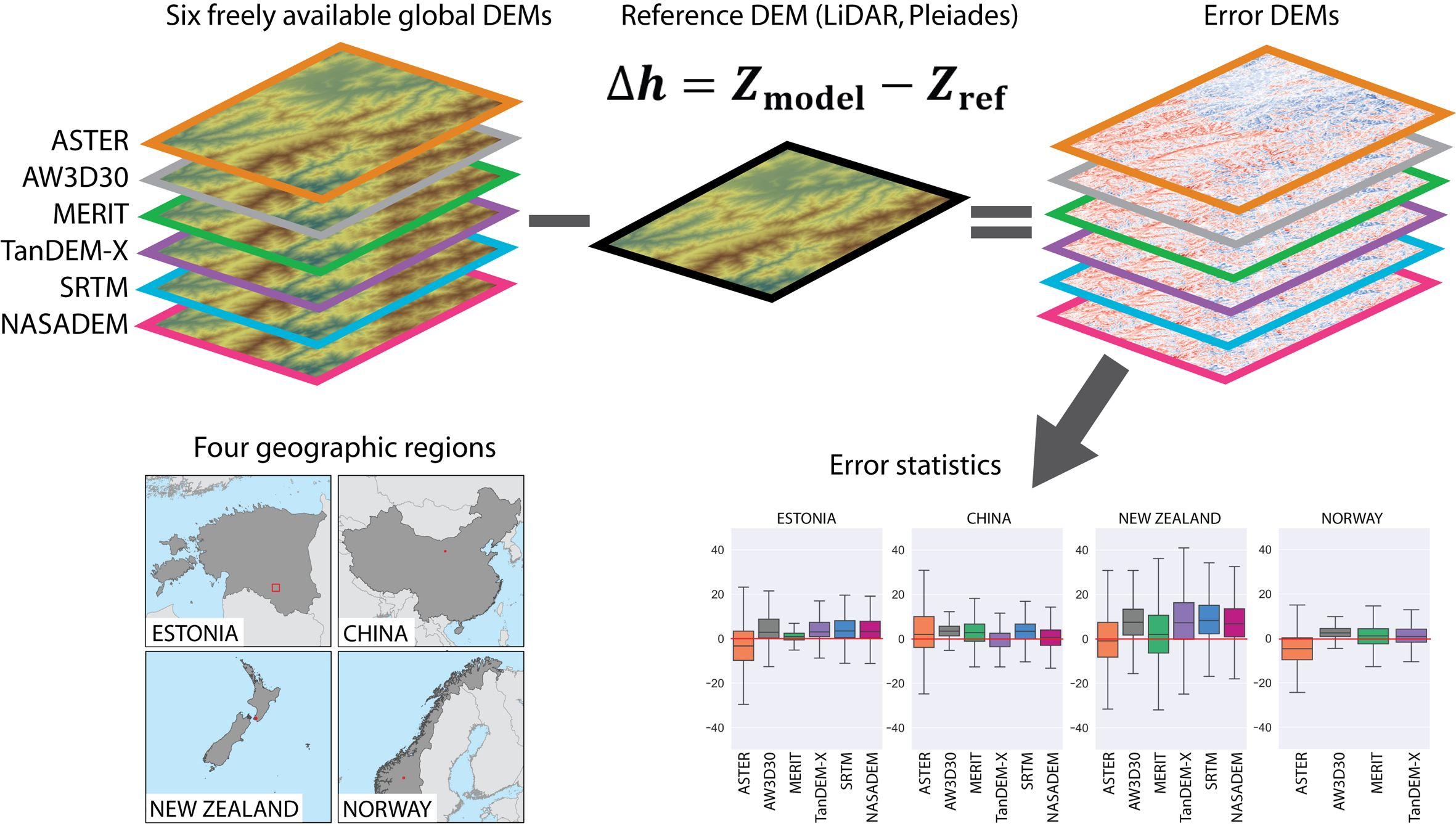
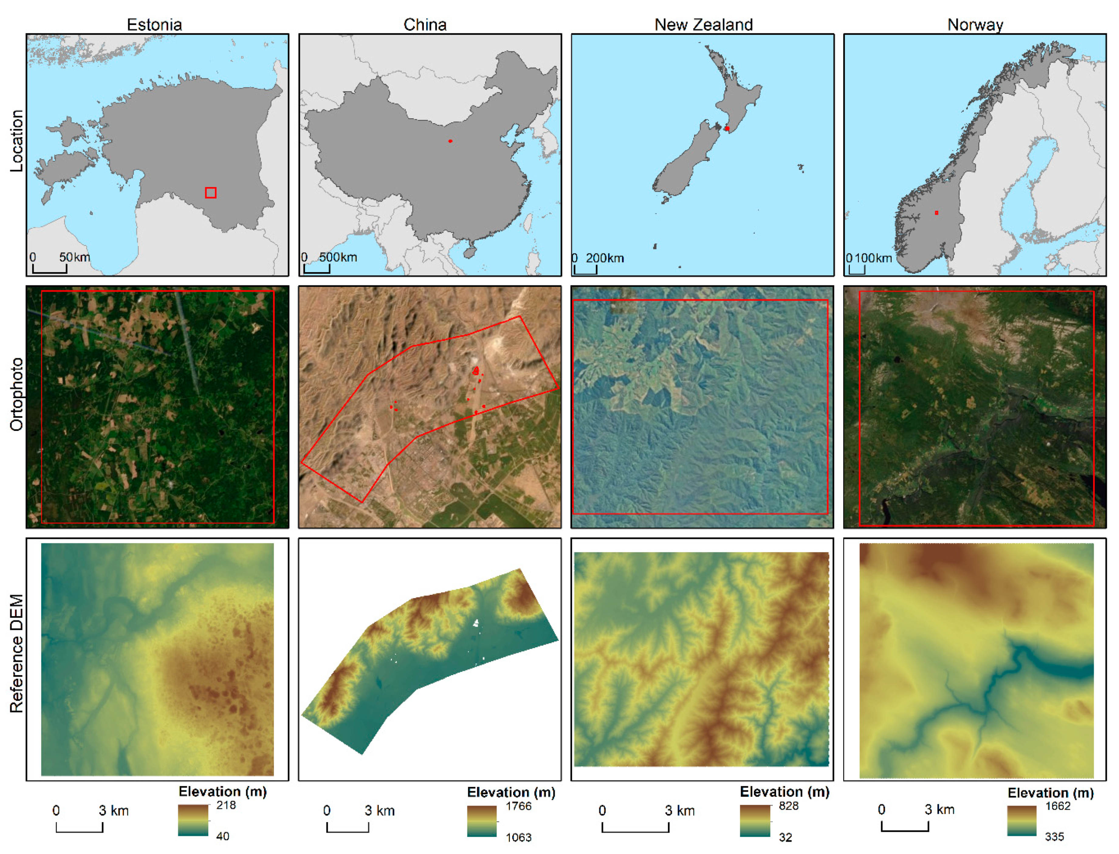
2.1. Study Areas

Four study areas were chosen based on two main criteria: (1) the availability of a LiDAR or other high-precision reference model, and (2) the diversity of the land cover and relief, as these are the main factors known to influence DEM accuracy. We chose study areas where a reference model was freely available and where different topographic conditions (flat, hilly, and mountainous areas) coexisted with various land cover types (Figure 1).

2.1.1. Estonia

The Estonian study area is located in Southern Estonia, and covers 225 km² (Figure 1). About 52% of the study area is covered by closed forest and about 17% is covered by open forest. About 28% of the study area is arable or otherwise cultivated land. The study area includes the small village of Puka, with 565 inhabitants, and several smaller villages. The elevation ranges from 40 to 218 m according to the LiDAR-based reference model (see Section 2.3.1.), and the topography is relatively flat, with some hilly landscapes in the eastern part of the study area (Figure 1).

2.1.2. China

The Chinese study area is located in the Ningxia Hui autonomous region (south of Mongolia). The area is bounded by the Helan Mountains and has tectonic faults that resulted in a diverse relief (Figure 1). In the 103 km² total area, 52% is covered by open land or sparse vegetation, 24% is covered by artificial landscapes (e.g., residential and industrial areas), and 20% by grasslands. The area’s elevation ranges from 1063 to 1766 m (Figure 1).

2.1.3. New Zealand

The study area covers 111 km² and is located in the southern part of North Island of New Zealand in the administrative districts of Lower Hutt City, Upper Hutt City, and South Wairarapa. The dominant land cover types are dense evergreen forests. The other land cover types are grasslands, open forest, shrubs, and arable land. The region’s relief is characterized by mountains and gorges, with elevation ranging from 32 to 828 m.

2.1.4. Norway

The Norwegian study area lies between Jotunheimen and Rondane mountainous areas, and covers 193 km². It is located in the Froni municipality within Innlandet County. The elevation ranges from 335 to 1662 m, but it is relatively flat and does not have many steep slopes. The Vinstra river crosses the study area. Approximately 44% of the study area is covered by forests, 37% by grasslands and 12% by open forest. Water bodies, arable land, and wetlands cover the rest of the area. The SRTM and NASADEM were not available for this study area because it is located above 60°N latitude. Therefore, we only analyzed the ASTER, AW3D30, MERIT, and TanDEM-X DEMs to test the accuracy of these alternative global DEMs for a region where SRTM and NASADEM data are not available.

2.2. The Studied DEMs

Table 1. Summary of the global digital elevation models (DEMs) evaluated in the present study.

Dataset	Horizontal Resolution (m)	Method	Estimated Vertical Accuracy (m)	Data collection Period	Source
ASTER GDEM V3	30	Photogrammetry	17 [33]	2011	[52]
AW3D30	30	Photogrammetry	5 [22]	2006–2011	[53]
MERIT DEM	90	Computational	12 [21]	2000–2017	[54]
TanDEM-X DEM	90	Interferometry synthetic aperture radar	<10 [43]	2011–2015	[55]
SRTM DEM V3	30	Interferometry synthetic aperture radar	9 [48]	2000	[52]
NASADEM	30	Interferometry synthetic aperture radar		2000	[56]

summarizes the characteristics of the DEMs used in the present study.

2.2.1. ASTER

The ASTER Global DEM (GDEM) version 2 (v2) was created photogrammetrically from a compilation of cloud-free ASTER stereopair images [32,33]. The sensor is carried aboard the Terra satellite and the images stereopairs were acquired by nadir- and after-looking angles in the near-infrared band [30,34]. A major advantage of the along-track mode of data acquisition (as compared to cross-track acquisition) is that the images that form the stereopairs are acquired a few seconds apart (rather than days) under uniform environmental and lighting conditions [34]. The ASTER GDEM2 was released in 2011 and showed improvements compared with the first version, such as better georeferencing, inclusion of more scenes acquired between 2008 and 2011, and a smaller correlation kernel, and has higher spatial resolution [33]. However, ASTER GDEM2 is known to have anomalies and artifacts that limit its usefulness [9,35]. Previous studies have found that ASTER GDEM2 performs well over bare areas but is less accurate over areas with a high forest cover [30,36].

2.2.2. AW3D30

The ALOSWorld3D 30 m DEM (AW3D30; version 3.1) was developed based on millions of images acquired by panchromatic optical sensor (PRISM) onboard the Advanced Land Observing Satellite (ALOS) [22]. The stereoscopic images were acquired along-track at nadir, backward and forward views and with 2.5 m of spatial resolution [37]. The first version of AW3D30 was published in 2016 and since then the dataset has been updated to improve the absolute/relative height accuracies with additional calibrations and void filling [22]. The latest version was released in April 2020, which was also used in the current study. Although, the accuracy estimation of the AW3D DEM is available only for the 5 m-resolution commercial version (root-mean-square error (RMSE) of 5 m), studies that have compared different DEM products have shown good accuracy for AW3D30 [38,39].

2.2.3. MERIT

The MERIT DEM was created to provide an error-reduced DEM product. The DEM was developed by combining data acquired from SRTM with data from the ALOS World 3D data with 30 m resolution (AW3D-30m v1), and used error-removal techniques that reduced the bias and other sources of noise [21]. The reported accuracy is ±12 m (90th percentile of the error range) [21]. Studies suggested that the reduced-error DEM performed well [12,28], but that artifacts remain in the DEM product [40].

2.2.4. TanDEM-X DEM

The TanDEM-X DEM was developed based on interferometric synthetic aperture radar (InSAR) images acquired by X-band radar and full polarimetric synthetic aperture radar sensors on two satellites (TerraSAR-X and TanDEM-X) [15,41]. The sensors imaged the Earth’s surface at least twice between 2010 and 2015, and additional images were acquired for areas with complex topography, such as mountain regions. The sensors aboard the satellites orbited the Earth in a twin formation with long track distances ranging from 300 to 500 m, thereby supporting both across-track and along-track interferometry [42]. This approach supported the development of a DEM with high accuracy. The TanDEM-X DEM product with a spatial resolution of 12 m that was released in September 2016 is reported to have a horizontal and vertical absolute accuracy of <10 m, and a relative vertical accuracy of 2 m for slopes ≤11° and 4 m for slopes >11° [43]. As the DEM with 12 m resolution is only available upon approval of a scientific proposal and requires payment of a processing fee, we instead used the completely free TandDEM-X DEM global product (Version 1.0) with 90 m spatial resolution that was released in late 2018 [26]. The quality of the interferometric SAR (InSAR) DEMs are known to be affected by the particular land cover and terrain characteristics of the area under illumination and the specific acquisition geometry used for the data take [15]. SAR acquisitions over complex terrain are often affected by geometric distortions (including foreshortening, layover, and shadow) [15,44], and the X-band signal can partially penetrate vegetation [26] and volume scattering, creating some uncertainty in the height estimation.

2.2.5. SRTM

The SRTM DEM was developed based on the images acquired by two synthetic aperture radars aboard Space Shuttle Endeavour [45,46]. The shuttle flew and mapped continental areas between 60°N and 60°S for 11 days in February 2000. One of the sensors, which used a C-band radar system, was responsible for contiguous mapping coverage, while the other sensor, which used an X-band system, was responsible for generating data along discrete 50-km-wide swaths [45]. The SRTM DEM that we used, with a spatial resolution of 30 m, was developed based on the C-band radar interferometry data and has a reported accuracy of ±16 m [47]. However, the vertical accuracy has also been reported to be <9 m [48] and to be 4.31 m (±14.09 m) in mountain regions [49]. SRTM is known to suffer from voids due to shadow-casting [50]. The accuracy of SRTM is known to suffer from the similar InSAR methodology-related issues as TanDEM-X (see Section 2.2.4). In our study, we used the void-filled SRTM DEM version 3 (SRTMV3) dataset that was released in 2014 [50].

2.2.6. NASADEM

The NASADEM (released in February 2020) was created by reprocessing of the SRTM radar data, and merging it with other DEM datasets, such as ASTER, ICESat and GLAS. The main objective was to eliminate voids and other limitations that were present in the SRTM dataset [23]. The NASADEM is supposed to be the successor of the SRTM DEM dataset [51]. To the best of our knowledge, there are no studies on the accuracy of the NASADEM dataset.

2.3. Reference Models

2.3.1. LiDAR DEMs

We used DEM products derived based on Light Detection and Ranging (LiDAR) data as reference models for the study areas in Estonia, Norway, and New Zealand (China is described in the next section). LiDAR-based DEMs have good accuracy [57], but LiDAR technology cannot penetrate a dense vegetation canopy and the datasets do not cover large areas [32]. For the Estonian study area, we downloaded the DEM from the Estonian Land Board’s Geoportal [58]. The reported vertical accuracy by the Estonian Land Board is 9 to 14 cm. The reference DEM for the Norwegian study area was acquired from Høydedata portal [59] and the reported vertical accuracy is 3 to 12 cm. The New Zealand reference DEM was downloaded from Linz Data Service [60]. The reported vertical accuracy of the New Zealand reference DEM is 10 to 15 cm. All reference DEMs had a 1 m horizontal resolution.

2.3.2. Pleiades-1A DEM

For the Chinese study area, we used the Pleiades-1A DEM because LiDAR data were not available. The Pleiades-1A DEM for the Chinese study area was developed using five image stereopairs acquired by the satellites of the Pleiades mission on 23 April, 17 July, 24 July, and 25 July of 2014 [61]. These images were processed using the photogrammetry module of the ERDAS IMAGINE software. The final DEM was acquired by averaging the point cloud from the image stereopairs within 1 m pixels using continuous-curvature splines in tension and a tension factor of 0.75 [61]. The data were downloaded from OpenTopography portal [62]. No estimated vertical accuracy was provided for the current DEM product, but studies that used similar approaches have reported accuracies from 30 cm [63] to 0.5 m [64].

2.4. Pre-processing

All the datasets had different spatial resolution and different horizontal and vertical reference systems. All global DEMs (except TanDEM-X) originally represented orthometric heights from the EGM96 geoid. However, all of the reference DEMs used different geoids. To make all the study areas comparable, we (1) projected all the datasets to the WGS84 coordinate system; and (2) transferred all DEMs to the EGM96 geoid by subtracting the difference between the local geoid and the EGM96 geoid from the reference DEM values. The elevation values for the TanDEM-X DEM represent ellipsoidal heights, so to convert them to orthometric heights, we subtracted the EMG96 height from the TanDEM-X DEM. All geoid models (except EST-GEOID2017) were downloaded in GeoTIFF format from Agisoft Geoids [65]. EST-GEOID2017 [66] was obtained in ASCII format from the Estonian Land Board. Previous studies have resampled reference models to the global DEM resolution, but this loses information. Therefore, we resampled all global DEMs using the nearest neighbor method and aligned the results spatially to the reference model’s spatial resolution (1 m). Pre-processing was performed in ArcGIS 10.6 [67].

2.5. Accuracy Assessment

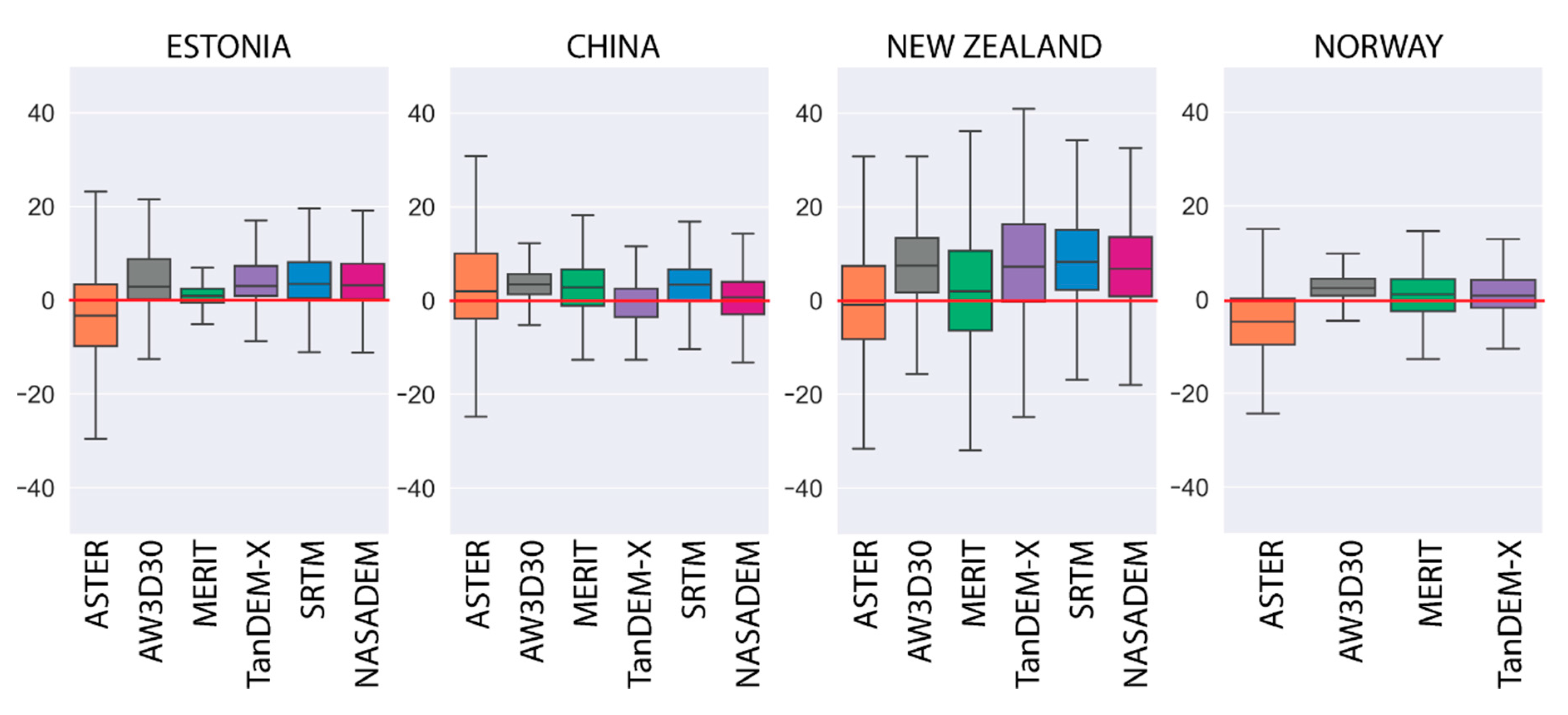
All global elevation models are, strictly speaking, digital surface models (DSMs) [30,32,68]. However, in most applications, they are treated as being equivalent to DEMs [69,70], so for simplicity, we will use the term “DEM” in the rest of this paper. To assess the vertical accuracy of the global DEMs, we created the error rasters on a cell-by-cell basis by subtracting the reference model’s value from the corresponding value in each global DEM:

$$\Delta h=Z_{\mathrm{model}}-Z_{\mathrm{ref}}$$

(1)

where ∆h is the height difference (error) between the global and reference DEM, which was defined as the error term, Z_model is the height in the global DEM, and Z_ref is the height in the reference DEM. We used the map algebra module in ArcGIS 10.6 to generate the error rasters.

To analyze the effect of vegetation on the accuracy of the elevation models, we used the global 100 m-resolution vegetation cover data for the year 2015 from the Copernicus Global Land Cover Layers—Collection 2, which can be freely downloaded from the Copernicus site [71]. The data collection for the global DEMs took place from 2000 to 2017. We initially chose the study areas in relatively remote areas with small land cover change. In addition, to consider the land cover changes, we firstly performed visual check of historical changes based on Google Earth images and CCI long-term global land cover time series (300 m resolution). We identified that the land cover has not changed significantly over the last 10 years. To better align the land cover dataset for the year 2000 (SRTM and NASADEM), we used the Global Forest Change forest cover dataset [72] and added all the forests to the 2015 year land cover to ensure that bare areas are not overestimated in the land cover. Only the Estonian study area had noticeable changes in the forest cover from 2000 to 2015. The NZ and Norwegian study areas remained practically unchanged, and the Chinese study are had no forest. The original 21 land cover classes (Supplementary S1) were generalized and reclassified into 10 classes (

Table 2. Slope, slope aspect, and land cover classes used in the study.

Slope (°)	Slope Class	Azimuth	Aspect	Land Cover Class	Land Cover Type
0–5	1	337.501°–22.5°	N	1	Closed forest
5–10	2	22.501°–67.5°	NE	2	Open forest
10–15	3	67.501°–112.5°	E	3	Shrubs
15–20	4	112.501°–157.5°	SE	4	Herbaceous vegetation
20–25	5	157.501°–202.5°	S	5	Cultivated area
25–30	6	202.501°–247.5°	SW	6	Urban/built up
30–35	7	247.501°–292.5°	W	7	Bare/sparse vegetation
>35	8	292.501°–337.5°	NW	8	Wetland
				9	Snow and ice
				10	Water

). To separate the effect of slope from the effect of land cover, we only used slopes of less than 15° in the land cover analysis.

To analyze the effect of slope and aspect on the accuracy of the DEM, we derived slope and aspect from the reference model DEM (LiDAR or Pleiades-1A). Slope was reclassified into 8 classes (Table 2). Gdulová et al. [24] reported that the relationship between the DEM accuracy and terrain aspect is stronger for greater slopes. Therefore, we extracted slopes steeper than 15° (slope classes 4 to 8 in Table 2) to estimate the effect of aspect on the DEM accuracy. In addition, to eliminate the effect of dense vegetation on the aspect analysis, we only used land cover classes 4, 5, and 7 (classes 9 and 10 were not present on slopes steeper than 15°) in the aspect analysis. We also reclassified aspect from 0° to 360° into 8 cardinal directions (Table 2).

In addition, we calculated roughness for all the study areas because we assumed that higher roughness (variability or irregularity in elevation) results in lower DEM accuracy. We performed correlation analysis which revealed that roughness was highly correlated with slope (0.92 < r2 < 0.98). Therefore, roughness would not have explained the significant amount of additional variation in the errors, and for this reason we did not include it in the further study.

We further analyzed the error rasters together with the land cover, slope, and aspect rasters using Python function libraries. We used the Python rasterio and pandas libraries [73] to transform all the raster data into dataframes in which all spatially aligned error cells were joined with the respective land cover, slope, and aspect class.

For every error raster, we generated a histogram of the errors (Supplementary S2). The histograms let us estimate the error distribution and detect any deviations from a normal distribution. We calculated error metrics across all study areas and also as a function of the land cover, slope, and aspect classes. We used the following error statistics suggested by Höhle and Höhle [74]: the mean error (ME), median error (MedE), root-mean-square error (RMSE), and standard deviation (STD). Several DEMs did not have a normal error distribution (Supplementary S1) and we therefore also calculated more robust accuracy measures suited for non-normal error distributions [74]: the normalized median absolute deviation (NMAD) and the 25% and 75% quantiles. We used the Python NumPy library [75] to calculate the error metrics. In addition, we generated boxplots to visualize the errors. The Python scripts used for these calculations are available in the GitHub repository: https://github.com/LandscapeGeoinformatics/globalDEM_accuracy.

3. Results

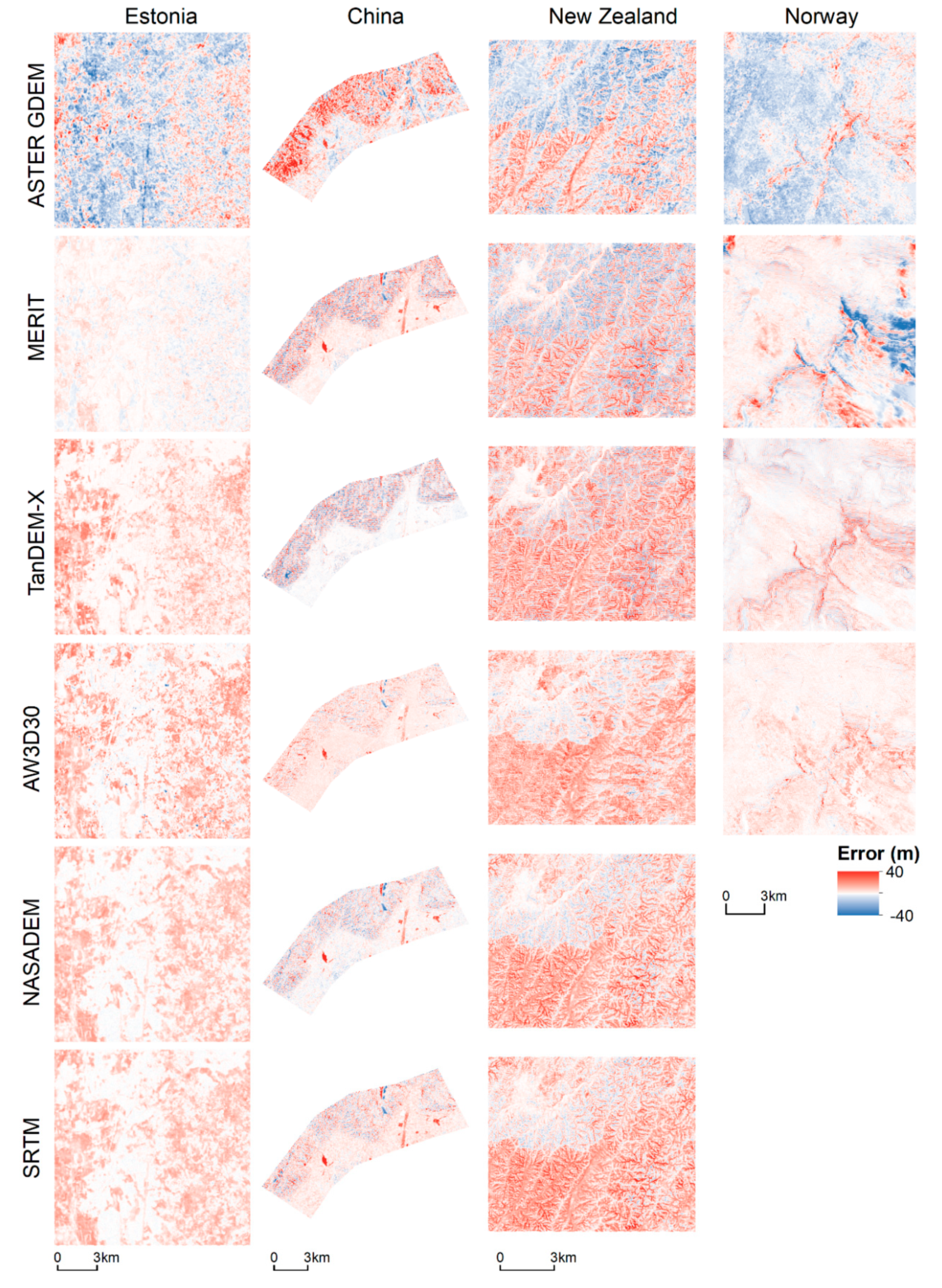
3.1. Overall Vertical Accuracy

For all study areas and elevation models, except for a few cases in ASTER and TanDEM-X, ME and MedE were positive (

Table 3. Error measures for the ASTER, AW3D30, MERIT, TanDEM-X, SRTM, and NASADEM digital elevation models for the four study areas. SRTM and NASADEM data were not available for the Norwegian study area because of its high latitude. Error terms: ME, mean error; STD, standard deviation; 25% and 75%, quantiles; MedE, median error; NMAD, normalized median absolute deviation; RMSE, root-mean-square error.

	Global DEM	No of Pixels	ME	STD	25%	75%	MedE	NMAD	RMSE
Estonia	ASTER	210 787 413	−3.16	9.86	−9.75	3.42	−3.29	7.81	10.36
	AW3D30	210 787 413	4.87	6.25	0.25	8.77	2.89	5.03	7.92
	MERIT	210 787 413	0.87	2.88	−0.57	2.44	0.93	2.11	3.01
	TanDEM-X	210 787 413	4.81	5.31	0.92	7.36	3.06	4.14	7.16
	SRTM	210 787 413	4.57	4.75	0.44	8.11	3.51	4.03	6.59
	NASADEM	210 787 413	4.31	4.72	0.23	7.8	3.21	4	6.39
China	ASTER	99 105 968	3.89	12.95	−3.88	10.02	1.99	9.53	13.52
	AW3D30	99 105 968	3.77	6.11	1.36	5.72	3.5	3.83	7.18
	MERIT	99 105 968	2.76	12.12	−1.07	6.69	2.83	7.57	12.43
	TanDEM-X	99 105 968	−0.51	11.09	−3.55	2.55	-0.05	6.65	11.1
	SRTM	99 105 968	3.27	9.45	−0.13	6.7	3.41	5.73	10
	NASADEM	99 105 968	0.59	8.51	−2.89	4	0.68	5.62	8.53
New Zealand	ASTER	106 101 374	−0.43	11.76	−8.22	7.39	−0.89	9.33	11.77
	AW3D30	106 101 374	7.75	8.38	1.76	13.37	7.48	6.72	11.42
	MERIT	106 101 374	2.38	13.37	−6.39	10.64	2.01	10.41	13.58
	TanDEM-X	106 101 374	8.03	12.74	−0.17	16.27	7.26	10.1	15.05
	SRTM	106 101 374	9	9.47	2.32	15.1	8.27	7.53	13.07
	NASADEM	106 101 374	7.55	9.43	0.95	13.59	6.79	7.49	12.08
Norway	ASTER	192 759 974	−4.36	8.12	−9.57	0.28	−4.7	6.18	9.22
	AW3D30	192 759 974	2.99	3.98	0.86	4.46	2.45	2.69	4.98
	MERIT	192 759 974	0.2	10.49	−2.47	4.35	1.13	6.24	10.49
	TanDEM-X	192 759 974	1.52	6.67	−1.7	4.15	0.87	4.51	6.84

, Figure 2). That is, all the global models generally overestimated the elevation compared to the reference models, which was expected. From the spatial distribution of the errors, it is clear that forested areas had strong positive errors compared to the reference models (Figure 1 and Figure 3). However, in the cases of the Estonian, New Zealand, and Norwegian study areas, ASTER had a negative ME and MedE. The negative errors were spatially occurring in areas with low vegetation cover (Figure 3). The accuracy of AW3D30 was the most stable based on RMSE and STD across the study areas and in most cases also performed the best; however, it slightly overestimated the elevation in all four study areas (Figure 3). Of the six global models, ASTER and in most cases also MERIT performed the worst based on RMSE. Moreover, MERIT showed the largest variation in error values (NMAD between 2.11 and 10.41 m) (Table 3, Figure 2). Of the four study areas, the biggest variation in errors (STD) was observed in New Zealand, where the relief was the most rugged and was combined with tall and dense vegetation (Table 3, Figure 2).

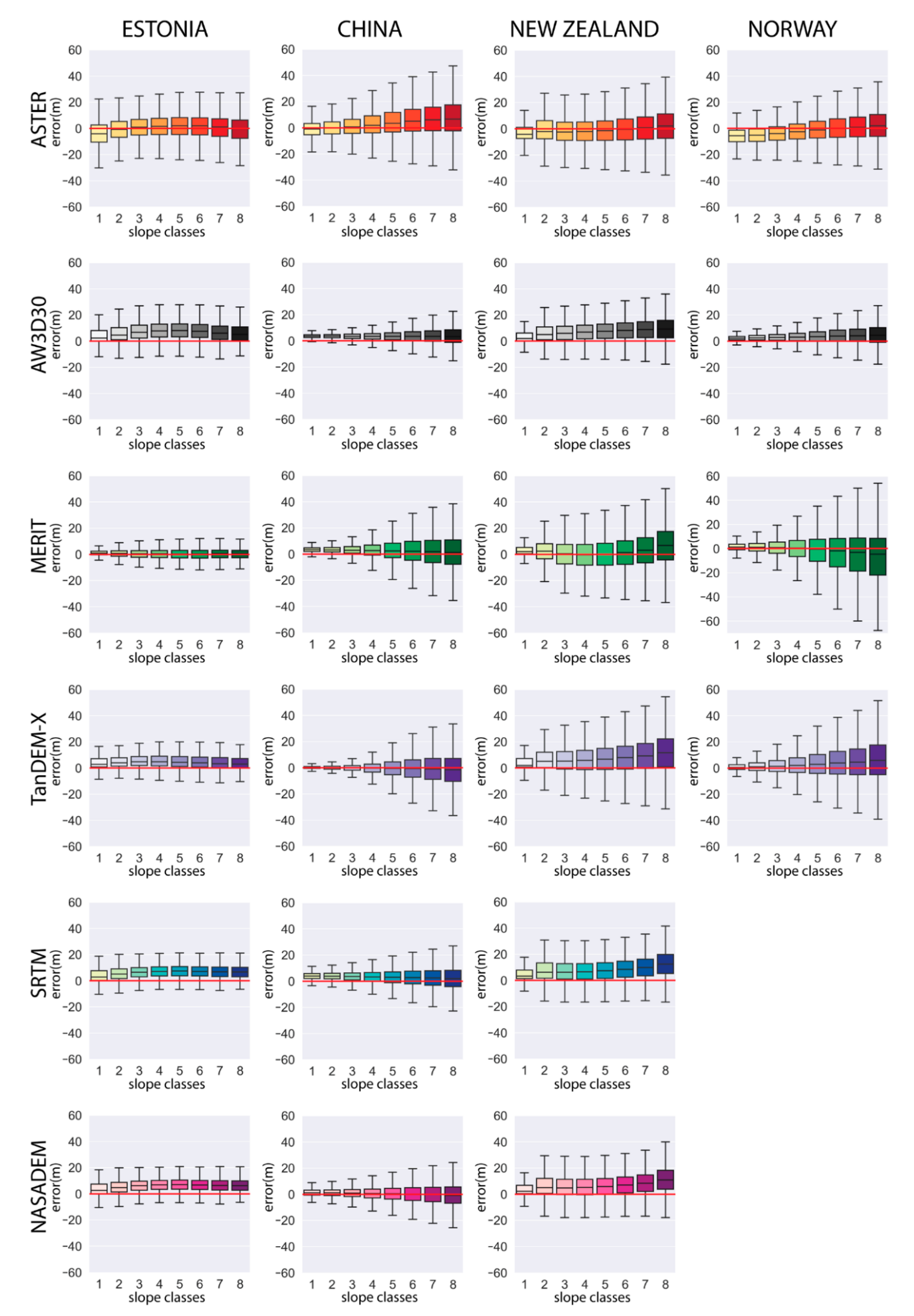
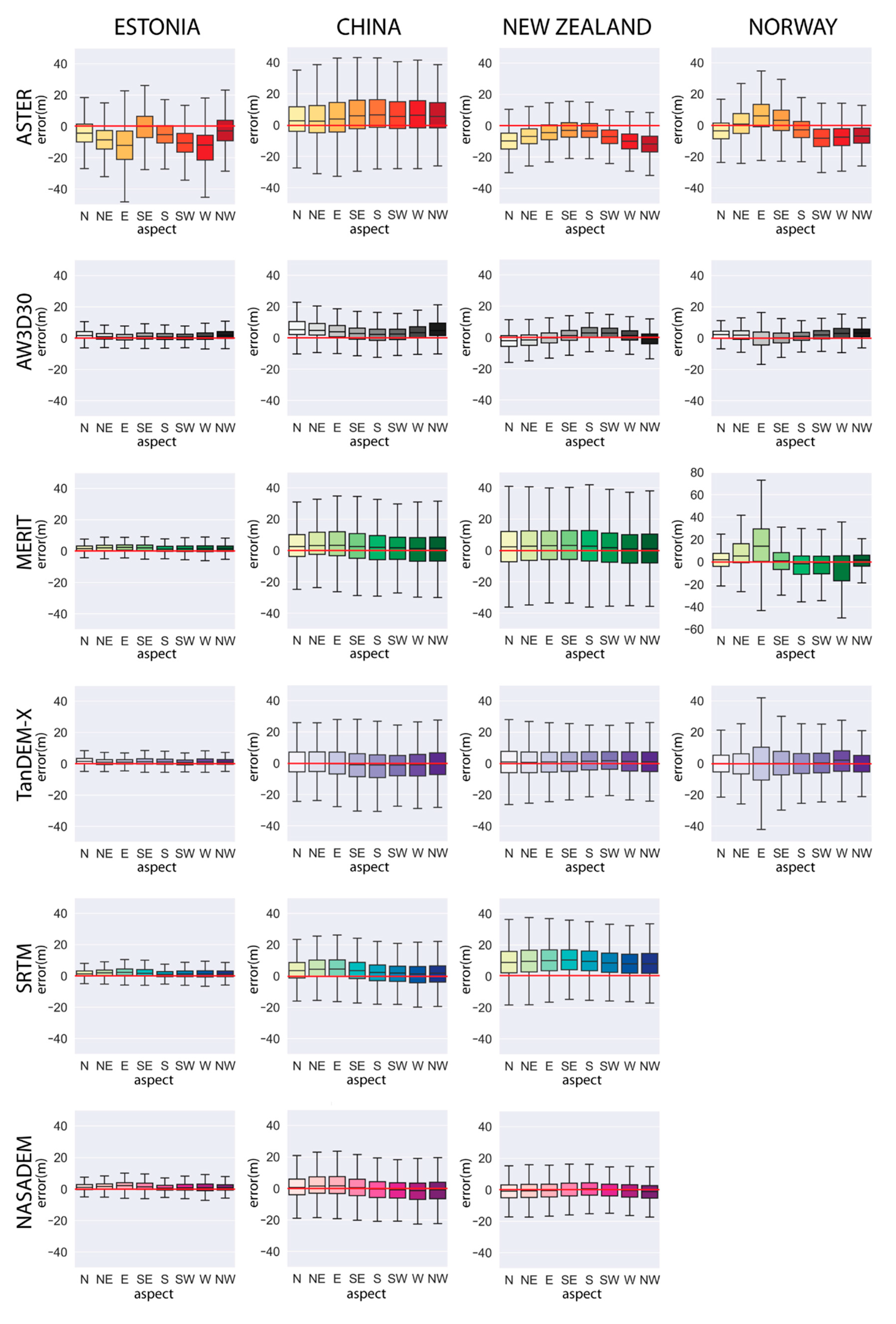
3.2. Effect of Slope and Aspect on Accuracy

There was a clear effect of slope on the vertical accuracy of the DEMs (Figure 4, Supplementary S3a–d) in the Chinese, New Zealand, and Norwegian study areas. The Estonian study area showed no slope effect because most of the study area is flat and 95% of the pixels had a slope less than 10° (Supplementary S4). The effect of slope on accuracy was smallest for the AW3D30, SRTM, and NASADEM. The ASTER, MERIT, and TanDEM-X DEMs exhibited similarly strong effects of slope on their accuracy; with increasing slope, the RMSE and variation of the error (STD) increased (Figure 4, Supplementary S3a–d). MedE showed slightly different behavior among the DEMs. MedE did not have clear increasing nor decreasing pattern for ASTER. For all the other DEMs, MedE in general increased, except for the Chinese study area.

Aspect had a smaller effect on the accuracy of the DEMs than slope (Figure 5). The effect of aspect on accuracy was strongest for the ASTER model; however, there was no clear pattern across study areas (Figure 5). In the Norwegian study area, the E and SE slopes had MedE values of 6.04 and 3.24 m, respectively, whereas the opposing W and NW slopes had MedE values of −7.47 and −6.48 m, respectively. We observed a similar pattern for the New Zealand study area, where E, SE, and S slopes had contrasting MedE values to the opposite W, NW, and N slopes, respectively. However, the Estonian and Chinese study areas did not show similar patterns.

The MERIT model also showed high variation in errors (STD) for all aspects and all study areas except Estonia. However, there was no clear dependency on aspect. The errors in the AW3D30 model had the smallest variation but showed no strong dependency on aspect. In the case of New Zealand and Chinese study areas, AW3D30 even exhibited contrasting patterns. SRTM and NASADEM also showed relatively low variation. For the SRTM and NASADEM, the E and SE slopes had the poorest accuracy (high MedE) among the study areas and NW slopes had the highest accuracy (low MedE) (Figure 5, Supplementary S5a–c). TanDEM-X did not show any dependency on aspect.

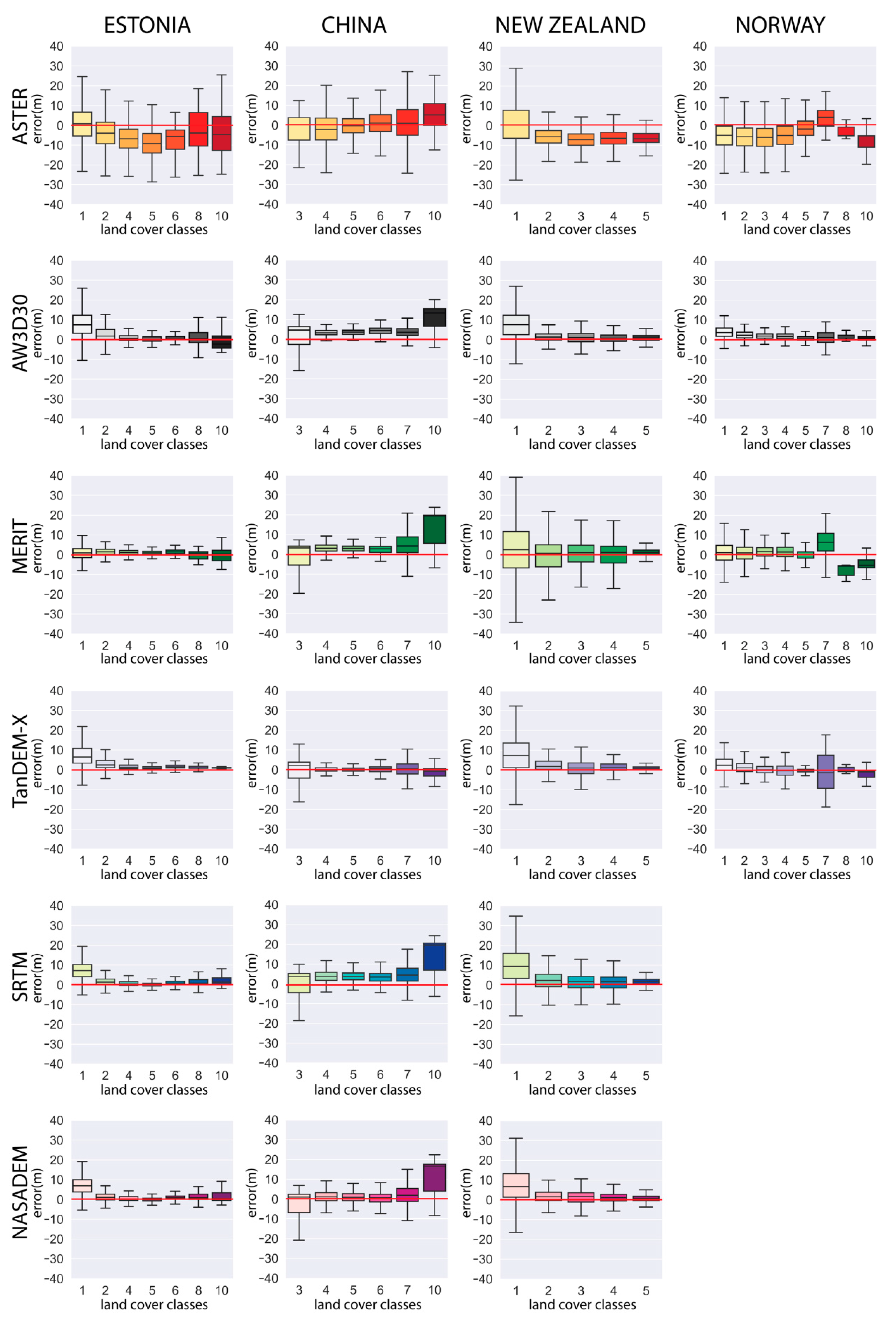
3.3. Effect of Land Cover on Accuracy

We found that all DEMs had systematically higher elevations than the actual land surface in forested areas in land cover classes 1 and 2 (Figure 6, Supplementary S6a–c). MedE was consistently positive for all the DEMs, except for the ASTER model in the Estonian study area, and RMSE ranged from 3.54 to 13.66 m for the closed forest and 2.82 to 10.5 m for the open forest across study areas. We observed the highest errors and variation (STD) for forested areas in the New Zealand study area. From all six global models, the AW3D30 was the most accurate over the forested areas across all study areas.

The DEMs were generally more accurate for the herbaceous and cultivated areas (land cover classes 4 and 5) than for the forested areas (Figure 6, Supplementary S6a–d). In most cases, the global models slightly overestimated (positive MedE) the elevation over the herbaceous and cultivated areas. The RMSE was less than 5 m in most cases, except for the ASTER DEM, for which the RMSE was mostly greater than 5 m and often greater than 10 m. The ASTER DEM also often underestimated the elevation for herbaceous and cultivated areas. There was no single best performing DEM over the herbaceous and cultivated areas. Some DEMs that showed high accuracy in some study areas did not have good accuracy in some others (e.g., MERIT). However, AW3D30 showed most consistent and in most cases also the best accuracy across all study areas.

The magnitude of the error for the urban and built-up areas (land cover class 6) was similar to the values for herbaceous and cultivated areas. For urban and built-up areas, the MedE values were −5.56 to 4.39 m, which was similar to the values for herbaceous and cultivated areas. All DEMs, except for TanDEM-X, strongly overestimated the elevation over water (land cover class 10) in the Chinese study area (Supplementary S6b).

4. Discussion

4.1. Overall Accuracy

AW3D30 provided the most robust and accurate DEM for all regions, which aligns with previous studies that found that the vertical RMSE was below 5m in flat areas [16,76] and rises up to 12 or to 14 m in areas with more complex relief [76].

The next-best DEMs were SRTM and NASADEM. For the SRTM, previous studies reported a vertical accuracy (RMSE) of 5 m [30] using GPS ground-control points, and 14.9 m (RMSE) by using LiDAR as the reference model [32]. Our results agree with these previous studies, as we found the overall RMSE to be 6.59, 10.00, and 13.07 m in the Estonian, Chinese, and New Zealand study areas, respectively. The recently released NASADEM, which is supposed to be the successor for the SRTM, showed only slightly better accuracy with the overall RMSE found to be 6.39, 8.53, and 12.08 m in the Estonian, Chinese, and New Zealand study areas, respectively.

For the MERIT model, we found an overall accuracy (RMSE) of 3.01, 12.43, 13.58, and 10.49 m for the Estonian, Chinese, New Zealand, and Norwegian study areas, respectively. For the TanDEM-X DEM, overall RMSE was 7.16, 11.10, 15.05, and 6.84 m for the Estonian, Chinese, New Zealand, and Norwegian study areas, respectively. These fall within the expected accuracy range in previous research: 12 m for MERIT [21] and 10 m for TanDEM-X [15]. However, some studies have identified better accuracies. For example, Hawker et al. [26] estimated the RMSE to be 2.32 and 3.10 m for MERIT and TanDEM-X, respectively. Our error estimates are probably higher because of the more complex terrain in our study areas; however, in the flat Estonian study area, our results are similar to these previous results. MERIT and TanDEM-X are more sensitive than SRTM to relief, mainly due to the lower spatial resolution; this leads to intra-pixel variation, which is exacerbated on steep slopes.

ASTER performed the worst of the models in all study areas (RMSE 9.22 to 13.52 m). It also had the highest uncertainty (high STD) across study areas for a range of topographic conditions and land cover types. Several studies have found similar accuracy for ASTER [32,33]. The ASTER DEM also includes artifacts that are likely due to cloud cover, mismatches between different scenes, and processing techniques which is its major shortcoming [9,30].

4.2. Effect of Slope and Aspect on Accuracy

The slope had the strongest effect on the accuracy of the global DEMs. For all six global DEMs, the uncertainty increased with the increasing slope. The ASTER, MERIT and TanDEM-X were the most affected by slope. The RMSE rose from between 8.25 and 10.62 m on slopes <5° to between 10.25 and 23.35 m on slopes >35° for ASTER; from between 2.83 and 7.25 m on slopes <5° to between 4.67 and 26.85 m on slopes >35° for MERIT; from between 3.27 and 8.06 m on slopes <5° to between 8.12 and 19.23 m on slopes >35° for TanDEM-X (Supplementary S3a–d). This agrees well with previous studies [24,26,77,78]. We resampled all the global DEMs to agree with the reference model resolution (1 m), which results in higher intra-pixel variation on steeper slopes. This effect can be clearly seen in the error map for the New Zealand study area (Figure 3), which had the most complex topography and where intra-pixel variation is clearly visible for the lower-resolution MERIT and TanDEM-X DEMs. The accuracy of the AW3D30, SRTM and NASADEM models was the least affected by slope and their variation in error did not increase so much as compared to ASTER, MERIT and TanDEM-X.

ASTER showed the biggest variation in errors (STD) and AW3D30 showed the smallest variation due to aspect, but no clear dependency on aspect. The high variation of the errors and the overall random response to aspect is likely caused by artifacts in the ASTER model. The visual inspection of numerous artifacts in the ASTER model (Figure 3) and the high variation in errors across the study areas demonstrated the model’s lower quality, which was previously described by Purinton and Bookhagen [10].

For the SRTM and NASADEM, we observed a small systematic dependency on aspect in which opposite directions (e.g., NW and SE) had contrasting accuracy. This was observed previously by Szabó et al. [79] and Gorokhovich and Voustianiouk [80]. They related this dependency to the orbit of Space Shuttle Endeavour, which was perpendicular to the NE–SW line. The quality of synthetic aperture radar (SAR) images depends upon the view direction. In the view direction, inclined terrain causes foreshortening or even layover (i.e., when the beam encounters the top of an object before it encounters the base) [81]. Previous studies have identified similar issues for the TanDEM-X DEM. Gdulová et al. [24] observed the poorest accuracy for east-facing slopes; this resulted from the presence of areas with data acquisition only from an ascending orbit. However, our study did not identify this pattern. East-facing slopes only exhibited higher errors in Norwegian study area, and this was also observed for the MERIT and ASTER DEMs. The highest errors occurred on the steep banks of the Vinstra river valley, which is mostly oriented from NE to SW (Figure 3).

4.3. Effect of Land Cover on the Accuracy

In general, the magnitude of the error for the different land cover types differed more among study areas than among the different DEMs. This indicates that the land cover affects a DEM’s accuracy in ways that are location-specific. Even for a given land cover type, the vegetation characteristics (density, height) vary enough among biomes that the variation causes significant variation in the errors of the DEMs. For SAR-based DEMs (TanDEM-X, SRTM, NASADEM), volume scattering causes uncertainty [79]. In the case of volume scattering in a forest, leaves reflect radar signals which then hit more leaves and branches, and multiple scattering occurs until the signals exit the vegetation. A percentage of the incoming radar is therefore volumetrically scattered back to the SAR sensor, giving the vegetation a brighter signature. However, if the forest height is homogeneous, then the forest surface will still mimic the underlying topography. Forested areas caused a positive bias (i.e., overestimation of the true elevation) in all global DEMs and all study areas. Elevation estimation in forested areas performed most poorly in the New Zealand study area, which is mostly covered by indigenous forests: Nothofagus spp. (beech), broadleaved angiosperm trees, Agathis australis (kauri), and other conifers (predominantly podocarps) form a tall and dense canopy [82]. This canopy may explain the larger positive bias in the New Zealand study area than in the other study areas.

Urban areas produced elevation estimates that were 2 to 5 m higher than the reference model, which was less than the error magnitude we expected. For example, González-Moradas and Viveen [30] found that buildings severely affected the performance of ASTER. As only the Estonian and Chinese study areas (Supplementary S4) had urban areas in flat areas and most of the urban areas were dominated by low buildings or roads, this explains the generally good performance of the global models in the urban parts of these study areas.

The ASTER, MERIT, and SRTM DEMs overestimated the elevation over bodies of water. For the SRTM and MERIT DEMs, this is likely caused by how SAR interferometry functions, since low coherence or low backscatter increases the noise over water [15]. Although SRTM v3 voids have been filled by using the ASTER DEM to improve the SRTM DEM’s water mask [50], ASTER strongly overestimated elevations above bodies of water in the Chinese study area (Figure 3), because small bodies of water were not depicted in the ASTER water mask [83]. Therefore, the SRTM correction was not successful in the Chinese study area. Interestingly, TanDEM-X is also based on interferometry, but did not exhibit large errors over the bodies of water, probably because of having a higher quality water mask.

In principle, all the global DEMs we analyzed can be considered DSMs. This also explains their tendency to overestimate elevation over vegetated areas because the surface that reflects the signal (e.g., a tree canopy rather than the forest floor) exists at some height above the true ground level. However, in case of SAR-based elevation models, there exist some exceptions for areas where the SAR signal penetrates the surface by some meters—e.g., in cases of ice, snow or vegetation [84,85]. It has been shown that for ice and snow, up to 7 m underestimation can take place [86]. In case of forested areas, the overestimation will still happen because the forest height usually exceeds the penetration. However, for MERIT, an approximate vegetation correction has been applied for vegetation but with no comparable correction for buildings [70]. As a result, MERIT exhibited slightly better performance over densely forested areas than the other models.

4.4. Effect of Spatial Resolution

The ASTER, AW3D30, SRTM, and NASADEM had 30 m spatial resolution, but MERIT and TanDEM-X had only 90 m spatial resolution. Despite its higher resolution, ASTER performed worse than MERIT and TanDEM-X. However, in rugged terrain such as the New Zealand study area, we observed high variation of errors and a higher RMSE that can probably be explained by the low spatial resolution, which causes high error variation due to the DEM’s inability to capture variation within the large pixels. Elevation can change significantly on steep slopes within a horizontal distance of 90 m. The elevation estimates around the center of the pixel are likely to be correct, but upslope values are likely to be underestimated and downslope values to be overestimated. This was most apparent for the New Zealand study area (Figure 3). However, Hawker et al. [26] demonstrated that on floodplains, the 90 m TanDEM-X DEM performed better than the 30 m SRTM DEM and similarly to the 90 m MERIT DEM. For geomorphological mapping, high-resolution (12 m) TanDEM-X has been found to yield a detailed and widely consistent landscape representation, and most major landforms can also be easily allocated in the SRTM; however, ASTER does not allow identification of microscale landforms because of the high number of artifacts [87]. González-Moradas and Viveen [30] found that the 12 m resolution TanDEM-X DEM displayed the most accurate elevation values but that the 30 m SRTM DEM also performed well in terms of hydrological applications compared to other 30 m DEMs.

4.5. Limitations of Our Study

One of the limitations of our study was the land cover dataset. To ensure the consistency across all study areas, we used the Copernicus Global Land Cover dataset, with 100 m resolution, which is lower than the resolution of the analyzed DEMs. The coarser spatial resolution might have created errors in land cover classification at the edges of land cover types, where closed forest might have been classified as open forest and vice versa, causing incorrect attribution of errors to some of the land cover types. Another issue is the temporal change of land cover. The global DEM data were collected from 2000 to 2017 and land cover can change significantly. However, our study areas were in remote regions with minimal land cover change and for the year 2000, we used the high-resolution Global Forest Canopy Height dataset [88] to update the 2015 year land cover dataset to ensure that forested areas are the most accurate. In addition, seasonal differences (leaves on–off, dry–wet) affect the collection of the SAR based elevation data because these factors may either increase or decrease the backscatter [89]. Dry conditions usually increase the penetration. The SRTM data are collected in February when it is winter in the northern hemisphere and most of the trees have no leaves, which should increase the penetration. However, evergreen forests still have leaves all year round and are harder to penetrate and the timing of the wet and dry seasons vary across the world.

Several studies have attempted to develop methods to improve the accuracy of global DEMs by data fusion. For example, Yue et al. [90] combined SRTM-1, ASTER GDEM v2, and ICESat laser altimetry data by using ASTER GDEM v2 data as the elevation source for the SRTM void filling and the ICESat GLAS data to increase the accuracy of the ASTER data within the void regions by applying an artificial neural network model. Su et al. [91] developed a regression model based on tree height, canopy cover, and terrain slope to correct the SRTM DEM data in vegetated mountain areas. However, they noted that the limited availability of small-footprint LiDAR data may make it difficult to perform large-scale correction for the SRTM DEM. The recently released NASADEM, which is the updated version of SRTM, was improved by using the new unwrapping strategy [92] to reduce voids, and applying vertical and tilt adjustments based on ground control points derived from the ICESat laser altimeter to improve the elevation estimation over forested areas and snow/ice [23]. The NASADEM development team has also evaluated the extent to which ASTER GDEM3 with cloud removal can be used outside the SRTM latitude range to extend the NASADEM to polar areas [23]. However, based on our study and previous research, AW3D30 would be much more promising. Many studies covered large and geographically diverse regions, and the main reason for using freely available global DEMs is that no high-quality local DEM is available. Moreover, it is unlikely that these regions have high-quality field data over large regions that can be used to improve the global DEM. However, some new global-level datasets, such as Global Forest Change forest height dataset [88], would be promising to apply vegetation correction to NASADEM. Our results show that currently, the most accurate freely available DEM is AW3D30. However, higher-quality commercial products, for example, global TanDEM-X 12m-resolution DEM, have shown higher elevation accuracy [15,31].

5. Conclusions

The accuracy of the global DEMs depended greatly on the unique characteristics of each region. The ASTER model was the least accurate and had the highest uncertainty across all study areas, topographic conditions, and land cover types. AW3D30 showed the smallest uncertainty and highest accuracy across all study areas. However, NASADEM also showed very similar accuracy but it does not cover the northernmost latitudes. MERIT and TanDEM-X performed well despite their lower spatial resolution, and as they also cover higher latitudes. We found slope to be the most important factor affecting DEM accuracy. The smallest bias in the elevation values was detected on flat areas (slope <5°), and the bias increased with increasing slope, thereby increasing variation of the errors. Aspect did not systematically affect DEM performance, which agrees with previous studies. Densely forested areas caused height overestimation by all DEMs. However, MERIT was slightly less affected by the forested areas, mainly due to the vegetation removal procedure. Other DEMs could benefit from similar vegetation correction by employing the new Global Forest Canopy Height dataset.

References

1. Papaioannou, G.; Loukas, A.; Vasiliades, L.; Aronica, G.T. Flood inundation mapping sensitivity to riverine spatial resolution and modelling approach. Nat. Hazards 2016. [Google Scholar] [CrossRef]
2. Bajat, B.; Blagojević, D.; Kilibarda, M.; Luković, J.; Tošić, I. Spatial analysis of the temperature trends in Serbia during the period 1961–2010. Theor. Appl. Clim. 2015, 121, 289–301. [Google Scholar] [CrossRef]
3. Saint-Laurent, D.; Paradis, R.; Drouin, A.; Gervais-Beaulac, V. Impacts of floods on organic carbon concentrations in alluvial soils along hydrological gradients using a digital elevation model (DEM). Water 2016, 8, 208. [Google Scholar] [CrossRef] [Green Version]
4. Balzter, H.; Cole, B.; Thiel, C.; Schmullius, C. Mapping CORINE land cover from Sentinel-1A SAR and SRTM digital elevation model data using random forests. Remote Sens. 2015, 7, 14876–14898. [Google Scholar] [CrossRef] [Green Version]
5. Rahmati, O.; Yousefi, S.; Kalantari, Z.; Uuemaa, E.; Teimurian, T.; Keesstra, S.; Pham, T.D.; Bui, D.T. Multi-hazard exposure mapping using machine learning techniques: A case study from Iran. Remote Sens. 2019, 11, 1943. [Google Scholar] [CrossRef] [Green Version]
6. Scown, M.W.; Thoms, M.C.; De Jager, N.R. Floodplain complexity and surface metrics: Influences of scale and geomorphology. Geomorphology 2015, 245, 102–116. [Google Scholar] [CrossRef]
7. Fenta, A.A.; Kifle, A.; Gebreyohannes, T.; Hailu, G. Spatial analysis of groundwater potential using remote sensing and GIS-based multi-criteria evaluation in Raya Valley, northern Ethiopia. Hydrogeol. J. 2014, 23, 195–206. [Google Scholar] [CrossRef]
8. Bonilla-Sierra, V.; Scholtès, L.; Donzé, F.V.; Elmouttie, M.K. Rock slope stability analysis using photogrammetric data and DFN–DEM modelling. Acta Geotech. 2015, 10, 497–511. [Google Scholar] [CrossRef]
9. Lakshmi, S.E.; Yarrakula, K. Review and critical analysis on digital elevation models. Geofizika 2019, 35, 129–157. [Google Scholar] [CrossRef]
10. Purinton, B.; Bookhagen, B. Validation of digital elevation models (DEMs) and comparison of geomorphic metrics on the southern Central Andean Plateau. Earth Surf. Dyn. 2017. [Google Scholar] [CrossRef] [Green Version]
11. Jarihani, A.A.; Callow, J.N.; McVicar, T.R.; Van Niel, T.G.; Larsen, J.R. Satellite-derived Digital Elevation Model (DEM) selection, preparation and correction for hydrodynamic modelling in large, low-gradient and data-sparse catchments. J. Hydrol. 2015, 524, 489–506. [Google Scholar] [CrossRef]
12. Hawker, L.; Bates, P.; Neal, J.; Rougier, J. Perspectives on digital elevation model (DEM) simulation for flood modeling in the absence of a high-accuracy open access global DEM. Front. Earth Sci. 2018, 6, 1–9. [Google Scholar] [CrossRef] [Green Version]
13. Smith, B.; Sandwell, D. Accuracy and resolution of shuttle radar topography mission data. Geophys. Res. Lett. 2003, 30, 3–6. [Google Scholar] [CrossRef] [Green Version]
14. Eineder, M. Problems and solutions for Insar digital elevation model generation of mountainous terrain. Aerospace 2000, 2003, 1–5. [Google Scholar]
15. Rizzoli, P.; Martone, M.; Gonzalez, C.; Wecklich, C.; Borla Tridon, D.; Bräutigam, B.; Bachmann, M.; Schulze, D.; Fritz, T.; Huber, M.; et al. Generation and performance assessment of the global TanDEM-X digital elevation model. ISPRS J. Photogramm. Remote Sens. 2017, 132, 119–139. [Google Scholar] [CrossRef] [Green Version]
16. Hu, Z.; Peng, J.; Hou, Y.; Shan, J. Evaluation of recently released open global digital elevation models of Hubei, China. Remote Sens. 2017, 9, 262. [Google Scholar] [CrossRef] [Green Version]
17. Ariza-Villaverde, A.B.; Jiménez-Hornero, F.J.; Gutiérrez de Ravé, E. Influence of DEM resolution on drainage network extraction: A multifractal analysis. Geomorphology 2015, 241, 243–254. [Google Scholar] [CrossRef]
18. Dong, Y.; Chang, H.C.; Chen, W.; Zhang, K.; Feng, R. Accuracy assessment of GDEM, SRTM, and DLR-SRTM in Northeastern China. Geocarto Int. 2015. [Google Scholar] [CrossRef]
19. Walczak, Z.; Sojka, M.; Wrózyński, R.; Laks, I. Estimation of polder retention capacity based on ASTER, SRTM and LIDAR DEMs: The case of Majdany Polder (West Poland). Water 2016, 8, 230. [Google Scholar] [CrossRef]
20. Varga, M.; Bašić, T. Accuracy validation and comparison of global digital elevation models over Croatia. Int. J. Remote Sens. 2015. [Google Scholar] [CrossRef]
21. Yamazaki, D.; Ikeshima, D.; Tawatari, R.; Yamaguchi, T.; O’Loughlin, F.; Neal, J.C.; Sampson, C.C.; Kanae, S.; Bates, P.D. A high-accuracy map of global terrain elevations. Geophys. Res. Lett. 2017, 44, 5844–5853. [Google Scholar] [CrossRef] [Green Version]
22. Takaku, J.; Tadono, T.; Doutsu, M.; Ohgushi, F.; Kai, H. Updates of “AW3D30” ALOS global digital surface model with other open access datasets. ISPRS Int. Arch. Photogramm. Remote Sens. Spat. Inf. Sci. 2020. [Google Scholar] [CrossRef]
23. Crippen, R.; Buckley, S.; Agram, P.; Belz, E.; Gurrola, E.; Hensley, S.; Kobrick, M.; Lavalle, M.; Martin, J.; Neumann, M.; et al. Nasadem global elevation model: Methods and progress. In International Archives of the Photogrammetry, Remote Sensing and Spatial Information Sciences—ISPRS Archives; XXIII ISPRS Congress: Prague, Czech Republic, 2016; Volume XLI-B4. [Google Scholar]
24. Gdulová, K.; Marešová, J.; Moudrý, V. Accuracy assessment of the global TanDEM-X digital elevation model in a mountain environment. Remote Sens. Environ. 2020, 241, 111724. [Google Scholar] [CrossRef]
25. Bhardwaj, A. Assessment of Vertical Accuracy for TanDEM-X 90 m DEMs in Plain, Moderate, and Rugged Terrain. Proceedings 2019, 24, 6208. [Google Scholar] [CrossRef] [Green Version]
26. Hawker, L.; Neal, J.; Bates, P. Accuracy assessment of the TanDEM-X 90 Digital Elevation Model for selected floodplain sites. Remote Sens. Environ. 2019, 232. [Google Scholar] [CrossRef]
27. Moudrý, V.; Lecours, V.; Gdulová, K.; Gábor, L.; Moudrá, L.; Kropáček, J.; Wild, J. On the use of global DEMs in ecological modelling and the accuracy of new bare-earth DEMs. Ecol. Modell. 2018, 383, 3–9. [Google Scholar] [CrossRef]
28. Liu, K.; Song, C.; Ke, L.; Jiang, L.; Pan, Y.; Ma, R. Global open-access DEM performances in Earth’s most rugged region High Mountain Asia: A multi-level assessment. Geomorphology 2019, 338, 16–26. [Google Scholar] [CrossRef]
29. Schumann, G.J.-P.; Bates, P.D. The The need for a high-accuracy, open-access global DEM. Front. Earth Sci. 2018, 6, 1–5. [Google Scholar] [CrossRef]
30. del Rosario González-Moradas, M.; Viveen, W. Evaluation of ASTER GDEM2, SRTMv3.0, ALOS AW3D30 and TanDEM-X DEMs for the Peruvian Andes against highly accurate GNSS ground control points and geomorphological-hydrological metrics. Remote Sens. Environ. 2020. [Google Scholar] [CrossRef]
31. Zhang, K.; Gann, D.; Ross, M.; Robertson, Q.; Sarmiento, J.; Santana, S.; Rhome, J.; Fritz, C. Accuracy assessment of ASTER, SRTM, ALOS, and TDX DEMs for Hispaniola and implications for mapping vulnerability to coastal flooding. Remote Sens. Environ. 2019, 225, 290–306. [Google Scholar] [CrossRef]
32. Dewitt, J.D.; Warner, T.A.; Conley, J.F. Comparison of DEMS derived from USGS DLG, SRTM, a statewide photogrammetry program, ASTER GDEM and LiDAR: Implications for change detection. GISci. Remote Sens. 2015, 52, 179–197. [Google Scholar] [CrossRef]
33. Tachikawa, T.; Kaku, M.; Iwasaki, A.; Gesch, D.; Oimoen, M.; Zhang, Z.; Danielson, J.; Krieger, T.; Curtis, B.; Haase, J.; et al. ASTER global digital elevation model version 2—Summary of validation results. Arch. Cent. Jt. Japan US ASTER Sci. Team 2011, 2, 1–25. [Google Scholar]
34. Hirano, A.; Welch, R.; Lang, H. Mapping from ASTER stereo image data: DEM validation and accuracy assessment. ISPRS J. Photogramm. Remote Sens. 2003, 57, 356–370. [Google Scholar] [CrossRef]
35. Florinsky, I.V.; Skrypitsyna, T.N.; Luschikova, O.S. Comparative accuracy of the AW3D30 DSM, ASTER GDEM, and SRTM1 DEM: A case study on the Zaoksky testing ground, central European Russia. Remote Sens. Lett. 2018, 9, 706–714. [Google Scholar] [CrossRef]
36. Gesch, D.B.; Oimoen, M.J.; Evans, G.A. Accuracy Assessment of the U.S. Geological Survey National Elevation Dataset, and Comparison with Other Large-Area Elevation Datasets-SRTM and ASTER. Open-File Rep. 2014. [Google Scholar] [CrossRef]
37. Takaku, J.; Tadono, T.; Tsutsui, K. Generation of high resolution global DSM from ALOS PRISM. ISPRS Int. Arch. Photogramm. Remote. Sens. Spat. Inf. Sci. 2014, 40, 243–248. [Google Scholar] [CrossRef] [Green Version]
38. Courty, L.G.; Soriano-Monzalvo, J.C.; Pedrozo-Acuña, A. Evaluation of open-access global digital elevation models (AW3D30, SRTM, and ASTER) for flood modelling purposes. J. Flood Risk Manag. 2019, 12, 1–14. [Google Scholar] [CrossRef] [Green Version]
39. Jain, A.O.; Thaker, T.; Chaurasia, A.; Patel, P.; Singh, A.K. Vertical accuracy evaluation of SRTM-GL1, GDEM-V2, AW3D30 and CartoDEM-V3.1 of 30-m resolution with dual frequency GNSS for lower Tapi Basin India. Geocarto Int. 2018, 33, 1237–1256. [Google Scholar] [CrossRef]
40. Hirt, C. Artefact detection in global digital elevation models (DEMs): The Maximum Slope Approach and its application for complete screening of the SRTM v4.1 and MERIT DEMs. Remote Sens. Environ. 2018, 207, 27–41. [Google Scholar] [CrossRef] [Green Version]
41. Gruber, A.; Wessel, B.; Martone, M.; Roth, A. The TanDEM-X DEM mosaicking: Fusion of multiple acquisitions using InSAR quality parameters. IEEE J. Sel. Top. Appl. Earth Obs. Remote Sens. 2016, 9, 1047–1057. [Google Scholar] [CrossRef]
42. Zink, M.; Bachmann, M.; Bräutigam, B.; Fritz, T.; Hajnsek, I.; Krieger, G.; Moreira, A.; Wessel, B. TanDEM-X: The new global DEM takes shape. IEEE Geosci. Remote Sens. Mag. 2014, 2, 8–23. [Google Scholar] [CrossRef]
43. Wessel, B. TanDEM-X Ground Segment DEM Products Specification Document; Public Doc. TD-GS-PS-0021 2018, TD-GS-PS-0; Public Document TD-GS-PS-0021; EOC–Earth Observation Center: Oberpfaffenhofen, Germany, 2018; Issue 3.2, pp. 1–49. [Google Scholar]
44. Chen, X.; Sun, Q.; Hu, J. Generation of Complete SAR Geometric Distortion Maps Based on DEM and Neighbor Gradient Algorithm. Appl. Sci. 2018, 8, 2206. [Google Scholar] [CrossRef] [Green Version]
45. Farr, T.G.; Kobrick, M. Shuttle radar topography mission produces a wealth of data. Eos Trans. Am. Geophys. Union 2000, 81, 583–585. [Google Scholar] [CrossRef]
46. Rabus, B.; Eineder, M.; Roth, A.; Bamler, R. The shuttle radar topography mission—A new class of digital elevation models acquired by spaceborne radar. ISPRS J. Photogramm. Remote Sens. 2003, 57, 241–262. [Google Scholar] [CrossRef]
47. Farr, T.G.; Rosen, P.A.; Caro, E.; Crippen, R.; Duren, R.; Hensley, S.; Kobrick, M.; Paller, M.; Rodriguez, E.; Roth, L.; et al. The Shuttle Radar Topography Mission. Rev. Geophys. 2007, 45, RG2004. [Google Scholar] [CrossRef] [Green Version]
48. Rodríguez, E.; Morris, C.S.; Belz, J.E. A global assessment of the SRTM performance. Photogramm. Eng. Remote Sens. 2006. [Google Scholar] [CrossRef] [Green Version]
49. Kolecka, N.; Kozak, J. Assessment of the accuracy of SRTM C- and X-Band high mountain elevation data: A case study of the Polish Tatra Mountains. Pure Appl. Geophys. 2014, 171, 897–912. [Google Scholar] [CrossRef] [Green Version]
50. NASA. The Shuttle Radar Topography Mission (SRTM) Collection User Guide. Available online: https://lpdaac.usgs.gov/documents/179/SRTM_User_Guide_V3.pdf (accessed on 13 September 2020).
51. Gesch, D.B. Best practices for elevation-based assessments of sea-level rise and coastal flooding exposure. Front. Earth Sci. 2018, 6. [Google Scholar] [CrossRef] [Green Version]
52. USGS. EarthExplorer. Available online: https://earthexplorer.usgs.gov/ (accessed on 3 February 2018).
53. JAXA. ALOS Global Digital Surface Model (DSM) ALOS World 3D-30m (AW3D30) Version 3.1: Product Description; Earth Obs. Res. Cent. Japan Aerosp. Explor.; Agency (JAXA EORC): Tsukuba Japan, 2020; p. 13. [Google Scholar]
54. MERIT DEM. Available online: http://hydro.iis.u-tokyo.ac.jp/~yamadai/MERIT_DEM/ (accessed on 3 February 2018).
55. EOC Geoservice. The TanDEM-X 90 m Digital Elevation Model. Available online: https://geoservice.dlr.de/web/dataguide/tdm90/#further_information_mission (accessed on 2 March 2020).
56. DAAC.; N.E.L.P. NASADEM Merged DEM Global 1 arc second V001. Available online: https://0-doi-org.brum.beds.ac.uk/10.5067/MEaSUREs/NASADEM/NASADEM_HGT.001 (accessed on 10 September 2020).
57. Passalacqua, P.; Belmont, P.; Staley, D.M.; Simley, J.D.; Arrowsmith, J.R.; Bode, C.A.; Crosby, C.; DeLong, S.B.; Glenn, N.F.; Kelly, S.A.; et al. Analyzing high resolution topography for advancing the understanding of mass and energy transfer through landscapes: A review. Earth Sci. Rev. 2015, 148, 174–193. [Google Scholar] [CrossRef] [Green Version]
58. Estonian Land Board Geoportal. Available online: https://geoportaal.maaamet.ee/eng/Spatial-Data/Ele (accessed on 9 September 2020).
59. Høydedata. Available online: https://hoydedata.no/LaserInnsyn/ (accessed on 4 April 2018).
60. Linz Data Service. Available online: https://data.linz.govt.nz/layer/53621-wellington-l (accessed on 10 September 2020).
61. Middleton, T.A.; Walker, R.T.; Parsons, B.; Lei, Q.; Zhou, Y.; Ren, Z. A major, intraplate, normal-faulting earthquake: The 1739 Yinchuan event in northern China. JGR Solid Earth 2015, 121, 293–320. [Google Scholar] [CrossRef]
62. OpenTopography. Available online: https://opentopography.org/ (accessed on 7 August 2020).
63. Zhou, Y.; Parsons, B.; Elliott, J.R.; Barisin, I.; Walker, R.T. Assessing the ability of Pleiades stereo imagery to determine height changes in earthquakes: A case study for the El Mayor-Cucapah epicentral area. J. Geophys. Res. Solid Earth 2015, 120, 8793–8808. [Google Scholar] [CrossRef] [Green Version]
64. Bagnardi, M.; González, P.J.; Hooper, A. High-resolution digital elevation model from tri-stereo Pleiades-1 satellite imagery for lava flow volume estimates at Fogo Volcano. Geophys. Res. Lett. 2016, 43, 6267–6275. [Google Scholar] [CrossRef] [Green Version]
65. Agisoft Geoid. Available online: https://www.agisoft.com/downloads/geoids/ (accessed on 12 October 2020).
66. Ellmann, A.; Märdla, S.; Oja, T. Eesti Geoidi Mudel EST-GEOID2017; 2017. TalTech, Estonia, 2017.
67. ESRI ArcGIS Desktop: Release 10.6; Environmental Systems Research Institute: Redlands, CA, USA, 2018.
68. Yap, L.; Kandé, L.H.; Nouayou, R.; Kamguia, J.; Ngouh, N.A.; Makuate, M.B. Vertical accuracy evaluation of freely available latest high-resolution (30 m) global digital elevation models over Cameroon (Central Africa) with GPS/leveling ground control points. Int. J. Digit. Earth 2019, 12, 500–524. [Google Scholar] [CrossRef]
69. Nardi, F.; Annis, A.; Baldassarre, G.D.; Vivoni, E.R.; Grimaldi, S. GFPLAIN250m, a global high-resolution dataset of Earth’s floodplains. Nat. Sci. Data 2019. [Google Scholar] [CrossRef]
70. Yamazaki, D.; Ikeshima, D.; Sosa, J.; Bates, P.D.; Allen, G.H.; Pavelsky, T.M. MERIT Hydro: A high-resolution global hydrography map based on latest topography dataset. Water Resour. Res. 2019, 55, 5053–5073. [Google Scholar] [CrossRef] [Green Version]
71. Copernicus Global Land Cover Layers—Collection. Available online: https://lcviewer.vito.be/download (accessed on 16 September 2020).
72. Hansen, M.C.; Potapov, P.V.; Moore, R.; Hancher, M.; Turubanova, S.A.; Tyukavina, A.; Thau, D.; Stehman, S.V.; Goetz, S.J.; Loveland, T.R.; et al. High-resolution global maps of 21st-century forest cover change. Science 2013. [Google Scholar] [CrossRef] [Green Version]
73. McKinney, W. Data Structures for Statistical Computing in Python. In Proceedings of the 9th Python in Science Conference, Austin, TX, USA, 28 June–3 July 2010. [Google Scholar]
74. Höhle, J.; Höhle, M. Accuracy assessment of digital elevation models by means of robust statistical methods. ISPRS J. Photogramm. Remote Sens. 2009, 64, 398–406. [Google Scholar] [CrossRef] [Green Version]
75. Van Der Walt, S.; Colbert, S.C.; Varoquaux, G. The NumPy array: A structure for efficient numerical computation. Comput. Sci. Eng. 2011. [Google Scholar] [CrossRef] [Green Version]
76. Nikolakopoulos, K.G. Accuracy assessment of ALOS AW3D30 DSM and comparison to ALOS PRISM DSM created with classical photogrammetric techniques. Eur. J. Remote Sens. 2020. [Google Scholar] [CrossRef]
77. Mukherjee, S.; Joshi, P.K.; Mukherjee, S.; Ghosh, A.; Garg, R.D.; Mukhopadhyay, A. Evaluation of vertical accuracy of open source Digital Elevation Model (DEM). Int. J. Appl. Earth Obs. Geoinf. 2012, 21, 205–217. [Google Scholar] [CrossRef]
78. Szabó, G.; Singh, S.K.; Szabó, S. Slope angle and aspect as influencing factors on the accuracy of the SRTM and the ASTER GDEM databases. Phys. Chem. Earth 2015. [Google Scholar] [CrossRef]
79. Treuhaft, R.N.; Siqueira, P.R. Vertical structure of vegetated land surfaces from interferometric and polarimetric radar. Radio Sci. 2000. [Google Scholar] [CrossRef] [Green Version]
80. Gorokhovich, Y.; Voustianiouk, A. Accuracy assessment of the processed SRTM-based elevation data by CGIAR using field data from USA and Thailand and its relation to the terrain characteristics. Remote Sens. Environ. 2006, 104, 409–415. [Google Scholar] [CrossRef]
81. Passini, R.; Jacobsen, K. Accuracy analysis of SRTM height models. In Proceedings of the American Society for Photogrammetry and Remote Sensing—ASPRS Annual Conference, Tampa, Florida, USA, 7 May 2007. [Google Scholar]
82. Allen, R.B.; Bellingham, P.J.; Holdaway, R.J.; Wiser, S.K. New Zealand’s indigenous forests and shrublands. In Ecosystem Services in New Zealand—Conditions and Trends; Manaaki Whenua Press: Lincoln, New Zealand, 2013. [Google Scholar]
83. Gesch, D.; Oimoen, M.; Danielson, J.; Meyer, D. Validation of the ASTER global digital elevation model version 3 over the Conterminous United States. Int. Arch. Photogramm. Remote Sens. Spat. Inf. Sci. ISPRS Arch. 2016, 41, 143–148. [Google Scholar] [CrossRef]
84. Wessel, B.; Huber, M.; Wohlfart, C.; Marschalk, U.; Kosmann, D.; Roth, A. Accuracy assessment of the global TanDEM-X Digital Elevation Model with GPS data. ISPRS J. Photogramm. Remote Sens. 2018. [Google Scholar] [CrossRef]
85. Gardelle, J.; Berthier, E.; Arnaud, Y. Impact of resolution and radar penetration on glacier elevation changes computed from DEM differencing. J. Glaciol. 2012, 58, 419–422. [Google Scholar] [CrossRef] [Green Version]
86. Dehecq, A.; Millan, R.; Berthier, E.; Gourmelen, N.; Trouvé, E.; Vionnet, V. Elevation Changes Inferred from TanDEM-X Data over the Mont-Blanc Area: Impact of the X-Band Interferometric Bias. IEEE J. Sel. Top. Appl. Earth Obs. Remote Sens. 2016. [Google Scholar] [CrossRef] [Green Version]
87. Pipaud, I.; Loibl, D.; Lehmkuhl, F. Evaluation of TanDEM-X elevation data for geomorphological mapping and interpretation in high mountain environments—A case study from SE Tibet, China. Geomorphology 2015. [Google Scholar] [CrossRef]
88. Potapov, P.; Li, X.; Hernandez-Serna, A.; Tyukavina, A.; Hansen, M.C.; Kommareddy, A.; Pickens, A.; Turubanova, S.; Tang, H.; Silva, C.E.; et al. Mapping and monitoring global forest canopy height through integration of GEDI and Landsat data. 2020; in review. [Google Scholar]
89. Zalite, K.; Voormansik, K.; Olesk, A.; Noorma, M.; Reinart, A. Effects of inundated vegetation on X-band HH-VV backscatter and phase difference. IEEE J. Sel. Top. Appl. Earth Obs. Remote Sens. 2014. [Google Scholar] [CrossRef]
90. Yue, L.; Shen, H.; Zhang, L.; Zheng, X.; Zhang, F.; Yuan, Q. High-quality seamless DEM generation blending SRTM-1, ASTER GDEM v2 and ICESat/GLAS observations. ISPRS J. Photogramm. Remote Sens. 2017, 123, 20–34. [Google Scholar] [CrossRef] [Green Version]
91. Su, Y.; Guo, Q.; Ma, Q.; Li, W. SRTM DEM correction in vegetated mountain areas through the integration of spaceborne LiDAR, airborne LiDAR, and optical imagery. Remote Sens. 2015, 7, 11202–11225. [Google Scholar] [CrossRef] [Green Version]
92. Chen, C.W.; Zebker, H.A. Phase unwrapping for large SAR interferograms: Statistical segmentation and generalized network models. IEEE Trans. Geosci. Remote Sens. 2002. [Google Scholar] [CrossRef] [Green Version]
Figure 1. Locations of the four study areas, and images of their topography. The reference digital elevation models (DEMs) were obtained using local-scale Light Detection and Ranging (LiDAR) surveys (Estonia, Norway, New Zealand) and Pleiades 1A images (China).
Remotesensing 12 03482 g001
Figure 2. Box plots of the errors for all cover types combined in the global DEM models for the four study areas. SRTM data were not available for the Norway area because of its high latitude. The central horizontal line in the box marks the median; the boxes show the interquartile range (25th to 75th percentile), and the whiskers show 1.5 times the interquartile range.
Remotesensing 12 03482 g002
Figure 3. Error rasters for the ASTER, MERIT, TanDEM-X, and SRTM digital elevation models for the four study areas. SRTM data were not available for the Norwegian study area because of its high latitude. We eliminated extreme values from the classification schema for symbology to ensure the comparability of the study areas.
Remotesensing 12 03482 g003
Figure 4. Box plots of errors by slope class for all global digital elevation models for the four study areas. SRTM and NASADEM data were not available for the Norwegian study area because of its high latitude. The central horizontal line in the box marks the median; the boxes show the interquartile range (25th to 75th percentile), and the whiskers show 1.5 times the interquartile range. Slope class values: 1, 0–5°; 2, 5–10°; 3, 10–15°; 4, 15–20°; 5, 20–25°; 6, 25–30°; 7, 30–35°; 8, >35°.
Remotesensing 12 03482 g004
Figure 5. Box plots of errors by slope aspect class for all global digital elevation models for the four study areas. SRTM and NASADEM data were not available for the Norwegian study area because of its high latitude. The central horizontal line in the box marks the median; the boxes show the interquartile range (25th to 75th percentile), and the whiskers show 1.5 times the interquartile range.
Remotesensing 12 03482 g005
Figure 6. Box plots of errors by land cover class for all global digital elevation models for the four study areas. SRTM and NASADEM data were not available for the Norwegian study area because of its high latitude. Land cover classes: 1, Closed forest; 2, Open forest; 3, Shrubs; 4, Herbaceous vegetation; 5, Cultivated area; 6, Urban / built up area; 7, Bare land / sparse vegetation; 8, Wetland; 9, Snow and ice; 10, Water. Only existing land cover classes are plotted for each study area.
Remotesensing 12 03482 g006