Multidisciplinary Analysis of Ground Movements: An Underground Gas Storage Case Study

 ,
, 
 ,
,
Abstract
:1. Introduction
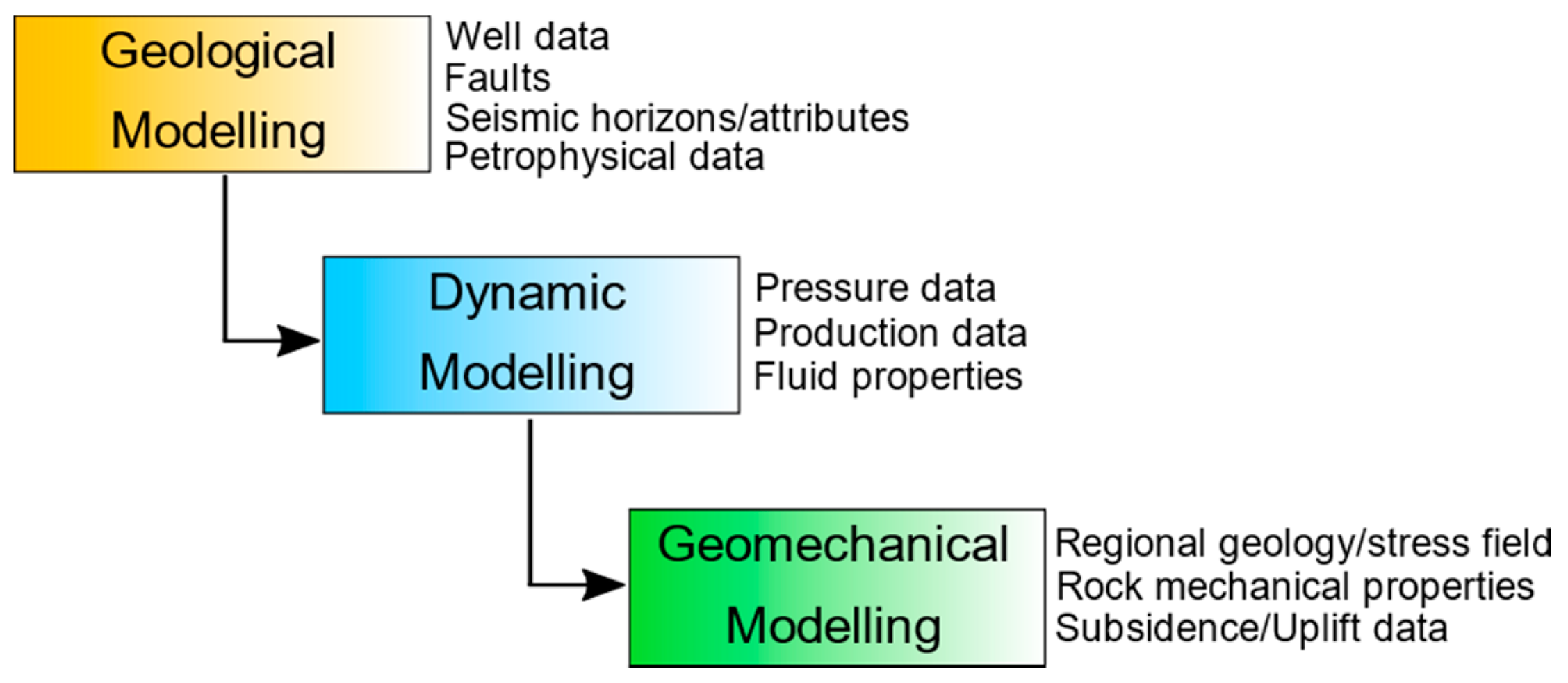
2. Materials and Methods
3. Results
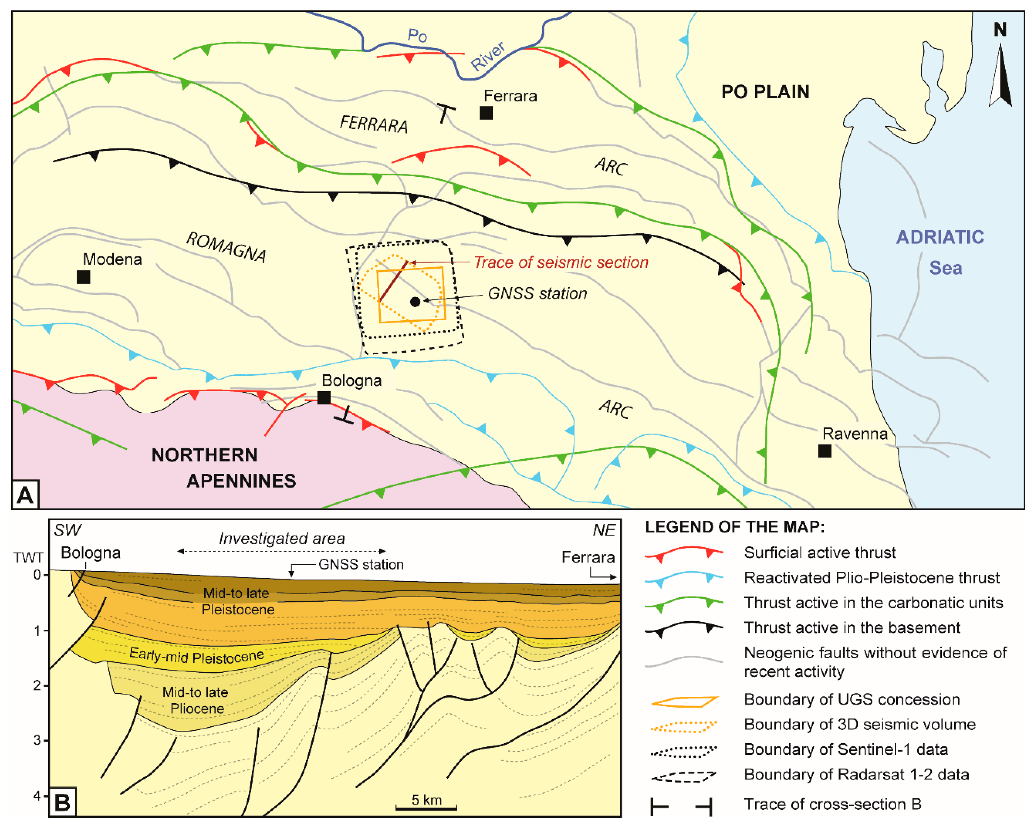
3.1. Regional Geological Setting
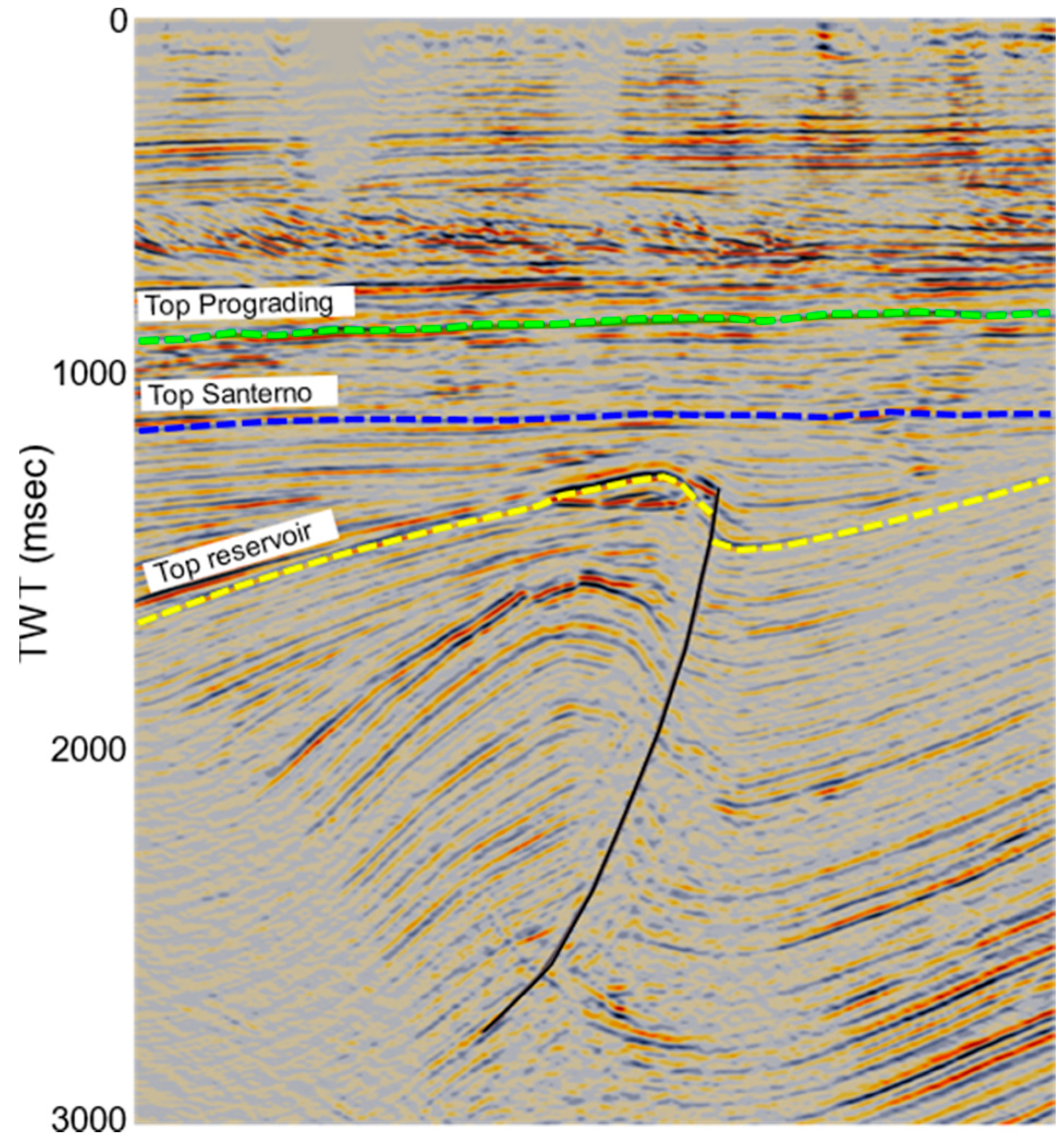
3.2. UGS Gas Field Description
3.3. Ground Surface Monitoring Results
3.3.1. SAR interferometry results
3.3.2. GNSS results
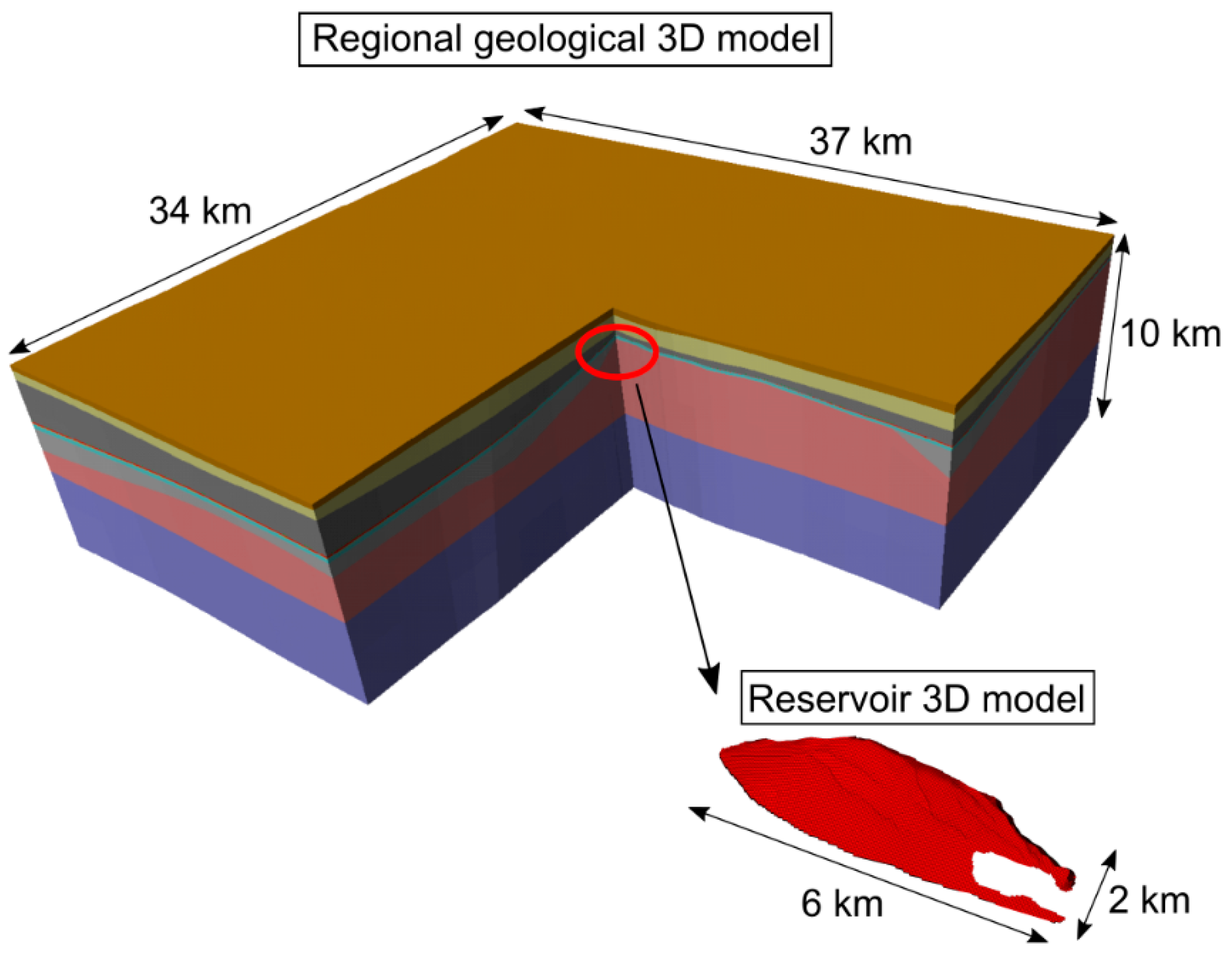
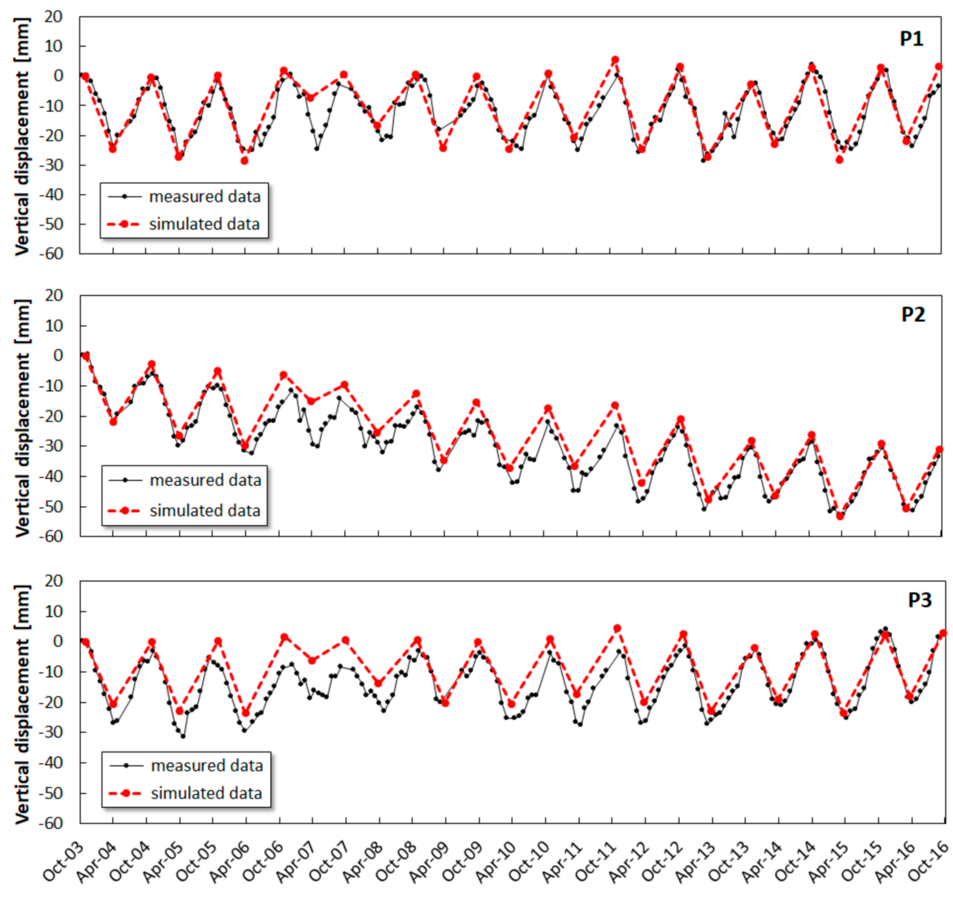
3.4. Geomechanical Simulation Results
4. Discussion
4.1. Ground Monitoring Data and Comparison with UGS
- (i)
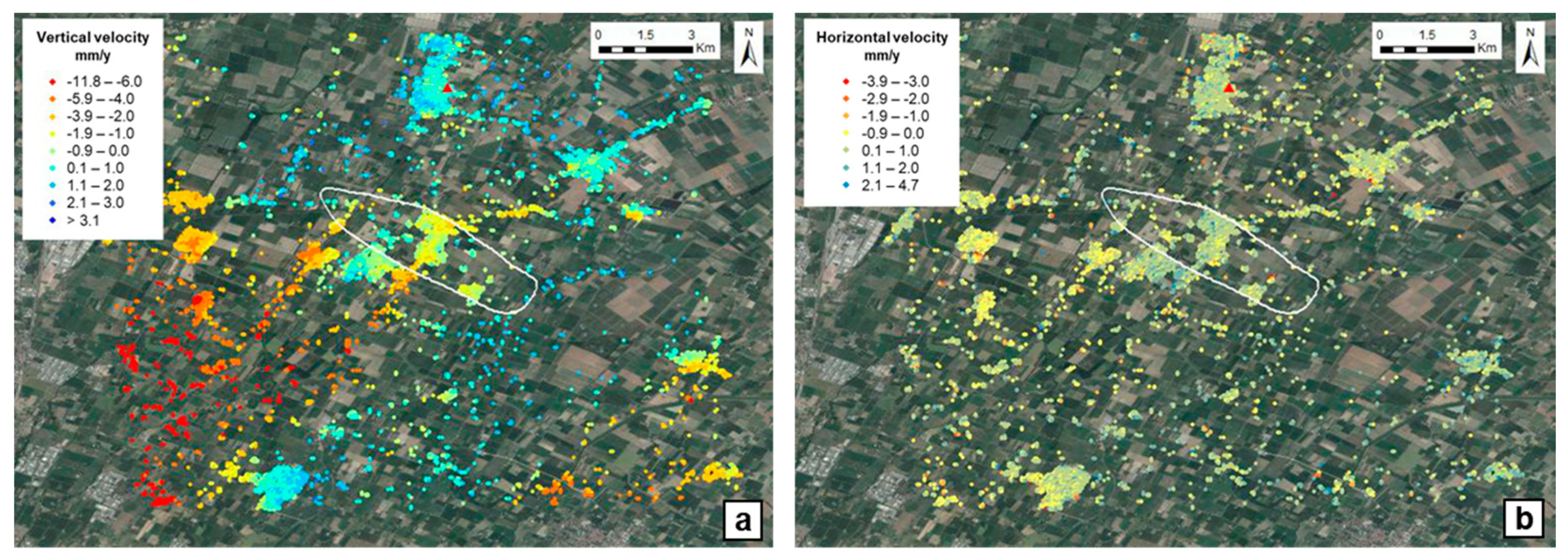
- the field area is characterized by a general long-term, gentle subsidence trend with no uplift evidence above the blind thrust, potentially ascribable to the growth of the buried anticline; a pronounced subsidence occurs in the direction of the Bologna city, outside the field area;
- (ii)
- the UGS activity does not affect the mean horizontal and vertical displacement velocities in the gas field area, which are coherent with the velocity range within the entire monitored domain;
- (iii)
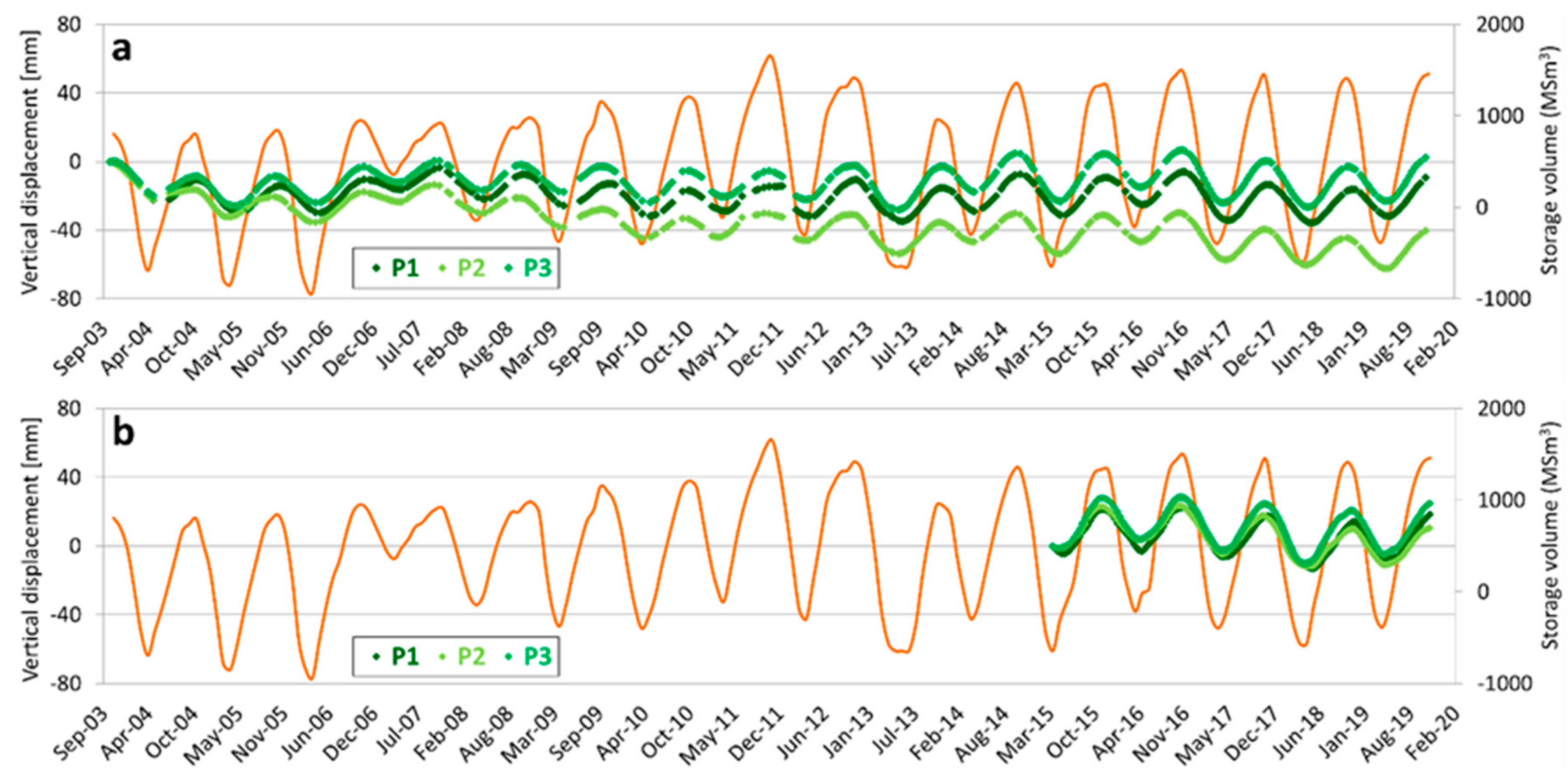
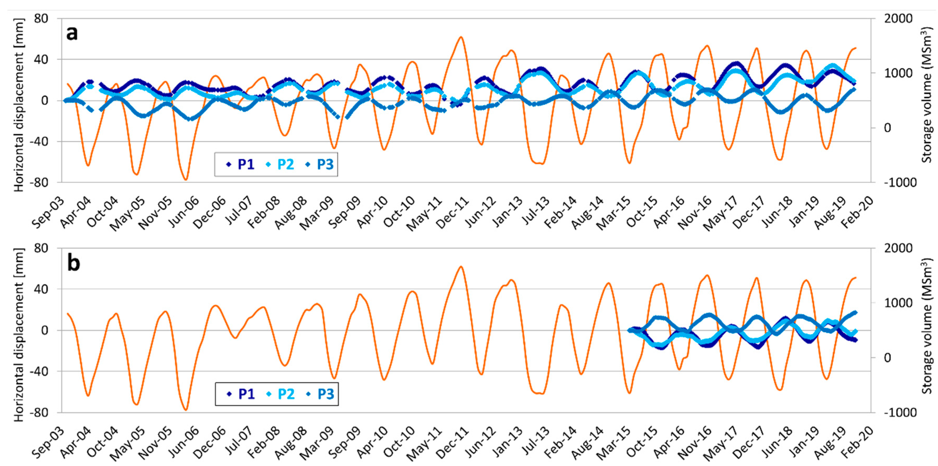
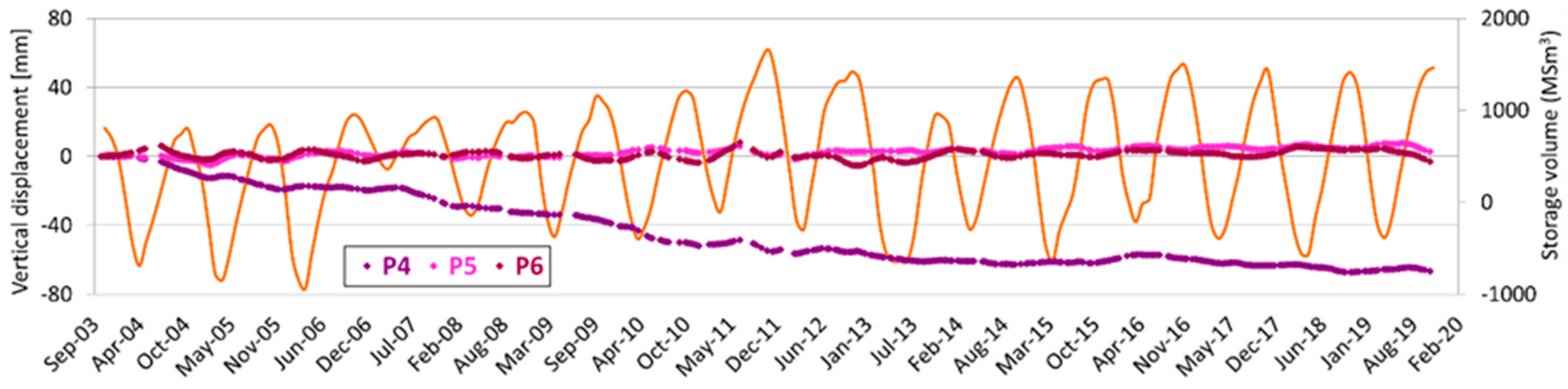
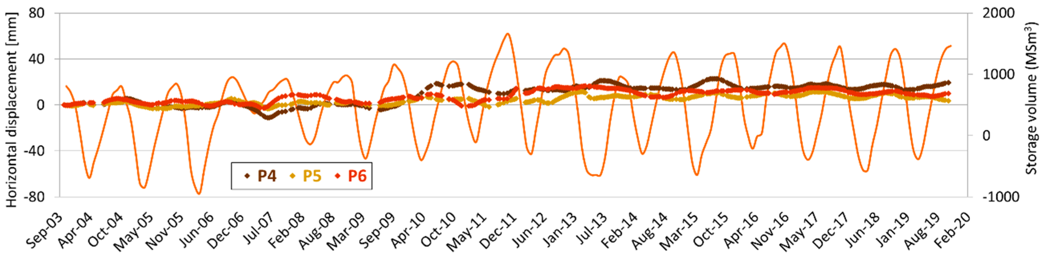
- a strong correlation exists between the curve of the storage gas cumulative volumes and the historical series of the ground displacement above the reservoir, considering both the vertical and East–West planar components;
- (iv)
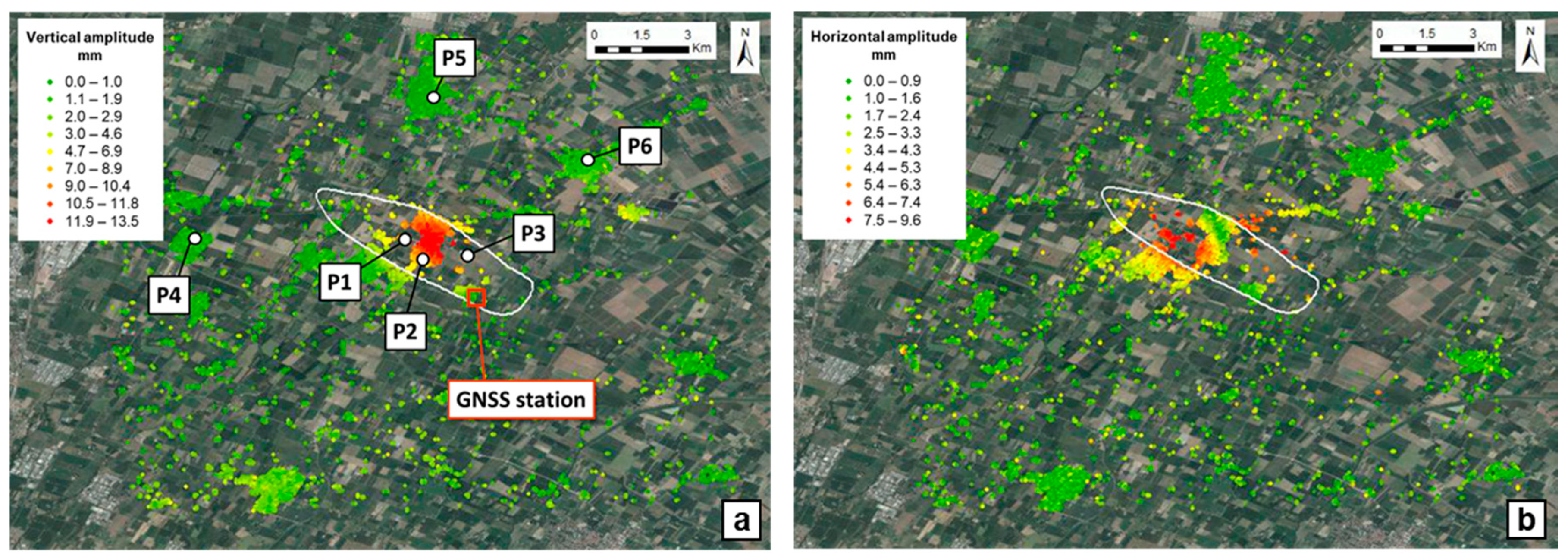
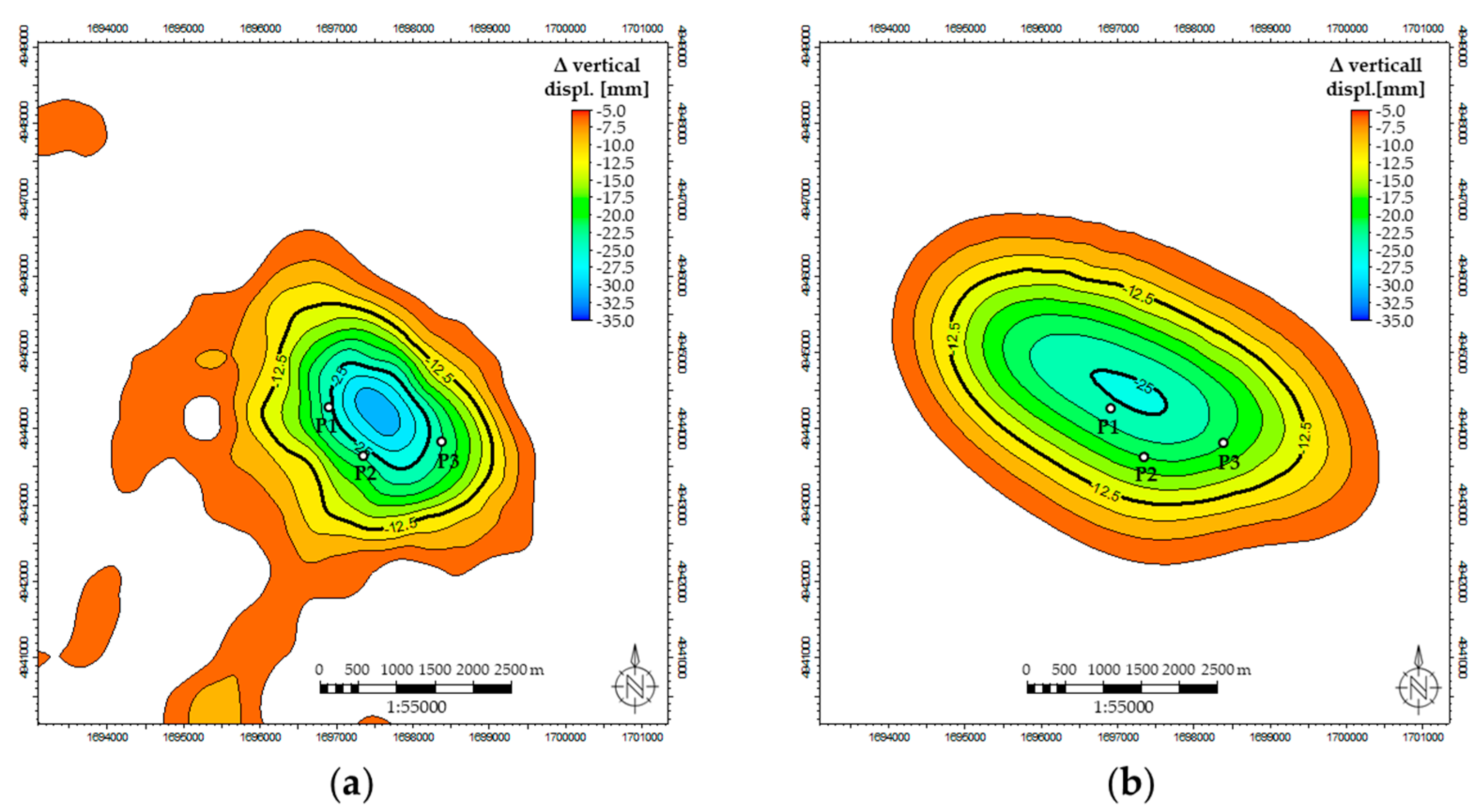
- the UGS-related, short-term, cyclical subsidence/uplift is limited to the field area; it is maximum in the center of the area while it dissipates near the field boundary.
- (i)
- the GNSS site is characterized by a long-term, gentle subsidence trend, in agreement with InSAR data;
- (ii)
- the estimated areal velocities are consistent with the NE-ward vergence of the Northern Apennines driven by the movement of the Eurasiatic plate (e.g., [35]);
- (iii)
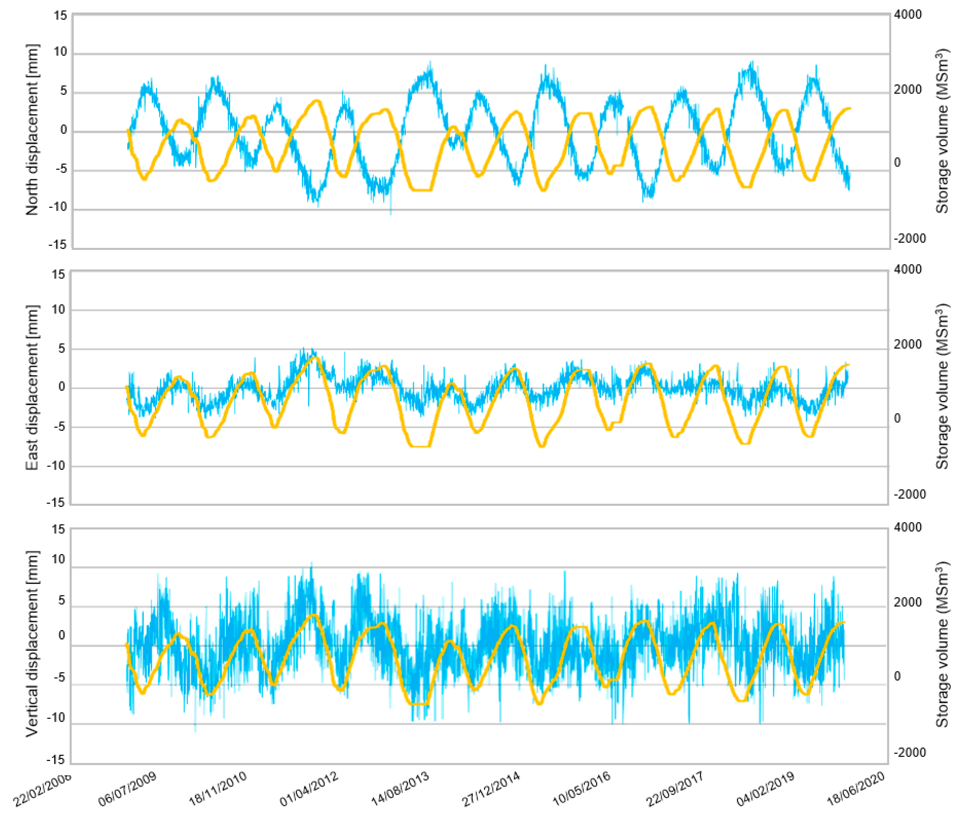
- The short-term, seasonal vertical displacement of the GNSS station (placed close to the field boundary) is largely due to the variation in hydrological load rather than the UGS activities, resulting in the absence of an appreciable correlation between the curve of the storage gas cumulative volumes and the residual sinusoidal trend. The GNSS response is coherent with InSAR data, which show the decrease in the UGS-related cyclical vertical displacement towards the field boundary;
- (iv)
- a strong correlation exists between the UGS activities and the short-term, seasonal horizontal displacements; in particular, the GNSS station is more sensitive to the North–South planar component of movement due to its location at the south-eastern edge of the gas field area.
4.2. Discussion about the Geomechanical Simulation Results
5. Conclusions
Author Contributions
Funding
Acknowledgments
Conflicts of Interest
References
- Poland, J.F.; Davis, G.H. Land Subsidence Due to Withdrawal of Fluids. Rev. Eng. Geol. 1969, 2, 187–270. [Google Scholar] [CrossRef]
- Settari, A.; Walters, D.A.; Stright, D.H.; Aziz, K. Numerical Techniques Used for Predicting Subsidence Due to Gas Extraction in the North Adriatic Sea. Pet. Sci. Technol. 2008, 26, 1205–1223. [Google Scholar] [CrossRef]
- Rutqvist, J.; Vasco, D.W.; Myer, L.R. Coupled reservoir-geomechanical analysis of CO2 injection and ground deformations at In Salah, Algeria. Int. J. Greenh. Gas Control. 2010, 4, 225–230. [Google Scholar] [CrossRef] [Green Version]
- Giani, G.; Orsatti, S.; Peter, C.; Rocca, V. A Coupled Fluid Flow—Geomechanical Approach for Subsidence Numerical Simulation. Energies 2018, 11, 1804. [Google Scholar] [CrossRef] [Green Version]
- Casero, P. Structural setting of petroleum exploration plays in Italy. In Italian Geological Societ Special Volume for the 32nd IGC, 20–28 August 2004, Florence, Italy; Società geologica italiana (Italian Geological Society): Rome, Italy, 2004; pp. 188–189. [Google Scholar]
- Baú, D.; Gambolati, G.; Teatini, P. Residual land subsidence near abandoned gas fields raises concern over northern Adriatic coastland. EOS Trans. Am. Geoph. Union 2000, 81, 245. [Google Scholar] [CrossRef]
- Baú, D.; Ferronato, M.; Gambolati, G.; Teatini, P. Basin-scale compressibility of the northern Adriatic by the radioactive marker technique. Geotechnique 2002, 52, 605–616. [Google Scholar]
- Teatini, P.; Ferronato, M.; Gambolati, G.; Gonella, M. Groundwater pumping and land subsidence in the Emilia-Romagna coastland, Italy: Modeling the past occurrence and the future trend. Water Resour. Res. 2006, 42, 01406. [Google Scholar] [CrossRef]
- Dacome, M.C.; Miandro, R.; Vettorel, M.; Roncari, G. Subsidence monitoring network: An Italian example aimed at a sustainable hydrocarbon E&P activity. In Proceedings of the International Association of Hydrological Sciences (IAHS), Nagoya, Japan, 15–19 November 2015; Copernicus GmbH: Göttingen, Germany, 2015; Volume 372, pp. 379–384. [Google Scholar] [CrossRef] [Green Version]
- Benetatos, C.; Codegone, G.; Deangeli, C.; Giani, G.; Gotta, A.; Marzano, F.; Rocca, V.; Verga, F. Guidelines for the Study of Subsidence Triggered by Hydrocarbon Production; GEAM—Geoingegneria Ambientale e Mineraria Anno LIV: Turin, Italy, 2017; Volume 3, pp. 85–96, ISSN 11219041. [Google Scholar]
- Coti, C.; Rocca, V.; Sacchi, Q. Pseudo-Elastic Response of Gas Bearing Clastic Formations: An Italian Case Study. Energies 2018, 11, 2488. [Google Scholar] [CrossRef] [Green Version]
- Castelletto, N.; Ferronato, M.; Gambolati, G.; Janna, C.; Teatini, P.; Marzoati, D.; Cairo, E.; Colombo, D.; Feretti, A.; Bagliani, A.; et al. 3D geomechanics in UGS projects. A comprehensive study in Northern Italy. In Proceedings of the 44th US Rock Mechanics Symposium and 5th U.S.—Canada Rock Mechanics Symposium, Salt Lake City, UT, USA, 27–30 June 2010; pp. 27–30. [Google Scholar]
- Fjær, E.; Holt, R.; Horsrud, P.; Raaen, A.; Risnes, R. Chapter 3 Geological aspects of petroleum related rock mechanics. In Developments in Petroleum Science, 2nd ed.; Elsevier BV: Amsterdam, The Netherlands, 2008; Volume 53, pp. 103–133. [Google Scholar]
- Costantini, M.; Falco, S.; Malvarosa, F.; Minati, F.; Trillo, F. Method of persistent scatterer pairs (PSP) and high resolution SAR interferometry. In Proceedings of the 2009 IEEE International Geoscience and Remote Sensing Symposium (IGARSS ’09), Cape Town, South Africa, 12–17 July 2009; Volume 3, pp. 904–907. [Google Scholar]
- Costantini, M.; Malvarosa, F.; Minati, F.; Vecchioli, F. Multi-scale and block decomposition methods for finite difference integration and phase unwrapping of very large datasets in high resolution SAR interferometry. Geosci. Remote Sens. Symp. IEEE Int. 2012, 5574–5577. [Google Scholar] [CrossRef]
- Costantini, M.; Malvarosa, F.; Minati, F. A General Formulation for Redundant Integration of Finite Differences and Phase Unwrapping on a Sparse Multidimensional Domain. IEEE Trans. Geosci. Remote Sens. 2011, 50, 758–768. [Google Scholar] [CrossRef]
- Costantini, M.; Falco, S.; Malvarosa, F.; Minati, F.; Trillo, F.; Vecchioli, F. Persistent Scatterer Pair Interferometry: Approach and Application to COSMO-SkyMed SAR Data. IEEE J. Sel. Top. Appl. Earth Obs. Remote Sens. 2014, 7, 2869–2879. [Google Scholar] [CrossRef]
- Dach, R.; Lutz, S.; Walser, P.; Fridez, P. (Eds.) Bernese GNSS Software Version 5; AIUB-Astronomical Institute, University of Bern: Bern, Switzerland, 2015. [Google Scholar]
- Codegone, G.; Rocca, V.; Verga, F.; Coti, C. Subsidence Modeling Validation Through Back Analysis for an Italian Gas Storage Field. Geotech. Geol. Eng. 2016, 34, 1749–1763. [Google Scholar] [CrossRef]
- Teatini, P.; Castelletto, N.; Ferronato, M.; Gambolati, G.; Janna, C.; Cairo, E.; Marzorati, D.; Colombo, D.; Ferretti, A.; Bagliani, A.; et al. Geomechanical response to seasonal gas storage in depleted reservoirs: A case study in the Po River basin, Italy. J. Geophys. Res. Space Phys. 2011, 116. [Google Scholar] [CrossRef]
- Ferronato, M.; Castelletto, N.; Gambolati, G.; Janna, C.; Teatini, P. II cycle compressibility from satellite measurements. Géotechnique 2013, 63, 479–486. [Google Scholar] [CrossRef]
- Pieri, M.; Groppi, G. Subsurface Geological Structure of the Po Plain, Italy. In Progetto Finalizzato Geodinamica; Consiglio Nazionale Delle Ricerche: Rome, Italy, 1981; Volume 414, pp. 1–13. [Google Scholar]
- Fantoni, R.; Franciosi, R. Tectono-sedimentary setting of the Po Plain and Adriatic foreland. Rend. Lince 2010, 21, 197–209. [Google Scholar] [CrossRef]
- Ghielmi, M.; Minervini, M.; Nini, C.; Rogledi, S.; Rossi, M.; Vignolo, A. Sedimentary and tectonic evolution in the eastern Po-Plain and northern Adriatic Sea area from Messinian to Middle Pleistocene (Italy). Rend. Lince 2010, 21, 131–166. [Google Scholar] [CrossRef]
- Amadori, C.; Toscani, G.; Di Giulio, A.; Maesano, F.E.; D’Ambrogi, C.; Ghielmi, M.; Fantoni, R. From cylindrical to non-cylindrical foreland basin: Pliocene–Pleistocene evolution of the Po Plain–Northern Adriatic basin (Italy). Basin Res. 2019, 31, 991–1015. [Google Scholar] [CrossRef] [Green Version]
- Turrini, C.; Toscani, G.; Lacombe, O.; Roure, F. Influence of structural inheritance on foreland-foredeep system evolution: An example from the Po valley region (northern Italy). Mar. Pet. Geol. 2016, 77, 376–398. [Google Scholar] [CrossRef]
- Carminati, E.; Doglioni, C. Alps vs. Apennines: The paradigm of a tectonically asymmetric Earth. Earth-Sci. Rev. 2012, 112, 67–96. [Google Scholar] [CrossRef]
- Toscani, G.; Bonini, L.; Ahmad, M.I.; Di Bucci, D.; Di Giulio, A.; Seno, S.; Galuppo, C. Opposite verging chains sharing the same foreland: Kinematics and interactions through analogue models (Central Po Plain, Italy). Tectonophisics 2014, 633, 268–282. [Google Scholar] [CrossRef]
- Bigi, G.; Castellarin, A.; Coli, M.; Dal Piaz, G.V.; Sartori, R.; Scandone, P. Structural Model of Italy Sheet 1, 1:Progetto Finalizzato Geodinamica; Consiglio Nazionale delle Ricerche: SELCA Firenze, Italy, 1990. [Google Scholar]
- Boccaletti, M.; Bonini, M.; Corti, G.; Gasperini, P.; Martelli, L.; Piccardi, L.; Severi, P.; Vannucci, G. Seismotectonic Map of the Emilia-Romagna Region; Emilia-Romagna Region-SGSS and CNRIGG: Florence, Italy, 2004. [Google Scholar]
- Boccaletti, M.; Corti, G.; Martelli, L. Recent and active tectonics of the external zone of the Northern Apennines (Italy). Acta Diabetol. 2010, 100, 1331–1348. [Google Scholar] [CrossRef]
- Ghielmi, M.; Minervini, M.; Nini, C.; Rogledi, S.; Rossi, M. Late Miocene–Middle Pleistocene sequences in the Po Plain—Northern Adriatic Sea (Italy): The stratigraphic record of modification phases affecting a complex foreland basin. Mar. Pet. Geol. 2013, 42, 50–81. [Google Scholar] [CrossRef]
- Dong, D.; Fang, P.; Bock, Y.; Cheng, M.K.; Miyazaki, S. Anatomy of apparent seasonal variations from GPS-derived site position time series. J. Geophys. Res. Space Phys. 2002, 107, 2075. [Google Scholar] [CrossRef] [Green Version]
- Gelaro, R.; Mccarty, W.; Suárez, M.J.; Todling, R.; Molod, A.; Takacs, L.; Randles, C.A.; Darmenov, A.; Bosilovich, M.G.; Reichle, R.H.; et al. The Modern-Era Retrospective Analysis for Research and Applications, Version 2 (MERRA-2). J. Clim. 2017, 30, 5419–5454. [Google Scholar] [CrossRef] [PubMed]
- ARPAE (Agenzia Prevenzione Ambientale Energia Emilia-Romagna). Rilievo Della Subsidenza Nella Pianura Emiliano-Romagnola Seconda Fase, Bologna; ARPAE: Bologna, Italy, 2018; p. 105. [Google Scholar]
- Bitelli, G.; Bonsignore, F.; Del Conte, S.; Franci, F.; Lambertini, A.; Novali, F.; Severi, P.; Vittuari, L. Updating the subsidence map of Emilia-Romagna region (Italy) by integration of SAR interferometry and GNSS time series: The 2011–2016 period. Proc. IAHS 2020, 382, 39–44. [Google Scholar] [CrossRef] [Green Version]
- Dobereiner, L. Engineering Geology of Weak Sandstones. Ph.D. Thesis, University of London, London, UK, 1984. [Google Scholar]
- Kanji, M.A. Critical issues in soft rocks. J. Rock Mech. Geotech. Eng. 2014, 6, 186–195. [Google Scholar] [CrossRef] [Green Version]
- Marzano, F.; Pregliasco, M.; Rocca, V. Experimental characterization of the deformation behavior of a gas-bearing clastic formation: Soft or hard rocks? A case study. Géoméch. Geophys. Geo-Energy Geo-Resour. 2019, 6, 10. [Google Scholar] [CrossRef]
- Rocca, V.; Cannata, A.; Gotta, A. A critical assessment of the reliability of predicting subsidence phenomena induced by hydrocarbon production. Géoméch. Energy Environ. 2019, 20, 100129. [Google Scholar] [CrossRef]


| Feature | Network Approach | Precise Point Positioning Approach |
|---|---|---|
| Software | Bernese v. 5.2 | Bernese v. 5.2 |
| Each process time span | Daily arc (daily RINEX) | Daily arc (daily RINEX) |
| Observables | Double Difference | One-way |
| GNSS Ephemerides; ERP | Final IGS | Final IGS |
| Clock Correction | Not strictly required (Final IGS CLK) | Final IGS CLK (Mandatory) |
| Tropospheric Modeling | Neill Mapping Function | Vienna Mapping Function (VMF) |
| Terrestrial Reference Frame | ITRF2014 | Forced by the Orbits |
| Reference Stations in the process | BUCU, GRAS, GRAZ, MATE, MEDI, NOT1, SOFI, WTZR, ZIMM | No one |
| Formations | Geomechanical Classes | E | ν | ρ | β | c | φ | Tensile Cut-Off |
|---|---|---|---|---|---|---|---|---|
| [GPa] | [-] | [g/cm3] | [-] | [105 Pa] | [°] | [105 Pa] | ||
| Alluvium | 1 | 0.3 | 0.39 | 2.20 | 1 | 4 | 38 | 4 |
| Asti sand | 2 | 0.5 | 0.39 | 2.10 | 1 | 4 | 36 | 4 |
| Santerno clay | 3 | 5.2 | 0.39 | 2.18 | 1 | 15 | 20 | 15 |
| 4 | 5.0 | 0.39 | 2.18 | 1 | 15 | 20 | 15 | |
| Santerno clay/P.to Garibaldi sand | 5 | 6.0 | 0.39 | 2.20 | 1 | 12 | 35 | 12 |
| 6 | 6.3 | 0.39 | 2.18 | 1 | 15 | 20 | 15 | |
| P.to Garibaldi sand | 7 | 8.0 | 0.39 | 2.18 | 1 | 15 | 20 | 15 |
| Santerno clay | 8 | 9.5 | 0.39 | 2.20 | 1 | 20 | 24 | 20 |
| 9 | 11.0 | 0.39 | 2.20 | 1 | 20 | 24 | 20 | |
| 10 | 12.9 | 0.39 | 2.20 | 1 | 20 | 24 | 20 | |
| P.to Corsini sand | 11 | 15.7 | 0.39 | 2.40 | 1 | 10 | 35 | 10 |
| 12 | 19.6 | 0.39 | 2.40 | 1 | 20 | 35 | 20 | |
| 13 | 25.3 | 0.39 | 2.40 | 1 | 30 | 35 | 30 | |
| Basal formation | 14 | 35.0 | 0.39 | 2.40 | 1 | 50 | 35 | 50 |
| Satellite | Observation Geometry | Scene | Time Interval |
|---|---|---|---|
| RSAT1 | Ascending right | 118 | 16/10/2003–09/03/2013 |
| RSAT1 | Descending right | 104 | 03/10/2003–20/03/2013 |
| RSAT2 | Ascending right | 87 | 21/11/2012–16/10/2019 |
| RSAT2 | Descending right | 92 | 25/04/2013–27/10/2019 |
| S1 | Ascending right | 227 | 30/03/2015–29/10/2019 |
| S1 | Descending right | 232 | 24/10/2014–28/10/2019 |
Publisher’s Note: MDPI stays neutral with regard to jurisdictional claims in published maps and institutional affiliations. |
© 2020 by the authors. Licensee MDPI, Basel, Switzerland. This article is an open access article distributed under the terms and conditions of the Creative Commons Attribution (CC BY) license (http://creativecommons.org/licenses/by/4.0/).
Share and Cite
Benetatos, C.; Codegone, G.; Ferraro, C.; Mantegazzi, A.; Rocca, V.; Tango, G.; Trillo, F. Multidisciplinary Analysis of Ground Movements: An Underground Gas Storage Case Study. Remote Sens. 2020, 12, 3487. https://0-doi-org.brum.beds.ac.uk/10.3390/rs12213487
Benetatos C, Codegone G, Ferraro C, Mantegazzi A, Rocca V, Tango G, Trillo F. Multidisciplinary Analysis of Ground Movements: An Underground Gas Storage Case Study. Remote Sensing. 2020; 12(21):3487. https://0-doi-org.brum.beds.ac.uk/10.3390/rs12213487
Chicago/Turabian StyleBenetatos, Christoforos, Giulia Codegone, Carmela Ferraro, Andrea Mantegazzi, Vera Rocca, Giorgio Tango, and Francesco Trillo. 2020. "Multidisciplinary Analysis of Ground Movements: An Underground Gas Storage Case Study" Remote Sensing 12, no. 21: 3487. https://0-doi-org.brum.beds.ac.uk/10.3390/rs12213487