Measuring and Monitoring Urban Impacts on Climate Change from Space


1
CropSnap LLC, Sunnyvale, CA 94087, USA
2
Foothill College, Los Altos Hills, CA 94022, USA
3
Potsdam Institute for Climate Impact Research, 14473 Potsdam, Germany
*
Author to whom correspondence should be addressed.
Remote Sens. 2020, 12(21), 3494; https://0-doi-org.brum.beds.ac.uk/10.3390/rs12213494
Submission received: 31 July 2020
/
Revised: 13 October 2020
/
Accepted: 22 October 2020
/
Published: 24 October 2020
(This article belongs to the Special Issue Remote Sensing based Urban Development and Climate Change Research)
Abstract
:As urban areas continue to expand and play a critical role as both contributors to climate change and hotspots of vulnerability to its effects, cities have become battlegrounds for climate change adaptation and mitigation. Large amounts of earth observations from space have been collected over the last five decades and while most of the measurements have not been designed specifically for monitoring urban areas, an increasing number of these observations is being used for understanding the growth rates of cities and their environmental impacts. Here we reviewed the existing tools available from satellite remote sensing to study urban contribution to climate change, which could be used for monitoring the progress of climate change mitigation strategies at the city level. We described earth observations that are suitable for measuring and monitoring urban population, extent, and structure; urban emissions of greenhouse gases and other air pollutants; urban energy consumption; and extent, intensity, and effects on surrounding regions, including nearby water bodies, of urban heat islands. We compared the observations available and obtainable from space with the measurements desirable for monitoring. Despite considerable progress in monitoring urban extent, structure, heat island intensity, and air pollution from space, many limitations and uncertainties still need to be resolved. We emphasize that some important variables, such as population density and urban energy consumption, cannot be suitably measured from space with available observations.

1. Introduction
Emissions of greenhouse gases (GHG) as well as other short-lived atmospheric pollutants from burning fossil fuels together with land use change are the major reasons behind climate change, and fast-paced urbanization is increasingly being identified as the major culprit. Today, urban areas host more than half of the global population and are responsible for over 70% of the global GHG emissions from final energy use [1]. In addition to global warming trends, urban areas experience a local urban heat island (UHI) effect resulting from the high density of impervious surfaces, modification of air ventilation from built-up structures, as well as waste heat emissions from residential and industrial sources [2]. Moreover, high air temperatures interact with urban air pollution in multiple ways. For example, higher temperatures modify the distribution of pollutants in the air [3,4] and influence intensity and frequency of rainfall over some cities [5]. A further increase in temperatures can exacerbate these effects. Additionally, air pollutants such as particulate matter have an effect on radiative forcing, modifying scattering and absorption of solar radiation. Rising temperatures also increase biogenic emissions of volatile organic compounds and the speed of their reaction with nitrogen oxides leading to enhanced ground level ozone production [6]. UHI, urban air pollution, and their interaction have local to regional effects on the surface energy balance (regional warming, accelerated water cycle, modified rainfall patterns), while GHG emissions and changes in surface albedo resulting from urban expansion have global impacts.
The population and extent of cities continue to grow. The area of global cities is projected to triple globally from 2000 to 2030 [7]. Urban development increases demand for water, energy, construction materials, and food. Quantitative analysis of the global resource requirements of cities indicated that without a new approach to urbanization, material consumption by the world’s cities will grow from 40 billion tons in 2010 to about 90 billion tons by 2050 [8]. Cities use billions of tons of raw materials, from fossil fuels, sand, gravel, and iron ore, to biotic resources such as wood and food. At the same time, changes in climate such as in regional precipitation patterns, storm frequency and severity, snowmelt timing, and heat waves have already started to affect or even disrupt the supply and storage of these resources (e.g., [9]). In addition to increased burden on resources, urban growth consumes vast areas of valuable agricultural land and threatens biological diversity through habitat fragmentation. Increased demand for energy and loss of natural spaces will also likely exacerbate climate change. Many cities are coastal and their dwellers are already facing the challenges of adaptation to sea level rise, increased storm frequency, and enhanced flooding [10]. Cities located in floodplains are at increased risk of flooding from the intensification of storm events [11].
Monitoring urban areas from space offers the advantage of broad coverage, synoptic, repeated observations, and the ability to measure consistently important physical properties with well-validated methods. Through long-term observations from space, relevant variables can be analyzed over time and across scales, also making it possible to understand relationships between the changes brought by urban expansion in terms of land cover, climate, and pollutant emissions and the surrounding regions and improve the possibility of objective comparisons across time, geographies, and socio-economic and policy settings [12].
Remote sensing capabilities are now available from a variety of sensors and at different temporal and spatial resolutions to either measure directly physical variables with significance to the urban issues linked to climate change or provide suitable proxies. Available remote sensing technologies range from optical, thermal infrared, microwave (including radar, scatterometers, and altimeters), as well as light detection and ranging (LiDAR). Variables that can be obtained from space observation are needed for monitoring major issues that can be measured at city scales: Urban population, extent, and structure, urban energy consumption, urban emissions of GHG and other air pollutants, extent and intensity of surface UHI (SUHI) effect (Table 1). These issues are interrelated in complex ways (Figure 1) and some of the remote sensing capabilities can be used to measure more than one variable and address multiple issues. Most of the global populations now live in urban areas [13], drive the demand for land (urban extent) and, with their densities, shape the urban structure [14,15]. Urban population growth also drives the demand for energy and resources [16]. Urban extent and structure are among the major determinants of land use change around cities. Urban-driven land use changes, accompanied by many demographic and economic changes, strongly impact the regional physical and biogeochemical properties of the earth, and have consequences on energy use (for cooling and heating of buildings, lighting, appliance use, and transportation), the emissions of GHG (the majority of global emissions are attributed to cities), and other air pollutants [17]. Urban structure and extent also impact the strength of the UHI and excess urban heat in general, although in complex ways [18], which then feeds back on additional energy use for cooling and additional GHG and air pollutants emissions [19]. Air pollutants, whose concentrations are largely related to energy use and urban size and structure, can shape the climate of individual cities in complex ways [6] and adversely impact human health.
Remote sensing technologies can contribute to monitoring, testing, and exploring solutions for evolving urban development to adapt to and to mitigate the changing climate. Wentz et al. [20] reviewed capabilities of remotely sensed earth observations for mapping and modelling global environmental change research with a special focus on urbanization. Zhou et al. [21] focused their efforts on reviewing the state of the art in SUHI research from space. Prakash et al. [22] discussed the opportunities offered by open-source remote-sensing technologies for sustainable urban planning and decision making and shed light on the challenges that have to be overcome for wider adoption of these observations by city authorities. These challenges are not only technical skills needed for processing and interpretation of remotely sensed data, or the large data volumes, but also the high costs of high-resolution satellite images available from commercial sensors and LiDAR [23].
With the growth of urban areas and pronounced feedbacks between urbanization and global warming, cities are becoming the battleground for climate change mitigation, increasing the need for tools for the consistent monitoring of the implementation of mitigation measures. Here we review the existing tools available from satellite remote sensing to study urban contributions to climate change and that potentially could be used for monitoring the progress of climate change mitigation strategies at the city level.
2. Urban Population and Health
In 2007, the urban population reached half of the world population. Ever since, most of the population growth worldwide occurs in urban areas. It is estimated that about 55% of the world’s population now lives in urban areas. By midcentury it will be around 70%, including a surge in the number of megacities, which are agglomerations with populations of more than 10 million and largely located in developing countries [13]. Because most of the world’s population will live in cities in the decades ahead, estimating urban population and its dynamics are important for predicting demands for energy, materials, food, and other resources.
Census data can provide detailed maps of population distribution when they are linked with small-area administrative boundary data, such as zip-codes and census-blocks. However, the size of these boundaries can vary greatly depending on the population counts within them, and population may not be distributed homogeneously. As censuses are highly costly and, for various political and socio-economic reasons, difficult to be conducted accurately, they often do not offer up-to-date or reliable population counts, particularly where there are large informal settlements [24]. Population cannot be directly observed with current remote sensing technology but can be estimated from density of human settlement distribution and other covariates [24].
Historically, space remote sensing has been used to either directly estimate population size [25,26,27], or to spatially disaggregate or refine census estimates of population through statistical modeling [28,29,30]. This presupposes that reliable census data are available. Under the assumption that human population is associated with settlements, aggregated population counts can be spatially disaggregated with dasymetric mapping techniques, producing gridded population maps. Very high-resolution maps of built-up areas derived from Pleiades pansharpened data at 0.5 m for Dakar, Senegal, were shown to significantly improve the accuracy of spatial disaggregation compared to built-up extents at 10-m resolution from Landsat and Sentinel-2 data fusion [31].
With greater access to high-resolution satellite imagery and computing power, population maps are produced using settlement extent maps derived from satellite data and other covariates to train machine learning algorithms with population counts sampled from a range of socio-economic conditions. High-resolution maps of settlements in conjunction with micro census surveys have been shown to be effective at estimating population independently of the census in Nigeria, where existing census data are outdated and unreliable [32].
In dense urban settings with high-rise buildings, tri-dimensional variations in urban structure can complicate modeling population counts from simple masks of built-up extent; combining ortho-imagery from very high-resolution imagery with building volumes from LiDAR data or dasymetric mapping could help overcome this challenge [33,34]. However, these approaches have large uncertainties that have not yet been quantified. Uncertainties are associated with the false identification of building footprints and with the estimation of buildings’ occupancy rates.
To date, the Global Human Settlement Layer (GHSL) is the most accurate dataset for mapping the distribution of human population globally [35]. It was created using global and continental satellite image archives, fine-scale satellite imagery, census data, and volunteered geographic information. The dataset is available for the reference periods 1975, 1990, 2000, and 2015, with the population expressed as total number of people per 250-m grid cell (Figure 2). The major uncertainty in these datasets is, again, the strong interdependence of population counts on the correct identification of built-up structures.
Urban areas represent population hotspots with large consequences for increased public health concerns related to climate change, including increases in frequency and intensity of heat waves and other extreme events such as storms, floods, fires, and drought [36], and decreased food security [37,38]. Increases in temperature alone, which are more marked in urban areas because of the UHI effect, stress the body physiology, causing urban dwellers to be more likely to suffer from digestive diseases, nervous system issues, insomnia, depression, and mental illnesses (for example, [39,40]), with significant quality of life implications. Scores from the general health questionnaire-28 [41], a simple but reliable self-administered survey that is used to assess physical and mental health in the general population and within communities, were associated with intensifications of the SUHI effect in the metropolitan area of Isfahan, Iran, indicating that areas of the city that heated up more related to greater mental distress of the inhabiting population [42]. Cardiovascular, respiratory, and kidney diseases are also more common in hotter urban environments [43]. The incidence of numerous infectious diseases also presents climate correlates, such as relationships with temperature, humidity, and radiation [44,45,46]. In São Paulo, Brazil, land surface temperature data from Landsat data were found to be associated with increased breeding and blood feeding of Aedes aegypti mosquito, which transmits dengue fever and favors warmer and drier environments [47]. Increased urban temperatures were also found to be associated with greater West Nile infection rates in mosquitoes in the Chicago area, USA [48], and with greater spread of mosquitoes that can potentially become infected with malaria in the UK [49]. Environmental changes brought by urban land cover changes combined with greater proximity of people increases the spread of infectious diseases [50]. Accurate population density maps combined with spatial maps of various parameters that have implications for climate change adaptation and mitigation, such as high-resolution urban temperature maps, flood risk maps, and air pollution maps, therefore also have important public health applications. The design of the urban structure, including the siting of parks, green belts, community gardens, building alignment, but also medical facilities and cooling centers, should be planned with attention also to population distribution.
3. Urban Extent and Structure
Urban extent and its change over time are important determinants of the impact of urbanization on land and consequently on changes in climate. Urban extent not only increases because new urban dwellers need new housing and other infrastructures, but also because cities are becoming less compact over time. The long-term historic de-densification trend of two percent per year threatens to increase global urban land use from just below 1 million km2 to over 2.5 million km2 in 2050 [8]. Cities expand not only horizontally, but also in height. The number of supertall buildings (height > 200 m) increased by several orders of magnitude over the last century, from two in 1920 to almost 1600 in 2018 [51]. The conversion of land into paved urban areas dramatically changes the physical [52] and biogeochemical properties of the Earth surface. One of these changes involves the water and energy exchanges between the land surface and the atmosphere, and are the main determinants of the increases in surface temperatures of urbanized areas [53], responsible for the UHI and SUHI effects. A modeling study of potential urban expansion in Europe suggested that a 40% increase in urban area would double the region affected by thermal stress and significantly reduce summer precipitation [54].
Urban size also relates to resource consumption and economic activity [55], and alters the patterns of carbon sequestration potential of the land [56]. Greater urban areas require a larger infrastructure for roads and buildings and energy consumption. The greater the size, the greater the amount of energy used for construction, functioning of the city, economic activities, and transportation, resulting in greater carbon emissions. In addition to the horizontal extent, the vertical development of cities also relates to embodied and operational energy consumption [57,58].
Historically, remote sensing has been widely used for mapping urban extent along with other land cover types, from the use of aerial photography in the early days, to mapping based on Landsat data, to wall to wall to maps of global land cover. As earth observations became available for global urban mapping, such as from Moderate Resolution Imaging Spectroradiometer (MODIS), dedicated efforts to mapping urban land cover, rather all the types of land covers, became more common. Urban extent can now be derived from a number of satellites, with optical or synthetic aperture radar (SAR), at finer spatial resolution, some publicly available and increasingly commercially operated (Table 1).
The first global urban maps were first made possible with data from MODIS [59] and nighttime light emissions from the Defense Meteorological Program/Operational Line-Scan System (DMSP/OLS) [60]. As computational capacity and cloud computing platforms such as Google Earth Engine have become available and the free availability of medium-resolution data increased, first with the opening of the Landsat archive and later with the availability of Sentinel data, efforts at global urban mapping at decametric resolution (20 to 30 m) have become more common (e.g., [61,62]). The Global Human Settlement-BUILT dataset of global urban areas at 30 m was one of the first attempts at multitemporal global urban mapping using Landsat data and provides layers for the years 1975, 1990, 2000 and 2014 [63]. The Global Human Settlement-BUILT is currently being updated and improved with Sentinel-1 data and takes advantage of machine learning techniques training and classification techniques developed for big data [63]. A global multitemporal urban land map at 30 m [62] was produced consistently for multiple years from Landsat and DMSP/OLS data for the period 1990–2010 (at five years intervals). Although many techniques for urban landcover classification have been developed that perform well regionally, their global application is more uncertain [64]. The global multitemporal urban map applied a multi-step approach based on the Normalized Urban Areas Composite Index, which combines a binary mask obtained from the nighttime lights data from DMSP/OLS with the normalized difference vegetation index, normalized difference water index and the normalized difference built-up index calculated from Landsat data. Optical data still present many challenges in consistently distinguishing built-up material from bare soil and other non-constructed impervious materials such as fallow fields and bare rocks. Thus, new indices and classification algorithms are still being developed to address these limitations for mapping urbanization in arid and semi-arid regions (e.g., [65]). Another challenge of optical data for multi-temporal applications is the retrieval of suitable acquisitions over tropical areas, which are often covered by clouds. Alternative efforts for automated high-resolution global urban mapping are based on SAR data. To date, the highest spatial resolution urban extent map is from the Global Urban Footprint for reference year 2011, which was based on TanDEM-X and TerraSAR-X at 12-m resolution [23,66] (see an example in Figure 3). This dataset indicates that the total global built-up area in 2011 amounted to 834,260 km2, or about 0.64% of the Earth’s land surface [23], but is limited to a one-time assessment only. The public availability of SAR data from Sentinel-1, which has shown good potential for distinguishing urban areas based on their characteristics of consistently high backscatter, should provide the avenue for additional global multi-temporal urban datasets at fine spatial resolution in the near future [61]. Multi-temporal global and continental or regional urban extent products facilitate the consistent comparison across cities over space and over time, which often lead to better understanding of the processes that drive urbanization [67] and their consequences in terms of emissions. Finer-scale maps better capture the large heterogeneity in urban forms. While global studies mapping urban growth from space are still rare (e.g., [62]), satellite data are widely used to estimate local or regional rates of urban expansion [14]. The Atlas of Urban Expansion [68] is a publicly available collection of Landsat-derived data on quantity and quality of urban expansion (1990, 2000, and 2014) for 200 cities distributed worldwide that can be used to study the impacts of urban growth on climate related-issues. For example, it has been used to ascribe the increased air pollution (PM 2.5 and NO2 emissions) of 10 Chinese cities between 2000 and 2013 to urban sprawl [69]. With economic development, these Chinese cities have grown more fragmented and the dependency on car transportation has increased, leading to worsening air pollution. An analysis of land cover metrics on urban form calculated from the CORINE Land Cover data found that sprawl was responsible for greater GHG emissions in Europe [70]. Multi-temporal urban extent maps derived from Landsat data at five-year intervals for Chinese megacities also related expansion of urban land and the transportation network added to connect the newly urbanized land to increased CO2 emissions [71]. Eventually, an improved understanding of how urban size and growth relate to climate change issues will require also to develop geospatial methods for delineating the boundaries between urban and rural lands, as administrative definitions and built-up density criteria are often insufficient to satisfy research needs [72].
In addition to binary masks of urban extent (built-up vs. non built-up), recent efforts are geared towards a more complex understanding of the urban structure, which is related to the arrangement of the land use in urbanized areas, and which can be loosely defined as the combination of types of buildings (including height), road density, green and open spaces, and water bodies within urban areas [15,73]. The Local Climate Zones (LCZ) framework provides a protocol for the classification of these different types of structures that can be used to facilitate comparisons across different sites [18]. LCZs allow one to classify different types of urban and rural environments based on their effects on temperatures as they relate to their surface conditions. For example, rather than referring to an area as simply urban or rural, it assigns it to different built types (e.g., compact or open high-, mid- or low-rise, etc.) and different land cover types (e.g., dense or scattered trees, bare soil, or bare rock or paved, etc.). Such information on urban structure supports a better understanding of population distribution [74], GHG and other pollutants emissions [75,76], energy consumption [77], and the UHI and SUHI effects [78,79,80].
Thus far, studies of urban structure have been limited in scope, mostly focusing on the analysis of individual cities, mainly large metropolitan areas, and few have done multi-city comparisons (e.g., [81,82]). Larger comparisons are still missing, and a suitable framework needs to be defined to make them possible. This limitation is being addressed by the WUDAPT (World Urban Database and Access Portal Tool) project [83,84,85], a community effort that aims at providing urban scientists (and more particularly urban climatologists) with relevant information on urban forms and functions that are linked to LCZs. It also defends a global standardization of urban classification in the form of LCZs for comparing urban climate case studies between them. Finally, the parameters can be fed to urban climate models. Such tools can facilitate the generation of transferable solutions that can serve urban planning purposes. For instance, urban green spaces contribute to climate change mitigation both by taking up and storing carbon and by decreasing UHI effects. Location of urban vegetation, its structure, and carbon storage can be detected from space [86,87] and its other benefits estimated with additional numerical models [88].
Studies of the urban structure rely on resolving individual buildings and their heights. This is best done with very high-resolution commercial sensors and LiDAR data, which are still too expensive to be used at large scales [15]. The three-dimensional built-up infrastructure has been studied at coarse resolution at the global scale using backscatters from QuikSCAT SeaWinds microwave Scatterometer [89,90]. Li et al. [91] have developed a first model for large-scale mapping of urban heights using Sentinel-1 data and have tested the approach on large cities of the continental US. Because of the global availability of Sentinel-1 data, this approach has the potential to be adapted globally. The results are not as accurate as the ones that can be obtained from aerial LiDAR data or very high-resolution optical stereo images or TerraSAR-X data, which can separate individual buildings (for example, see [92,93]).
Information on urban extent and particularly structure are also required to assess the vulnerability of cities to natural hazards and manage the risks and adapt to changes, such as floods, which are expected to become more extreme [10,11]. Urban areas are vulnerable to flooding when they do not include enough pervious surfaces or are not equipped with an adequate storm drainage system [94]. With climate change, precipitation patterns can also change with more extreme downpours becoming more frequent [95]. The effects of extreme downpours can compound with increases in impervious areas. Remote sensing has been used to help assess flood risk, flood forecasting, and post-flood assessments. For example, remotely sensed impervious surface areas assessments can be used as input to hydrologic models [96]. While most of this work requires very accurate 3D modeling of terrain and building elevations, which relies on terrestrial or aerial LiDAR, space remote sensing has demonstrated some utility for managing flood risk. Although cloud-free optical data are usually not available immediately after a flood and there are challenges related to the complexity of SAR signals in urban settings, SAR data combined with Interferometric SAR (InSAR) coherence or with LiDAR data can be used to provide accurate high-resolution flood maps [97,98].
4. Energy Consumption
Heating and cooling of buildings, transportation, lighting, and various electrical appliances used by urban dwellers require energy. Global cities consume between 67 and 76% of global energy [1] and this consumption has been increasing over time. The energy consumption per capita increases with the rising affluence of urban dwellers [99]. Office buildings mainly use electricity for lights, equipment, heating, and cooling. Residential energy use is likely to vary considerably by climate. In temperate climates, most of the energy is used for indoor space and water heating, which currently depend more on fossil fuels [100]. Zoning of urban areas is needed for distinguishing residential from commercial use, since they have different patterns of energy use and different energy sources. If energy is generated from burning fossil fuels in the city, then energy use is correlated with CO2 emission levels. If renewable energy sources—e.g., hydro, solar, or wind—are used to generate energy, then CO2 emissions can be low even with high energy use per capita [101]. The implications of energy consumption for the global climate are highly dependent on the energy source.
Outdoor light emissions can be mapped with nighttime spectroradiometers. DMSP/OLS has been providing nighttime global light emission data in digital form from 1992 to 2013 at 1-km spatial resolution. With the launch of Suomi National Polar Partnership/Visible Infrared Imaging Radiometer Suite (VIIRS), global light emissions have been sensed with greater spatial detail (750 m) and radiometric resolution (14 bit). These data have been shown to correlate with electric power consumption at the national level [60] and at the subnational level, demonstrating that they can be used to predict interannual [102,103] and monthly [104] variations in electricity use in lower- and middle-income countries. To ascribe power use to individual cities or even metropolitan areas still presents challenges, especially because of the difficulty in delineating the boundaries of individual built-up areas [105].
Distinguishing different light sources, such as incandescent, fluorescent, or LED, which is not possible with DMSP/OLS and VIIRS and most nighttime sensors, as they are limited to panchromatic or visible multispectral bands, could more precisely indicate energy consumption [106]. Radiometric and spectral requirements that a nighttime sensor would need to distinguish lighting types have been assessed by de Meester and Storch [107]. The first source of visible multispectral nighttime space images have been provided by the International Space Station Astronaut photography program, which has been acquiring digital photography of the Earth’s night surface since 2001 [108] showing the different colors of outdoor artificial lights in different cities, and how they have changed as light energy saving and climate adaptation programs are being implemented. Sub-meter nighttime acquisitions are now possible with commercial satellites such as Jilin-1 and EROS-B (Table 1).
5. Emissions of GHG
Three-quarters of global GHG emissions are attributed to urban areas [1]. If the top 50 emitting cities were counted as one country, that ‘nation’ would rank third in emissions behind China and the United States [109]. Many cities are taking steps to combat climate change and set up targets for reducing their emissions of CO2. A 2014 survey lists 228 global cities—representing nearly half a billion people—that have pledged reductions equivalent to 454 megatons of CO2 [110]. There are similar pledges for other air pollutants. Cities have two types of emissions: Direct emissions from urban energy consumption activities and upstream emissions, i.e., emissions that occur along the global production chain of the goods and services purchased by urban dwellers. Although upstream emissions from urban households are in the same order of magnitude as cities’ overall direct emissions [111], we focus here on the direct emissions only. Can remotely sensed data collected from space provide capability to monitor the progress that cities make in reducing their emissions of GHG?
There are currently a few satellite instruments that are able to detect the number of molecules of a particular gas between the instrument and the Earth’s surface—a vertical column density in units of molecules per unit area of the Earth’s surface (Table 1). If gas transport, deposition, and chemical conversion are minimal or are accounted for, then the observation can reflect the emission rate of that gas. Satellite sensors that detect CO2 dry air mole fraction (XCO2) in an air column are useful for monitoring direct emissions of CO2 and other GHG from cities [112,113]. The first space measurements that focused on XCO2 were from Scanning Imaging Absorption Spectrometer for Atmospheric Cartography (SCIAMACHY) on ENVISAT, which was active over the period 2002–2012. With data from SCIAMACHY, regional XCO2 enhancements related to yearly changes in anthropogenic CO2 emissions were detected from industrial areas in Germany, the East Coast of the United States, and the Yangtze River Delta [114]. SCIAMACHY had coarse spatial resolution (∼ 60 km × 30 km) and low sensitivity (~4–8 ppm). It was used only to detect large emissions enhancements from bigger industrialized regions.
The Thermal And Near infrared Sensor for carbon Observation Fourier Transform Spectrometer (TANSO-FTS) instrument on Japan’s Greenhouse Gases Observing SATellite (GOSAT) was used to constrain carbon sources to megacities [113]. However, TANSO-FTS is limited by its low sampling density (three to five observations with a footprint of 10.5-km2 are available every 150 to 250 km) [115], insufficient to accurately characterize fossil fuel emissions with the required spatial and temporal resolution.
NASA’s Orbiting Carbon Observatory 2 (OCO-2) provides measures of the total column dry-air CO2 (XCO2) with a much higher spatial resolution (~1.29 km × 2.25 km), temporal frequency (16-day), and sensitivity of 0.5~1 ppm [116] than previous sensors. Ye et al. [117] used OCO-2 to quantify total emissions for three large cities (Riyadh, Cairo, and Los Angeles) using multiple tracks from multiple revisits. Wu et al. [118] estimated per capita emissions for 20 midlatitude cities distributed across continents by sampling the XCO2 of air upwind of the urban area. By doing so, they were able to overcome the limitations of OCO-2, which was not optimized to monitor CO2 from urban areas. In addition, they employed satellite measurements acquired during the non-growing season for cities with low vegetation coverage. These measures allowed detection and analysis of the emissions predominantly from non-vegetated sources. Biogenic sources of CO2 from soil respiration of urban forests, parks, and residential and commercial landscapes can represent a significant source of urban CO2 emissions [119]. OCO-3, the follow-up mission to OCO-2, mounted on the International Space Station, can yield more frequent observations for a greater number of cities with the Snapshot Area Mapping mode, which allows sampling of areas 100 km x 100 km over emissions hotspots with standard ground footprints of 3.5 km2 spatial resolution [120]. Similar monitoring capabilities are also possible with the Chinese TanSAT since 2016 [121].
Future planned missions will increase the frequency of acquisitions, as multiple revisits are required to constrain emissions estimates to urban areas [117]. GeoCARB, planned for launch in 2022, will be the first geostationary satellite to monitor daily XCO2, in addition to CH4 and CO [122]. Its frequency of acquisition could increase the accuracy of column-averaged concentrations over highly polluted cities, where clouds and aerosol limit observation opportunities. European Space Agency’s Sentinel-7, planned for 2025, will increase global revisit time to 2–3 days by deploying three spacecrafts [123]. These satellites should greatly improve the ability to monitor CO2 emissions from cities.
While bottom up approaches allow allocating the emissions to different sectors, current satellite measurements only provide estimates of CO2 emissions aggregated over a given area [117]. Calculating per capita emissions provides some insights on the provenance of the emissions. For example, American cities tend to have higher per capita emissions linked to greater reliance on driving and energy use. Satellite observations of CO2 combined with numerical models can provide detailed information about urban emissions. Wu et al. [124] constrained emissions from some cities in the Middle East using XCO2 retrievals together with a Lagrangian model. Nassar et al. [123] quantified fossil fuel CO2 emissions from individual power plants by utilizing a Gaussian plume model. Currently, these measurements are still considered experimental and are not used operationally to monitor emissions. With further research, longer time series of satellite observations, and improved spatial and temporal resolution, these measurements could be used for monitoring from space the compliance of cities to their pledges to reduce GHG.
6. Other Air Pollutants
In addition to GHG, urban air contains other gases (e.g., NO, NO2, SO2) and particles, which in high concentrations are harmful to the health of urban dwellers. Many of these pollutants are a byproduct of fossil fuel burning. Pollutants like black carbon, ground-level ozone, and sulfate aerosols directly affect climate with either cooling or warming effects. NOx includes NO and NO2, which are precursors of ozone and nitrate aerosols, originating largely from vehicle exhaust but also power plants and other sources. Their indoor sources include kerosene plants and burning stoves. Anthropogenic sources of SO2 comprise the burning of fossil fuels containing sulfur for domestic heating and power generation for industrial activities. SO2 and NO2 lead to the production of sulfate and nitrate aerosols, and tropospheric ozone [125]. Volatile organic compounds (VOCs) oxidize in the presence of NOx and sunlight to form ozone (O3). NO2 can oxidize to form nitric acid (HNO3), which reacts with ammonia (NH3) to form ammonium nitrate aerosols. SO2 is oxidized in gas-phase reactions with the hydroxyl radical (OH) or in aqueous-phase reactions with O3 or hydrogen peroxide (H2O2) to form sulfate aerosols. Sulfate and nitrate aerosols contribute to fine particulate matter (PM) pollution with aerodynamic diameters less than 2.5 μm (PM 2.5) [126]. Particulate matter includes all aerosol sources (organic aerosol, black carbon, and SO2) and forms a suspension of solid and liquid particles in the air. Particulate matter, in addition to direct human health consequences, has profound implications for the global climate by altering the amount of solar radiation, either directly by scattering or absorbing it, or, indirectly, acting as condensation nuclei for cloud droplets, and, through them, affects radiation forcing and weather patterns [6]. High-resolution monitoring of urban concentrations of NOx, VOCs, ozone, aerosols, as well as their responses to various city efforts to adapt to and to mitigate climate change could be invaluable for city authorities as well as for local and international organizations monitoring compliance of cities to air quality regulations. While several satellite missions can monitor air pollutants, the solutions are yet to be ideal for urban air quality monitoring applications (Table 1) and even the most recent assessments of air quality responses to COVID-19-related lockdowns relied on ground-based air quality measurements for cities and remote observations for continental scale analysis [127]. Here we present a synthesis of current capabilities of existing sensors and their limitations.
Since 2004, Ozone Monitoring Instrument (OMI) onboard NASA’s Aura satellite has provided measurements of tropospheric column NO2, a proxy for the surface level NO2 and SO2, following GOME and SCIAMACHY measurements [126]. The instrument has a hyperspectral imaging sensor that provides daily observations at a nominal 13 × 24 km spatial resolution and can be zoomed to 13 km for detecting and tracking metropolitan-scale pollution sources. It provides measurements of the ozone profile at 36 × 48 km as well as air quality components such as NO2, SO2, BrO, OClO, and aerosol characteristics. It also allows characterizing aerosol types, such as smoke, dust, and sulfates. Instantaneous NO2 and SO2 data from Level 2 OMI products can be used to match the surface site hourly observations [128] and then spatially extrapolate diurnal variations of the gasses. The Level 3 product is a gridded dataset with a 0.25° × 0.25° spatial resolution and daily time resolution, which can be used to analyze long-term changes in air quality [128].
Because NO2 is short lived, higher-resolution observations of this gas could greatly enhance the ability to monitor urban pollution from space but are expected to still work better over large metropolitan regions than for smaller urban areas. The successor of OMI, Sentinel-5P, a low-orbit missions from ESA’s Copernicus program launched in 2017, preparatory of Sentinel-5, measures atmospheric composition products including tropospheric NO2 columns at a spatial resolution of 7 km and with an improved signal to noise ratio as compared to predecessors [129]. Sentinel-4, a planned geostationary satellite for monitoring air quality, will provide hourly tropospheric measurements at 8-km spatial resolution.
Remote sensing has also been widely used to provide estimates of aerosol optical depth (AOD), the amount of radiation that is scattered by aerosols at a certain wavelength [130], which can be used as a proxy for PM 2.5 [131,132]. There are many satellite products providing AOD, including MODIS at 10 km, 3 km, and 1 km [133] and VIIRS at 6 km [134], but the resolution is often too coarse to resolve the variability within urban areas, especially in heavily polluted regions. AOD data can be derived with good accuracy also from higher spatial resolution optical data such as Landsat 8 and Sentinel-2 [135], however the gain in spatial resolution comes at the cost of low temporal resolution.
7. Urban Heat Islands
The UHI effect refers to the warmer temperatures usually experienced in urban areas compared to their surroundings, although it is often invoked to refer to the heat discomfort felt in urban areas in summers, especially at mid and low latitudes [2,80]. Differences in temperatures between a city and its surroundings and their dynamics depend on the medium where the temperature is measured (e.g., air, land surface, soil, water) and the climate zone [2,136]. UHI defined at 2-m air temperature is larger at nighttime, whereas surface skin temperature-defined UHI (SUHI) is generally larger at daytime [137]. Temperate and tropical climates cities tend to have higher temperatures than their surrounding regions, while in desert regions, urban areas may be cooler than their surroundings and create a surface urban cool island [2,138]. The subsurface UHI, observed in groundwater temperatures, is larger than the air UHI [139] although with lower daily and seasonal variabilities.
The underlying causes of the UHI effect include high density of impervious surfaces in urban areas, three-dimensional alignment of buildings, high heat storage capacity of the construction materials, emissions of waste heat from buildings, vehicles, and industrial processes above and belowground, as well as a disrupted water cycle [2]. This phenomenon, highly dependent on the materials used for the built-up materials and the land cover outside of the city, has a direct impact on regional and continental climate. UHI was shown to be responsible for the North Hemisphere winter warming [140] and changes in the climate of Europe [141]. UHI has been shown to be responsible for the warming of urban streams, rivers, ground water, and soils, and coastal waters at marine outfalls [139,142,143,144,145]. The higher temperatures of urban soils may increase respiration and other processes affecting gas exchanges between the soil and atmosphere, e.g., emissions of CO2 [146]. Similarly, warmer temperatures of groundwater, rivers, and coastal oceans alter both the rate of chemical reactions and of microbiological activity compromising water quality, e.g., [147]. Heat stored in a water body does not disappear but can be slowly released into the atmosphere. Depending on the size of the aquifer, the released heat can warm up the atmosphere for weeks to decades after it has been absorbed.
As our planet warms with increasing concentrations of GHG, UHIs are expected to intensify, generally increasing the demand for cooling, which further amplifies waste heat and GHG emissions from cities. This can cause a reinforcement feedback that can lead to further warming of cities [148]. Monitoring the extent and intensity of UHI as well as their responses to various city efforts to adapt to and to mitigate climate change could be invaluable for urban planners to understand which measures improve the city livability, especially in hotter climates [149].
There has been great interest in understanding and characterizing both the UHI effect using air temperatures measured at the weather stations and the SUHI observed with thermal channels of aerial and satellite sensors. The number of research articles accessing SUHI from space increased by fivefold over the last 10 years [21]. A systematic comparison of the UHI and SUHI indicated that they are not simply correlated, but the relationship between them depends on the land cover type [150]. Compared to UHI observations, which rely on the irregular and at times far from ideal distribution of weather stations, the SUHI data provide homogeneous coverage of urban areas with regular revisit times. However, SUHI can be observed from space only when the sky is clear of clouds. This is a limitation for SUHI studies of tropical cities, many of which are hotspots of population growth but have persistent cloud cover, providing very limited surface observation opportunities (e.g., [151]). Accurate monitoring of the temporal evolution of SUHI also needs to ensure that consecutive images have the same viewing angle (i.e., that the same surface is observed), that images are atmospherically corrected and that the ground surface moisture are constant, because they can have a strong effect on the land surface temperature [137]. Most of the recent SUHI studies have been conducted with MODIS land surface temperatures, which are available four times daily from MODIS on both Terra (10:30 am and 10:30 pm overpass) and Aqua (1:30 pm and 1:30 am overpass) at a spatial resolution of 1 km since the early 2000s [21]. Land surface temperatures at similar spatial resolution are also available from Suomi/NPP VIIRS and Sentinel-3, but these datasets have yet to be used extensively for urban studies, perhaps because of the shorter time records for which they are available. SUHI studies conducted with Landsat data have less frequent revisit time (16 days) but, at 100 m spatial resolution, resolve neighborhood features much better (for example, see Figure 4).Care should be taken when deriving land surface temperature from Landsat 8 to ensure that a stray light correction is applied to the thermal bands to correct for the calibration issues that have arisen since the launch of the satellite [152,153].
To increase the resilience of cities under a warming climate, urban planners need information to mitigate the UHI and the SUHI and overall urban heat emissions. Mitigating UHI and SUHI effects requires reducing two components of the urban energy budget: (1) Turbulent sensible heat (i.e., reduce the warming of surfaces) and (2) emissions of anthropogenic heat from heating and cooling of buildings, industrial processes, and vehicles. For this purpose, we need to identify the spatial distribution of individual components of the surface energy budget. Chrysoulakis et al. [155] showed how urban energy budget components can be mapped at the neighborhood scale (100 m × 100 m) based on Sentinel-2, Landsat, very high-resolution (SPOT—Satellite Pour l’Observation de la Terre, WorldView-2, RapidEye, TerraSAR-X and TanDEM-X) satellite data and meteorological observations. Using land surface temperatures and land cover information from various satellites, they were able to map high-resolution net all wave radiation and turbulent heat fluxes, from which they derived anthropogenic heat fluxes.
8. Conclusions
In this paper, we reviewed advances in measurements from spaceborne sensors relevant for measuring and monitoring major climate change issues related to urbanization. We focused on space observations as they provide broad coverage, repeatability and are relatively low cost. There has been a considerable progress in monitoring urban physical properties and air pollutant emissions from space, even when the sensors taking the measurement were not designed specifically for resolving urban areas. Not all urbanization issues that are important in the context of climate change mitigation can be monitored from space. Monitoring urban extent and structure, heat islands, and air pollution show the most promise, while assessments of urban population dynamics and energy consumption heavily rely on census or inventory data collected on the ground with only some inputs from remote observations.
Arguably, the most progress has been done in mapping urban extent, especially with the wider availability of SAR data, which allowed overcoming the limitation of optical instruments in distinguishing spectral information of urban landscapes from natural impervious and non-vegetated surfaces. However, consistent efforts to operationally update maps of urban extent at a resolution that can resolve growth over time, capturing both peripheral growth and changes in the urban structure, are still being developed. More complex representations of urban areas through maps of urban structure are still not widely available as common standards and nomenclatures still need to be defined. Managing and mitigating heat islands remains a pressing issue, as they have direct and acute impact on the health and well-being of the urban dwellers. There are many remote sensing tools available for the monitoring of SUHIs and using them should be promoted among urban planners. Air pollution satellite sensors also show promise in monitoring changes in air quality of urban agglomerations through downscaling, although reliance on ground networks is still unavoidable.
Little progress has been made in assessing subsurface UHI, e.g., soils. We were not able to find remote-sensing-based studies investigating propagation of the UHI effect into water bodies bordering many cities, even though the population within 100 km of a shoreline was estimated as 1.2 billion people with average densities nearly three times higher than the global average density [156]. We know very little about the contribution of the urban waste heat to the rise in heat content of various water bodies. The heat accumulating in water does not disappear but can be released in the atmosphere and further contribute to warming. A recent study documented a downwind footprint of the UHI of Chicago, USA, not only on air but also on lake temperatures. Over Lake Michigan, the magnitude of the heat plume was reduced by half, suggesting that the lake was acting as a sink for the exported urban heat [157]. Tools for spatially explicit comprehensive energy use assessments are still being developed. Bottom-up approaches that integrate built-up area with building 3D shape derived from very high-resolution satellite data has been suggested to generate building typology databases that can be used to model residential energy consumption on a district scale [158]. Despite considerable progress in spatial and temporal resolution for sensors that monitor emissions of GHG, constraining them to individual urban areas remains a challenge. Moreover, remote observations will never be able to provide assessments of upstream or indirect GHG emissions of cities such as embodied carbon in construction materials for example.
High-resolution spaceborne sensors can now distinguish individual dwellings and even their sub-units, but do not provide means to monitor urban population counts and their dynamics. Remote observations can provide only proxies for urban population and support estimates of urban population (e.g., dasymetric and bottom up approaches), which most accurate estimates will continue to rely on census and survey counts. Full energy consumption assessments of cities also rely on numerical models with inputs from ground-based inventories, as no measures are available to relate to energy use within buildings. Space observations are also not available to determine building composition material.
Overall, a growing number and variety of space measurements have made significant progress possible and increased data computation capabilities promise that continued improvements and advances will be realized in the current decade. Additional climate-related space measurements, such as precipitation, albedo, and radiation, could also be routinely monitored at the city scale to understand how to better constrain the impacts of urbanization on climate. The launch of new geostationary sensors will also greatly increase the ability to observe how the physical environments of and around cities evolve with unprecedented detail.
Author Contributions
C.M. and G.C. contributed equally to the conceptualization, research, writing and editing of the article. All authors have read and agreed to the published version of the manuscript.
Funding
G.C. acknowledges the support of the Laudes Foundation while working on this study. C.M. received no external funding.
Acknowledgments
We thank the anonymous reviewers for their constructive comments and suggestions. We are grateful to Angelica Nemani for editing assistance.
Conflicts of Interest
The authors declare no conflict of interest.
References
- Seto, K.C.; Dhakal, S.; Bigio, A.; Blanco, H.; Delgado, G.; Dewar, D.; Huang, L.; Inaba, A.; Kansal, A.; Lwasa, S.; et al. Human Settlements, Infrastructure and Spatial Planning. In Climate Change 2014: Mitigation of Climate Change: Contribution of Working Group III to the Fifth Assessment Report of the Intergovernmental Panel on Climate Change; IPCC: Geneva, Switzerland, 2014; pp. 923–1000. [Google Scholar]
- Oke, T.R.; Mills, G.; Christen, A.; Voogt, J.A. Urban Climates; Cambridge University Press: Cambridge, UK, 2017; ISBN 978-0-521-84950-0. [Google Scholar]
- Cao, C.; Lee, X.; Liu, S.; Schultz, N.; Xiao, W.; Zhang, M.; Zhao, L. Urban heat islands in China enhanced by haze pollution. Nat. Commun. 2016, 7, 12509. [Google Scholar] [CrossRef] [PubMed]
- Sarrat, C.; Lemonsu, A.; Masson, V.; Guedalia, D. Impact of urban heat island on regional atmospheric pollution. Atmos. Environ. 2006, 40, 1743–1758. [Google Scholar] [CrossRef]
- Liu, J.; Niyogi, D. Meta-analysis of urbanization impact on rainfall modification. Sci. Rep. 2019, 9, 7301. [Google Scholar] [CrossRef] [PubMed] [Green Version]
- von Schneidemesser, E.; Monks, P.S.; Allan, J.D.; Bruhwiler, L.; Forster, P.; Fowler, D.; Lauer, A.; Morgan, W.T.; Paasonen, P.; Righi, M.; et al. Chemistry and the Linkages between Air Quality and Climate Change. Chem. Rev. 2015, 115, 3856–3897. [Google Scholar] [CrossRef] [PubMed]
- Seto, K.C.; Güneralp, B.; Hutyra, L.R. Global forecasts of urban expansion to 2030 and direct impacts on biodiversity and carbon pools. Proc. Natl. Acad. Sci. USA 2012, 109, 16083–16088. [Google Scholar] [CrossRef] [Green Version]
- Swilling, M.; Hajer, M.; Baynes, T.; Bergesen, J.; Labbé, F.; Musango, J.; Ramaswami, A.; Robinson, B.; Salat, S.; Suh, S.; et al. The Weight of Cities: Resource Requirements of Future Urbanization; A Report by the International Resource Panel; United Nations Environment Programme: Nairobi, Kenya, 2018. [Google Scholar]
- d’Amour, C.B.; Wenz, L.; Kalkuhl, M.; Steckel, J.C.; Creutzig, F. Teleconnected food supply shocks. Environ. Res. Lett. 2016, 11, 035007. [Google Scholar] [CrossRef]
- Titus, J.G.; Hudgens, D.E.; Trescott, D.L.; Craghan, M.; Nuckols, W.H.; Hershner, C.H.; Kassakian, J.M.; Linn, C.J.; Merritt, P.G.; McCue, T.M.; et al. State and local governments plan for development of most land vulnerable to rising sea level along the US Atlantic coast. Environ. Res. Lett. 2009, 4, 044008. [Google Scholar] [CrossRef]
- Kundzewicz, Z.W.; Kanae, S.; Seneviratne, S.I.; Handmer, J.; Nicholls, N.; Peduzzi, P.; Mechler, R.; Bouwer, L.M.; Arnell, N.; Mach, K.; et al. Flood risk and climate change: Global and regional perspectives. Hydrol. Sci. J. 2014, 59, 1–28. [Google Scholar] [CrossRef] [Green Version]
- Miller, R.B.; Small, C. Cities from space: Potential applications of remote sensing in urban environmental research and policy. Environ. Sci. Policy 2003, 6, 129–137. [Google Scholar] [CrossRef]
- United Nations, Department of Economic and Social Affairs, Population Division. World Urbanization Prospects: The 2018 Revision; United Nations: New York, NY, USA, 2019. [Google Scholar]
- Seto, K.C.; Fragkias, M.; Güneralp, B.; Reilly, M.K. A Meta-Analysis of Global Urban Land Expansion. PLoS ONE 2011, 6, e23777. [Google Scholar] [CrossRef]
- Lehner, A.; Blaschke, T. A Generic Classification Scheme for Urban Structure Types. Remote Sens. 2019, 11, 173. [Google Scholar] [CrossRef] [Green Version]
- Decker, E.H.; Elliott, S.; Smith, F.A.; Blake, D.R.; Rowland, F.S. Energy and Material Flow Through the Urban Ecosystem. Annu. Rev. Energy Environ. 2000, 25, 685–740. [Google Scholar] [CrossRef] [Green Version]
- Grimm, N.B.; Faeth, S.H.; Golubiewski, N.E.; Redman, C.L.; Wu, J.; Bai, X.; Briggs, J.M. Global Change and the Ecology of Cities. Science 2008, 319, 756–760. [Google Scholar] [CrossRef] [Green Version]
- Stewart, I.D.; Oke, T.R. Local Climate Zones for Urban Temperature Studies. Bull. Am. Meteorol. Soc. 2012, 93, 1879–1900. [Google Scholar] [CrossRef]
- Li, X.; Zhou, Y.; Yu, S.; Jia, G.; Li, H.; Li, W. Urban heat island impacts on building energy consumption: A review of approaches and findings. Energy 2019, 174, 407–419. [Google Scholar] [CrossRef]
- Wentz, E.A.; Anderson, S.; Fragkias, M.; Netzband, M.; Mesev, V.; Myint, S.W.; Quattrochi, D.; Rahman, A.; Seto, K.C. Supporting Global Environmental Change Research: A Review of Trends and Knowledge Gaps in Urban Remote Sensing. Remote Sens. 2014, 6, 3879–3905. [Google Scholar] [CrossRef] [Green Version]
- Zhou, D.; Xiao, J.; Bonafoni, S.; Berger, C.; Deilami, K.; Zhou, Y.; Frolking, S.; Yao, R.; Qiao, Z.; Sobrino, J.A. Satellite Remote Sensing of Surface Urban Heat Islands: Progress, Challenges, and Perspectives. Remote Sens. 2019, 11, 48. [Google Scholar] [CrossRef] [Green Version]
- Prakash, M.; Ramage, S.; Kavvada, A.; Goodman, S. Open Earth Observations for Sustainable Urban Development. Remote Sens. 2020, 12, 1646. [Google Scholar] [CrossRef]
- Esch, T.; Bachofer, F.; Hirner, A.; Marconcini, M.; Palacios Lopez, D.; Roth, A.; Uereyen, S.; Zeidler, J.; Dech, S.; Gorelick, N.; et al. Where We Live—A Summary of the Achievements and Planned Evolution of the Global Urban Footprint. Remote Sens. 2018, 10, 895. [Google Scholar] [CrossRef] [Green Version]
- Wardrop, N.A.; Jochem, W.C.; Bird, T.J.; Chamberlain, H.R.; Clarke, D.; Kerr, D.; Bengtsson, L.; Juran, S.; Seaman, V.; Tatem, A.J. Spatially disaggregated population estimates in the absence of national population and housing census data. Proc. Natl. Acad. Sci. USA 2018, 115, 3529–3537. [Google Scholar] [CrossRef] [Green Version]
- Anderson, D.E.; Anderson, P.N. Population estimates by humans and machines. Photogramm. Eng. 1973, 39, 147–154. [Google Scholar]
- LO, C.P. Automated population and dwelling unit estimation from high-resolution satellite images: A GIS approach. Int. J. Remote Sens. 1995, 16, 17–34. [Google Scholar] [CrossRef]
- Sutton, P.; Roberts, D.; Elvidge, C.; Baugh, K. Census from Heaven: An estimate of the global human population using night-time satellite imagery. Int. J. Remote Sens. 2001, 22, 3061–3076. [Google Scholar] [CrossRef]
- Stevens, F.R.; Gaughan, A.E.; Linard, C.; Tatem, A.J. Disaggregating Census Data for Population Mapping Using Random Forests with Remotely-Sensed and Ancillary Data. PLoS ONE 2015, 10, e0107042. [Google Scholar] [CrossRef] [Green Version]
- Linard, C.; Gilbert, M.; Snow, R.W.; Noor, A.M.; Tatem, A.J. Population Distribution, Settlement Patterns and Accessibility across Africa in 2010. PLoS ONE 2012, 7, e31743. [Google Scholar] [CrossRef] [Green Version]
- Azar, D.; Graesser, J.; Engstrom, R.; Comenetz, J.; Leddy, R.M., Jr.; Schechtman, N.G.; Andrews, T. Spatial refinement of census population distribution using remotely sensed estimates of impervious surfaces in Haiti. Int. J. Remote Sens. 2010, 31, 5635–5655. [Google Scholar] [CrossRef]
- Grippa, T.; Linard, C.; Lennert, M.; Georganos, S.; Mboga, N.; Vanhuysse, S.; Gadiaga, A.; Wolff, E. Improving Urban Population Distribution Models with Very-High Resolution Satellite Information. Data 2019, 4, 13. [Google Scholar] [CrossRef] [Green Version]
- Weber, E.M.; Seaman, V.Y.; Stewart, R.N.; Bird, T.J.; Tatem, A.J.; McKee, J.J.; Bhaduri, B.L.; Moehl, J.J.; Reith, A.E. Census-independent population mapping in northern Nigeria. Remote Sens. Environ. 2018, 204, 786–798. [Google Scholar] [CrossRef]
- Tomás, L.; Fonseca, L.; Almeida, C.; Leonardi, F.; Pereira, M. Urban population estimation based on residential buildings volume using IKONOS-2 images and lidar data. Int. J. Remote Sens. 2016, 37, 1–28. [Google Scholar] [CrossRef] [Green Version]
- Wang, S.; Tian, Y.; Zhou, Y.; Liu, W.; Lin, C. Fine-Scale Population Estimation by 3D Reconstruction of Urban Residential Buildings. Sensors 2016, 16, 1755. [Google Scholar] [CrossRef] [Green Version]
- Pesaresi, M.; Huadong, G.; Blaes, X.; Ehrlich, D.; Ferri, S.; Gueguen, L.; Halkia, M.; Kauffmann, M.; Kemper, T.; Lu, L.; et al. A Global Human Settlement Layer from Optical HR/VHR RS Data: Concept and First Results. IEEE J. Sel. Top. Appl. Earth Obs. Remote Sens. 2013, 6, 2102–2131. [Google Scholar] [CrossRef]
- Watts, N.; Adger, W.N.; Agnolucci, P.; Blackstock, J.; Byass, P.; Cai, W.; Chaytor, S.; Colbourn, T.; Collins, M.; Cooper, A.; et al. Health and climate change: Policy responses to protect public health. Lancet 2015, 386, 1861–1914. [Google Scholar] [CrossRef]
- Badami, M.G.; Ramankutty, N. Urban agriculture and food security: A critique based on an assessment of urban land constraints. Glob. Food Secur. 2015, 4, 8–15. [Google Scholar] [CrossRef]
- Clinton, N.; Stuhlmacher, M.; Miles, A.; Aragon, N.U.; Wagner, M.; Georgescu, M.; Herwig, C.; Gong, P. A Global Geospatial Ecosystem Services Estimate of Urban Agriculture. Earths Future 2018, 6, 40–60. [Google Scholar] [CrossRef]
- Huynen, M.M.; Martens, P.; Schram, D.; Weijenberg, M.P.; Kunst, A.E. The impact of heat waves and cold spells on mortality rates in the Dutch population. Environ. Health Perspect. 2001, 109, 463–470. [Google Scholar] [CrossRef]
- Méndez-Lázaro, P.; Muller-Karger, F.E.; Otis, D.; McCarthy, M.J.; Rodríguez, E. A heat vulnerability index to improve urban public health management in San Juan, Puerto Rico. Int. J. Biometeorol. 2018, 62, 709–722. [Google Scholar] [CrossRef]
- Goldberg, D. Manual of the General Health Questionnaire; National Foundation for Educational Research: Windsor, UK, 1978. [Google Scholar]
- Mirzaei, M.; Verrelst, J.; Arbabi, M.; Shaklabadi, Z.; Lotfizadeh, M. Urban Heat Island Monitoring and Impacts on Citizen’s General Health Status in Isfahan Metropolis: A Remote Sensing and Field Survey Approach. Remote Sens. 2020, 12, 1350. [Google Scholar] [CrossRef]
- Kjellstrom, T.; Butler, A.J.; Lucas, R.M.; Bonita, R. Public health impact of global heating due to climate change: Potential effects on chronic non-communicable diseases. Int. J. Public Health 2010, 55, 97–103. [Google Scholar] [CrossRef]
- Orimoloye, I.R.; Mazinyo, S.P.; Kalumba, A.M.; Ekundayo, O.Y.; Nel, W. Implications of climate variability and change on urban and human health: A review. Cities 2019, 91, 213–223. [Google Scholar] [CrossRef]
- LaDeau, S.L.; Allan, B.F.; Leisnham, P.T.; Levy, M.Z. The ecological foundations of transmission potential and vector-borne disease in urban landscapes. Funct. Ecol. 2015, 29, 889–901. [Google Scholar] [CrossRef] [Green Version]
- Heaviside, C.; Macintyre, H.; Vardoulakis, S. The Urban Heat Island: Implications for Health in a Changing Environment. Curr. Environ. Health Rep. 2017, 4, 296–305. [Google Scholar] [CrossRef]
- Araujo, R.V.; Albertini, M.R.; Costa-da-Silva, A.L.; Suesdek, L.; Franceschi, N.C.S.; Bastos, N.M.; Katz, G.; Cardoso, V.A.; Castro, B.C.; Capurro, M.L.; et al. São Paulo urban heat islands have a higher incidence of dengue than other urban areas. Braz. J. Infect. Dis. 2015, 19, 146–155. [Google Scholar] [CrossRef] [PubMed] [Green Version]
- Ruiz, M.O.; Chaves, L.F.; Hamer, G.L.; Sun, T.; Brown, W.M.; Walker, E.D.; Haramis, L.; Goldberg, T.L.; Kitron, U.D. Local impact of temperature and precipitation on West Nile virus infection in Culex species mosquitoes in northeast Illinois, USA. Parasit. Vectors 2010, 3, 19. [Google Scholar] [CrossRef] [PubMed] [Green Version]
- Townroe, S.; Callaghan, A. British Container Breeding Mosquitoes: The Impact of Urbanisation and Climate Change on Community Composition and Phenology. PLoS ONE 2014, 9, e95325. [Google Scholar] [CrossRef] [PubMed] [Green Version]
- Connolly, C.; Keil, R.; Ali, S.H. Extended urbanisation and the spatialities of infectious disease: Demographic change, infrastructure and governance. Urban Stud. 2020. [Google Scholar] [CrossRef]
- CTBUH. Tall Buildings in Numbers: 2018 Year in Review; Research Reports; Council on Tall Buildings and Urban Habitat: Chicago, IL, USA, 2018; p. 10. [Google Scholar]
- Jin, M.; Dickinson, R.E.; Zhang, D. The Footprint of Urban Areas on Global Climate as Characterized by MODIS. J. Clim. 2005, 18, 1551–1565. [Google Scholar] [CrossRef]
- Arnfield, A.J. Two decades of urban climate research: A review of turbulence, exchanges of energy and water, and the urban heat island. Int. J. Climatol. 2003, 23, 1–26. [Google Scholar] [CrossRef]
- Trusilova, K.; Jung, M.; Churkina, G. On Climate Impacts of a Potential Expansion of Urban Land in Europe. J. Appl. Meteorol. Climatol. 2009, 48, 1971–1980. [Google Scholar] [CrossRef]
- Madlener, R.; Sunak, Y. Impacts of urbanization on urban structures and energy demand: What can we learn for urban energy planning and urbanization management? Sustain. Cities Soc. 2011, 1, 45–53. [Google Scholar] [CrossRef]
- Milesi, C.; Elvidge, C.D.; Nemani, R.R.; Running, S.W. Assessing the impact of urban land development on net primary productivity in the southeastern United States. Remote Sens. Environ. 2003, 86, 401–410. [Google Scholar] [CrossRef]
- Ratti, C.; Baker, N.; Steemers, K. Energy consumption and urban texture. Energy Build. 2005, 37, 762–776. [Google Scholar] [CrossRef]
- Treloar, G.J.; Fay, R.; Ilozor, B.; Love, P.E.D. An analysis of the embodied energy of office buildings by height. Facilities 2001, 19, 204–214. [Google Scholar] [CrossRef]
- Schneider, A.; Friedl, M.A.; Potere, D. A new map of global urban extent from MODIS satellite data. Environ. Res. Lett. 2009, 4, 044003. [Google Scholar] [CrossRef] [Green Version]
- Elvidge, C.D.; Baugh, K.E.; Kihn, E.A.; Kroehl, H.W.; Davis, E.R. Mapping city lights with nighttime data from the DMSP Operational Linescan System. Photogramm. Eng. Remote Sens. 1997, 63, 727–734. [Google Scholar]
- Chini, M.; Pelich, R.; Hostache, R.; Matgen, P.; Lopez-Martinez, C. Towards a 20 m Global Building Map from Sentinel-1 SAR Data. Remote Sens. 2018, 10, 1833. [Google Scholar] [CrossRef] [Green Version]
- Liu, X.; Hu, G.; Chen, Y.; Li, X.; Xu, X.; Li, S.; Pei, F.; Wang, S. High-resolution multi-temporal mapping of global urban land using Landsat images based on the Google Earth Engine Platform. Remote Sens. Environ. 2018, 209, 227–239. [Google Scholar] [CrossRef]
- Pesaresi, M.; Ehrlich, D.; Ferri, S.; Florczyk, A.J.; Freire, S.; Halkia, M.; Julea, A.; Kemper, T.; Soille, P.; Syrris, V. Operating Procedure for the Production of the Global Human Settlement Layer from Landsat Data of the Epochs 1975, 1990, 2000, and 2014; Publications Office of the European Union: Luxembourg, 2016; p. 67. [Google Scholar]
- Leyk, S.; Uhl, J.H.; Balk, D.; Jones, B. Assessing the Accuracy of Multi-Temporal Built-Up Land Layers across Rural-Urban Trajectories in the United States. Remote Sens. Environ. 2018, 204, 898–917. [Google Scholar] [CrossRef]
- Ettehadi Osgouei, P.; Kaya, S.; Sertel, E.; Alganci, U. Separating Built-Up Areas from Bare Land in Mediterranean Cities Using Sentinel-2A Imagery. Remote Sens. 2019, 11, 345. [Google Scholar] [CrossRef] [Green Version]
- Esch, T.; Heldens, W.; Hirner, A.; Keil, M.; Marconcini, M.; Roth, A.; Zeidler, J.; Dech, S.; Strano, E. Breaking new ground in mapping human settlements from space–The Global Urban Footprint. ISPRS J. Photogramm. Remote Sens. 2017, 134, 30–42. [Google Scholar] [CrossRef] [Green Version]
- Li, H.; Li, X.; Yang, X.; Zhang, H. Analyzing the Relationship between Developed Land Area and Nighttime Light Emissions of 36 Chinese Cities. Remote Sens. 2019, 11, 10. [Google Scholar] [CrossRef] [Green Version]
- Angel, S.; Parent, J.; Civco, D.L.; Blei, A.M. Atlas of Urban Expansion; Lincoln Institute of Land Policy: Cambridge, MA, USA, 2012. [Google Scholar]
- He, L.; Liu, Y.; He, P.; Zhou, H. Relationship between Air Pollution and Urban Forms: Evidence from Prefecture-Level Cities of the Yangtze River Basin. Int. J. Environ. Res. Public. Health 2019, 16, 3459. [Google Scholar] [CrossRef] [PubMed] [Green Version]
- Baur, A.H.; Förster, M.; Kleinschmit, B. The spatial dimension of urban greenhouse gas emissions: Analyzing the influence of spatial structures and LULC patterns in European cities. Landsc. Ecol. 2015, 30, 1195–1205. [Google Scholar] [CrossRef]
- Wang, S.; Liu, X.; Zhou, C.; Hu, J.; Ou, J. Examining the impacts of socioeconomic factors, urban form, and transportation networks on CO2 emissions in China’s megacities. Appl. Energy 2017, 185, 189–200. [Google Scholar] [CrossRef]
- Luqman, M.; Rayner, P.J.; Gurney, K.R. Combining Measurements of Built-up Area, Nighttime Light, and Travel Time Distance for Detecting Changes in Urban Boundaries: Introducing the BUNTUS Algorithm. Remote Sens. 2019, 11, 2969. [Google Scholar] [CrossRef] [Green Version]
- Bechtel, B.; Pesaresi, M.; See, L.; Mills, G.; Ching, J.; Alexander, P.J.; Feddema, J.J.; Florczyk, A.J.; Stewart, I. Towards consistent mapping of urban structures–global human settlement layer and local climate zones. ISPRS Int. Arch. Photogramm. Remote Sens. Spat. Inf. Sci. 2016, XLI-B8, 1371–1378. [Google Scholar] [CrossRef]
- Leyk, S.; Balk, D.; Jones, B.; Montgomery, M.R.; Engin, H. The heterogeneity and change in the urban structure of metropolitan areas in the United States, 1990–2010. Sci. Data 2019, 6, 321. [Google Scholar] [CrossRef]
- Gurney, K.R.; Mendoza, D.L.; Zhou, Y.; Fischer, M.L.; Miller, C.C.; Geethakumar, S.; de la Rue du Can, S. High Resolution Fossil Fuel Combustion CO2 Emission Fluxes for the United States. Environ. Sci. Technol. 2009, 43, 5535–5541. [Google Scholar] [CrossRef] [Green Version]
- Cárdenas Rodríguez, M.; Dupont-Courtade, L.; Oueslati, W. Air pollution and urban structure linkages: Evidence from European cities. Renew. Sustain. Energy Rev. 2016, 53, 1–9. [Google Scholar] [CrossRef]
- Güneralp, B.; Zhou, Y.; Ürge-Vorsatz, D.; Gupta, M.; Yu, S.; Patel, P.L.; Fragkias, M.; Li, X.; Seto, K.C. Global scenarios of urban density and its impacts on building energy use through 2050. Proc. Natl. Acad. Sci. USA 2017, 114, 8945–8950. [Google Scholar] [CrossRef] [Green Version]
- Clinton, N.; Gong, P. MODIS detected surface urban heat islands and sinks: Global locations and controls. Remote Sens. Environ. 2013, 134, 294–304. [Google Scholar] [CrossRef]
- Sobstyl, J.M.; Emig, T.; Qomi, M.J.A.; Ulm, F.-J.; Pellenq, R.J.-M. Role of City Texture in Urban Heat Islands at Nighttime. Phys. Rev. Lett. 2018, 120, 108701. [Google Scholar] [CrossRef] [PubMed] [Green Version]
- Martilli, A.; Krayenhoff, E.S.; Nazarian, N. Is the Urban Heat Island intensity relevant for heat mitigation studies? Urban Clim. 2020, 31, 100541. [Google Scholar] [CrossRef]
- Taubenböck, H.; Klotz, M.; Wurm, M.; Schmieder, J.; Wagner, B.; Wooster, M.; Esch, T.; Dech, S. Delineation of Central Business Districts in mega city regions using remotely sensed data. Remote Sens. Environ. 2013, 136, 386–401. [Google Scholar] [CrossRef]
- Bochow, M.; Taubenböck, H.; Segl, K.; Kaufmann, H. An automated and adaptable approach for characterizing and partitioning cities into urban structure types. In Proceedings of the 2010 IEEE International Geoscience and Remote Sensing Symposium, Honolulu, HI, USA, 25–30 July 2010; pp. 1796–1799. [Google Scholar]
- Ching, J.; Mills, G.; Bechtel, B.; See, L.; Feddema, J.; Wang, X.; Ren, C.; Brousse, O.; Martilli, A.; Neophytou, M.; et al. WUDAPT: An Urban Weather, Climate, and Environmental Modeling Infrastructure for the Anthropocene. Bull. Am. Meteorol. Soc. 2018, 99, 1907–1924. [Google Scholar] [CrossRef] [Green Version]
- Verdonck, M.-L.; Demuzere, M.; Hooyberghs, H.; Beck, C.; Cyrys, J.; Schneider, A.; Dewulf, R.; Van Coillie, F. The potential of local climate zones maps as a heat stress assessment tool, supported by simulated air temperature data. Landsc. Urban Plan. 2018, 178, 183–197. [Google Scholar] [CrossRef]
- Bechtel, B.; Alexander, P.J.; Beck, C.; Böhner, J.; Brousse, O.; Ching, J.; Demuzere, M.; Fonte, C.; Gál, T.; Hidalgo, J.; et al. Generating WUDAPT Level 0 data–Current status of production and evaluation. Urban Clim. 2019, 27, 24–45. [Google Scholar] [CrossRef] [Green Version]
- Tigges, J.; Churkina, G.; Lakes, T. Modeling above-ground carbon storage: A remote sensing approach to derive individual tree species information in urban settings. Urban Ecosyst. 2017, 20, 97–111. [Google Scholar] [CrossRef]
- Schreyer, J.; Tigges, J.; Lakes, T.; Churkina, G. Using Airborne LiDAR and QuickBird Data for Modelling Urban Tree Carbon Storage and Its Distribution—A Case Study of Berlin. Remote Sens. 2014, 6, 10636–10655. [Google Scholar] [CrossRef] [Green Version]
- Nero, B.F.; Callo-Concha, D.; Anning, A.; Denich, M. Urban Green Spaces Enhance Climate Change Mitigation in Cities of the Global South: The Case of Kumasi, Ghana. Procedia Eng. 2017, 198, 69–83. [Google Scholar] [CrossRef]
- Frolking, S.; Milliman, T.; Seto, K.C.; Friedl, M.A. A global fingerprint of macro-scale changes in urban structure from 1999 to 2009. Environ. Res. Lett. 2013, 8, 024004. [Google Scholar] [CrossRef]
- Mahtta, R.; Mahendra, A.; Seto, K.C. Building up or spreading out? Typologies of urban growth across 478 cities of 1 million$\mathplus$. Environ. Res. Lett. 2019, 14, 124077. [Google Scholar] [CrossRef] [Green Version]
- Li, X.; Zhou, Y.; Gong, P.; Seto, K.C.; Clinton, N. Developing a method to estimate building height from Sentinel-1 data. Remote Sens. Environ. 2020, 240, 111705. [Google Scholar] [CrossRef]
- Bonczak, B.; Kontokosta, C.E. Large-scale parameterization of 3D building morphology in complex urban landscapes using aerial LiDAR and city administrative data. Comput. Environ. Urban Syst. 2019, 73, 126–142. [Google Scholar] [CrossRef]
- Wang, W.; Xu, Y.; Ng, E.; Raasch, S. Evaluation of satellite-derived building height extraction by CFD simulations: A case study of neighborhood-scale ventilation in Hong Kong. Landsc. Urban Plan. 2018, 170, 90–102. [Google Scholar] [CrossRef]
- Arnold , C.L., Jr.; Gibbons, C.J. Impervious Surface Coverage: The Emergence of a Key Environmental Indicator. J. Am. Plann. Assoc. 1996, 62, 243–258. [Google Scholar] [CrossRef]
- Shepherd, J.M. 5.07-Impacts of Urbanization on Precipitation and Storms: Physical Insights and Vulnerabilities. In Climate Vulnerability; Pielke, R.A., Ed.; Academic Press: Oxford, UK, 2013; pp. 109–125. ISBN 978-0-12-384704-1. [Google Scholar]
- Shuster, W.D.; Bonta, J.; Thurston, H.; Warnemuende, E.; Smith, D.R. Impacts of impervious surface on watershed hydrology: A review. Urban Water J. 2005, 2, 263–275. [Google Scholar] [CrossRef]
- Schumann, G.J.-P.; Moller, D.K. Microwave remote sensing of flood inundation. Phys. Chem. Earth Parts ABC 2015, 83–84, 84–95. [Google Scholar] [CrossRef]
- Chini, M.; Pelich, R.; Pulvirenti, L.; Pierdicca, N.; Hostache, R.; Matgen, P. Sentinel-1 InSAR Coherence to Detect Floodwater in Urban Areas: Houston and Hurricane Harvey as A Test Case. Remote Sens. 2019, 11, 107. [Google Scholar] [CrossRef] [Green Version]
- Creutzig, F.; Baiocchi, G.; Bierkandt, R.; Pichler, P.-P.; Seto, K.C. Global typology of urban energy use and potentials for an urbanization mitigation wedge. Proc. Natl. Acad. Sci. USA 2015, 112, 6283–6288. [Google Scholar] [CrossRef] [Green Version]
- Howard, B.; Parshall, L.; Thompson, J.; Hammer, S.; Dickinson, J.; Modi, V. Spatial distribution of urban building energy consumption by end use. Energy Build. 2012, 45, 141–151. [Google Scholar] [CrossRef]
- Pace, R.; Churkina, G. How green are European “Green Cities”? Insights on their environmental performance from a global perspective. Nat. Urban Sustain. 2020. under consideration. [Google Scholar]
- He, C.; Ma, Q.; Liu, Z.; Zhang, Q. Modeling the spatiotemporal dynamics of electric power consumption in Mainland China using saturation-corrected DMSP/OLS nighttime stable light data. Int. J. Digit. Earth 2014, 7, 993–1014. [Google Scholar] [CrossRef]
- Falchetta, G.; Noussan, M. Interannual Variation in Night-Time Light Radiance Predicts Changes in National Electricity Consumption Conditional on Income-Level and Region. Energies 2019, 12, 456. [Google Scholar] [CrossRef] [Green Version]
- Lin, J.; Shi, W. Statistical Correlation between Monthly Electric Power Consumption and VIIRS Nighttime Light. ISPRS Int. J. Geo-Inf. 2020, 9, 32. [Google Scholar] [CrossRef] [Green Version]
- Fragkias, M.; Lobo, J.; Seto, K.C. A comparison of nighttime lights data for urban energy research: Insights from scaling analysis in the US system of cities. Environ. Plan. B Urban Anal. City Sci. 2017, 44, 1077–1096. [Google Scholar] [CrossRef]
- Elvidge, C.D.; Keith, D.M.; Tuttle, B.T.; Baugh, K.E. Spectral Identification of Lighting Type and Character. Sensors 2010, 10, 3961–3988. [Google Scholar] [CrossRef]
- de Meester, J.; Storch, T. Optimized Performance Parameters for Nighttime Multispectral Satellite Imagery to Analyze Lightings in Urban Areas. Sensors 2020, 20, 3313. [Google Scholar] [CrossRef]
- Levin, N.; Kyba, C.C.M.; Zhang, Q.; Sánchez de Miguel, A.; Román, M.O.; Li, X.; Portnov, B.A.; Molthan, A.L.; Jechow, A.; Miller, S.D.; et al. Remote sensing of night lights: A review and an outlook for the future. Remote Sens. Environ. 2020, 237, 111443. [Google Scholar] [CrossRef]
- World Bank. Cities and Climate Change: An Urgent Agenda; Urban Development Series; World Bank: Washington, DC, USA, 2010. [Google Scholar]
- Brittlebank, W. Global Coalition Launched at UN Summit to Drive Carbon Cuts. Available online: http://www.climateaction.org/news/global_coalition_launched_at_un_summit_to_drive_carbon_cuts (accessed on 30 July 2020).
- Pichler, P.-P.; Zwickel, T.; Chavez, A.; Kretschmer, T.; Seddon, J.; Weisz, H. Reducing Urban Greenhouse Gas Footprints. Sci. Rep. 2017, 7, 14659. [Google Scholar] [CrossRef] [PubMed] [Green Version]
- Duren, R.M.; Miller, C.E. Measuring the carbon emissions of megacities. Nat. Clim. Change 2012, 2, 560–562. [Google Scholar] [CrossRef]
- Kort, E.A.; Frankenberg, C.; Miller, C.E.; Oda, T. Space-based observations of megacity carbon dioxide. Geophys. Res. Lett. 2012, 39. [Google Scholar] [CrossRef] [Green Version]
- Schneising, O.; Heymann, J.; Buchwitz, M.; Reuter, M.; Bovensmann, H.; Burrows, J.P. Anthropogenic carbon dioxide source areas observed from space: Assessment of regional enhancements and trends. Atmos. Chem. Phys. Discuss. 2013, 13, 2445–2454. [Google Scholar] [CrossRef] [Green Version]
- Eldering, A.; Wennberg, P.O.; Crisp, D.; Schimel, D.S.; Gunson, M.R.; Chatterjee, A.; Liu, J.; Schwandner, F.M.; Sun, Y.; O’Dell, C.W.; et al. The Orbiting Carbon Observatory-2 early science investigations of regional carbon dioxide fluxes. Science 2017, 358. [Google Scholar] [CrossRef] [PubMed] [Green Version]
- Eldering, A.; O’Dell, C.W.; Wennberg, P.O.; Crisp, D.; Gunson, M.R.; Viatte, C.; Avis, C.; Braverman, A.; Castano, R.; Chang, A.; et al. The Orbiting Carbon Observatory-2: First 18 months of science data products. Atmos. Meas. Tech. 2017, 10, 549–563. [Google Scholar] [CrossRef] [Green Version]
- Ye, X.; Lauvaux, T.; Kort, E.A.; Oda, T.; Feng, S.; Lin, J.C.; Yang, E.G.; Wu, D. Constraining Fossil Fuel CO2 Emissions From Urban Area Using OCO-2 Observations of Total Column CO2. J. Geophys. Res. Atmospheres 2020, 125, e2019JD030528. [Google Scholar] [CrossRef]
- Wu, D.; Lin, J.C.; Oda, T.; Kort, E.A. Space-based quantification of per capita CO2 emissions from cities. Environ. Res. Lett. 2020, 15, 035004. [Google Scholar] [CrossRef]
- Decina, S.M.; Hutyra, L.R.; Gately, C.K.; Getson, J.M.; Reinmann, A.B.; Short Gianotti, A.G.; Templer, P.H. Soil respiration contributes substantially to urban carbon fluxes in the greater Boston area. Environ. Pollut. 2016, 212, 433–439. [Google Scholar] [CrossRef] [Green Version]
- Eldering, A.; Taylor, T.E.; O’Dell, C.W.; Pavlick, R. The OCO-3 mission: Measurement objectives and expected performance based on 1 year of simulated data. Atmos. Meas. Tech. 2019, 12, 2341–2370. [Google Scholar] [CrossRef] [Green Version]
- Yang, D.; Liu, Y.; Cai, Z.; Chen, X.; Yao, L.; Lu, D. First Global Carbon Dioxide Maps Produced from TanSat Measurements. Adv. Atmos. Sci. 2018, 35, 621–623. [Google Scholar] [CrossRef]
- O’Brien, D.M.; Polonsky, I.N.; Utembe, S.R.; Rayner, P.J. Potential of a geostationary geoCARB mission to estimate surface emissions of CO2, CH4 and CO in a polluted urban environment: Case study Shanghai. Atmos. Meas. Tech. 2016, 9, 4633–4654. [Google Scholar] [CrossRef] [Green Version]
- Nassar, R.; Hill, T.G.; McLinden, C.A.; Wunch, D.; Jones, D.B.A.; Crisp, D. Quantifying CO2 Emissions From Individual Power Plants From Space. Geophys. Res. Lett. 2017, 44, 10045–10053. [Google Scholar] [CrossRef] [Green Version]
- Wu, D.; Lin, J.C.; Fasoli, B.; Oda, T.; Ye, X.; Lauvaux, T.; Yang, E.G.; Kort, E.A. A Lagrangian approach towards extracting signals of urban CO2 emissions from satellite observations of atmospheric column CO2 (XCO2): X-Stochastic Time-Inverted Lagrangian Transport model (“X-STILT v1”). Geosci. Model Dev. 2018, 11, 4843–4871. [Google Scholar] [CrossRef] [Green Version]
- Seinfeld, J.H.; Pandis, S.N. Atmospheric Chemistry and Physics: From Air Pollution to Climate Change; John Wiley & Sons: Hoboken, NJ, USA, 2016; ISBN 978-1-118-94740-1. [Google Scholar]
- Krotkov, N.A.; McLinden, C.A.; Li, C.; Lamsal, L.N.; Celarier, E.A.; Marchenko, S.V.; Swartz, W.H.; Bucsela, E.J.; Joiner, J.; Duncan, B.N.; et al. Aura OMI observations of regional SO2 and NO2 pollution changes from 2005 to 2015. Atmos. Chem. Phys. 2016, 16, 4605–4629. [Google Scholar] [CrossRef] [Green Version]
- Le, T.; Wang, Y.; Liu, L.; Yang, J.; Yung, Y.L.; Li, G.; Seinfeld, J.H. Unexpected air pollution with marked emission reductions during the COVID-19 outbreak in China. Science 2020, 369, 702–706. [Google Scholar] [CrossRef]
- Zhang, R.; Wang, Y.; Smeltzer, C.; Qu, H.; Koshak, W.; Folkert Boersma, K. Comparing OMI-based and EPA AQS in situ NO2 trends: Towards understanding surface NOx emission changes. Atmos. Meas. Tech. 2018, 11, 3955–3967. [Google Scholar] [CrossRef] [Green Version]
- Timmermans, R.; Segers, A.; Curier, L.; Abida, R.; Attié, J.-L.; Amraoui, L.E.; Eskes, H.; de Haan, J.; Kujanpää, J.; Lahoz, W.; et al. Impact of synthetic space-borne NO2 observations from the Sentinel-4 and Sentinel-5P missions on tropospheric NO2 analyses. Atmos. Chem. Phys. 2019, 19, 12811–12833. [Google Scholar] [CrossRef] [Green Version]
- Kaufman, Y.J.; Tanré, D.; Boucher, O. A satellite view of aerosols in the climate system. Nature 2002, 419, 215–223. [Google Scholar] [CrossRef] [PubMed]
- Lin, C.; Li, Y.; Lau, A.K.H.; Deng, X.; Tse, T.K.T.; Fung, J.C.H.; Li, C.; Li, Z.; Lu, X.; Zhang, X.; et al. Estimation of long-term population exposure to PM2.5 for dense urban areas using 1-km MODIS data. Remote Sens. Environ. 2016, 179, 13–22. [Google Scholar] [CrossRef] [Green Version]
- Lin, C.Q.; Liu, G.; Lau, A.K.H.; Li, Y.; Li, C.C.; Fung, J.C.H.; Lao, X.Q. High-resolution satellite remote sensing of provincial PM2.5 trends in China from 2001 to 2015. Atmos. Environ. 2018, 180, 110–116. [Google Scholar] [CrossRef]
- Lyapustin, A.; Wang, Y.; Korkin, S.; Huang, D. MODIS Collection 6 MAIAC algorithm. Atmos. Meas. Tech. 2018, 11, 5741–5765. [Google Scholar] [CrossRef] [Green Version]
- Jackson, J.M.; Liu, H.; Laszlo, I.; Kondragunta, S.; Remer, L.A.; Huang, J.; Huang, H.-C. Suomi-NPP VIIRS aerosol algorithms and data products. J. Geophys. Res. Atmos. 2013, 118, 12673–12689. [Google Scholar] [CrossRef]
- Li, Z.; Roy, D.P.; Zhang, H.K.; Vermote, E.F.; Huang, H. Evaluation of Landsat-8 and Sentinel-2A Aerosol Optical Depth Retrievals across Chinese Cities and Implications for Medium Spatial Resolution Urban Aerosol Monitoring. Remote Sens. 2019, 11, 122. [Google Scholar] [CrossRef] [PubMed] [Green Version]
- Zhao, L.; Lee, X.; Smith, R.B.; Oleson, K. Strong contributions of local background climate to urban heat islands. Nature 2014, 511, 216–219. [Google Scholar] [CrossRef] [PubMed]
- Voogt, J.A.; Oke, T.R. Thermal remote sensing of urban climates. Remote Sens. Environ. 2003, 86, 370–384. [Google Scholar] [CrossRef]
- Imhoff, M.L.; Zhang, P.; Wolfe, R.E.; Bounoua, L. Remote sensing of the urban heat island effect across biomes in the continental USA. Remote Sens. Environ. 2010, 114, 504–513. [Google Scholar] [CrossRef] [Green Version]
- Menberg, K.; Bayer, P.; Zosseder, K.; Rumohr, S.; Blum, P. Subsurface urban heat islands in German cities. Sci. Total Environ. 2013, 442, 123–133. [Google Scholar] [CrossRef]
- Zhang, G.J.; Cai, M.; Hu, A. Energy consumption and the unexplained winter warming over northern Asia and North America. Nat. Clim. Chang. 2013, 3, 466–470. [Google Scholar] [CrossRef]
- Trusilova, K.; Jung, M.; Churkina, G.; Karstens, U.; Heimann, M.; Claussen, M. Urbanization Impacts on the Climate in Europe: Numerical Experiments by the PSU–NCAR Mesoscale Model (MM5). J. Appl. Meteorol. Climatol. 2008, 47, 1442–1455. [Google Scholar] [CrossRef] [Green Version]
- Briciu, A.-E.; Mihăilă, D.; Graur, A.; Oprea, D.I.; Prisăcariu, A.; Bistricean, P.I. Changes in the Water Temperature of Rivers Impacted by the Urban Heat Island: Case Study of Suceava City. Water 2020, 12, 1343. [Google Scholar] [CrossRef]
- Lokoshchenko, M.A. Urban ‘heat island’ in Moscow. Urban Clim. 2014, 10, 550–562. [Google Scholar] [CrossRef]
- Somers, K.A.; Bernhardt, E.S.; Grace, J.B.; Hassett, B.A.; Sudduth, E.B.; Wang, S.; Urban, D.L. Streams in the urban heat island: Spatial and temporal variability in temperature. Freshw. Sci. 2013, 32, 309–326. [Google Scholar] [CrossRef] [Green Version]
- Fikri, M.Y.; Atmadipoera, A.S.; Nurjaya, I.W. Thermal dispersion model of cooling water discharges from industrial activities of steam power plants (PLTU) on the north coast of Paiton, East Java. IOP Conf. Ser. Earth Environ. Sci. 2020, 429, 012022. [Google Scholar] [CrossRef]
- Lorenz, K.; Lal, R. Biogeochemical C and N cycles in urban soils. Environ. Int. 2009, 35, 1–8. [Google Scholar] [CrossRef] [PubMed]
- Miller, J.D.; Hutchins, M. The impacts of urbanisation and climate change on urban flooding and urban water quality: A review of the evidence concerning the United Kingdom. J. Hydrol. Reg. Stud. 2017, 12, 345–362. [Google Scholar] [CrossRef] [Green Version]
- de Munck, C.; Pigeon, G.; Masson, V.; Meunier, F.; Bousquet, P.; Tréméac, B.; Merchat, M.; Poeuf, P.; Marchadier, C. How much can air conditioning increase air temperatures for a city like Paris, France? Int. J. Climatol. 2013, 33, 210–227. [Google Scholar] [CrossRef]
- Seto, K.C.; Christensen, P. Remote sensing science to inform urban climate change mitigation strategies. Urban Clim. 2013, 3, 1–6. [Google Scholar] [CrossRef]
- Schwarz, N.; Schlink, U.; Franck, U.; Großmann, K. Relationship of land surface and air temperatures and its implications for quantifying urban heat island indicators—An application for the city of Leipzig (Germany). Ecol. Indic. 2012, 18, 693–704. [Google Scholar] [CrossRef]
- Brousse, O.; Wouters, H.; Demuzere, M.; Thiery, W.; de Walle, J.V.; van Lipzig, N.P.M. The local climate impact of an African city during clear-sky conditions—Implications of the recent urbanization in Kampala (Uganda). Int. J. Climatol. 2020, 40, 4586–4608. [Google Scholar] [CrossRef]
- Gerace, A.; Montanaro, M. Derivation and validation of the stray light correction algorithm for the thermal infrared sensor onboard Landsat 8. Remote Sens. Environ. 2017, 191, 246–257. [Google Scholar] [CrossRef]
- Barsi, J.A.; Schott, J.R.; Hook, S.J.; Raqueno, N.G.; Markham, B.L.; Radocinski, R.G. Landsat-8 Thermal Infrared Sensor (TIRS) Vicarious Radiometric Calibration. Remote Sens. 2014, 6, 11607–11626. [Google Scholar] [CrossRef] [Green Version]
- Sun, Y.; Gao, C.; Li, J.; Wang, R.; Liu, J. Quantifying the Effects of Urban Form on Land Surface Temperature in Subtropical High-Density Urban Areas Using Machine Learning. Remote Sens. 2019, 11, 959. [Google Scholar] [CrossRef] [Green Version]
- Chrysoulakis, N.; Grimmond, S.; Feigenwinter, C.; Lindberg, F.; Gastellu-Etchegorry, J.-P.; Marconcini, M.; Mitraka, Z.; Stagakis, S.; Crawford, B.; Olofson, F.; et al. Urban energy exchanges monitoring from space. Sci. Rep. 2018, 8, 11498. [Google Scholar] [CrossRef] [PubMed] [Green Version]
- Small, C.; Nicholls, R.J. A Global Analysis of Human Settlement in Coastal Zones. J. Coast. Res. 2003, 19, 584–599. [Google Scholar]
- Cosgrove, A.; Berkelhammer, M. Downwind footprint of an urban heat island on air and lake temperatures. Npj Clim. Atmos. Sci. 2018, 1, 1–10. [Google Scholar] [CrossRef] [Green Version]
- Li, X.; Yao, R.; Liu, M.; Costanzo, V.; Yu, W.; Wang, W.; Short, A.; Li, B. Developing urban residential reference buildings using clustering analysis of satellite images. Energy Build. 2018, 169, 417–429. [Google Scholar] [CrossRef]
Figure 1.
Urban contributions to climate change and their potential interrelations. GHG indicates greenhouse gasses.
Figure 1.
Urban contributions to climate change and their potential interrelations. GHG indicates greenhouse gasses.

Figure 2.
Subset from the Global Human Settlement Layer showing population distribution for the year 2015 at a spatial resolution of 250 m.
Figure 2.
Subset from the Global Human Settlement Layer showing population distribution for the year 2015 at a spatial resolution of 250 m.

Figure 3.
Example of global urban footprint for Berlin, Germany derived from TerraSAR-X for the year 2011 (Credit: DLR).
Figure 3.
Example of global urban footprint for Berlin, Germany derived from TerraSAR-X for the year 2011 (Credit: DLR).

Figure 4.
Land surface temperature and its profiles in Ningbo City, China, extracted from Landsat 8 data: (a) Summer; (b) winter. The spatial resolution is 100 m. (Reproduced from [154]).
Figure 4.
Land surface temperature and its profiles in Ningbo City, China, extracted from Landsat 8 data: (a) Summer; (b) winter. The spatial resolution is 100 m. (Reproduced from [154]).


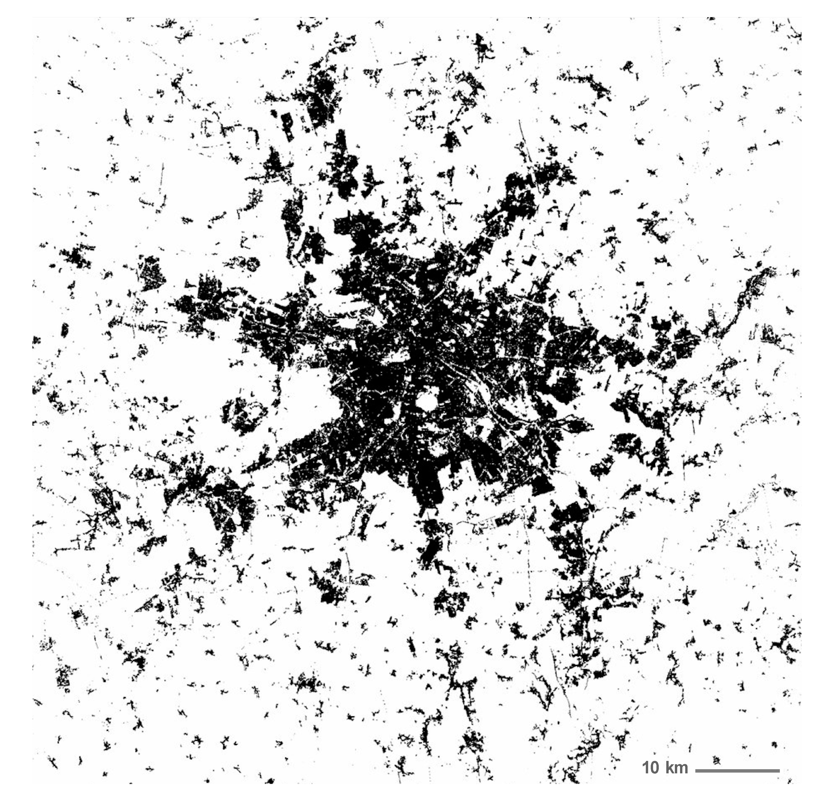
Table 1.
Urban climate change issues and major remote sensing tools available to address them, where AHI—Advanced Himawari Imager, ALOS—Advanced Land Observing Satellite, ASTER—Advanced Spaceborne Thermal Emission and Reflection Radiometer, CALIPSO—Cloud-Aerosol LiDAR and Infrared Pathfinder Satellite Observation, COSMO-SkyMed is Constellation of Small Satellites for Mediterranean basin Observation, DEM—digital elevation model, DMSP/OLS—Defense Meteorological Satellite Program’s Operational Linescan System, EROS—Earth Resources Observation Satellite, GDEM—Global Digital Elevation, MODIS is Moderate Resolution Imaging Spectroradiometer, OCO—Orbiting Carbon Observatory, OMI—Ozone Monitoring Instrument, SAR—Synthetic Aperture Radar, SRTM—Shuttle Radar Topography Mission, TANSO-FTS—Thermal and Near infrared Sensor for Carbon Observation—Fourier Transform Spectrometer, TES—Technology Experiment Satellite, VIIRS—Visible Infrared Imaging Radiometer Suite, VHR—Very High Resolution.
| Urban Climate Change Issues | Remote Sensing Capabilities | ||||||
|---|---|---|---|---|---|---|---|
| Urban Issue Linked to Climate Change | Quantity Needed | Quantity Obtainable or Available | Sensor | Spatial Resolution [m] | Temporal Resolution | Coverage | References |
| Urban population | Total population, density, and their change rates | Density, number, and type of dwelling units | Various Commercial VHR | 0.4–1 | on-demand/irregular | Irregular Global | Various vendors |
| Sentinel-1 | 10 | 6–12 days | Global | https://scihub.copernicus.eu/ | |||
| Sentinel-2 | 10–20 | 5–10 days | Global | https://scihub.copernicus.eu/ | |||
| TerraSAR-X Global Urban Footprint | 12 | 2011/2012 | Global | https://www.dlr.de/eoc/en/desktopdefault.aspx/tabid-9628/16557_read-40454/ | |||
| Landsat 8 | 15–30 | 16-day | Global | https://glovis.usgs.gov/ | |||
| Gaofen 1 and 6 | 16 | 2–4 days | Global | http://www.cnsageo.com/#/ | |||
| Urban extent and structure | Urban area and its composition Building height | Urban area Urban land uses Fractional vegetation cover | Various Commercial VHR | 0.4–1 | On-demand/irregular | On demand/Irregular | Various vendors |
| Sentinel-1 | 10 | 6–12 days | Global | https://scihub.copernicus.eu/ | |||
| Sentinel-2 | 10–20 | 5–10 days | Global | https://scihub.copernicus.eu/ | |||
| TerraSAR-X Global Urban Footprint | 12 | 2011/2012 | Global | https://www.dlr.de/eoc/en/desktopdefault.aspx/tabid-9628/16557_read-40454/ | |||
| Landsat 8 | 15–30 | 16-day | Global | https://glovis.usgs.gov/ | |||
| Gaofen 1 and 6 | 16 | 2–4 days | Global | http://www.cnsageo.com/#/ | |||
| MODIS Vegetation Indices | 250–1000 | 16-days | Global | https://lpdaac.usgs.gov/tools/earthdata-search/ | |||
| MODIS land cover | 500 | Yearly 2001–2017 | Global | https://lpdaac.usgs.gov/tools/earthdata-search/ | |||
| VIIRS | 750 | Monthly and yearly composites | Global | https://lpdaac.usgs.gov/tools/earthdata-search/ | |||
| Digital Urban Canopy Height | Various Commercial VHR, KOMPSAT-3 and other stereo images | 0.5–1 | 3 days | Global on demand | Various vendors | ||
| COSMO SkyMed | 1–100 | 4–16 days | Global | https://earth.esa.int/web/guest/-/cosmo-skymed-esa-archive | |||
| Sentinel-1 | 10–100 | 6–12 days | Global | https://scihub.copernicus.eu/ | |||
| ALOS World 3D | 5–30 | 2015 | Global | https://www.eorc.jaxa.jp/ALOS/en/aw3d30/data/index.htm | |||
| TanDEM-X DEM | 12–30–90 | 11 days | Global | https://geoservice.dlr.de/web/ | |||
| SRTM | 30 | 2000 | Global | http://srtm.csi.cgiar.org/srtmdata/ | |||
| ASTER GDEM V2 | 30 | Yearly 2000–2009 | Global | https://lpdaac.usgs.gov/ | |||
| Energy consumption | Consumption of energy Emissions of waste energy (heat) | RGB photography | International Space Station Astronaut photography | 5–200 | Irregular | Irregular | http://eol.jsc.nasa.gov/ |
| Multispectral Nighttime Light emissions | EROS-B | 0.7 | On demand | Tasked | https://apollomapping.com/eros-b-satellite-imagery | ||
| Jilin-1 (JL1-3B) | 0.9 | On demand | Tasked | https://www.cgsatellite.com/imagery/luminous-imagery/ | |||
| Jilin-1 (JL1-07/08) | 0.9 | On demand | Tasked | https://www.cgsatellite.com/imagery/luminous-imagery/ | |||
| Panchromatic Nighttime Light emissions | LuoJia1-01 | 130 | 15 days | Global | http://59.175.109.173:8888/app/login_en.html | ||
| VIIRS | 750 | Daily | Global | https://search.earthdata.nasa.gov/ | |||
| DMSP/OLS | 2700 | Yearly composite | Global | https://ngdc.noaa.gov/eog/dmsp/downloadV4composites.html | |||
| Thermal sensors | Landsat 8 | 100 | 16 days | Global | https://glovis.usgs.gov/ | ||
| ASTER | 90 | 16 days and on demand | Global | https://glovis.usgs.gov/ | |||
| VIIRS | 750 | Daily | Global | https://lpdaac.usgs.gov/tools/earthdata-search/ | |||
| MODIS | 1000 | Daily | Global | https://search.earthdata.nasa.gov/search | |||
| Sentinel-3 | 1000 | Daily | Global | https://scihub.copernicus.eu/ | |||
| Greenhouse gasses (CO2, CH4, N2O) | Emissions & concentrations | Concentrations of CO2 and CH4 in an air column | OCO-3 | 3500 | Irregular | 80 × 80 km area hotspots Snapshot Area Map (SAM) | https://search.earthdata.nasa.gov/search?q=OCO3_L2_Standard |
| Sentinel 5P | 7000 | Daily | Global | https://scihub.copernicus.eu/ | |||
| TanSAT | 1000 × 2000 | 16 days | Global | http://gsics.nsmc.org.cn/portal/en/satellite/TanSat.html | |||
| TANSO-FTS | 10500 | 3 days | Global | https://data2.gosat.nies.go.jp/index_en.html | |||
| TES | 5300 × 8500 | 2 days | Global | https://search.earthdata.nasa.gov/ | |||
| Other air pollutants | Emissions & concentrations of aerosols, ground level ozone, NOx, PM 2.5… | Concentrations of ozone, NO2, SO2 in an air column | Sentinel-5P | 7000 | Daily | Global | https://scihub.copernicus.eu/ |
| TES | 5300 × 8500 | 2 days | Global | https://search.earthdata.nasa.gov/ | |||
| OMI | 13000 × 24000 13000 × 13,000 zoom | Daily | Global | https://search.earthdata.nasa.gov/ | |||
| Aerosol Optical Depth | Sentinel-2 | 10 | 5, 10 days | Global | https://scihub.copernicus.eu/ | ||
| Landsat 8 | 30 | 16 day | Global | https://glovis.usgs.gov/ | |||
| VIIRS | 750 6000 | Daily | Global | https://data.nodc.noaa.gov/cgi-bin/iso?id=gov.noaa.ncdc:C01446 | |||
| CALIPSO | 5000 | Daily | Global | https://www-calipso.larc.nasa.gov/ | |||
| MODIS | 500, 1000, 3000, 10000 | 1–2 days | Global | https://search.earthdata.nasa.gov/ | |||
| Surface urban heat island and heat waves | Air temperature Land surface temperature Water temperature | Land Surface Temperature Water Surface temperature Sea Surface Temperature (SST) | ASTER | 90 | 16 days and on demand | Global | https://glovis.usgs.gov/ |
| Landsat 8 | 100 | 16 days | Global | https://glovis.usgs.gov/ | |||
| VIIRS | 750 | Daily | Global | https://lpdaac.usgs.gov/tools/earthdata-search/ | |||
| MODIS | 1000 | 4 times/day | Global | https://search.earthdata.nasa.gov/search | |||
| Sentinel-3 | 1000 | ~14 days | Global | https://scihub.copernicus.eu/ | |||
| AHI (SST only) | 2000 | Sub-daily | Global | https://coastwatch.noaa.gov/cw/satellite-data-products/sea-surface-temperature.html | |||
Publisher’s Note: MDPI stays neutral with regard to jurisdictional claims in published maps and institutional affiliations. |
© 2020 by the authors. Licensee MDPI, Basel, Switzerland. This article is an open access article distributed under the terms and conditions of the Creative Commons Attribution (CC BY) license (http://creativecommons.org/licenses/by/4.0/).
Share and Cite
MDPI and ACS Style
Milesi, C.; Churkina, G. Measuring and Monitoring Urban Impacts on Climate Change from Space. Remote Sens. 2020, 12, 3494. https://0-doi-org.brum.beds.ac.uk/10.3390/rs12213494
AMA Style
Milesi C, Churkina G. Measuring and Monitoring Urban Impacts on Climate Change from Space. Remote Sensing. 2020; 12(21):3494. https://0-doi-org.brum.beds.ac.uk/10.3390/rs12213494
Chicago/Turabian StyleMilesi, Cristina, and Galina Churkina. 2020. "Measuring and Monitoring Urban Impacts on Climate Change from Space" Remote Sensing 12, no. 21: 3494. https://0-doi-org.brum.beds.ac.uk/10.3390/rs12213494
Note that from the first issue of 2016, this journal uses article numbers instead of page numbers. See further details here.