1. Introduction
Land cover mapping provides information on the Earth’s surface characteristics. It is considered to be the most important variable in effective monitoring of natural and anthropogenic processes [
1], as it supports environmental and socio-economic decision-making [
2], and the implementation of various national and international programs and initiatives [
3,
4]. Continuous and reliable monitoring of land cover/use and land cover/use changes is necessary due to ongoing climate change, human population growth and the resulting agricultural expansion. It is also helpful in monitoring natural resources, ecosystem conditions, biodiversity as well as the estimation of losses due to natural and human-induced disasters. Consequently, it has been selected as one of the terrestrial essential climate variables used to analyse the state and characteristics of the Earth’s climate [
4,
5].
Earth Observation (EO) data are the most important source of information for land cover mapping due to the high spatial coverage, systematic monitoring and access to remote, inaccessible areas [
6,
7]. The first global land cover map was derived from EO data captured by the Advanced Very High Resolution Radiometer instrument flown on the National Oceanic and Atmospheric Administration’s satellites (NOAA-AVHRR) [
8]. Since then, imagery from many different satellites has been captured, and new image analysis techniques have been developed [
6,
9,
10,
11,
12,
13]. Land cover products have improved in terms of spatial extent (regional to global), level of detail (class range and composition, spatial resolution), update frequency, and the number of sub-products, among many other characteristics. Similarly, analysis techniques have improved, notably in terms of the level of automation, the sophistication of the method, and the amount of processed data. The present study, however, focuses on large-scale land cover mapping, and addresses research performed and tested on continental-to-global scale, with only exceptional cases of regional studies, highly relevant to the main subject.
The pioneering work of DeFries and Townshend [
8] was followed by numerous projects that developed global land cover products mainly based on data collected by coarse resolution instruments including, among others, NOAA-AVHRR, Satellite Pour l’Observation de la Terre Vegetation (SPOT Vegetation), Envisat MEdium Resolution Imaging Spectrometer (MERIS), and Moderate Resolution Imaging Spectroradiometer (MODIS) [
14,
15,
16,
17,
18]. Although there were numerous applications of these products, they were characterised by significant inconsistencies and a low level of details [
6,
7,
19]. At the same time, there was a high demand within the user community for large-area land cover datasets with higher spatial resolution, produced at higher temporal frequency [
6,
7]. The cost of developing such a product was, however, prohibitive until the Landsat archive was made available to all users, free of charge in 2008. This was followed by improvements in computing performance, and numerous global datasets with 30 m spatial resolution were produced including both single- and multi-class data [
7,
20,
21,
22,
23,
24]. Although Landsat data increased the spatial resolution and level of detail of newly-developed products, similar improvements in thematic accuracy have not been seen in all cases, compared to lower-resolution datasets. Currently, even higher resolution products are feasible due to the regular collection of EO data by Sentinel-2 and -1 satellites, and its provision under free and open access policies.
At the present time, there are several programs that manage the production of regularly-updated regional or continental databases [
3,
25,
26,
27]. Such products make it possible to directly monitor changes that appear between consecutive database releases, while maintaining the same class definitions. For example, the CORINE and Cover (CLC) database [
25] is the flagship European database, with 44 land cover/use classes. The first version was produced for the reference year 1990 and have seen four updates covering the period between 1990 and 2018. However, as the workflow remains heavily dependent on manual work by dozens of national teams, the update frequency remains low. Furthermore, the CLC’s minimum mapping unit (MMU) of 25 ha is another limitation to its usefulness, as many applications require a higher level of detail. Although other products, such as for instance, High Resolution Layers (HRLs) [
26] and the products of the North American Land Change Monitoring System [
3], are available at much higher spatial resolution (20 m and 30 m, respectively), the update frequency is low (i.e., 3–5 years). Additionally, HRLs only cover five land cover types (impervious areas, forests, grasslands, wetness and water, and small woody features), which limits the thematic information they provide. Considerable effort has also been made to produce the United State National Land Cover Database (NLCD), including updates that cover a time period between 1990 and 2016, that is similar to CLC data [
28,
29]. However, it should be noted that, although a comprehensive set of products is provided, with this 30 m spatial resolution database covering the conterminous Unites State, its production is not fully-automated and requires access to extensive sets of reference data.
The performance of most classification techniques, especially supervised ones, relies on the quality and quantity of training samples [
30]. The collection of a sample suitable for large-scale mapping is often seen as a bottleneck, and may require a tremendous amount of manual work [
31,
32]. For example, Gong et al. [
20,
33] and Li et al. [
34] produced large-scale, high resolution land cover databases, however they required the enormous and usually cost-intensive manual visual image interpretation that seriously hampers repetitive and regular (e.g., annual) map production or their update [
1].
There is an increasing number of applications that require high spatial resolution products and more frequent updates [
3,
32,
33]. Given the currently available satellite missions, the annual production of a high spatial resolution land cover/use database is feasible, but requires a very high level of automation. Therefore, there is a clear need for an operational method that can be applied at local to global scales that will enable efficient, reliable, and automated processing of high resolution EO data.
One automated way to collect training data for large-scale mapping is to extract samples from existing land cover/use databases. There have already been several promising attempts to test such an approach [
1,
3,
32,
35,
36]. In most cases, however, EO imagery has been classified at similar or lower spatial resolution than the reference source. High spatial resolution mapping can only be achieved by using local databases, which are necessarily spatially-limited and insufficient for large-scale continental or global mapping. It therefore seems useful to test the potential effectiveness of training samples derived from databases that have lower spatial resolution than the satellite data being classified. Such an approach has not been widely evaluated in large-scale land cover mapping.
This challenge was addressed within the Sentinel-2 Global Land Cover (S2GLC) project [
37], funded by the European Space Agency. The project ran from 2016 to 2019 and aimed to develop a land cover/use classification methodology ready for implementation on a global scale. The goal was to develop a method based on satellite imagery acquired by Sentinel-2 sensors, and deliver a product with 10-m spatial resolution. Extensive analyses were carried out in test areas located in various parts of the world, including large regions of Africa, Asia, Europe, and South America. Among the various approaches that have been tested, a supervised method based on training data extracted from existing low-resolution databases was selected as the most appropriate, as it enables global land cover mapping without manual the collection of training data [
38]. This paper presents the results of the operational implementation of the developed approach to a wide area of the European continent.
The overall goal of this study was to develop a highly-automated and ready for operational use, land cover/use classification methodology that could be applied on a large-scale, from regional to global. The more detailed objectives were:
To develop a method to generate a unified, reference training dataset from existing land cover databases.
To develop an automated classification workflow based on multi-temporal Sentinel-2 imagery, resulting in a final product with high spatial resolution (10-m) and thematic accuracy.
To optimise data processing by using the Data and Information Access Services (DIAS) cloud-based computing environment.
A key assumption was that information contained in land cover databases used as the reference, and source satellite images were sufficient to produce reliable land cover/use mapping on a large scale. We also assumed that Sentinel-2 data with spatial resolution up to 10 m would enable a detailed analysis of heterogeneous areas, and provide more accurate estimates of class coverage [
33].
2. Materials and Methods
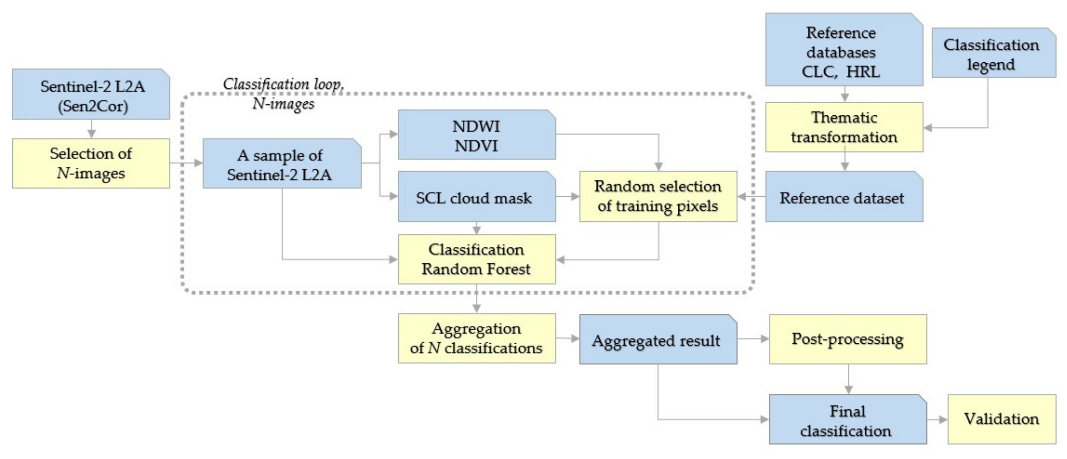
Figure 1 presents the overall structure of our automated land cover/use classification procedure. In general, it follows a supervised remote sensing methodology. The workflow starts with the selection of a set of Sentinel-2 images from a time series covering the whole of the year 2017. Then, training samples are selected for classification using a random forest machine learning algorithm. Next, the results of the classification of individual images are aggregated, and post-processed. Finally, the results are validated. All calculations and data processing was carried out on CREODIAS [
39], one of five cloud-based DIAS computing platforms deployed by the European Commission [
40].
The following sections provide details of each step in the procedure. It should be noted that, with the exception of the last step, all data analyses and processing was performed on a tile-by-tile basis.
2.1. Study Area
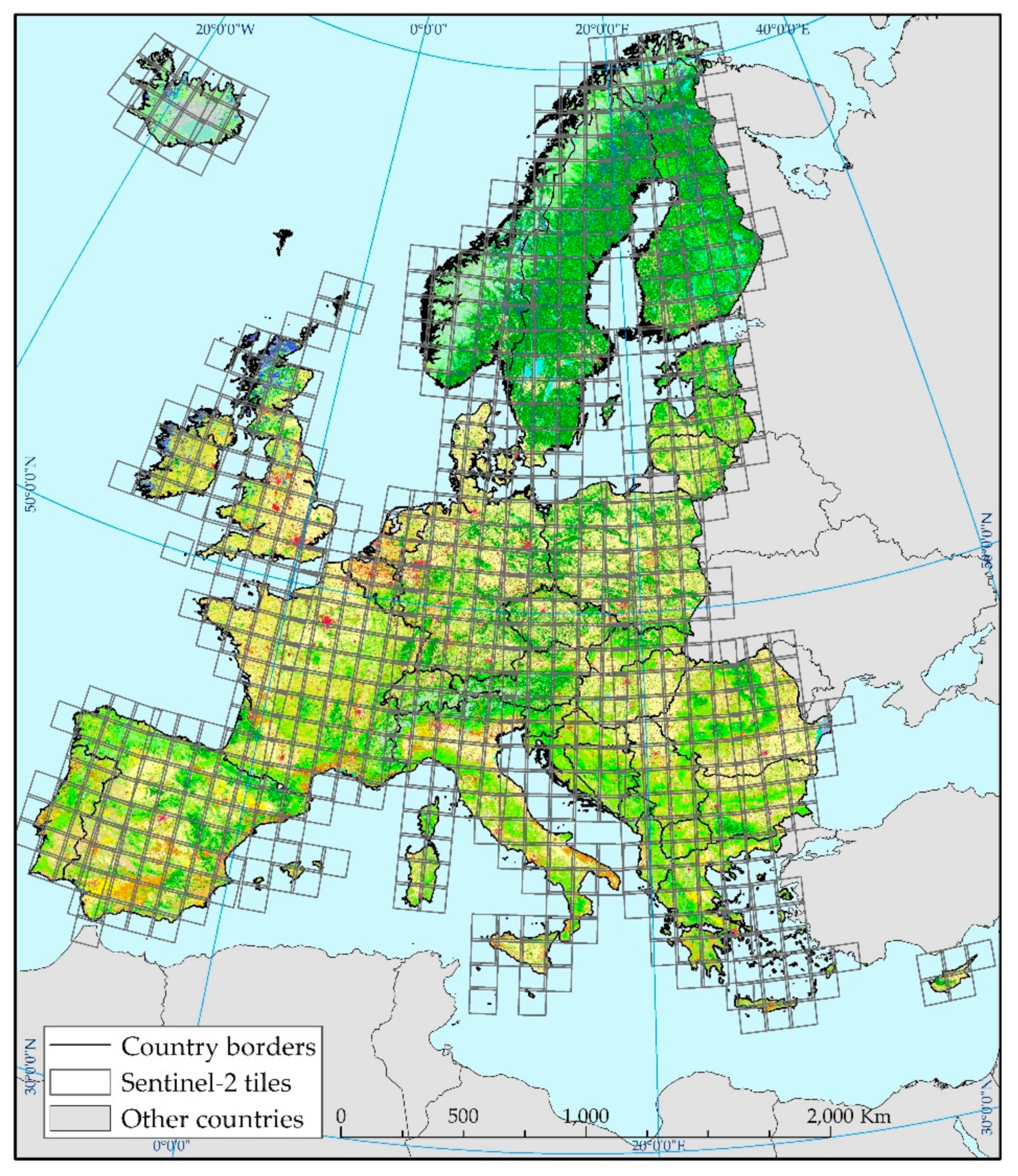
The main study area covers 27 European Union Member States together with Liechtenstein, Norway, Switzerland, the United Kingdom, the Western Balkans and Iceland. It also encompasses the Mediterranean islands (the Greek Islands, Cyprus, Malta, Sicily, Sardinia, Corsica, the Balearic Islands), and islands surrounding the United Kingdom and Ireland (
Figure 2). This geographical zone is similar to the CLC database [
25], with the exception of Turkey (
Figure 3). The analysed area corresponds to 791 standard Sentinel-2 tiles (granules) [
41]. The resulting land cover/use map covers 34 countries with climates that vary from dry and hot (the Mediterranean, southern Europe) to cold and boreal (the far north).
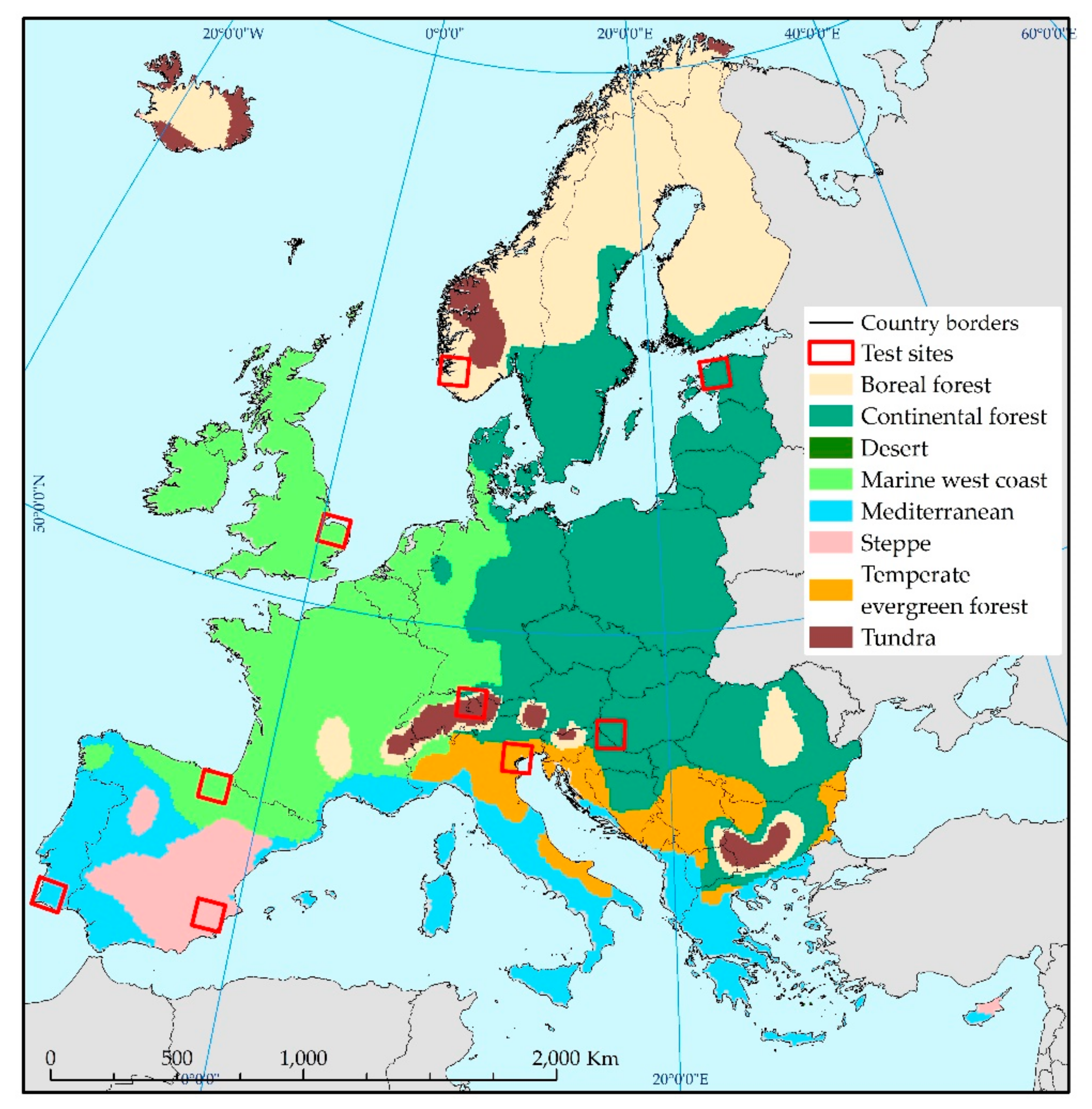
The initial, development phase that preceded classification of the whole study area aimed to design and test individual parts of the classification methodology. These tests were performed on selected sites representing different European climatic regions. The division into climatic classes was based on the Köppen–Geiger climate classification system, updated by Peel et al. [
42], and the stratification method proposed by Olofsson et al. [
43]. Consequently, the area was divided into seven regions: boreal forest, continental forest, marine west coast, Mediterranean, steppe, temperate evergreen forest, and tundra (
Figure 3). A test site was selected for each region, while the two biggest regions, i.e., continental forest and marine west coast, were represented by two sites. Each test site corresponds to a single Sentinel-2 tile, covering an area of 110 × 110 km.
2.2. Input Data
2.2.1. Sentinel-2 Imagery
We used multi-temporal Sentinel-2 data originating from the Copernicus program. These data are particularly suited to operational land cover mapping at regional to global scale. Sentinel-2 sensors provide 13 spectral band imagery, with spatial resolution ranging from 10 m to 60 m, covering visible, near-infrared and short-infrared parts of the electromagnetic spectrum [
41]. Additionally, Sentinel-2 data are the only free of charge, spaceborne imagery produced at such high spatial resolution. We selected 2017, as this was the first year in which both Sentinel-2 satellites (Sentinel-2A and Sentinel-2B) operated. Sentinel-2A has been collecting data since the second half of 2015, while Sentinel-2B started operating in the middle of 2017. The operation of both sensors increased the revisit period to five days, and improved the availability of cloud-free data.
In order to avoid classifying all available Sentinel-2 images, and to reduce computation requirements, we developed a data selection strategy. The aim was to select, for every Sentinel-2 tile in the study area, the two, least-cloudy images for each month in the growing season (April to October) and one for each of the remaining months (January–March and November–December). Specifically, over 50% of the image area had to be cloud-free (cloud, cloud shadows and areas with no data making up the remainder). Therefore, the method assumes the use of 19 images per tile, in ideal conditions. If, in a given month, no image met the criteria, an image from another month with the closest acquisition date was used. These rules were modified for mountainous tiles, tiles with diverse relief, and those with steep, long slopes. The deep shadows in such areas, for images acquired between October and March, led to them being excluded from the analysis. In a few cases, data selection criteria were not met, and less than 19 images were classified.
Sentinel-2′s L2A products were accessed from the CREODIAS platform, after atmospheric correction performed with the Sen2Cor processor [
41], and representing Bottom-Of-Atmosphere surface reflectance values. Data analyses were only performed on 10 m and 20 m spatial resolution bands, with the latter resampled to 10 m resolution by the nearest neighbour method. Spectral bands with 60 m spatial resolution were excluded, due to their limited usefulness for land surface analyses [
44]. The L2A product also includes a scene classification (SCL) map, which provides information on, among other things, the extent of different types of cloud and cloud shadow [
41]. The SCL map was used during image processing and classification to mask image pixels and reference data covered by cloud and cloud shadow.
2.2.2. Classification System
Drawing upon the available reference data sources, that include the CLC and HRLs (more details provided in
Section 2.2.3), we developed a classification legend composed of 13 classes, and an additional class representing surfaces permanently covered by cloud (
Table 1). The overall goal was to develop relatively general, common classes that would make it possible to automate the selection of reference samples and data classification. A second requirement was that the selected classes should be highly homogenous and represent relatively similar characteristics across Europe. Therefore, most of the selected classes represent the physical characteristics of surface cover (land cover), and not how the land is used (land use). Only two classes (artificial surfaces and cultivated areas) can represent different land cover types, as they are managed and used for various purposes. Thus, for simplicity, we use the term land cover in the remaining part of the manuscript for all the mapped classes.
2.2.3. Training Data Sources
The output of a supervised classification relies on the quality and quantity of training samples. Therefore, their appropriate preparation is a crucial step in the workflow. However, the collection of the qualitatively homogenous training dataset on a continental or global scale is a very demanding task [
34,
45]. Field surveys are infeasible due to the high cost, the required time and workload. Visual interpretation of high resolution EO data is also time-consuming and requires access to a huge set of aerial photography, satellite imagery, or maps. Therefore, the optimal solution is to use existing land cover databases as the data source. Our method drew upon two databases (the CLC and HRLs) to provide complementary information on land cover across the whole study area.
The CLC database is one of the most popular and widely used pan-European land cover databases [
25]. Composed of 44 classes, it provides rich and harmonised information on land cover, land use, and changes that occurred between updates, starting from 1990. Produced by national teams, it is integrated and coordinated at the European level by the European Environment Agency. CLC is mainly produced by visual interpretation of EO data (e.g., Landsat, SPOT, LISS III and, more recently, Sentinel) with a limited level of automation. The nominal scale is 1:100 000 with a MMU of 25 ha for a single areal object, and a minimum width of 100 m for linear objects. The 2012 version of the CLC database was used to produce the training dataset, as it was the most up-to-date version available at the time of our data processing.
HRLs were developed under the Copernicus program. These databases represent information on several land cover types. Each layer shows the distribution of an individual class, together with its characteristics. HRLs are available at 20 m or 100 m resolution and, therefore, outperform CLC in most cases, notably in terms of the detailed outline of certain objects, and more homogenous classes. The method used to produce HRLs combines automated and interactive rule-based classification of EO images, for both optical and radar data [
26]. In this study, we used 20 m resolution HRL imperviousness, grassland, and forest layers products from the year 2015.
HRL Imperviousness represents sealed areas as a degree of imperviousness, ranging from 0–100% [
46], reflecting built-up areas and other artificial cover. The database was produced using an automated procedure, based on calibrated normalized difference vegetation index (NDVI) values, with overall accuracy (OA) estimated to be above 90% [
47]. HRL grassland represents the spatial distribution of grassland and non-grassland areas. This grassy and non-woody vegetation product encompasses natural grassy vegetation, semi-natural grasslands, and managed grasslands, but excludes crop areas [
48]. The OA of the grassland layer used in this study is estimated to be approximately 85% [
48,
49]. HRL Forest consists of the following products: tree cover density (TCD) representing the per-pixel crown coverage in the range 0–100%; and dominant leaf type (DLT) which provides information on the dominant leaf type: broadleaved or coniferous [
50]. The TCD product is characterized by high user’s and producer’s accuracy of above 85% ([
51] p. 52), with accuracies of DLT product being in the range of 70–88% for broadleaved and coniferous leaf types ([
51] p. 59).
Finally, the Advanced Spaceborne Thermal Emission and Reflection Radiometer (ASTER) Global Digital Elevation Model (GDEM) version 2 was used to correct the land cover map in the post-processing phase. ASTER GDEM is a global elevation dataset that is produced jointly by the Japanese Ministry of Economy, Trade, and Industry, and the United States National Aeronautics and Space Administration. GDEM horizontal resolution is 2.4 arc-seconds (72 m), with 12.6 m standard deviation in elevation error [
52].
2.2.4. Training Data Preparation
Both CLC and HRL datasets were respectively re-projected, rasterised and resampled to fit into a pixel of Sentinel-2 data. Reference databases were subdivided into parts corresponding to individual Sentinel-2 tiles. Tiles were stored using the Universal Transverse Mercator projection, the original projection of Sentinel-2 product.
The strategy to select training samples from available databases was investigated and developed in the mentioned developing phase. The performed tests focused on the use of different combinations of reference datasets and spectral indices, and helped to design rules for the selection of samples for each land cover class. The aim was to develop rules that were transparent, easy to apply, able to be fully automated, and that did not require the application of any other data sources beyond CLC, HRLs and Sentinel-2. Selection of optimal rules for particular classes resulted from analyses performed within the predefined test sites. A detailed summary of the composition of the training dataset and filtration rules for all land cover classes is presented in
Table 2.
In most cases (cultivated areas, vineyards, sclerophyllous vegetation, marshes, peatbogs, natural material surfaces, permanent snow) training datasets were taken from the corresponding CLC classes (
Table 2). They were, however, filtered using the Normalized Difference Water Index (NDWI), HRL Imperviousness, HRL TCD and HRL Grassland, and empirically-estimated thresholds (
Table 2). This step was intended to reduce mislabelling resulting from the generalisation of the CLC dataset, and its MMU. Additionally, the natural material surfaces class was filtered with the NDVI, as there should be no vegetation in this class. Samples for artificial surfaces and herbaceous vegetation were taken from HRL Imperviousness and HRL Grassland layers, respectively, and were also filtered using the NDWI, and the other HRL Imperviousness, HRL TCD and HRL Grassland datasets.
For broadleaf and coniferous tree cover classes, training data were prepared based on the spatial intersection of the HRL DLT dataset and the CLC classes broadleaved forest (3.1.1.) and coniferous forest (3.1.2.), respectively. These classes were also filtered using the NDWI, HRL Imperviousness and HRL Grassland data. The moors and heathland class were similarly filtered using the NDWI, HRL imperviousness, and HRL TCD.
Finally, frequent changes in the extent of water surfaces meant that training data for the water bodies class required a different approach. They were derived by combining NDWI and CLC water-related classes. The water mask resulting from NDWI thresholding (> 0.2) was subdivided into inland waters (5.1.1., 5.1.2.) and marine waters (5.2.1., 5.2.2., 5.2.3.) with the appropriate CLC classes. In tiles where both sub-classes occurred, training samples for the water bodies class were selected equally from both. This approach ensured the uniform representation of all types of water surfaces in the classification model [
45]. Training samples for the water bodies class were also filtered with an NDVI threshold of <0.25 to exclude pixels with a vegetation component.
It is important to note that filtration with the NDVI and the NDWI was performed separately for the classification of each Sentinel-2 image. This approach helps to clean artefacts resulting from the low resolution of reference databases, or due to changing environmental conditions (e.g., floods). The main purpose of the filtration rules was to filter out false positives in a given land cover class, although it should be noted that they may also have excluded some true positives. Nevertheless, in most cases, dozens of thousands of samples could be selected for each class, for each tile. The size of this dataset meant that the required subset of samples could be selected for multiple classifications.
2.3. Classificaiton Procedure
2.3.1. Classification Features and Algorithm
The core element in the procedure is the pixel-based classification of Sentinel-2 images. Images in every tile were independently analysed. The random forest classifier was applied. This ensemble-based algorithm generates numerous decision trees from a randomly-selected subset of both training samples and classification features [
53]. The characteristics of the random forest classifier makes it more resistant to overfitting, and erroneous training samples than other machine learning algorithms [
54]. The final decision is based on classification results from all decision trees, using majority voting. The two main parameters of random forest are the number of trees to be generated and the number of features selected for each split in the tree. We used a relatively small set of trees (50) to limit the calculation time, as increasing the number of trees has only a minor influence on the final classification result [
55,
56]. The second parameter was set to the square root of the number of input features, which also helped to limit the computational complexity of the classifier [
57].
For every tile, each Sentinel-2 image was classified separately at pixel level, with a new set of training samples selected randomly from the prepared dataset (
Section 2.2.4.). The number of training samples was set to 1000 for every class, with a minimum of 50 (for very cloudy images). Pixels representing cloud and cloud shadow were masked using information from the SCL map.
It is common practice to use, besides the spectral bands of satellite imagery, other explanatory variables (classification features), such as spectral indices derived from the analysed images [
34,
58,
59,
60,
61]. Therefore, to enhance recognition of land cover classes, we fed the classifier with similar features. However, instead of calculating predefined, commonly-used indices such as NDVI, we calculated all possible combinations of Sentinel-2 spectral bands following Equation (1), namely the normalised difference between two spectral bands:
where BandX and BandY are any two bands of a satellite image. A total of 100 features were available for classification for every analysed Sentinel-2 image.
2.3.2. Aggregation
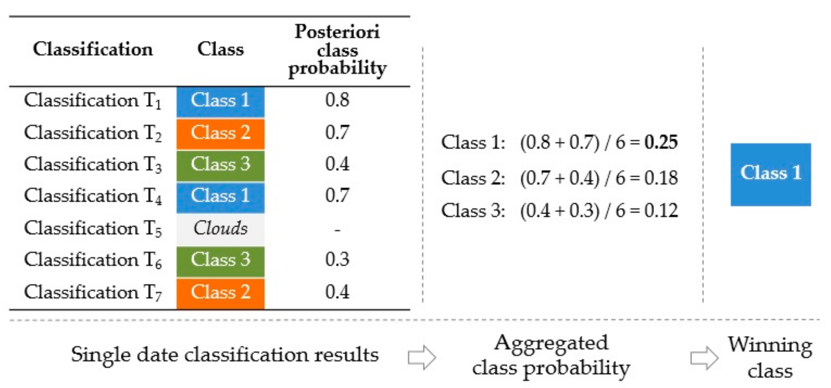
After classification of all Sentinel-2 data, the results from individual images for every tile were combined into a single output. This procedure, called aggregation, was developed as an alternative to the analysis of multi-temporal data [
62]. The method is based on two sets of input data, both resulting from the application of the random forest classifier. The first is the classification result, in the form of a thematic land cover map. The second, often called the posteriori class probability [
11,
63], is a raster image that presents information on the number of trees voting for the final class found in the ensemble, for each classified pixel, divided by the total number of trees [
3]. In the aggregation process, posteriori probability values are summed, for each land cover class found in the investigated pixel, from all images of a time series. Then, the sum is divided by the number of all valid occurrences (not cloudy) in a time series, regardless of the class label. The method assumes that individual classifications are not weighted by acquisition date, cloud coverage or thematic accuracy. The only weighting factor is the posteriori probability, which is applied to each pixel individually, as explained above.
Figure 4 presents an example of the aggregation process for a single pixel.
2.3.3. Post-Processing
Post-processing aimed to refine the classification result, by reducing post-classification errors. It was applied to the map resulting from the aggregation process. Classification errors are typically due to spectral similarities between classes, or spectral values that are influenced by terrain characteristics such as slope, altitude or sun illumination [
22]. A commonly-used method is to replace noisy, isolated pixels (the salt-and-pepper effect) using median filters [
11], resulting in a smoothed thematic map. However, all small objects represented by single pixels, including those that have been correctly classified, are removed. Our procedure only modifies pixels with a relatively low posteriori class probability obtained from the random forest classifier, and modified during aggregation. In addition, for each given pixel, information about its surrounding pixels is analysed, along with slope and altitude characteristics derived from the digital elevation model.
All five post-processing steps concern the artificial surfaces class. Built-up areas are characterised by a wide range of spectral values, and are spectrally similar to other land cover types such as bare soil, rock, and other bright surfaces. Consequently, the class is frequently overestimated, and our refinement aims to reduce misclassification. The following steps were designed to be performed in sequence, while parameter and threshold values were derived during the development phase of the study:
Pixels in the class artificial surfaces with posteriori probability values below 0.35 are reclassified as belonging to the neighbouring class that they have the longest border with.
Pixels located on the edges of water surfaces (rivers, lakes, seas) are reclassified as water bodies if they are initially classified as artificial surfaces with a posteriori probability value below 0.48, and if the adjacent water body covers over 5 ha.
Pixels in the artificial surfaces class are reclassified as natural material surfaces if the posteriori probability value is below 0.48, and if they are completely surrounded by an area, classified as natural material surfaces larger than 1 ha.
Pixels classified as artificial surfaces, located in high mountain regions, above a certain altitude or on steep slopes are reclassified as the next class given by ranking of posteriori probability values. Thresholds are adjusted to fit the characteristics of different mountainous areas in Europe. The rule was applied to 171 mountainous tiles.
The last step was related to the erroneous cloud mask originating from the Sen2Cor processor [
64]. Some areas with high spectral reflection values, such as built-up areas, are misclassified in the cloud mask as cloud. Consequently, in some cases, all cities, especially in the south of Europe, are permanently masked out. To minimise this problem, for every tile, the least-cloudy image from the predefined time series was selected and classified without applying the cloud mask. In this way, incorrectly masked-out pixels from the result of the aggregation were replaced with the result of the classification of the least-cloudy image.
2.4. Validation of the Land Cover Map
We validated the thematic accuracy of the land cover map product, consisting of 13 classes (
Table 1) and cloud, which was the result of the post-processing of the aggregated time series classifications. To ensure that the assessment was unbiased and reliable, a fully-independent reference dataset was created.
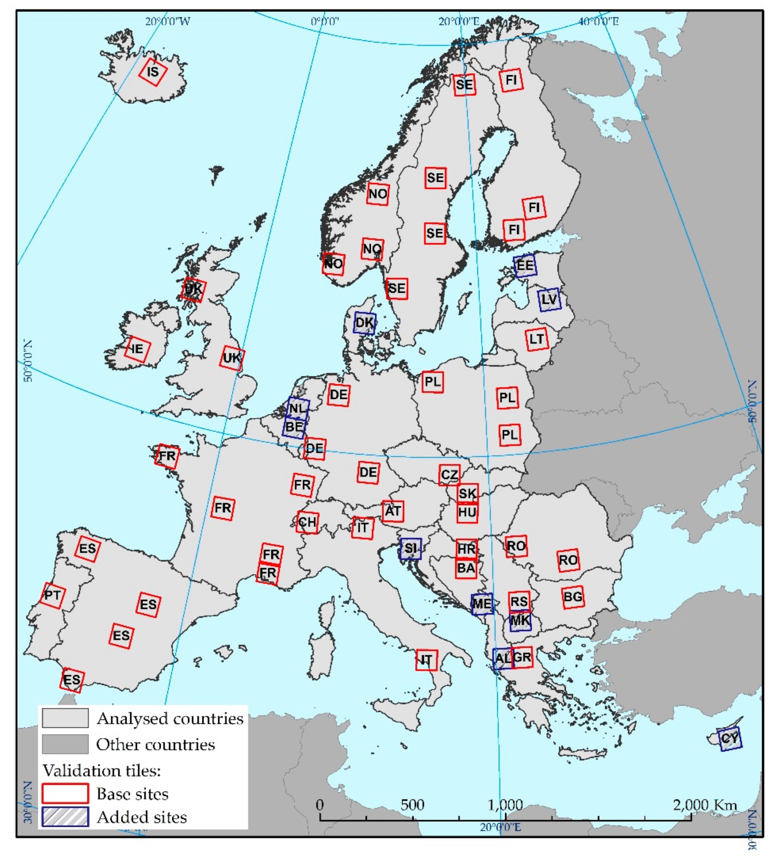
The selected validation sites were distributed by stratified random sampling with proportional allocation over Europe, with country borders representing stratum in the dataset. The sampling strategy was based on a single Sentinel-2 tile covered by at least 75% land. The accuracy assessment was performed for approximately 10% of all Sentinel-2 tiles in each country, except for Andorra, the Vatican, San Marino, and Lichtenstein (
Figure 5). These sites were named “base sites”. Luxemburg was included in one of three sites selected for Germany (
Figure 5). For some countries, the selected Sentinel-2 tiles reached near-zero values. In these cases, to assure the accuracy assessment on a country level, it had been decided to randomly select a single tile, named “added sites” (
Figure 5). Sites located at national borders were merged with sites selected for the neighbouring country, and are represented in the summary as validation sites for the two countries. This was the case for Albania and Greece, and Croatia and Slovenia.
Table 3 presents a summary of validation sites and sample selection.
The stratification of validation samples was based on CLC reference data. We selected the appropriate land cover class using our legend (
Table 1). An additional class was created by merging all the remaining CLC classes. Samples were selected randomly from all classes within the strata, as a function of the proportion of a given class within a specific Sentinel-2 tile, and were submitted for verification without the predefined land cover class given in the attribute table. Following the assumption of the selected samples clear identification in respect to the assessed outcome and reference data, the number of selected samples was increased from pre-estimated 800–1000 per tile. This approach was driven by the fact that some samples needed to be eliminated due to their location on a border between land cover classes or, in specific cases, the inability to identify a class.
The following conditions were applied to the stratification process:
Land cover classes covering less than 0.95% of a tile were excluded.
For land cover classes covering between 0.95–2% of a tile, a minimum of 20 validation samples was set.
For artificial surfaces and natural material surfaces classes, a default minimum of 20 validation samples was set, even if they covered less than 0.95% of a tile.
This strategy resulted in a set of 55,000 initial samples for the 55 validation sites.
Verification of the initial sample dataset was based on reference data. The latter had to meet rigorous criteria, in order to compensate for missing ‘ground truth’ found in in-situ surveys. The main objective was to verify samples against real-world conditions carried out as virtual truthing with EO data. Therefore, the applicable EO data had to have the same or preferably higher spatial resolution, and represent the same time span as the data used to produce the land cover map. Planet Scope imagery, in combination with Sentinel-2 was chosen, representing a similar time range. This latter criterion is necessary to ensure the correct analysis of samples representing classes with seasonal changes, where multi-temporal analysis is necessary.
Verification took the form of a stable, manual, but efficient workflow. The area was divided into zones representing different climate regions, with each zone coordinated by an expert in the area. The process resulted in a very rich set of 51,926 samples that could be used to validate the thematic maps. The minimum number of 800 samples was met for all sites. The final stage was to compare the reference data with the results of the automatic classification. We developed metrics that indicated thematic accuracy in terms of the effectiveness and reliability of the information content group. Using validation samples, confusion matrices were calculated for each country, and for the entire study area. In addition to the overall classification accuracy, the confusion matrix presents individual accuracies for each land cover category, along with both user’s accuracy (commission errors) and producer’s accuracy (omission errors). Finally, the F1 score was calculated to indicate the balance between commission and omission errors.
3. Results
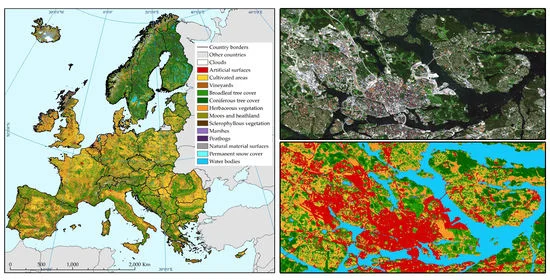
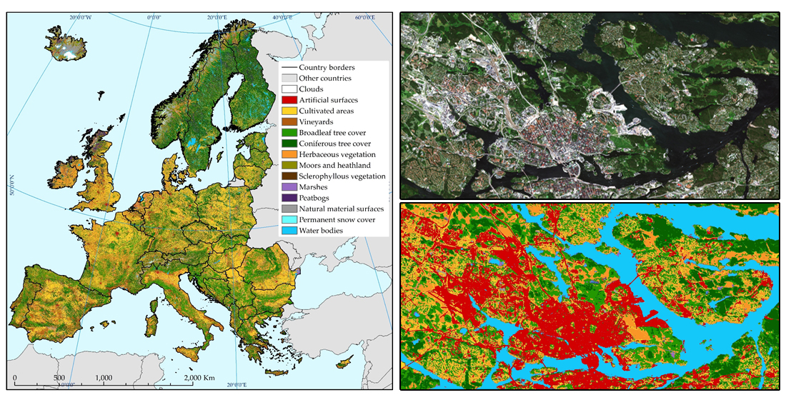
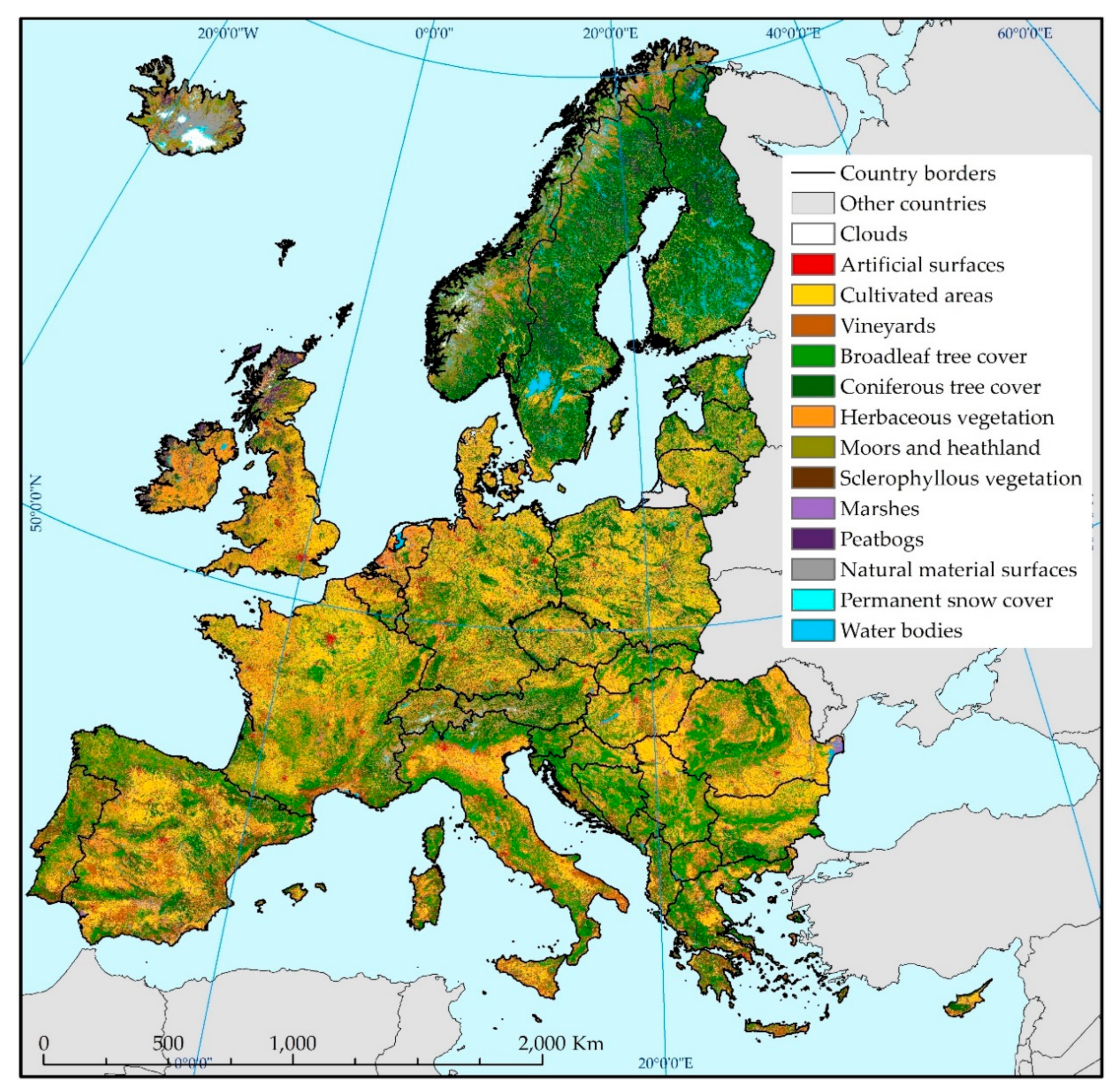
Figure 6 illustrates the results of the land cover classification performed with our methodology, for the year 2017, at a spatial resolution of 10 m. The map is composed of 791 separately classified Sentinel-2 tiles, trimmed to take account of coastlines. Most of the sea area in the water bodies class, along with areas in external countries, was excluded. This map can be downloaded from the S2GLC project website and the CREODIAS platform [
37]. Our classification found that the most widespread classes were cultivated areas (nearly 20% of the study area), broadleaf tree cover (19%), herbaceous vegetation (19%) and coniferous tree cover (over 16%). The remaining nine classes sum up to only 25% of the study area.
Table 4 presents the confusion matrix; accuracy measures are derived from samples for all validation sites. On a continental level, our classification achieved 86.1% OA, with a kappa coefficient of 0.83, and a weighted average F1 score of 0.86. At the land cover class level, water bodies and coniferous tree cover were identified most accurately (F1 score 0.96), followed by broadleaf tree cover (0.95) and cultivated areas (0.91). Accuracy was lowest for permanent snow (0.16), sclerophyllous vegetation (0.30) and marshes (0.30).
The F1 score was above 0.91 for most of the classes with the widest coverage. The exception was herbaceous vegetation, with a score of 0.77. Here, grassy vegetation was confused with cultivated areas, and moors and heathland (
Table 4). Among the less-frequent classes, the F1 score was highest for water bodies, followed by artificial surfaces (0.80) and natural material surfaces (0.70). The two last classes were also mixed often with each other. Peatbogs (F1 score 0.66) were often confused with moors and heathlands (F1 score 0.45), which, in turn, were frequently misclassified as herbaceous vegetation. Accuracy was moderate (F1 score 0.60) for vineyards, despite a high producer’s accuracy (89%). This result was due to their misclassification as cultivated areas.
At the country level, OA values range from 67% to over 95% for all 32 countries (or pairs of countries) (
Table 5). For all countries, average OA is high (86.5%) and the average kappa coefficient is 0.82.
Table 5 shows that OA for 12 of the 32 countries exceeded a high value of 90%, while 14 countries fall in the range 80–90%. For the other five countries, OA was in the range 70–80%, and was below 70% for only one country. OA scores were highest for the Germany/ Luxemburg pair (95.8%), Slovakia (95.4%) and Ireland (95.0%), and scores were lowest for Portugal (67.0%). From a climatic perspective, accuracy was relatively evenly distributed, although values were slightly lower for Mediterranean countries (
Table 5).
The post-processing procedure only increased OA by 0.3% (from 85.8% to 86.1%) on a continental scale. However, a greater improvement was observed for the artificial surfaces class. Although producer’s accuracy decreased by 3% (to 85.1%), user’s accuracy increased by 13%, and the F1 score by 7%. Accuracies of most of the remaining classes did not change considerably. The extent of areas affected by post-processing was a function of the local land cover type, and reached a maximum of 5.7% for one tile. On a continental scale, 1.2% of the entire study area (60 633 km2) was modified by post-processing.
4. Discussion
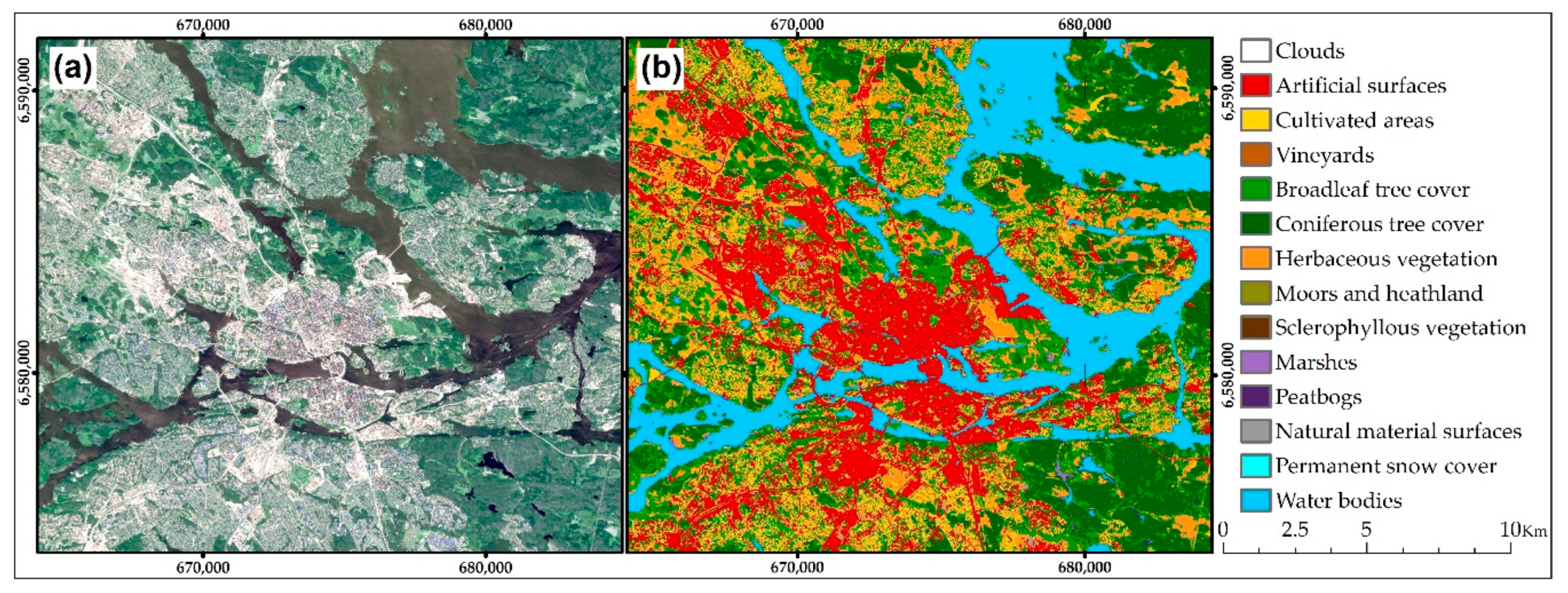
This study aimed to develop a complete, ready for operational use automated land cover classification workflow based on multi-temporal Sentinel-2 imagery. The proposed procedure meets all predefined objectives. It demonstrates that it is possible to fully automate all of the steps required to process large datasets, from training data preparation, access to Sentinel-2 imagery, to data classification and post-processing. The high automation of the method enables straightforward processing of new training and EO data, and frequent and repetitive large-scale production of land cover maps. Furthermore, the 10-m spatial resolution ensures a very high level of detail of the landscape (
Figure 7).
The operability of our classification system is enhanced by the application of the CREODIAS computing environment. On the one hand, CREODIAS supplies the system with Sentinel-2 data and, on the other hand, enables the efficient analysis of huge datasets that remarkably streamlines overall data processing.
Our analyses of Sentinel-2 data uses a cloud mask originating from the Sen2Core processor, regardless of its drawback related to the misinterpretation of high-reflectance areas [
64,
65]. However, application of ready-to-use datasets, available from the Copernicus Scientific Hub or CREODIAS, allowed avoiding additional testing and the implementation of third-party algorithms and processing tools. This strategy increases the operational usefulness of our method, which relies entirely on open-source components.
4.1. Classificaiton Accuracy
OA of 86.1% is very high for an automated method, and a promising indication for the future. Classification accuracy for individual land cover classes varies, with the most accurate results obtained for the most highly-represented classes of cultivated areas, broadleaf tree cover, coniferous tree cover, herbaceous vegetation and water bodies [
33]. Almost all producer’s and user’s accuracies of these classes were well above 80%, and often exceeded 90% for both or one of them (
Table 4). Additionally, good results were obtained for the artificial surfaces class, despite the much lower spatial coverage. It was very well recognised by the classifier (omission errors < 15%) and is characterised by a relatively low level of commission error (approx. 25%).
Other classes, with relatively low spatial coverage, were less-well classified. Examples include shrubland classes (moors and heathland, sclerophyllous vegetation) and wetland classes (marshes and peatbogs) (
Table 4). These groups appear to be very difficult to map accurately. However, our results are consistent with other studies, which find that accuracy is lower for wetlands and shrublands than other vegetation types [
20,
33,
58,
59,
66]. Therefore, the poor recognition of these classes in our study is neither related to the high level of automation, nor to the large scale of the mapping. Instead, it can be attributed to the spectral similarity of these classes both with other vegetation classes, and between each other [
67].
The very low accuracy for the permanent snow cover class may be explained by outdated CLC reference training data, and shrinking permanent snow cover and glaciers in the Alps, Scandinavia, and Iceland [
68,
69]. Another reason is that the high reflectance of this class is similar to the natural material surfaces class. This similarity, and the natural coexistence of these classes, increases misclassification. This class was also represented by the fewest validation samples, which may have further reduced accuracy.
Undoubtedly, further research is needed to improve the quality of recognition of all of the poorly-classified classes in our study. The analysis of our classification results suggests that the legend could be modified to combine selected classes, based on their thematic and spectral similarity. The results of our study suggest that vineyards could be combined with cultivated areas, moors and heathland could be combined with herbaceous vegetation, and marshes could be combined with peatbogs. These combinations would increase OA from 86.1% to 89.0%. A classification based on 10 rather than 13 classes would provide improved and more homogeneous classification results for nearly all classes (except permanent snow and glaciers, and sclerophyllous vegetation).
Another issue that needs to be addressed in further research is a problem appearing in several locations on tiles’ boundaries. In some cases, artefacts can be found on the tile’s edges that show disagreement in the classification between adjacent tiles. Further development, therefore, is planned to address this issue and improve the final land cover product.
An analysis of differences in accuracy between neighboring countries was beyond the scope of this study. Such analysis would require additional effort and more detailed reference datasets. However, the existing differences occur, most probably due to the varying proportion of problematic classes that are difficult to map, such as sclerophyllous vegetation, moors and heathland, and wetlands classes.
4.2. Training Data Preparation
The training samples used in our methodology are taken from existing land cover databases, which makes the automation of the classification process easier. There is no need to organise field campaigns, or prepare training samples through the visual interpretation of EO. Indeed, such processes are prerequisites in numerous projects [
33,
34]. The joint application of the complementary CLC and HRL datasets, along with spectral indices derived from satellite imagery, help to improve the quality of the training set by filtering out erroneous samples. Another potential source of inaccuracy results from differences in scale and the MMU in training sources compared to Sentinel-2 data. This is minimised by the use of the random forest classifier, which is known to be less sensitive to the quality of input training data than other machine learning algorithms [
33,
53,
54,
70]. Another advantage of the application of existing databases is that they cover large areas (e.g., the whole of Europe), and provide huge sets of samples. This is important for the individual classification of satellite scenes with often highly-mosaicked cloud coverage. Finally, a rich set of training data enables the application of an independent set of samples to the classification of individual images from a time series; this, in turn, ensures a more objective analysis that is not fitted to a specific sample set.
The accuracy assessment performed with independent validation dataset showed high values for most accuracy measures, although the accuracy of classification of individual land cover classes are at different levels. Nonetheless, the study shows that the application of our automated method to select training samples is highly efficient, and enables accurate land cover classification. A direct comparison with other studies is questionable due to differences among classification systems, the MMU, geographical extent, and validation approaches [
6]. It is clear, however, that our method outperforms or at least achieves similar thematic accuracy to those based on the manual collection of training samples [
7,
20,
33,
34,
71].
4.3. Direct Comparison with HRLs and Other Land Cover Datasets
In addition to checks of accuracy, we ran a quantitative comparison of our results with comparable HRL datasets. The comparison covered four classes including artificial surfaces, broadleaf tree cover, coniferous tree cover and herbaceous vegetation (
Table 6). The selected HRL databases are most similar, in terms of thematic category, to the respective classes in our classification. Furthermore, they were the most up-to-date, continental-scale dataset available, with only two years between the compared databases.
The presented statistics (
Table 6) show relatively good agreement between both databases. The difference is smallest for artificial surfaces and coniferous tree cover, 0.2% and 0.7%, respectively. Broadleaf tree cover differs by 5%, with greater coverage in the HRL. However, the HRL broadleaf class also contains sclerophyllous vegetation [
50], which we classified separately. When sclerophyllous vegetation and broadleaf tree cover were combined, they summed up to 21.7% (
Table 6), reducing the difference between S2GLC and HRL data to 2.4%. The greatest difference in coverage was found for herbaceous vegetation. The area covered by grassy vegetation was found to be smaller by 6% in the HRL database. Although some differences between the databases were expected, this difference was much bigger than for other classes. The discrepancy may result from the slight overestimation of grassland in our classification, and the misclassification of cultivated areas, moors and heathland, and broadleaf tree cover (
Table 4). The latter areas are often confused with each other, due to their similar spectral response [
3,
58,
66]. Finally, both user’s and producer’s accuracies of the HRL Grassland dataset are estimated to be around 55% [
49]. Thus, it is rather difficult to draw reliable conclusions from the comparison with this dataset. Compared to other methods, which are characterised by a high level of automation of both training data collection and the overall workflow, our approach appears to be more accurate, faster and simpler to use. For example, Pflugmacher et al. [
58] presented an approach based on Landsat imagery and training samples derived from the European Land Use/Cover Area frame Survey (LUCAS) point-based dataset. On the one hand, their reference data is more up-to-date, as the update period is three years, compared to six years for the CLC data used in our study. On the other hand, however, the LUCAS dataset is spatially limited to EU countries, and the number of surveyed samples is limited, which may be problematic for the classification of imagery with greater cloud cover. Although user’s and producer’s accuracies for particular classes fluctuate more in our approach, OA is better, by over 10%. Another important advantage is the fact that our methodology is based on one year time series, while Pflugmacher et al. [
58] used imagery covering a period of up to three years to achieve the mentioned accuracies.
Inglada et al. [
59] proposed a fully-automated methodology and demonstrated its performance on a country scale, providing a land cover map of France. Like our approach, training data are based on the CLC data, but unlike our method, they draw up on other, national datasets that are not publicly available for use in other EU Member States. This reduces the transferability of their method to larger areas. Although the accuracy of their method is similar to ours, its performance on a larger scale (e.g., continental) has not been tested and results may differ substantially when applied to different landscapes and climate zones.
Our study reports levels of accuracy that are similar to the latest land cover map found in NLCD products [
27,
29]. This Landsat-based dataset corresponds spatially to Europe, it includes numerous sub-products and dates back to the early 1990s [
28]. However, it is characterized by a highly complex data preparation and classification process, requiring numerous input from experts and manual tasks. Additionally, training data are derived from a comprehensive list of ancillary datasets that would be difficult to collect for a similar area composed of separate countries, such as the EU.
The above comparisons highlight that our methodology is a valuable alternative to other classification workflows and programs, and ensure fast, automated data processing providing a reliable land cover product that can be easily used for annual updates. While there are numerous studies that describe land cover mapping methodologies, they are either based on manually collected training data or provide a single-class product, and are therefore beyond the scope of our analysis. Typically, they either provide a thematically-limited product that is difficult to compare to multi-class databases, or the processing workflow is based on manual data analysis, which considerably limits their application to large-scale land cover mapping.
4.4. Post-Processing Performance
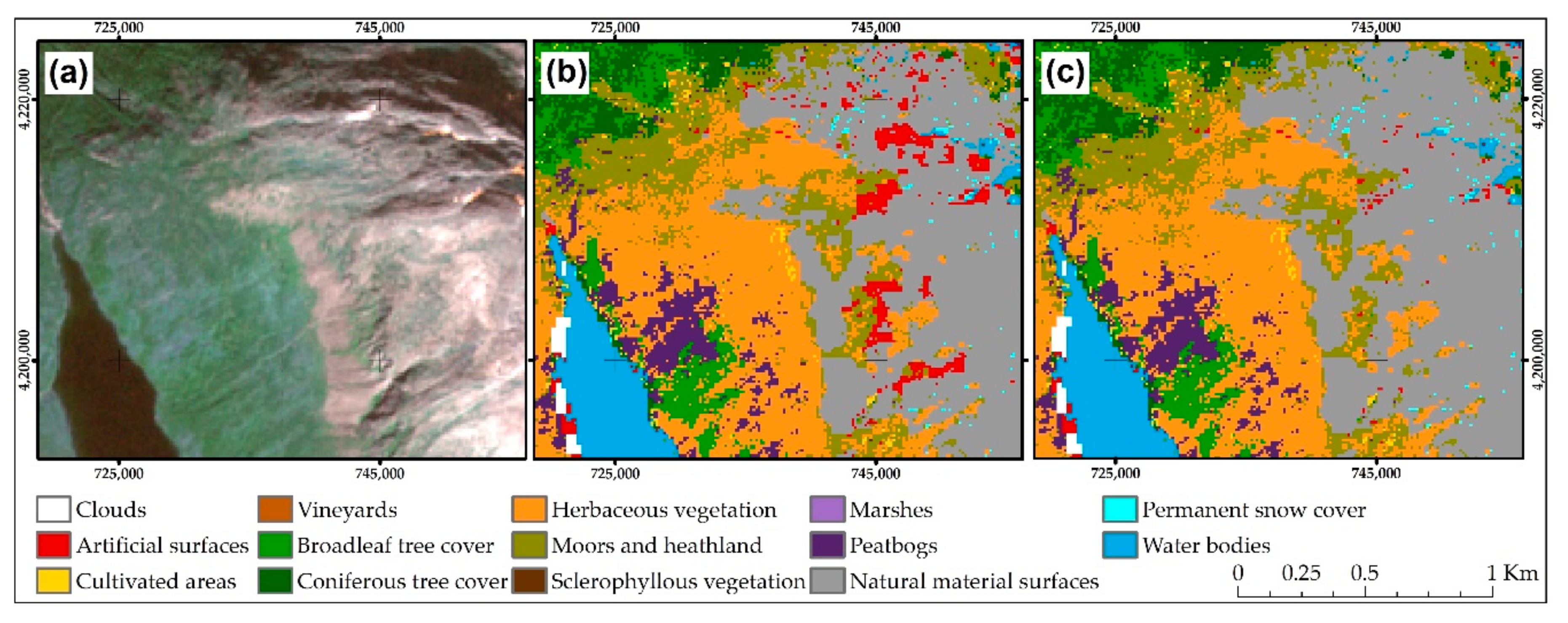
The post-processing procedure is an integral part of the workflow, and was designed to correct common classification errors. It was applied primarily to the artificial surfaces class, and thus most changes were found for this class, simultaneously increasing its mapping accuracy (i.e., an increasing of F1 score by 7%). Although our automated rules corrected a number of classification errors, the difference in OA with and without post-processing is not significant (an increase of 0.3%). However, visually the final classification map has been improved, especially in urban and mountainous areas.
Figure 8 presents a comparison of results before and after post-processing for a mountainous area in Norway, and illustrates the reduction in the number of misclassified pixels for the artificial surfaces class. This figure also highlights the problem of correct land cover class recognition in mountains. The spectral similarity between rock and artificial surfaces, along with numerous shadows, rapid changes in altitude, and the aspect of slopes, make mountain areas one of the most difficult regions to map accurately [
59].
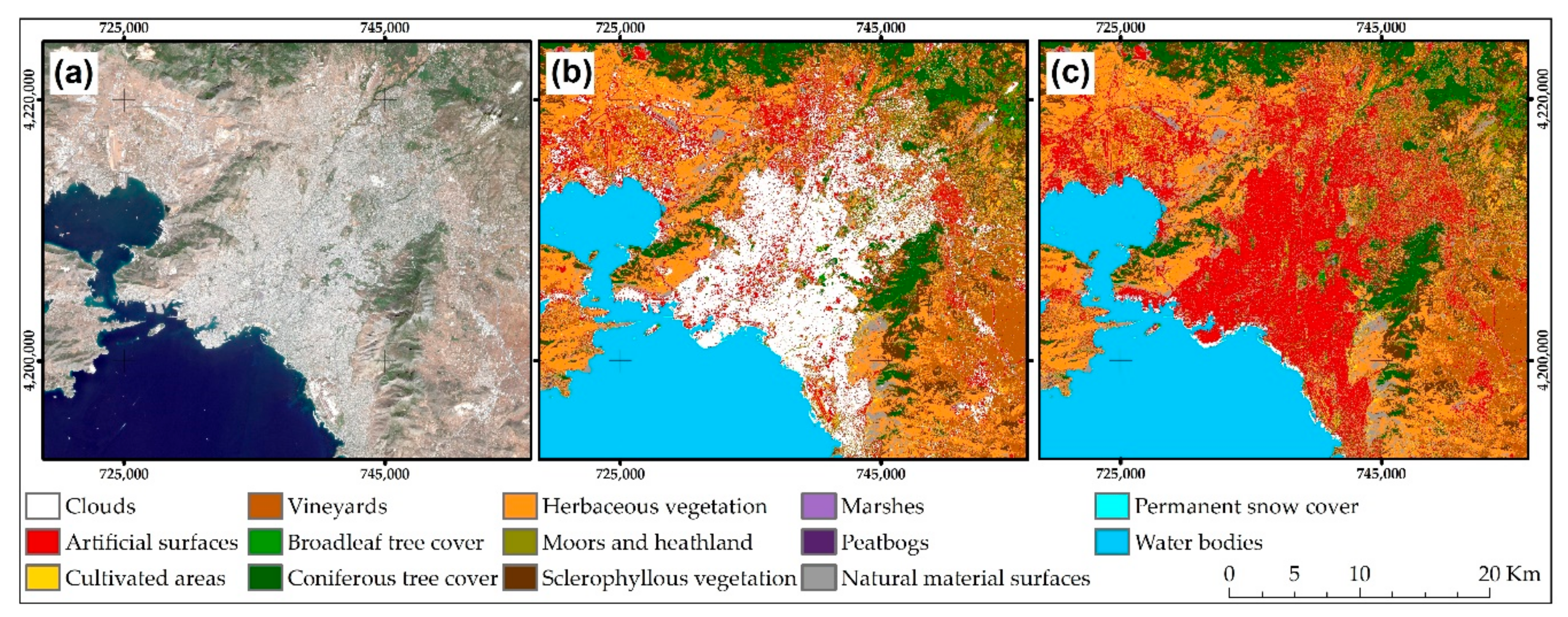
Figure 9 illustrates the positive changes resulting from the application of post-processing to a data subset representing urban areas of the city of Athens.
The development of our post-processing rules required the determination of exact thresholds for the posteriori class probability and elevation. This was based on the manual verification of values in numerous locations across Europe, which aimed to find thresholds that would best-fit the entire study area. Therefore, it would be necessary to determine new thresholds before applying the method to other areas or continents. Once specified, however, these thresholds can be applied automatically to all analysed tiles, improving the classification.
Finally, we found that posteriori class probability data generated by the random forest classification was very useful in improving land cover classification during post-processing [
11]. The application of information originating from the posteriori class probability allowed us to focus only on certain, potentially erroneous areas (pixels), and prevented the modification of correctly classified pixels.
4.5. Regional Class Differences
The spectral signature of some land cover classes may vary in different regions of an analysed area [
1,
59]. This particularly concerns vegetation classes that may be composed of different plant species (e.g., different broadleaf tree species), or be maintained under different land management systems (e.g., agricultural areas) [
58,
72]. To address this issue, and account for geographic variation in land cover class signatures, our approach performs locally adaptive classification [
3,
58] through the individual analysis of Sentinel-2 images, on a tile-by-tile basis. Here, we assume that a single tile (110 × 110 km) is sufficient to account for changing climatic conditions and phenological differences. This approach forces the classifier to learn locally, without aggregating class characteristics from large geographic regions. It also helps to reduce discrepancies in atmospheric correction between neighbouring areas (tiles), and to prevent the transfer of training-related classification errors from one area (Sentinel-2 tile) to other regions. Phenological differences are also taken into consideration by the classification of individual time series images, which approach enable and enforce, in fact, application of multi-seasonal training set. Such a strategy can account for the current state of vegetation, and avoids the need to generalise or average phenological characteristics.
5. Conclusions
This study presents details of a large-scale land cover classification workflow, and illustrates its application to a study area covering the majority of the European continent. It demonstrates that the thematic accuracy of our method is at least comparable to (or higher than) current techniques that use a training dataset derived from the visual interpretation of remote sensing data. It shows that even relatively outdated databases, with coarser resolution than the image being classified, may be an effective source of training samples, and enable mapping with high thematic accuracy. The method is enhanced by the efficient random forest machine learning classifier, which is highly resistant to noise in training data. Moreover, the selection of an independent training set for each classified image eliminates the need for training characteristics to be transferrable between areas that may have different spectral signatures for the same class.
Our method aims to fill a research gap addressing the problem of automatic, large-scale land cover classification, with an emphasis on the fully automatic generation of a training dataset. Furthermore, we demonstrated the application of an alternative method for the analysis of multi-temporal data.
The satisfactory performance of our method was confirmed using an appreciable validation dataset that made it possible to carry out a reliable assessment on both continental and country levels. Like in other studies, accuracy varies, with some classes having an F1 score above 0.9, while others perform below expectations. The latter requires further investigation, and improvements are needed to create an even more robust classification workflow.
An important aspect of our methodology is that it combines all data processing steps, enabling detailed mapping with no need for user intervention. The operability of the method is enhanced by the application of the DIAS computing environment, which facilitates both access to Sentinel-2 imagery and data processing.
The methodology presented in our study could be developed into a fully automated classification service, able to provide maps composed of basic land cover classes at a relatively high (e.g., annual) frequency. Such an automated and computationally efficient service could supplement existing land monitoring services and provide valuable input when analyzing environmental changes.

 ,
, 


