Article

Individual Tree Attribute Estimation and Uniformity Assessment in Fast-Growing Eucalyptus spp. Forest Plantations Using Lidar and Linear Mixed-Effects Models

by
Rodrigo Vieira Leite
1,*,
Carlos Alberto Silva
2,3,
Midhun Mohan
4,
Adrián Cardil
5,
Danilo Roberti Alves de Almeida
6,
Samuel de Pádua Chaves e Carvalho
7,
Wan Shafrina Wan Mohd Jaafar
8,
Juan Guerra-Hernández
9,10,
Aaron Weiskittel
11,
Andrew T. Hudak
12,
Eben N. Broadbent
13,
Gabriel Prata
13,
Ruben Valbuena
14,
Hélio Garcia Leite
1,
Mariana Futia Taquetti
1,
Alvaro Augusto Vieira Soares
15,
Henrique Ferraço Scolforo
16,
Cibele Hummel do Amaral
1,
Ana Paula Dalla Corte
17 and
Carine Klauberg
18
1
Department of Forest Engineering, Federal University of Viçosa, Viçosa, MG 36570-900, Brazil
2
Department of Geographical Sciences, University of Maryland, College Park, MD 20740, USA
3
School of Forest Resources and Conservation, University of Florida, Gainesville, FL 32611, USA
4
Department of Geography, University of California—Berkeley, Berkeley, CA 94709, USA
5
Tecnosylva, Parque Tecnológico de León, 24009 León, Spain
6
Department of Forest Sciences, University of São Paulo, “Luiz de Queiroz” College of Agriculture (USP/ESALQ), Av. Pádua Dias, 11, Piracicaba, SP 13418-900, Brazil
7
College of Forestry, Federal University of Mato Grosso, Av. Fernando Correa da Costa, 2367, Boa Esperança, Cuiabá, MT 78060-900, Brazil
8
Earth Observation Centre, Institute of Climate Change, National University of Malaysia (UKM), Bangi 43600, Malaysia
9
Centro de iniciativas empresariais, Fundación CEL. O Palomar s/n, 27004 Lugo, Spain
10
Forest Research Centre, School of Agriculture, University of Lisbon, Instituto Superior de Agronomia, 1649-004 Lisboa, Portugal
11
Center for Research on Sustainable Forests, University of Maine, 5755 Nutting Hall, Orono, ME 04469, USA
12
US Forest Service (USDA), Rocky Mountain Research Station, RMRS, 1221 South Main Street, Fort Collins, CO 80526, USA
13
Spatial Ecology and Conservation Lab, School of Forest Resources and Conservation, University of Florida, Gainesville, FL 32611, USA
14
School of Natural Sciences, Bangor University, Bangor LL57 2W, UK
15
Institute of Agricultural Sciences, Federal University of Uberlândia, Monte Carmelo, MG 38500-000, Brazil
16
Department of Forestry and Environmental Resources, North Carolina State University, Raleigh, NC 27695, USA
17
Department of Forest Engineering, Federal University of Paraná, Curitiba, PR 80210-170, Brazil
18
Department of Forest Engineering, Federal University of São João Del Rei, Sete Lagoas, MG 35701-970, Brazil
*
Author to whom correspondence should be addressed.
Remote Sens. 2020, 12(21), 3599; https://0-doi-org.brum.beds.ac.uk/10.3390/rs12213599
Submission received: 13 October 2020 / Revised: 26 October 2020 / Accepted: 29 October 2020 / Published: 2 November 2020
(This article belongs to the Special Issue Applications of Individual Tree Detection (ITD))

Abstract

:
Fast-growing Eucalyptus spp. forest plantations and their resultant wood products are economically important and may provide a low-cost means to sequester carbon for greenhouse gas reduction. The development of advanced and optimized frameworks for estimating forest plantation attributes from lidar remote sensing data combined with statistical modeling approaches is a step towards forest inventory operationalization and might improve industry efficiency in monitoring and managing forest resources. In this study, we first developed and tested a framework for modeling individual tree attributes in fast-growing Eucalyptus forest plantation using airborne lidar data and linear mixed-effect models (LME) and assessed the gain in accuracy compared to a conventional linear fixed-effects model (LFE). Second, we evaluated the potential of using the tree-level estimates for determining tree attribute uniformity across different stand ages. In the field, tree measurements, such as tree geolocation, species, genotype, age, height (Ht), and diameter at breast height (dbh) were collected through conventional forest inventory practices, and tree-level aboveground carbon (AGC) was estimated using allometric equations. Individual trees were detected and delineated from lidar-derived canopy height models (CHM), and crown-level metrics (e.g., crown volume and crown projected area) were computed from the lidar 3-D point cloud. Field and lidar-derived crown metrics were combined for ht, dbh, and AGC modeling using an LME. We fitted a varying intercept and slope model, setting species, genotype, and stand (alone and nested) as random effects. For comparison, we also modeled the same attributes using a conventional LFE model. The tree attribute estimates derived from the best LME model were used for assessing forest uniformity at the tree level using the Lorenz curves and Gini coefficient (GC). We successfully detected 96.6% of the trees from the lidar-derived CHM. The best LME model for estimating the tree attributes was composed of the stand as a random effect variable, and canopy height, crown volume, and crown projected area as fixed effects. The %RMSE values for tree-level height, dbh, and AGC were 8.9%, 12.1%, and 23.7% for the LFE model and improved to 7.3%, 7.1%, and 13.6%, respectively, for the LME model. Tree attributes uniformity was assessed with the Lorenz curves and tree-level estimations, especially for the older stands. All stands showed a high level of tree uniformity with GC values approximately 0.2. This study demonstrates that accurate detection of individual trees and their associated crown metrics can be used to estimate Ht, dbh, and AGC stocks as well as forest uniformity in fast-growing Eucalyptus plantations forests using lidar data as inputs to LME models. This further underscores the high potential of our proposed approach to monitor standing stock and growth in Eucalyptus—and similar forest plantations for carbon dynamics and forest product planning.

Graphical Abstract

1. Introduction

Forest plantations cover approximately 7% of the global forested area, including around 80 million ha in tropical and subtropical countries, and Eucalyptus spp. is one of the most widely cultivated species due to their fast growth rate [1,2,3]. In the context of sustainability, these plantations help to offset natural forest exploitation, restore some ecological services offered by natural forests, and mitigate climate change by storing carbon [4,5,6]. As economic endeavors, careful monitoring of forest plantation growth and productivity is critical for efficient and optimal management, with the objective of generating maximal yields while minimizing production costs and environmental disturbances. From a manager perspective who has to deal with large areas, having detailed information is necessary for this purpose and spatial modeling using remotely sensed data in fine resolutions could be useful in this regard.
Several remote sensing technologies have been used for forest monitoring in the past couple of decades. They provide comparable forest attributes estimations to traditional field survey-based methods while being less laborious and highly time-efficient, especially for areas that are difficult to access [7,8,9]. Light Detection and Ranging (lidar) has gained popularity among the remote sensing methodologies due to its ability to provide accurate and high-resolution 3D measurements of the forest. Airborne lidar data are well suited to calculate and/or predict forest structure attributes such as tree height [10,11,12], diameter at breast height (dbh) and basal area [13,14], stem volume [15,16] and aboveground biomass [17,18,19]. Many of the aforementioned applications have already been studied in the case of Eucalyptus plantations [20,21,22], although more attention needs to be given to the aboveground carbon (AGC) dynamics across different ages [8,23]. AGC information is important to understand the contribution of these forests in CO2 sequestration, and its incorporation into management plans will help to mitigate climate change [24,25,26].
Modeling and mapping forest attributes using lidar are primarily based on either the area or individual tree-based approaches. In the former, forest attributes are estimated to an area level (e.g., mean canopy height and volume in a plot), whereas the individual tree approach estimates the attributes for each tree (e.g., tree height, dbh, and volume) [9,22,27]. The area-based approach has been more commonly used in forestry applications as it is comparatively more straightforward to integrate with conventional inventory measurements and works with less expensive small-footprint lidar data [28]. However, detailed forest information, such as tree counts, stem height, dbh, and tree biomass, is essential for effective management and quantitative analysis of forests, so the tree-level approach is highly appealing from an inventory standpoint [29,30,31,32]. Therefore, effectively modeling of the attributes at the tree level needs to be explored together with its auxiliary information (e.g., stem distribution and location) for understanding the real impact of this approach on improving management decisions [33].
Tree-level attribute modeling using lidar data are carried out by using allometric relationships between lidar-derived crown metrics (e.g., tree height, crown volume, crown area) and a field observed variable (e.g., tree volume). In Eucalyptus plantations, other critical factors may be considered, such as: (a) hierarchical structure (e.g., plots within forest stands, forest stands within regions, repeated measurements of trees) and (b) crossed grouping structures (e.g., species and genotype variation) [34,35,36]. These may occur due to the measurement of sample plots from multiple stands with different characteristics to generate a representative dataset for model fitting. In these cases, linear mixed-effects models (LME) are found to be more flexible, precise, and accurate compared to ordinary linear fixed-effects models (LFM) [37,38]. LME models account for “random effects” and therefore enable multiple models for different sites and genotypes. The LME assumption is that the individual-specific effects and the independent variables are uncorrelated [39,40]. LME models fitted with data from lidar-supported inventories have been applied to Eucalyptus stands before, with the primary focus being site index and volume estimation at the plot level [34,41,42,43,44,45]. Nonetheless, combined individual tree level data and mixed-effect models have not been rigorously tested in fast-growing Eucalyptus plantations.
The tree-level estimations allow us to directly retrieve spatial distribution and uniformity of trees across the stand. In Eucalyptus plantations, this information is essential as stand heterogeneity may decrease productivity due to the impact of competition in tree yield [46,47,48]. Accurately identifying heterogeneous areas may also be used as a proxy for defining harvest and thinning goals [49]. One of the methods that have been used to assess tree uniformity is the Lorenz curves and Gini coefficient [50,51,52,53]. These methods have been mostly used with lidar to estimate plot-level forest structure in pine [53,54] and mixed-species [55] stands. However, it is still necessary to explore their application on lidar derived tree-level estimations in Eucalyptus-type stands, which are very different from pines.
In order to provide solutions for increasing forest plantation industry efficiency in monitoring and managing forest resources, the overall goal of this study was to develop and test a novel framework for modeling individual tree attributes, such as height, dbh, and AGC in fast-growing Eucalyptus stands using lidar-derived crown metrics and LME statistical modeling approach. We hypothesized a possible gain in accuracy over conventional LFM models given the known hierarchical structure of the field-measured data in these forest plantations. Herein, we also assessed forest uniformity across different stand ages using the Lorenz curves and Gini coefficient based on the tree-level estimated attributes from the best-fitted LME model. In addition, we discussed the implications of our framework for management decisions and precision forestry.

2. Materials and Methods

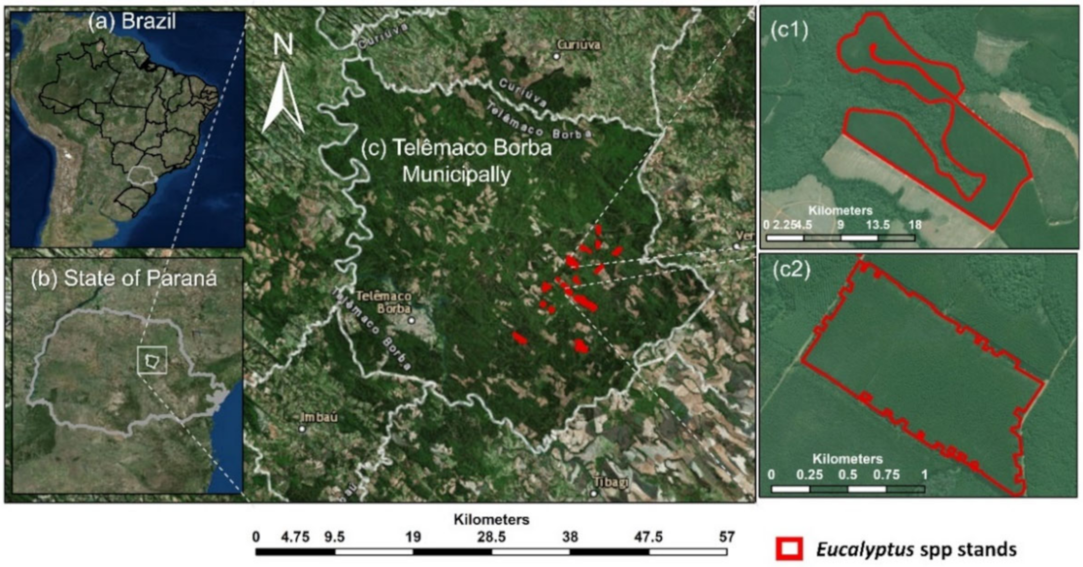
2.1. Study Area Description

The study area was located in southern Brazil within the Telêmaco Borba municipality in the state of Paraná (Figure 1), and it is owned by a pulp and paper company. There were 23 Eucalyptus stands where eight species and five genotypes were planted. Each stand was planted with a single genotype (i.e., stands were single-species and single-genotype). The stands managed to meet the company standards of high productivity and were free from significant damage from fire, disease, or insects. Trees were planted using a 3 × 3 m grid configuration, resulting in an average tree density of 1111 trees/ha. The site is characterized by an average altitude of 741 m with a relatively flat slope, annual average precipitation of approximately 1378 mm, and an annual average temperature of 18.4 °C [56].

2.2. Field Data Collection

A total of 25 rectangular (20 × 30 m; 600 m2) plots were randomly established such that the sample plots represented the study area in an unbiased manner and captured forest variability among stands (summary of the plots is presented in Table S1). Individual trees were measured for diameter at 1.3 m above the ground (dbh), and a random subsample of 15% of the trees inside each plot was measured for total height (Ht). Tree heights that were not directly measured were estimated using hypsometric equations employing dbh as the independent variable [57], resulting Ht estimates with mean ± standard deviation (sd) bias of −0.03 ± 0.04 m (−0.23 ± 0.3%). Herein, plot locations were georeferenced using a decimeter accuracy differentially corrected geodetic GNSS (Trimble Pro-XR). Information regarding species, age, and genotype were also noted. AGC (kg/tree) was obtained through an allometric model, employing the logarithm of dbh and Ht as independent variables, based on an approach developed in [9] (see Supplementary Material). In summary, the stand ages ranged from 1.7 to 4.3 years, and the mean ± sd of the stand attributes Ht, dbh, AGC, and age were 16.09 (±3.68 m), 13.46 (±2.65 cm), 33.04 (±14.61 kg/tree), and 3.04 (±0.74 years), respectively.

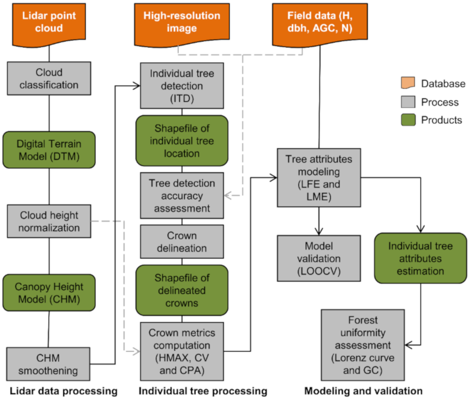
2.3. Lidar Data Acquisition and Pre-Processing

Lidar data and high-resolution imagery were acquired at the same period of field data collection using a Harrier 68i system mounted on a CESSNA 206 aircraft in 2012. The lidar flight parameters are presented in Table 1. Digital Terrain Model (DTM), canopy height model (CHM), and lidar-derived crown metrics were the main products derived from lidar data processing and were created using the US Forest Service FUSION/LDV 4.0 software [58]. First, ground points were identified in the raw 3D point cloud data using Kraus and Pfeifer’s algorithm [59], from which a 1 × 1 m resolution DTM was generated using the GridSurfaceCreate function. The height of each raw point was then computed using the Clipdata tool, and a 0.5 × 0.5 m CHM raster was generated using the CanopyModel. The points were then clipped in 3D to the sample plots using the ClipData tool. Lidar crown-level metrics were computed on this final height-normalized all-returns point cloud (item 2.4).

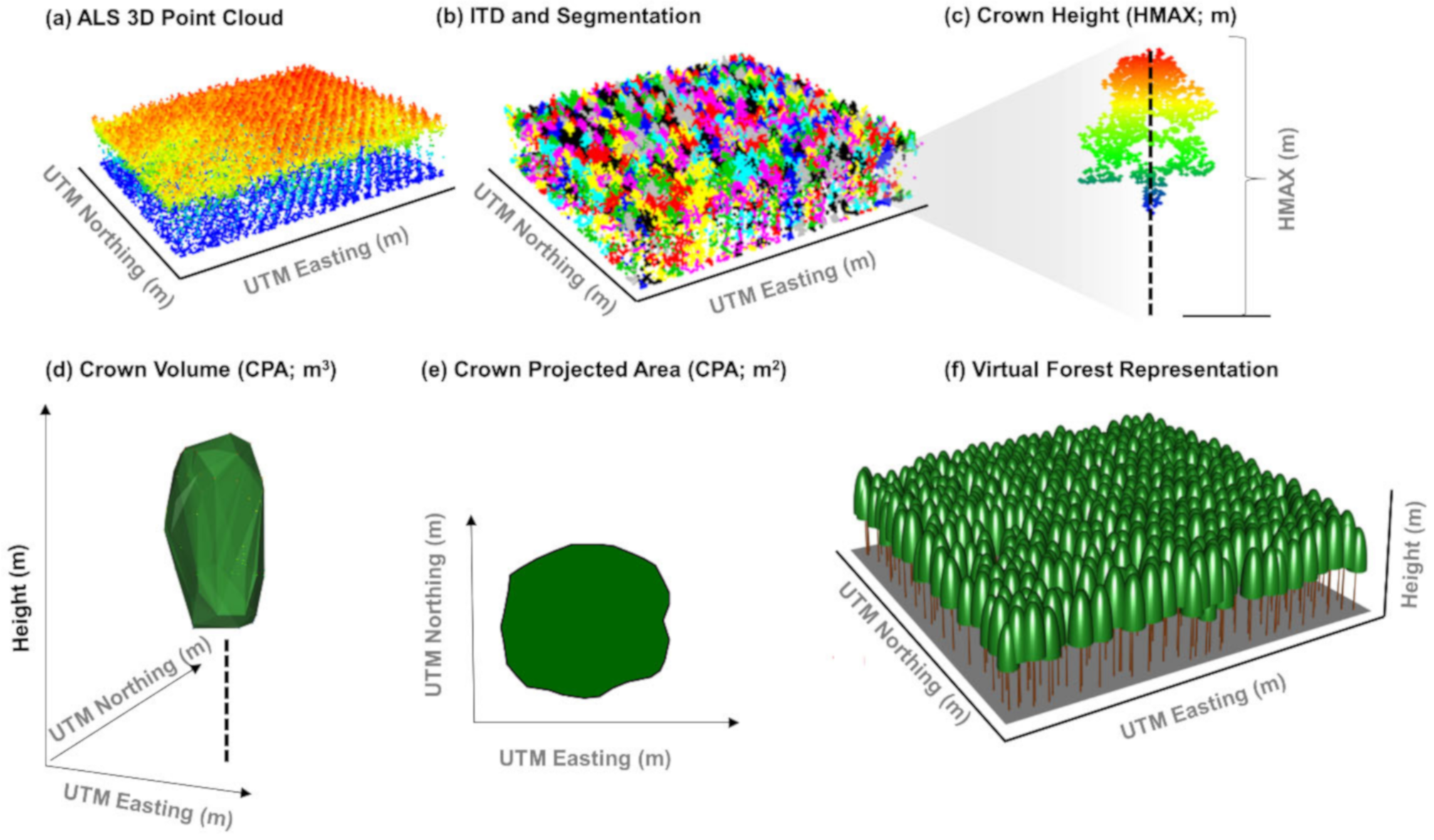
2.4. Individual Tree Detection and Crown Metrics Computation

The first step in the tree-based approach is to detect and delineate individual trees. The individual tree detection was performed by applying algorithms to the CHM rasters using the rLiDAR package [60] in R [61]. The entire process consisted of 5 core steps: (1) smoothing the CHM with a 3 × 3 mean filter to remove spurious local maxima caused by tree branches, (2) tree top detection from the smoothed CHM using the local maxima algorithm of the FindTreeCHM function (a 5 × 5 window was used in this case), (3) delineation of tree crowns using the Voronoi Tessellation algorithm based on the ForestCAS function, iv) extraction of all returns of the normalized 3D point cloud within the tree crowns, and v) computation of crown-level metrics—maximum height (HMAX, m), crown projected area (CPA, m2), and crown volume (CV, m3) for individual trees using the CrownMetrics function (Figure 2). We assumed that these three metrics would be relevant for the tree attributes modeling based on observations made in previous studies [62,63]. In the accuracy assessment, we compared the number of lidar-detected trees per plot with the numbers of trees observed in the field and verified the tree location and crown boundary by overlaying it on the high-resolution RGB image.

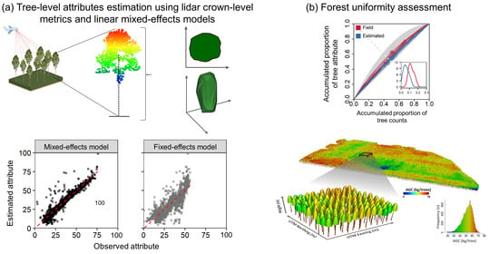
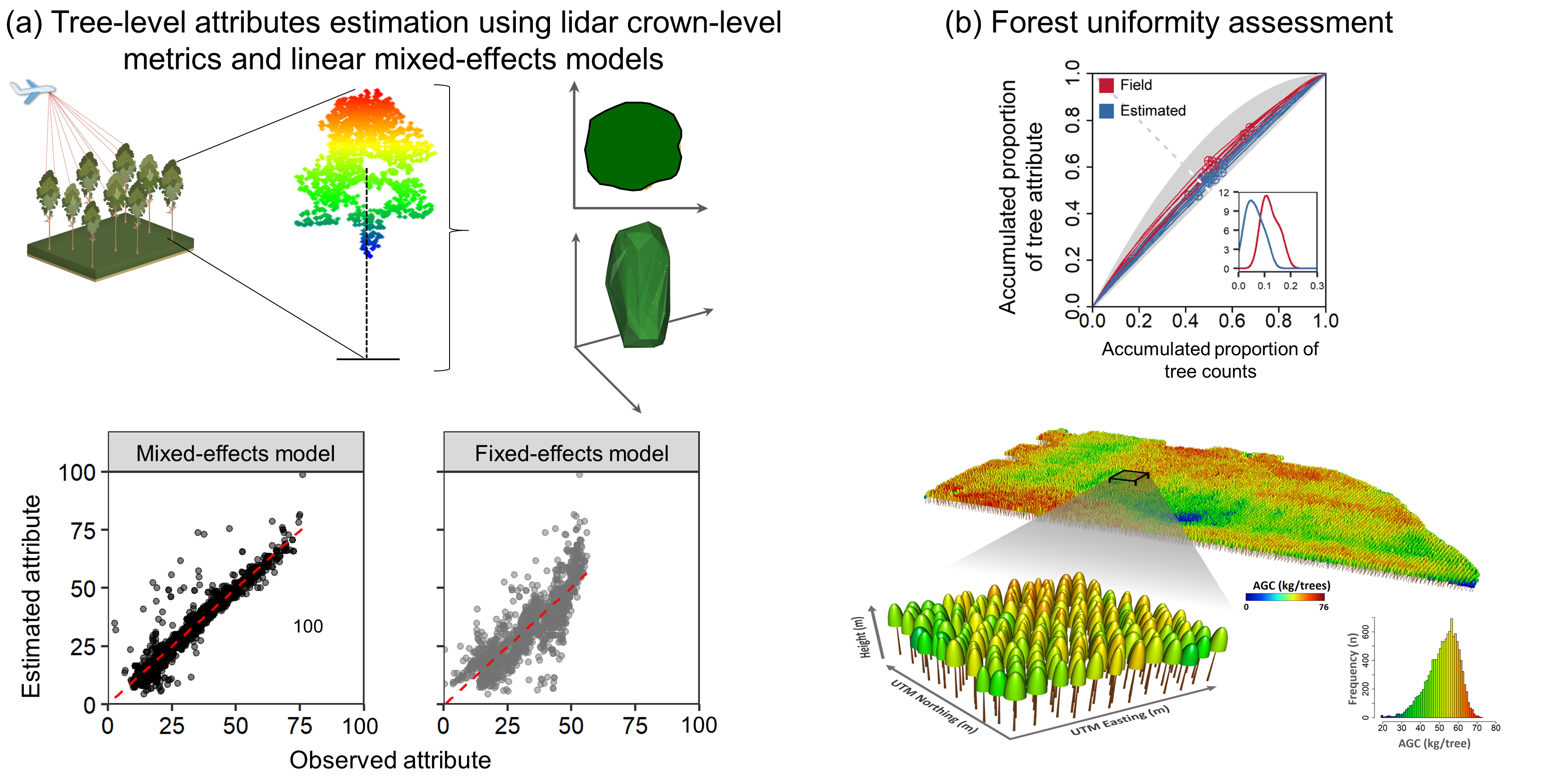
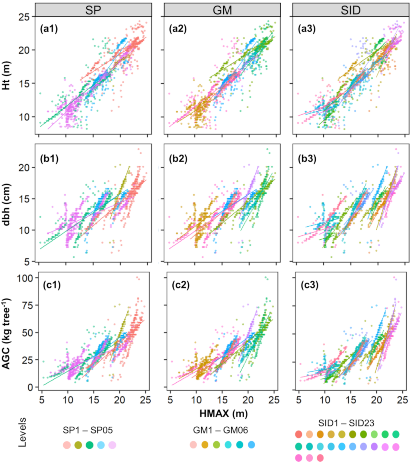
2.5. Individual Tree Attribute Modeling

To model the tree attributes (i.e., Ht, dbh, and AGC), we spatially linked the field and lidar-detected individual trees within each plot. A total of 1520 reference trees were used, and a preliminary exploratory analysis was conducted using scatterplots and correlation coefficient to identify trends in the data. In all models, the independent fixed-effects variables were the lidar-derived HMAX, CPA, and CV. To accommodate the potential random nature of the variables that were visible during the graphical analysis stage, four LME models [37,38] were developed to estimate the three dependent attributes with varying intercept and slope. The first three models were built using the tree species (SP), genotype (GM), and stand (SID) separately as random-effects variables, and the fourth was built using them in a nested structure. The models were fitted using the lmer function in the “lme4” R package [64]. The general expression of the LME is presented in Equations (1) and (2).
Y   =   X β + Z u + ε
where: Y is the vector of response variables; β is the vector of fixed effects; u is the vector of random effects with E(u) = 0 and u~N(0, σ u 2 D); ε is the vector of residuals with E(ε) = 0 and ε ~ N(0, σ ε 2 I); X and Z are design matrices relating the observations y to β and u, respectively.
Y i j   =   β 0 +   u 0 i j + β 1 +   u 1 i j   HMAX i j + β 2 +   u 2 i j   CPA i j + β 3 +   u 3 i j CV i j + ε i j
where: Yij is the response variable for the i-th tree; β 0 and u 0 i j are the fixed and random intercepts, respectively; β 1 , β 2 ,   β 3 are the fixed coefficients associated to HMAX, CPA, and CV, respectively; u 1 i j , u 2 i j ,   u 3 i j are the random coefficients for the i-th tree and random-effect variable j; ε i j is the random error with E(ε) = 0 and ε i j ~ N(0, σ ε 2 I).
The results were compared with a conventional linear fixed-effect model (LFE) with the same fixed-effects (i.e., independent variables HMAX, CPA, and CV) used in the LME models (Equation (3)). The LFE provided a model based on only fixed effects to test whether including random effects in the LME model significantly improved the results. The R lm function [65,66] was implemented for this purpose. The models were tested for normality and heteroscedasticity of the residuals with the Shapiro–Wilk [67] and Breusch–Pagan tests [68], respectively, for a stand-based estimate.
Y i   =   β 0 + β 1   x   H M A X i +   β 2   C P A i +   β 3   C V i +   ε i ,
where: Yi is the response variable of the i-th tree; β 0 , β 1 , β 2 , β 3 are the intercept and slope parameters associated with the lidar-derived variables HMAX, CPA, and CV, respectively; ε i is the random error with E(ε) = 0 and ε i ~ N(0, σ ε 2 I).
The accuracy of each model was assessed according to the coefficient of determination (R2), absolute and relative root mean square error (RMSE and %RMSE, respectively), and absolute and relative bias (%bias) (Equations (4)–(8), respectively). The Akaike information criterion (AIC) was also calculated for comparing and ranking the proposed models [69,70]. To validate the model performance, we computed the aforementioned statistics again using a leave-one-out cross-validation (LOOCV). The acceptable precision was considered to be a %RMSE below 15% and bias near to zero to satisfy conventional forestry inventory standards [23].
R 2   = 1   i   =   1 n Y ^   Y i i 2 i   =   1 n Y i   Y ¯ 2 ,
R M S E   = i   =   1 n Y i ^   Y i 2 n ,
% R M S E   =   R M S E Y ¯   ×   100 ,
b i a s   =   i   =   1 n Y ^ i   Y i n ,
% b i a s   =   b i a s Y ¯   × 100 ,
where: Y i ^ = estimated tree attribute for the i-th tree; Y i = observed tree attribute for the i-th tree; Y = observed mean tree attribute; n = number of observations.

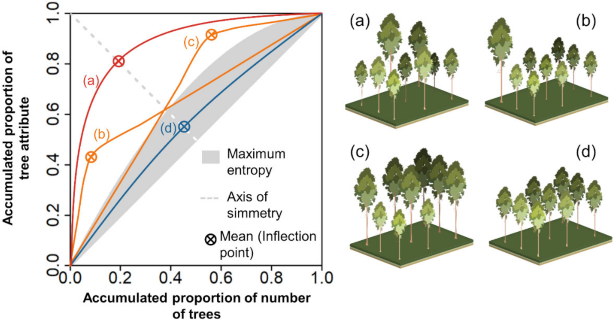
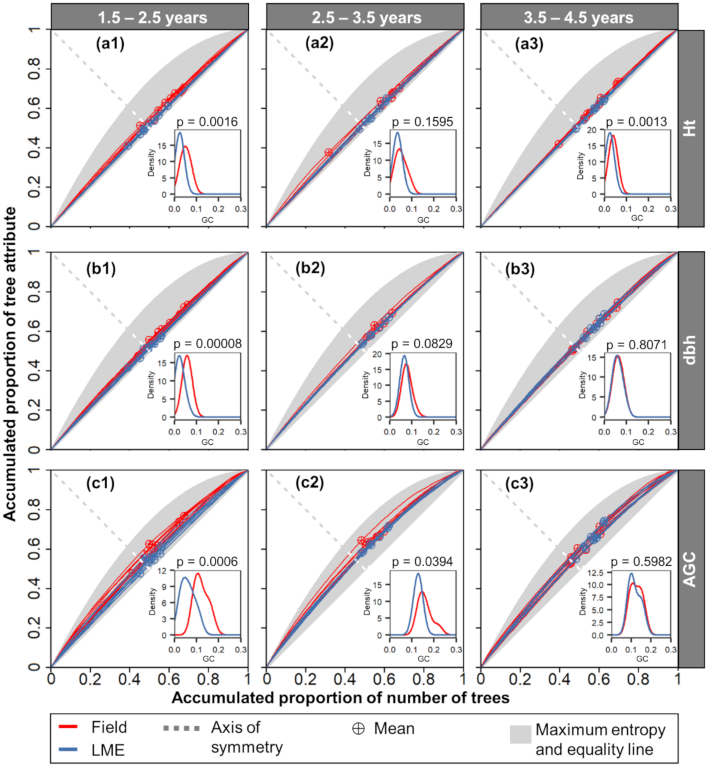
2.6. Assessing Forest Attributes Uniformity

Field and best-fitted LME model derived tree attributes were used to assess forest uniformity at the plot level. Herein, we used the Lorenz curve and Gini coefficient (GC) for their interpretability in describing forest structural differences in terms of uniformity of tree sizes [50,52,53,71]. We calculated the Lorenz curve and GC for describing the uniformity of the three estimated attributes (i.e., Ht, dbh, and AGC). The indices were calculated using the estimated values, and field measurements and the GC values were compared using the two-tailed Student’s t-test. The plots were also split into the age classes of 1.5–2.5, 2.5–3.5, and 3.5–4.5 years for observing if the uniformity patterns changed for different ages. In the calculation, the trees were ranked in decreasing order with the intention to depict the dominance of larger trees in the y-axis [46,52], and the Lorenz curves were built by plotting the cumulative percentage of trees against the cumulative percentage of each tree attribute. The GC was then calculated as the ratio of the area contained under the empirical Lorenz curve by the area above the diagonal line of perfect equality (when all trees are identical in size). The GC thus theoretically ranges from 0 (all trees of equal size) to 1 (highest theoretical dispersion where only one observation holds the sum of the attribute against many tree sizes which are negligible, e.g., by not reaching the breast height). In forest science, the Lorenz curves are compared against the Lorenz curve of maximum entropy (depicted by a grey area in Figure 3), which represents the most uneven-sized situation with trees ranging from all types of sizes [52]. Adnan et al. [72] showed that maximum entropy could be deducted for fixed threshold values of GC. The authors demonstrated that these thresholds are different depending on whether the tree attributes used are one-dimensional (e.g., tree height or dbh) or two-dimensional (e.g., basal area or crown area) measures and determined the thresholds GC = 0.33 (one-dimensional) and GC = 0.50 (two-dimensional) which correspond respectively to each of the aforementioned groups. Accordingly, in this research, we employed a threshold of GC = 0.33 to depict the maximum entropy (i.e., plots with GC values below the threshold were considered as single-cohort even-sized forests) [72]. Moreover, the inflection point of the Lorenz curve depicts the mean value of the tree attribute [51,71,73]. The possible theoretical scenarios for describing the stands are uneven-sized stands with balance among tree cohorts (i.e., symmetric; Figure 3a), uneven-sized stands with a dominance of small trees (i.e., negatively asymmetric; Figure 3b), or dominance of large trees (i.e., positively asymmetric; Figure 3c) and even-sized stands with all trees of roughly the same size (curves that fall below the curve of maximum entropy, within the grey-shaded area—Figure 3d). Figure 4 offers a synopsis of the complete methodological workflow.

3. Results

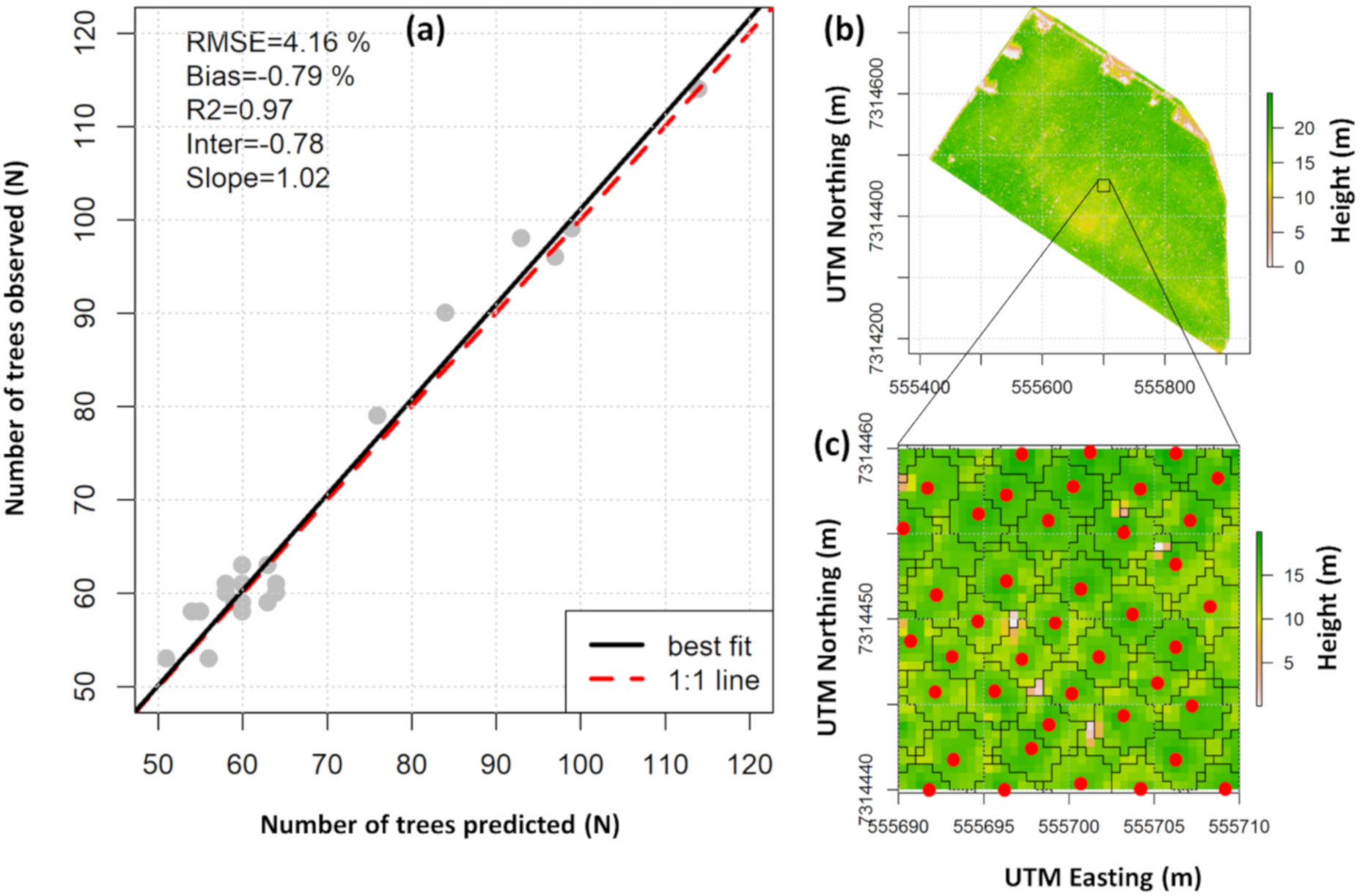
3.1. Individual Tree Detection and Crown Metrics

From the 1520 reference trees, 1468 (96.6%) were correctly detected (missed trees = 20; falsely detected trees = 32). A 1:1 comparison of the number of field-observed and lidar-detected trees by plot shows %RMSE and %bias less than 5% and 0.8%, respectively (Figure 5a).
When assessing the lidar-derived crown-level metrics (Table S2), we found HMAX to be highly correlated (r > 0.78) with the response variables, whereas CV and CPA showed very low correlations (r < 0.3). This is further highlighted when analyzing the scatterplots between HMAX and field attributes across the random-effect variables (Figure 6).

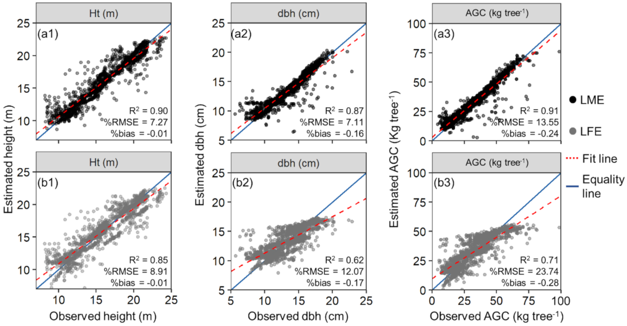
3.2. Predictive Models

Overall, the LME performed better than the LFE models (Table 2). The most accurate LME was built with the SID as a random-effect variable. The fitted equations using SID as a random-effect variable for Ht, dbh, and AGC explained 90%, 87%, and 91% of the attribute’s variation, respectively, while the LFE models only did 84%, 62%, and 71% for the same tree attributes. The latter models also satisfied residual normality and homoscedasticity assumptions for the stand estimations (W > 0.83 and p-value > 0.09 in the Shapiro–Wilk test, and BP > 1.6 and p-value > 0.13 in the Breusch–Pagan test). Even though the LME with nested SID, SP, and GM had very similar results to using only SID, it lacked simplicity, as shown by the AIC values—9131.3 for the former and 9119.3 for the latter. Therefore, the LME model with SID as a random-effect was selected for the subsequent analyses. In all the best-fitted LME, the random-effects were used in the intercept and HMAX-associated parameters only, as doing so for the other variables did not improve performance (Table S3). The HMAX was the most important variable in all models, as commonly seen in allometric models using lidar metrics [10], while CV did not contribute significantly to the models (p < 0.05). The CPA was not significant only for the Ht estimation with the LFE model.
The difference among LFE and the LME model with SID as a random-effect variable was also observed in the LOOCV assessment (Figure 7). The %RMSE decreased by approximately 1.5, 5, and 10 percent points for Ht, dbh, and AGC, respectively, when using the LME with SID as a random-effect variable rather than LFE. The differences in %bias were not as significant where the decrease was 0, 0.01, and 0.04 percent points with all models having a value lower than 0.3.
The Lorenz curves calculated from the field measurements and the best LME model estimations were overall similar (Figure 8). The main differences occurred in younger ages (1.5–2.5 years), especially for the AGC estimation. As expected, all the curves fell within the maximum entropy range. The mean attribute values (inflexion points checked with crossed symbol) of the younger stands were evenly distributed around the axis of symmetry (Figure 8a1,b1,c1). For stands of other ages, the values were mostly above this axis, representing a dominance of single cohorts of larger trees. The GC values all ranged around 0.1. Values slightly over 0.2 were found only in the coefficients calculated for the field measured AGC in the age classes 1.5–2.5 and 2.5–3.5 years. Significant differences between the GC using the field measurements and estimates with the LME with SID occurred mostly at the stands of 1.5–2.5 years, with the p-values being less than 0.002.

4. Discussion

Our study explored tree-level information from lidar for enhancing the forest management decision-making processes and underscores the importance of incorporating random effects while generating predictive models for individual tree attributes in forest plantations. Herein, linear mixed-effects models were found to outperform ordinary least square regression models, which only consider fixed effects. By demonstrating a forest uniformity estimation procedure, we hope to translate our research approach into future forest inventory practices and subsequently bolster ongoing data collection and production endeavors.
The application of the Silva et al. [60] algorithm for tree segmentation was able to detect more than 95% of the trees in our work. This constitutes an outstanding result when compared to other studies involving the tree individualization approach [74] and serves as an example of improvements to lidar-based forest inventory. This relatively new paradigm is therefore perfect for tree-level attribute estimation in Eucalyptus plantations where such in-depth detail is necessary for accommodating small-scale variations that are untraceable via plot-based estimation procedures [21,75,76,77,78,79]. Herein, the lidar-derived crown-metrics were found to provide a satisfactory estimation of Ht, dbh, and AGC, and the best results were obtained while employing a LME with SID as the random-effect variable. This variable is related to the site and would have likely enabled us to account for the existing grouping characteristics and growth variances of the tree attributes, improving the model performance. A similar trend was observed in several previous studies as well, where authors highlighted the better performance of LME models over LFE models [35,45,80,81]. One of the reasons might be related to the spatial correlation between the samples, which makes them not completely independent, and this introduces correlation into the model residuals [45,82,83]. This characteristic is not desired in LFE models [45,82,83]. On comparing our findings with similar studies in Eucalyptus stands, the major takeaway is that we were able to estimate forest attributes at the tree level and assess forest uniformity as opposed to only estimating forest attributes either at the tree or plot level. For instance, Packalen et al. [34] focused on using LME for estimating site index at the plot level, while Vauhkonen et al. [42] focused on evaluating and comparing area and tree-based lidar approaches for estimating stand volume with LME models in Eucalyptus plantations by applying genotype and stand as random-effect variables.
The lidar-derived crown-level metrics had different contributions in the models. The CPA and CV were not as important as the HMAX but were still found significant to most of the models. Previous studies provide some evidence that CPA and CV metrics might be important to biomass and other forest attribute estimations [62,63,84,85,86]. Crown-level field measurements are not commonly collected in Eucalyptus plantations but can be considered in further studies to infer their real impact for lidar-based allometric modeling in these forests. There is a cost (time and money) related to measuring CPA and CV variables in the field, and a more straightforward way as described by Maltamo et al. [86] could be obtaining only the canopy base height as a reference. The crown information could be an indicator of growth potential and tree health and give insights on stem quality and tree competition affecting tree growth. Therefore, crown-related metrics, although less important in our study, need to be further understood to be incorporated into tree attribute models in Eucalyptus plantations.
In Eucalyptus plantations, tree heterogeneity might not be desirable as unbalanced competition could affect tree yield especially when it is present at an early stage [32] and decrease stand productivity [46,47,48,87]. Identifying heterogeneous areas can aid forest managers in silvicultural decisions and growth modeling but is limited due to constraints associated with time, labor and financial needs; assessing it from remotely sensed detected trees becomes an alternative in such cases. Hentz et al. [88] reported that the errors incurred due to tree height calculation discrepancies do not significantly affect the uniformity index results given these errors are distributed evenly throughout the study area. Therefore, the concerns associated with individual tree detection are only the major ones to be noted while choosing between lidar and field-based studies. For plantation studies, such as ours, lidar-derived crown-level metrics were effective for calculating uniformity. However, the same might not be recommended in forests with more complex structures [73].
We used the Lorenz curves and GC to assess forest uniformity at tree level and found that the estimations fairly depicted the tree attributes variation, mainly in stands over 2.5 years. Trees in the given Eucalyptus stand were found to be quite similar, which was evident from the low values of GC (<0.33) and the close proximity of Lorenz curves to the perfect equality line in Figure 8. The differences found in younger stands may be related to errors associated with tree detection and crown delineation at this age, which is commonly the main source of errors in tree-level approaches [79,89]. Further research may clarify the relationships between the theoretical threshold GC < 0.33 [72] and productivity loss in Eucalyptus plantations. This will allow us to verify if the heterogeneity affects tree growth rates. Another important point to consider is the scale-factor associated with GC calculation. As described by Adnan et al. [90], GC tends to zero when assessed at a finer scale (i.e., using a considerably smaller plot), while at coarser scales, GC can increase asymptotically toward a maximum value that best describes the size heterogeneity of uneven-sized forests.
Despite the advantages of using lidar data for forest inventory, there is a cost-benefit trade-off associated with obtaining and processing data at more precise and fine-scale localized levels, which comes from lidar flight cost and hardware limitations (e.g., memory and processing); this should be circumventable in the long run given the continuing progress of science and technology. Even then, the scalability, reusability, and transferability of the proposed approach is expected to outweigh the capital cost limitations. For instance, the same LME models presented here could be easily recalibrated to become applicable to different SID levels coming from new field measurements [91,92,93] (example in the Supplementary Material). In addition, the lidar data bring the benefit of directly extrapolating the estimations for the entire area. Our results also inform that LME models are viable alternatives for scenarios where numerous levels need to be considered (e.g., different sites and genotypes), and stratifying the data may not be deemed feasible as it may lead to considerably fewer samples per level. Additionally, the same methods can be extended to other types of forest plantations as well for determining stand variability and/or for improving management decisions.
The novel framework presented in this study can be perceived as a step forward within the precision forestry realm if implemented [94]. Tree-level lidar studies are currently not undertaken at large-scale plantation areas. Yet, fine-scale attribute estimations and their uniformity can be delivered through the operationalization of the proposed approach (Figure 9). Such information allows localized silviculture treatments associated with irrigation, disease detection, growth imbalances, and pest control. This also enhances forest management efficiency as we would have better estimates of the attributes and variability within the stands. Presently, while performing forest inventories, several forest industrial companies use only a small number of randomly established plots (~1 every ~15–20 ha), and they can be placed in an unrepresentative region with respect to stand variability, and this can introduce bias into their forest attribute estimations. Thus, sampling plot allocation and concomitant costs can be optimized using lidar data [95,96,97,98]. For harvest planning, managers can use detailed information to estimate potential yield, harvest time, and volume stock for specific regions in the stand or define selective logging objectives [35]. Our strategy could also facilitate the application of individual-tree level growth and yield models, calculation of competition indices, identification of areas of low productivity (e.g., due to low soil fertility, pests, or disease), and identification of dominant trees for site index classification. It is worth mentioning that the resolution of the point cloud data used to achieve the results in this study was not as high as the currently available state-of-the-art lidar technologies. That might make it feasible to apply these methods to large areas at a lower cost. Given all the benefits in relation to large-scale spatialization, enhanced individual tree attributes estimation, and forest uniformity assessment, we expect our workflow to be implemented extensively in the coming years not only in Eucalyptus plantations but also in diverse species varieties globally.

5. Conclusions

In this study, we demonstrated that Ht, dbh, and AGC individual tree attributes could be accurately estimated in a fast-growing Eucalyptus forest plantation using lidar-derived crown-level metrics combined with LME models. Our framework also allowed assessing forest uniformity at the tree level using the LME model-derived estimates. The LME model using only the stand as a random-effect variable, was able to effectively account for the grouping variability characteristics of the data and resulted in the best model. This further highlights the importance of considering random effects into the modeling approach for estimating individual tree attributes in forest plantations, as the observations usually used are not completely independent due to, e.g., spatial correlation. Understanding these effects is important for supporting the development of robust models by incorporating sources of variation and reducing error in tree attribute estimations. By presenting a transferrable and scalable state-of-the-art approach that emphasizes the need to integrate spatial data with management decision-making processes, we hope to boost outreach capabilities of precision forestry-related endeavors worldwide.

Supplementary Materials

The following are available online at https://0-www-mdpi-com.brum.beds.ac.uk/2072-4292/12/21/3599/s1, Table S1: Descriptive statistics (mean ± standard deviation) of field measurements in the area of study. Ht = height; Dbh = diameter at 1.3 m above the ground; AGC = aboveground carbon, Table S2: Summary statistics of lidar derived crown-metrics maximum height (HMAX), crown projected area (CPA), and crown volume (CV), Table S3: Statistics for the linear mixed-effect model (LME) using the stand (SID) as random-effect variable considering intercept ( u 0 i j ) and slope ( u 1 i j , u 2 i j and u 3 i j ) combinations. RMSE = root mean square error, R2 = Coefficient of determination; AIC = Akaike information criterion, Figure S1: Scatterplot comparing recalibrated linear mixed-effect model and fixed-effect models (LME and LFE, respectively) for estimating aboveground carbon (AGC). R2 = coefficient of determination; %RMSE = relative root mean square error.

Author Contributions

All the authors have significantly contributed to the development of this study being involved in designing, drafting, and giving critical reviews. Conceptualization, C.A.S., C.K., A.T.H., M.M.; methodology, R.V.L., C.A.S., S.d.P.C.e.C., A.T.H., R.V., H.G.L., A.A.V.S., H.F.S.; validation, R.V.L, M.F.T., H.F.S., A.A.V.S., D.R.A.d.A., H.G.L.; formal analysis, M.M., A.C., D.R.A.d.A., W.S.W.M.J., J.G.-H., A.T.H., G.P., A.W., A.A.V.S.; data curation, R.V.L., C.A.S., M.F.T., R.V., H.G.L., A.A.V.S., H.F.S., C.K.; writing—original draft preparation, R.V.L., M.M., C.A.S., E.N.B., H.G.L, M.F.T., C.H.d.A., C.K., A.P.D.C.; writing—review and editing, M.M., E.N.B., A.C., W.S.W.M.J., J.G.-H., D.R.A.d.A., A.W., A.T.H., R.V., G.P., S.d.P.C.e.C., G.P., C.H.d.A., A.P.D.C.; visualization, R.V.L, C.A.S., D.R.A.d.A., A.P.D.C., R.V., H.F.S.; supervision, C.A.S., C.K., C.H.d.A., E.N.B., H.G.L.; project administration, C.A.S., C.K. All authors have read and agreed to the published version of the manuscript.

Funding

D. Almeida was supported by the São Paulo Research Foundation (#2018/21338-3 and #2019/14697-0). R. Leite was supported by the Coordination for the Improvement of Higher Education Personnel (CAPES - 88882.461705/2019-01). W.S.W.M Jaafar was supported by the National University of Malaysia (UKM) research grant GUP-2018-132.

Acknowledgments

The authors are very grateful for the lidar and field inventory data collections funded by Klabin S.A., a pulp and paper company. Thanks to Fernanda Leite for providing some of the tree figures used in the manuscript. We also acknowledge the financial support from the São Paulo Research Foundation, Coordination for the Improvement of Higher Education Personnel (CAPES), and National University of Malaysia (UKM).

Conflicts of Interest

The authors declare no conflict of interest.

References

  1. Payn, T.; Carnus, J.M.; Freer-Smith, P.; Kimberley, M.; Kollert, W.; Liu, S.; Orazio, C.; Rodriguez, L.; Silva, L.N.; Wingfield, M.J. Changes in planted forests and future global implications. For. Ecol. Manag. 2015, 352, 57–67. [Google Scholar] [CrossRef] [Green Version]
  2. Ibá, I.-I.B. De Árvores Report 2019; OSAC: São Paulo, Brazil, 2019. [Google Scholar]
  3. Carle, J.B.; Duval, A.; Ashfordc, S. The future of planted forests. Int. For. Rev. 2020, 22, 65–80. [Google Scholar] [CrossRef]
  4. Sedjo, R.A. The potential of high-yield plantation forestry for meeting timber needs. In Planted Forests: Contributions to the Quest for Sustainable Societies. Forestry Sciences; Springer: Dordrecht, The Netherlands, 1999; pp. 339–359. [Google Scholar] [CrossRef]
  5. Paquette, A.; Messier, C. The role of plantations in managing the world’s forests in the Anthropocene. Front. Ecol. Environ. 2010, 8, 27–34. [Google Scholar] [CrossRef] [Green Version]
  6. Roise, J.P.; Harnish, K.; Mohan, M.; Scolforo, H.; Chung, J.; Kanieski, B.; Catts, G.P.; McCarter, J.B.; Posse, J.; Shen, T. Valuation and production possibilities on a working forest using multi-objective programming, Woodstock, timber NPV, and carbon storage and sequestration. Scand. J. For. Res. 2016, 31, 674–680. [Google Scholar] [CrossRef]
  7. Næsset, E. Estimating timber volume of forest stands using airborne laser scanner data. Remote Sens. Environ. 1997, 61, 246–253. [Google Scholar] [CrossRef]
  8. Silva, C.A.; Klauberg, C.; Carvalho, S.; Hudak, A.T.; Rodriguez, L.C.E. Mapping aboveground carbon stocks using LiDAR data in Eucalyptus spp. plantations in the state of Sao Paulo, Brazil. Sci. For. 2014, 42, 591–604. [Google Scholar]
  9. Silva, C.A.; Hudak, A.T.; Vierling, L.A.; Loudermilk, E.L.; O’Brien, J.J.; Hiers, J.K.; Jack, S.B.; Gonzalez-Benecke, C.; Lee, H.; Falkowski, M.J.; et al. Imputation of Individual Longleaf Pine (Pinus palustris Mill.) Tree Attributes from Field and LiDAR Data. Can. J. Remote Sens. 2016, 42, 554–573. [Google Scholar] [CrossRef]
  10. Næsset, E.; Bjerknes, K.-O. Estimating tree heights and number of stems in young forest stands using airborne laser scanner data. Remote Sens. Environ. 2001, 78, 328–340. [Google Scholar] [CrossRef]
  11. Næsset, E.; Økland, T. Estimating tree height and tree crown properties using airborne scanning laser in a boreal nature reserve. Remote Sens. Environ. 2002, 79, 105–115. [Google Scholar] [CrossRef]
  12. Wan-Mohd-Jaafar, W.; Woodhouse, I.; Silva, C.; Omar, H.; Hudak, A. Modelling individual tree aboveground biomass using discrete return LiDAR in lowland dipterocarp forest of Malaysia. J. Trop. For. Sci. 2017, 29, 465–484. [Google Scholar] [CrossRef]
  13. Gobakken, T.; Næsset, E. Weibull and percentile models for lidar-based estimation of basal area distribution. Scand. J. For. Res. 2005, 20, 490–502. [Google Scholar] [CrossRef]
  14. Dalla Corte, A.P.; Rex, F.E.; De Almeida, D.R.A.; Sanquetta, C.R.; Silva, C.A.; Moura, M.M.; Wilkinson, B.; Zambrano, A.M.A.; Da Cunha Neto, E.M.; Veras, H.F.P.; et al. Measuring Individual Tree Diameter and Height Using GatorEye High-Density UAV-Lidar in an Integrated Crop-Livestock-Forest System. Remote Sens. 2020, 12, 863. [Google Scholar] [CrossRef] [Green Version]
  15. Oderwald, R.G.; Popescu, S. A Simplified Method of Predicting Percent Volume in Log Portions. South. J. Appl. For. 2003, 27, 149–152. [Google Scholar] [CrossRef] [Green Version]
  16. Silva, C.; Klauberg, C.; Hudak, A.; Vierling, L.; Jaafar, W.; Mohan, M.; Garcia, M.; Ferraz, A.; Cardil, A.; Saatchi, S. Predicting Stem Total and Assortment Volumes in an Industrial Pinus taeda L. Forest Plantation Using Airborne Laser Scanning Data and Random Forest. Forests 2017, 8, 254. [Google Scholar] [CrossRef] [Green Version]
  17. Nelson, R.; Krabill, W.; Tonelli, J. Estimating forest biomass and volume using airborne laser data. Remote Sens. Environ. 1988, 24, 247–267. [Google Scholar] [CrossRef]
  18. Hudak, A.T.; Strand, E.K.; Vierling, L.A.; Byrne, J.C.; Eitel, J.U.H.; Martinuzzi, S.; Falkowski, M.J. Quantifying aboveground forest carbon pools and fluxes from repeat LiDAR surveys. Remote Sens. Environ. 2012, 123, 25–40. [Google Scholar] [CrossRef] [Green Version]
  19. Wan Mohd Jaafar, W.; Woodhouse, I.; Silva, C.; Omar, H.; Abdul Maulud, K.; Hudak, A.; Klauberg, C.; Cardil, A.; Mohan, M. Improving Individual Tree Crown Delineation and Attributes Estimation of Tropical Forests Using Airborne LiDAR Data. Forests 2018, 9, 759. [Google Scholar] [CrossRef] [Green Version]
  20. Tesfamichael, S.G.; van Aardt, J.A.N.; Ahmed, F. Estimating plot-level tree height and volume of Eucalyptus grandis plantations using small-footprint, discrete return lidar data. Progr. Phys. Geogr. Earth Environ. 2010, 34, 515–540. [Google Scholar] [CrossRef] [Green Version]
  21. Görgens, E.B.; Packalen, P.; Da Silva, A.G.P.; Alvares, C.A.; Campoe, O.C.; Stape, J.L.; Rodriguez, L.C.E. Stand volume models based on stable metrics as from multiple ALS acquisitions in Eucalyptus plantations. Ann. For. Sci. 2015, 72, 489–498. [Google Scholar] [CrossRef]
  22. Silva, C.; Klauberg, C.; Hudak, A.T.; Vierling, L.A.; Liesenberg, V.; Carvalho, S.P.C.E.; Rodriguez, L.C.E. A principal component approach for predicting the stem volume in Eucalyptus plantations in Brazil using airborne LiDAR data. Forestry 2016, 89, 422–433. [Google Scholar] [CrossRef]
  23. Silva, C.A.; Hudak, A.T.; Klauberg, C.; Vierling, L.A.; Gonzalez-Benecke, C.; de Padua Chaves Carvalho, S.; Rodriguez, L.C.E.; Cardil, A. Combined effect of pulse density and grid cell size on predicting and mapping aboveground carbon in fast-growing Eucalyptus forest plantation using airborne LiDAR data. Carbon Balance Manag. 2017, 12, 13. [Google Scholar] [CrossRef] [Green Version]
  24. Diaz-Balteiro, L.; Rodriguez, L.C.E. Optimal rotations on Eucalyptus plantations including carbon sequestration-A comparison of results in Brazil and Spain. Forest Ecol. Manag. 2006, 229, 247–258. [Google Scholar] [CrossRef]
  25. Stape, J.L.; Binkley, D.; Ryan, M.G. Production and carbon allocation in a clonal Eucalyptus plantation with water and nutrient manipulations. For. Ecol. Manag. 2008, 255, 920–930. [Google Scholar] [CrossRef]
  26. Zhou, X.; Wen, Y.; Goodale, U.M.; Zuo, H.; Zhu, H.; Li, X.; You, Y.; Yan, L.; Su, Y.; Huang, X. Optimal rotation length for carbon sequestration in Eucalyptus plantations in subtropical China. New For. 2017, 48, 609–627. [Google Scholar] [CrossRef]
  27. Yu, X.; Hyyppä, J.; Holopainen, M.; Vastaranta, M. Comparison of area-based and individual tree-based methods for predicting plot-level forest attributes. Remote Sens. 2010, 2, 1481–1495. [Google Scholar] [CrossRef] [Green Version]
  28. Hyyppä, J.; Hyyppä, H.; Leckie, D.; Gougeon, F.; Yu, X.; Maltamo, M. Review of methods of small-footprint airborne laser scanning for extracting forest inventory data in boreal forests. Int. J. Remote Sens. 2008, 29, 1339–1366. [Google Scholar] [CrossRef]
  29. Chen, Q.; Baldocchi, D.; Gong, P.; Kelly, M. Isolating Individual Trees in a Savanna Woodland Using Small Footprint Lidar Data. Photogr. Eng. Remote Sens. 2006, 72, 923–932. [Google Scholar] [CrossRef] [Green Version]
  30. Kwak, D.-A.; Lee, W.-K.; Lee, J.-H.; Biging, G.S.; Gong, P. Detection of individual trees and estimation of tree height using LiDAR data. J. For. Res. 2007, 12, 425–434. [Google Scholar] [CrossRef]
  31. Jiménez, E.; Vega, J.; Fernández-Alonso, J.; Vega-Nieva, D.; Ortiz, L.; López-Serrano, P.; López-Sánchez, C. Estimation of aboveground forest biomass in Galicia (NW Spain) by the combined use of LiDAR, LANDSAT ETM+ and National Forest Inventory data. iForest Biogeosci. For. 2017, 10, 590–596. [Google Scholar] [CrossRef]
  32. Mohan, M.; De Mendonça, B.A.F.; Silva, C.A.; Klauberg, C.; de Saboya Ribeiro, A.S.; de Araújo, E.J.G.; Monte, M.A.; Cardil, A. Optimizing individual tree detection accuracy and measuring forest uniformity in coconut (Cocos nucifera L.) plantations using airborne laser scanning. Ecol. Model. 2019, 409, 108736. [Google Scholar] [CrossRef]
  33. Packalen, P.; Pukkala, T.; Pascual, A. Combining spatial and economic criteria in tree-level harvest planning. For. Ecosyst. 2020, 7. [Google Scholar] [CrossRef] [Green Version]
  34. Packalén, P.; Mehtätalo, L.; Maltamo, M. ALS-based estimation of plot volume and site index in a eucalyptus plantation with a nonlinear mixed-effect model that accounts for the clone effect. Ann. For. Sci. 2011, 68, 1085–1092. [Google Scholar] [CrossRef] [Green Version]
  35. De Souza Vismara, E.; Mehtätalo, L.; Batista, J.L.F. Linear mixed-effects models and calibration applied to volume models in two rotations of Eucalyptus grandis plantations. Can. J. For. Res. 2016, 46, 132–141. [Google Scholar] [CrossRef]
  36. Silk, M.J.; Harrison, X.A.; Hodgson, D.J. Perils and pitfalls of mixed-effects regression models in biology. PeerJ 2020, 8, 1–20. [Google Scholar] [CrossRef]
  37. Pinheiro, J.C.; Bates, D.M. Linear Mixed-Effects Models: Basic Concepts and Examples. In: Mixed-effects models in S and S-Plus. Stat. Comput. 2000, 3–56. [Google Scholar] [CrossRef]
  38. Zuur, A.; Ieno, E.N.; Walker, N.J.; Saveliev, A.A.; Smith, G.M. Mixed Effects Models and Extensions in Ecology with R.; Springer Science & Business Media: Amsterdam, The Netherlands, 2009. [Google Scholar]
  39. Hedges, L.V.; Vevea, J.L. Fixed- and random-effects models in meta-analysis. Psychol. Methods 1998, 3, 486–504. [Google Scholar] [CrossRef]
  40. Gardiner, J.C.; Luo, Z.; Roman, L.A. Fixed effects, random effects and GEE: What are the differences? Stat. Med. 2009, 28, 221–239. [Google Scholar] [CrossRef]
  41. Calegario, N.; Daniels, R.F.; Maestri, R.; Neiva, R. Modeling dominant height growth based on nonlinear mixed-effects model: A clonal Eucalyptus plantation case study. For. Ecol. Manag. 2005, 204, 11–21. [Google Scholar] [CrossRef]
  42. Vauhkonen, J.; MehtÄtalo, L.; Packalén, P. Combining tree height samples produced by airborne laser scanning and stand management records to estimate plot volume in Eucalyptus plantations. Can. J. For. Res. 2011, 41, 1649–1658. [Google Scholar] [CrossRef]
  43. Baghdadi, N.; le Maire, G.; Fayad, I.; Bailly, J.S.; Nouvellon, Y.; Lemos, C.; Hakamada, R. Testing Different Methods of Forest Height and Aboveground Biomass Estimations From ICESat/GLAS Data in Eucalyptus Plantations in Brazil. IEEE J. Select. Topics Appl. Earth Observ. Remote Sens. 2014, 7, 290–299. [Google Scholar] [CrossRef] [Green Version]
  44. Scolforo, H.F.; Scolforo, J.R.S.; Stape, J.L.; McTague, J.P.; Burkhart, H.; McCarter, J.; de Castro Neto, F.; Loos, R.A.; Sartorio, R.C. Incorporating rainfall data to better plan eucalyptus clones deployment in eastern Brazil. For. Ecol. Manag. 2017, 391, 145–153. [Google Scholar] [CrossRef]
  45. Ferraz Filho, A.C.; Mola-Yudego, B.; Ribeiro, A.; Scolforo, J.R.S.; Loos, R.A.; Scolforo, H.F. Height-diameter models for Eucalyptus sp. plantations in Brazil. CERNE 2018, 24, 9–17. [Google Scholar] [CrossRef] [Green Version]
  46. Bourdier, T.; Cordonnier, T.; Kunstler, G.; Piedallu, C.; Lagarrigues, G.; Courbaud, B. Tree size inequality reduces forest productivity: An analysis combining inventory data for ten European species and a light competition model. PLoS ONE 2016, 11, e0151852. [Google Scholar] [CrossRef] [PubMed]
  47. Soares, A.A.V.; Leite, H.G.; Souza, A.L.; Silva, S.R.; Lourenço, H.M.; Forrester, D.I. Increasing stand structural heterogeneity reduces productivity in Brazilian Eucalyptus monoclonal stands. For. Ecol. Manag. 2016, 373, 26–32. [Google Scholar] [CrossRef] [Green Version]
  48. Soares, A.A.V.; Scolforo, H.F.; Forrester, D.I.; Carneiro, R.L.; Campoe, O.C. Exploring the relationship between stand growth, structure and growth dominance in Eucalyptus monoclonal plantations across a continent-wide environmental gradient in Brazil. For. Ecol. Manag. 2020, 474, 118340. [Google Scholar] [CrossRef]
  49. Soares, A.A.V.; Leite, H.G.; Cruz, J.P.; Forrester, D.I. Development of stand structural heterogeneity and growth dominance in thinned Eucalyptus stands in Brazil. For. Ecol. Manag. 2017, 384, 339–346. [Google Scholar] [CrossRef]
  50. Weiner, J.; Solbrig, O.T. The meaning and measurement of size hierarchies in plant populations. Oecologia 1984, 61, 334–336. [Google Scholar] [CrossRef]
  51. Damgaard, C.; Weiner, J. Describing Inequality in Plant Size or Fecundity. Ecology 2000, 81, 1139–1142. [Google Scholar] [CrossRef]
  52. Valbuena, R.; Packalén, P.; Martı’n-Fernández, S.; Maltamo, M. Diversity and equitability ordering profiles applied to study forest structure. For. Ecol. Manag. 2012, 276, 185–195. [Google Scholar] [CrossRef] [Green Version]
  53. Valbuena, R.; Packalen, P.; Mehtätalo, L.; García-Abril, A.; Maltamo, M. Characterizing forest structural types and shelterwood dynamics from Lorenz-based indicators predicted by airborne laser scanning. Can. J. For. Res. 2013, 43, 1063–1074. [Google Scholar] [CrossRef]
  54. Manzanera, J.A.; García-Abril, A.; Pascual, C.; Tejera, R.; Martín-Fernández, S.; Tokola, T.; Valbuena, R. Fusion of airborne LiDAR and multispectral sensors reveals synergic capabilities in forest structure characterization. GISci. Remote Sens. 2016, 53, 723–738. [Google Scholar] [CrossRef]
  55. Adhikari, H.; Valbuena, R.; Pellikka, P.K.E.; Heiskanen, J. Mapping forest structural heterogeneity of tropical montane forest remnants from airborne laser scanning and Landsat time series. Ecol. Indic. 2020, 108. [Google Scholar] [CrossRef]
  56. Alvares, C.A.; Stape, J.L.; Sentelhas, P.C.; De Moraes Gonçalves, J.L.; Sparovek, G. Köppen’s climate classification map for Brazil. Meteorol. Zeitsch. 2013, 22, 711–728. [Google Scholar] [CrossRef]
  57. Curtis, R.O. Height-Diameter and Height-Diameter-Age Equations For Second-Growth Douglas-Fir. For. Sci. 1967, 13, 365–375. [Google Scholar] [CrossRef]
  58. McGaughey, R.J. FUSION/LDV: Software for LiDAR Data Analysis and Visualization; US Department of Agriculture, Forest Service, Pacific Northwest Research Station: Seattle, WA, USA, 2018. [Google Scholar]
  59. Kraus, K.; Pfeifer, N. Determination of terrain models in wooded areas with airborne laser scanner data. ISPRS J. Photogr. Remote Sens. 1998, 53, 193–203. [Google Scholar] [CrossRef]
  60. Silva, C.A.; Crookston, N.L.; Hudak, A.T.; Vierling, L.A.; Klauberg, C. rLiDAR: LiDAR Data Processing and Visualization. 2017. Available online: https://cran.r-project.org/web/packages/rLiDAR/index.html (accessed on 29 October 2020).
  61. R Core Team. R: A Language and Environment for Statistical Computing; R Core Team: Vienna, Austria, 2019. [Google Scholar]
  62. Goodman, R.C.; Phillips, O.L.; Baker, T.R. The importance of crown dimensions to improve tropical tree biomass estimates. Ecol. Appl. 2014, 24, 680–698. [Google Scholar] [CrossRef] [Green Version]
  63. Figueiredo, E.O.; d’Oliveira, M.V.N.; Braz, E.M.; de Almeida Papa, D.; Fearnside, P.M. LIDAR-based estimation of bole biomass for precision management of an Amazonian forest: Comparisons of ground-based and remotely sensed estimates. Remote Sens. Environ. 2016, 187, 281–293. [Google Scholar] [CrossRef] [Green Version]
  64. Bates, D.; Mächler, M.; Bolker, B.; Walker, S. Fitting Linear Mixed-Effects Models Using lme4. J. Stat. Softw. 2015, 67, 1–48. [Google Scholar] [CrossRef]
  65. Wilkinson, G.N.; Rogers, C.E. Symbolic Description of Factorial Models for Analysis of Variance. Appl. Stat. 1973, 22, 392. [Google Scholar] [CrossRef]
  66. Chambers, J.M.; Hastie, T.J. Linear models. In Statistical Models in S.; Wadsworth & Brooks/Cole: Pacific Grove, CA, USA, 1992. [Google Scholar]
  67. Shapiro, S.S.; Wilk, M.B. An Analysis of Variance Test for Normality (Complete Samples). Biometrika 1965, 52, 591. [Google Scholar] [CrossRef]
  68. Breusch, T.S.; Pagan, A.R. A Simple Test for Heteroscedasticity and Random Coefficient Variation. Econometrica 1979, 47, 1287. [Google Scholar] [CrossRef]
  69. Akaike, H. A new look at the statistical model identification. IEEE Trans. Autom. Control 1974, 19, 716–723. [Google Scholar] [CrossRef]
  70. Hurvich, C.M.; Tsai, C.-L. Regression and time series model selection in small samples. Biometrika 1989, 76, 297–307. [Google Scholar] [CrossRef]
  71. Valbuena, R.; Maltamo, M.; Martín-Fernández, S.; Packalen, P.; Pascual, C.; Nabuurs, G.J. Patterns of covariance between airborne laser scanning metrics and Lorenz curve descriptors of tree size inequality. Can. J. Remote Sens. 2013, 39, 18–31. [Google Scholar] [CrossRef]
  72. Adnan, S.; Maltamo, M.; Packalen, P.; Mehtätalo, L.; Ammaturo, N.; Valbuena, R. Determining maximum entropy in 3D remote sensing height distributions and using it to improve aboveground biomass modelling via stratification. Remote Sens. Environ. 2020. under review. [Google Scholar]
  73. Valbuena, R.; Vauhkonen, J.; Packalen, P.; Pitkänen, J.; Maltamo, M. Comparison of airborne laser scanning methods for estimating forest structure indicators based on Lorenz curves. ISPRS J. Photogr. Remote Sens. 2014, 95, 23–33. [Google Scholar] [CrossRef] [Green Version]
  74. Vauhkonen, J.; Ene, L.; Gupta, S.; Heinzel, J.; Holmgren, J.; Pitkänen, J.; Solberg, S.; Wang, Y.; Weinacker, H.; Hauglin, K.M.; et al. Comparative testing of single-tree detection algorithms under different types of forest. Forestry 2012, 85, 27–40. [Google Scholar] [CrossRef] [Green Version]
  75. Zandoná, D.F.; Lingnau, C.; Nakajima, N.Y. Varredura a Laser aerotransportado para estimativa de variáveis dendrométricas Airborne Laser Scanner technology for estimating dendrometric variables. Sci. For. Piracicaba 2008, 36, 295–306. [Google Scholar]
  76. Vastaranta, M.; Kankare, V.; Holopainen, M.; Yu, X.; Hyyppä, J.; Hyyppä, H. Combination of individual tree detection and area-based approach in imputation of forest variables using airborne laser data. ISPRS J. Photogr. Remote Sens. 2012, 67, 73–79. [Google Scholar] [CrossRef]
  77. Mohan, M.; Silva, C.; Klauberg, C.; Jat, P.; Catts, G.; Cardil, A.; Hudak, A.; Dia, M. Individual Tree Detection from Unmanned Aerial Vehicle (UAV) Derived Canopy Height Model in an Open Canopy Mixed Conifer Forest. Forests 2017, 8, 340. [Google Scholar] [CrossRef] [Green Version]
  78. Beland, M.; Parker, G.; Sparrow, B.; Harding, D.; Chasmer, L.; Phinn, S.; Antonarakis, A.; Strahler, A. On promoting the use of lidar systems in forest ecosystem research. For. Ecol. Manag. 2019, 450. [Google Scholar] [CrossRef]
  79. Leite, R.V.; do Amaral, C.H.; de Paula Pires, R.; Silva, C.A.; Soares, C.P.B.; Macedo, R.P.; da Silva, A.A.L.; Broadbent, E.N.; Mohan, M.; Leite, H.G. Estimating stem volume in eucalyptus plantations using airborne LiDAR: A comparison of area- and individual tree-based approaches. Remote Sens. 2020, 12, 1513. [Google Scholar] [CrossRef]
  80. Breidenbach, J.; McGaughey, R.J.; Andersen, H.-E.; Kändler, G.; Reutebuch, S.E. A mixed-effects model to estimate stand volume by means of small footprint airborne lidar data for an American and a German study site. In Proceedings of ISPRS Workshop Laser Scanning; International Archives of Photogrammetry, Remote Sensing and Spatial Information Sciences XXXVI (Part 3/W52); Silvilaser 2007: Espoo, Finland, 2007; pp. 77–83. Available online: https://foto.aalto.fi/ls2007/final_papers/Breidenbach_2007.pdf (accessed on 29 October 2020).
  81. Fu, L.; Zhang, H.; Lu, J.; Zang, H.; Lou, M.; Wang, G. Multilevel nonlinear mixed-effect crown ratio models for individual trees of Mongolian oak (quercus mongolica) in northeast China. PLoS ONE 2015, 10, e0133294. [Google Scholar] [CrossRef] [PubMed]
  82. Lark, R.M. Regression analysis with spatially autocorrelated error: Simulation studies and application to mapping of soil organic matter. Int. J. Geogr. Inf. Sci. 2000, 14, 247–264. [Google Scholar] [CrossRef]
  83. Ferré, C.; Castrignanò, A.; Comolli, R. Comparison between spatial and non-spatial regression models for investigating tree–soil relationships in a polycyclic tree plantation of Northern Italy and implications for management. Agrofor. Syst. 2019, 93, 2181–2196. [Google Scholar] [CrossRef]
  84. Wink, C.; Monteiro, J.S.; Reinert, D.J.; Liberalesso, E.E. Parǎmetros da copa e a sua relação com o diǎmetro e altura das árvores de eucalipto em diferentes idades. Sci. For. For. Sci. 2012, 40, 57–67. [Google Scholar]
  85. Ferraz, A.; Saatchi, S.; Kellner, J.; Clark, D. Improving Carbon Estimation of Large Tropical Trees by Linking Airborne Lidar Crown Size to Field Inventory. In Proceedings of the IGARSS 2018—2018 IEEE International Geoscience and Remote Sensing Symposium IEEE, Valencia, Spain, 22–27 July 2018; pp. 8789–8792. [Google Scholar]
  86. Maltamo, M.; Karjalainen, T.; Repola, J.; Vauhkonen, J. Incorporating tree-and stand-level information on crown base height into multivariate forest management inventories based on airborne laser scanning. Silva Fenn. 2018, 52, 1–18. [Google Scholar] [CrossRef]
  87. Forrester, D.I. Linking forest growth with stand structure: Tree size inequality, tree growth or resource partitioning and the asymmetry of competition. For. Ecol. Manag. 2019, 447, 139–157. [Google Scholar] [CrossRef]
  88. Hentz, Â.M.K.; Silva, C.A.; Dalla Corte, A.P.; Netto, S.P.; Strager, M.P.; Klauberg, C. Estimating forest uniformity in Eucalyptus spp. and Pinus taeda L. stands using field measurements and structure from motion point clouds generated from unmanned aerial vehicle (UAV) data collection. For. Syst. 2018, 27, e005. [Google Scholar] [CrossRef]
  89. Vastaranta, M.; Holopainen, M.; Yu, X.; Hyyppä, J.; Mäkinen, A.; Rasinmäki, J.; Melkas, T.; Kaartinen, H.; Hyyppä, H. Effects of individual tree detection error sources on forest management planning calculations. Remote Sens. 2011, 3, 1614–1626. [Google Scholar] [CrossRef] [Green Version]
  90. Adnan, S.; Maltamo, M.; Coomes, D.A.; Valbuena, R. Effects of plot size, stand density, and scan density on the relationship between airborne laser scanning metrics and the Gini coefficient of tree size inequality. Can. J. For. Res. 2017, 47, 1590–1602. [Google Scholar] [CrossRef] [Green Version]
  91. Lappi, J. Calibration of Height and Volume Equations with Random Parameters. For. Sci. 1991, 37, 781–801. [Google Scholar] [CrossRef]
  92. Lynch, T.B.; Holley, A.G.; Stevenson, D.J. A Random-Parameter Height-Dbh Model for Cherrybark Oak. South. J. Appl. For. 2005, 29, 22–26. [Google Scholar] [CrossRef] [Green Version]
  93. Korhonen, L.; Repola, J.; Karjalainen, T.; Packalen, P.; Maltamo, M. Transferability and calibration of airborne laser scanning based mixed-effects models to estimate the attributes of sawlog-sized scots pines. Silva Fenn. 2019, 53, 1–18. [Google Scholar] [CrossRef] [Green Version]
  94. Holopainen, M.; Vastaranta, M.; Hyyppä, J. Outlook for the Next Generation’s Precision Forestry in Finland. Forests 2014, 5, 1682–1694. [Google Scholar] [CrossRef] [Green Version]
  95. Laranja, D.C.F.; Gorgens, E.B.; Soares, C.P.B.; Da Silva, A.G.P.; Rodriguez, L.C.E. Redução do erro amostral na estimativa do volume de povoamentos de Eucalyptus ssp. por meio de escaneamento laser aerotransportado. Sci. For. 2015, 43, 845–852. [Google Scholar] [CrossRef] [Green Version]
  96. Melville, G.; Stone, C.; Turner, R. Application of LiDAR data to maximise the efficiency of inventory plots in softwood plantations. N. Z. J. For. Sci. 2015, 45. [Google Scholar] [CrossRef] [Green Version]
  97. Da Silva, V.S.; Silva, C.A.; Mohan, M.; Cardil, A.; Rex, F.E.; Loureiro, G.H.; de Almeida, D.R.A.; Broadbent, E.N.; Gorgens, E.B.; Dalla Corte, A.P.; et al. Combined Impact of sample size and modeling approaches for predicting stem volume in Eucalyptus spp. forest plantations using field and LiDAR data. Remote Sens. 2020, 12, 1438. [Google Scholar] [CrossRef]
  98. Guerra-Hernández, J.; Cosenza, D.N.; Rodriguez, L.C.E.; Silva, M.; Tomé, M.; Díaz-Varela, R.A.; González-Ferreiro, E. Comparison of ALS- and UAV(SfM)-derived high-density point clouds for individual tree detection in Eucalyptus plantations. Int. J. Remote Sens. 2018, 39, 5211–5235. [Google Scholar] [CrossRef]
Figure 1. The study site location. (a) Brazil, (b) State of Paraná, (c) Telemaco Borba Municipality, and (c1) and (c2) examples of Eucalyptus forest plantation stands.
Remotesensing 12 03599 g001
Figure 2. Individual tree metrics computation. (a) Airborne lidar (ALS) 3D point cloud; (b) 3D point cloud colored by individual tree after detection and delineation; (c) crown height computation; (d) crown volume (CV; m3); (e) crown projected area (CPA; m2); and (f) virtual forest representation.
Remotesensing 12 03599 g002
Figure 3. Theoretical Lorenz curves for (a) symmetric uneven-sized stands (balanced cohorts, i.e., trees with multiple sizes), (b,c) asymmetric uneven-sized stands (one cohort dominates over others), and (d) even-sized stands (single cohort). Trees were ranked in decreasing order, and the Lorenz curves were plotted with the cumulative percentage of trees (x-axis) against the cumulative percentage of the tree attribute (y-axis).
Remotesensing 12 03599 g003
Figure 4. Workflow for the lidar data processing, tree-level attribute modeling and tree uniformity assessment. Ht = tree height; dbh = diameter at 1.3 m above the ground; AGC = aboveground carbon; n = number of trees; LFE = linear fixed-effect model; LME = linear mixed-effect model; LOOCV = leave-one-out cross-validation; GC = Gini coefficient.
Remotesensing 12 03599 g004
Figure 5. Comparison of the number of observed and lidar-detected trees within the field plots (n = 25) (a); example of field tree locations and ALS-derived crowns delineated from the lidar-derived canopy height model (CHM) in this study (b,c). Red dots represent the tree tops.
Remotesensing 12 03599 g005
Figure 6. Scatterplots of the lidar-measured maximum height (HMAX) against the field-measured height (Ht), diameter at 1.3 m above the ground (dbh), and aboveground carbon (AGC) (a, b and c, respectively). Colors represent the levels of species (SP) (a1,b1,c1), Genotype (GM) (a2,b2,c2), and Stand (SID) (a3,b3,c3) used as random-effect variables in the linear mixed-effect models. Plotted-lines were fitted to each group to better demonstrate the different patterns for each level.
Remotesensing 12 03599 g006
Figure 7. Field measured (observed) and leave-one-out cross-validation (LOOCV) estimated tree attributes using linear fixed- and mixed-effects models (a,b, respectively) with the SID as a random-effect variable. LOOCV estimations for height (Ht), diameter at 1.3 m above the ground (dbh), and aboveground carbon (AGC) (a1,b1,a2,b2,a3,b3, respectively). The red dashed line presents the fit between observed and estimated values, and the blue line is the equality line (intercept = 0, slope = 1).
Remotesensing 12 03599 g007
Figure 8. Lorenz curves and Gini coefficient (GC) of the tree attributes as calculated from the field-measured observations (red) and estimated values (blue) using the linear mixed-effects model (LME) with the stand (SID) as a random-effect variable. The tree attributes were aboveground carbon (AGC), diameter at 1.3 m above the ground (dbh), and height (Ht) (ac, respectively) at ages of 1.5–2.5, 2.5–3.5, and 3.5–4.5 (subscript 1, 2, and 3, respectively). Curves and coefficients were calculated for each sample plot. The p-value (p) for the Student’s t-test of mean differences between the field and LME derived GC values.
Remotesensing 12 03599 g008
Figure 9. Example of forest attributes estimated at tree level and their distribution within an entire 3.9 year-old stand; (a) aboveground carbon (AGC), (b) diameter at 1.3 m above the ground (dbh), and (c) height (Ht) estimated from the linear mixed-effect model (LME).
Remotesensing 12 03599 g009
Table 1. Lidar flight characteristics for the point cloud acquisition in the study area.
ParameterValue
Scan angle±30°
Footprint0.33 m
Flight speed234 km h−1
Horizontal accuracy10 cm
Elevation accuracy15 cm
Operating altitude665 m
Scan frequency300 kHz
Pulse density4 pulses/m2
Table 2. Linear fixed- and mixed-effect models (LFE and LME, respectively) performance for tree-level attributes estimation: tree height (Ht, m), diameter at 1.3 m aboveground (dbh, cm), and aboveground carbon (AGC, kg tree−1). Predicted parameters of the models are presented in the Supplementary Material Table S4.
AttributeModelRandom EffectRMSERMSE%R2AIC
HtLMEGM1.277.900.885128.22
SP1.308.100.875181.29
SID1.167.210.904952.01
SID, SP, GM1.167.210.904964.01
LFE-1.438.910.855396.50
dbhLMEGM1.3710.160.735367.80
SP1.4710.950.695559.10
SID0.957.050.874447.46
SID, SP, GM0.957.050.874459.46
LFE-1.6212.070.625776.62
AGCLMEGM6.3919.340.8110027.40
SP6.9621.080.7710248.95
SID4.4413.440.919119.29
SID, SP, GM4.4413.440.919131.29
LFE-7.8423.730.7110542.05
GM = genotype; SP = species; SID = stand ID; sd = standard deviation; RMSE = root mean square error; R2 = coefficient of determination; AIC = Akaike information criterion; ns = p-value > 0.05 for the t-test.
Publisher’s Note: MDPI stays neutral with regard to jurisdictional claims in published maps and institutional affiliations.

