Article

Mapping National-Scale Croplands in Pakistan by Combining Dynamic Time Warping Algorithm and Density-Based Spatial Clustering of Applications with Noise

1
School of Geography and Ocean Science, Nanjing University, Nanjing 210023, China
2
Jiangsu Provincial Key Laboratory of Geographic Information Science and Technology, Nanjing 210023, China
3
Collaborative Innovation Center for the South Sea Studies, Nanjing University, Nanjing 210023, China
*
Author to whom correspondence should be addressed.
Remote Sens. 2020, 12(21), 3644; https://0-doi-org.brum.beds.ac.uk/10.3390/rs12213644
Submission received: 19 September 2020 / Revised: 26 October 2020 / Accepted: 3 November 2020 / Published: 6 November 2020

Abstract

:
Croplands are commonly mapped using time series of remotely sensed images. The dynamic time warping (DTW) algorithm is an effective method for realizing this. However, DTW algorithm faces the challenge of capturing complete and accurate representative cropland time series on a national scale, especially in Asian countries where climatic and topographic conditions, cropland types, and crop growth patterns vary significantly. This study proposes an automatic cropland extraction method based on the DTW algorithm and density-based spatial clustering of applications with noise (DBSCAN), hereinafter referred to as ACE-DTW, to map croplands in Pakistan in 2015. First, 422 frames of multispectral Landsat-8 satellite images were selected from the Google Earth Engine to construct monthly normalized difference vegetation index (NDVI) time series. Next, a total of 2409 training samples of six land cover types were generated randomly and explained visually using high-resolution remotely sensed images. Then, a multi-layer DBSCAN was used to classify NDVI time series of training samples into different categories automatically based on their pairwise DTW distances, and the mean NDVI time series of each category was used as the standard time series to represent the characteristics of that category. These standard time series attempted to represent cropland information and maximally distinguished croplands from other possible interference land cover types. Finally, image pixels were classified as cropland or non-cropland based on their DTW distances to the standard time series of the six land cover types. The overall cropland extraction accuracy of ACE-DTW was 89.7%, which exceeded those of other supervised classifiers (classification and regression trees: 78.2%; support vector machines: 78.8%) and existing global cropland datasets (Finer Resolution Observation and Monitoring of Global Land Cover: 87.1%; Global Food Security Support Analysis Data: 83.1%). Further, ACE-DTW could produce relatively complete time series of variable cropland types, and thereby provide a significant advantage in mountain regions with small, fragmented croplands and plain regions with large, high-density patches of croplands.

Graphical Abstract

1. Introduction

The distribution and quality of croplands are important factors in global food security and water resource security [1,2,3]. Cropland maps based on remotely sensed images represent a key approach for obtaining the spatial distribution of croplands, establishing the reasonable use of cropland resources, and ensuring food security [4]. Such nationwide maps provide basic and important geographic information that can help countries obtain a clear understanding of the quantity and quality of their croplands, which is vital for sustaining their national economies [5,6,7]. This is particularly true in Asian countries where agriculture is a pillar industry [8,9,10].
Cropland mapping methods based on remotely sensed images have been widely used. Early methods used supervised classification directly [5,11,12]. These methods did not consider the significant differences in croplands at different growth stages; hence, an increasing number of cropland mapping studies have distinguished croplands through time series analysis [13,14,15,16,17]. Cropland mapping based on time series of satellite images can be classified into three types. The first type is based on a priori knowledge of the phenology according to the growth characteristics of different crops [18,19,20,21,22]. The second type uses supervised classification of time series, which is currently the most widely used approach [23,24,25,26,27]. In recent years, with the development of algorithms, this type has evolved into using machine learning instead of supervised classification [28]. The third type uses the dynamic time warping (DTW) algorithm to map croplands. This type uses the patterns of phenological crop development and obtains more accurate results [4,29,30].
Compared with the first two types of cropland mapping methods based on time series, the DTW algorithm-based methods fully consider the time series of crops with staggered peaks under different climatic and topographic conditions. In previous studies, the DTW algorithm has been proved to be an effective approach for cropland mapping. For example, Mondal et al. [31] proved that DTW-based cropland mapping performs better than Euclidean-distance-based mapping. Belgiu et al. [30] used Sentinel-2 time series data and the DTW algorithm to map croplands in three study representative areas. The extraction accuracy was higher than that obtained using the random forest classifier.
However, existing DTW algorithm-based studies have mainly focused on small-scale study areas (<20,000 km2) [29,30,31,32] or a specific crop (e.g., rice) [4]. One of the main reasons is that these studies relied on a priori knowledge on phenology [32] or artificial summaries of typical characteristics of the study area [33] to generate standard cropland time series. For large areas with various cropland types, conventional DTW algorithms may fail to capture complete and accurate cropland information. As a result, mapping national-scale croplands with complex cropland status using the DTW algorithm is very challenging. Particularly, in Asian countries, to adapt to climate change, farmers often use intercropping and crop rotation, which has led to significant regional differences in crops and intra-class variations within crop types [33,34,35,36,37,38].
Therefore, a method to fully capture the representative time series of croplands using DTW in large-scale cropland mapping is necessary. We selected Pakistan, a typical Asian country with complex cropland status, as the study area, and used NDVI time series from Landsat-8 images. An automated cropland extraction method based on the DTW algorithm and density-based spatial clustering of applications with noise (DBSCAN) (hereinafter referred to as ACE-DTW) was proposed to map croplands at a national scale. A multi-layer DBSCAN was used to generate standard time series of various land cover types in Pakistan automatically, and a cropland map of Pakistan during 2015 was constructed according to these standard time series. The results showed that ACE-DTW can produce a relatively complete description of cropland types and produce a high-precision cropland map of Pakistan.

2. Materials and Methods

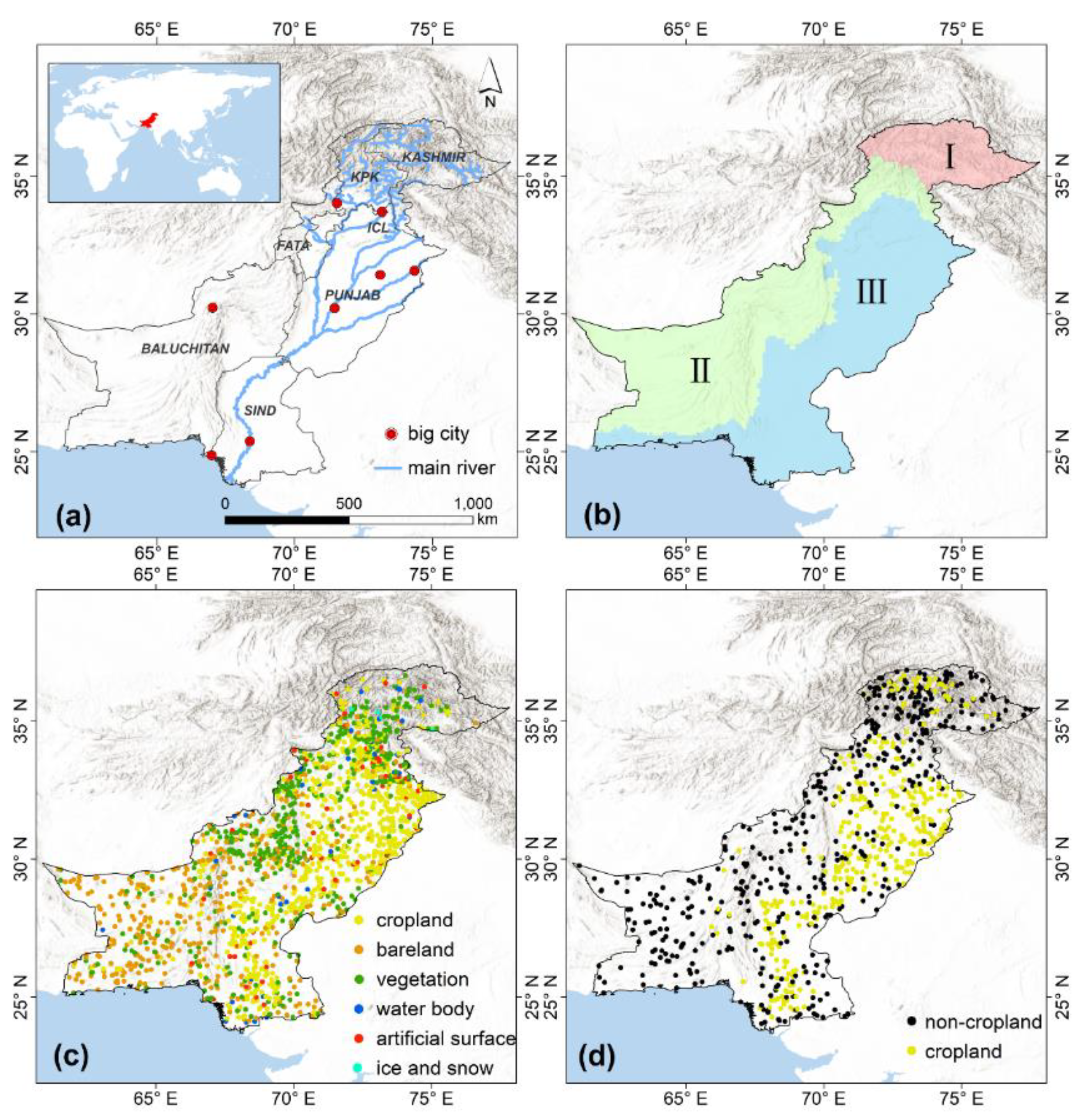
2.1. Study Area and Data Sources

Pakistan is located in a temperate zone within Southern Asia and has a total area of approximately 790,000 km2. The country has both arid and semi-arid climates, which vary in different regions (Figure 1a). In general, Pakistan has more croplands in the south and east than in the north and west. The growth of the same type of crop exhibits spatial differences in different areas [33]. The territory contains diverse terrain, including mountains (e.g., the Himalayas and Karakoram), plateaus, bare-rock areas, and deserts. As mountains, bare-rock areas, and deserts are not suitable for cultivation, cropland fields in the north and southwest are generally small in size. The southeast, which is dominated by plains, is covered by high-density cropland areas distributed along the Indus River [35].
A long history of intensive and meticulous farming in Pakistan has led to complex farming methods, a wide variety of crops, and different types of croplands adapted to different climatic and topographical conditions [39]. These factors present challenges for cropland extraction. Croplands in the southeastern plains are regularly shaped, closely arranged, and distributed over large areas. Croplands in the southwestern plateaus are scattered around cities. In addition, there are terraces in the northern mountain regions, and croplands in this region are distributed along valleys or rivers (Figure 1a). As a country that typifies Asian agriculture, Pakistan exhibits rich crop varieties, significant spatial differences in crops, intra-class variations of the same crop in different regions, and complex small-scale farming methods, including crop rotation on the same plot in different seasons and intercropping of different crops.
Based on the Google Earth Engine (GEE), 422 frames of remotely sensed Landsat-8 images were selected; these images were captured between December 2014 and January 2016. A total of 1782 training sample points and 858 test points were generated randomly using ArcGIS, and high-resolution remotely sensed images from the Google Earth were used for visual interpretations of land cover types (Table 1, Figure 1c,d and Figure 2). During the interpretation process of the remotely sensed images, vegetable gardens could not be separated from cultivated croplands; thus, the croplands extracted in this study included vegetable gardens.
In addition to remotely sensed images, this study used two additional datasets for analysis: ALOS World 3D-30, with a spatial resolution of 30 m, and 2015 WATER VAPOR-AQUA/MODIS, with a spatial resolution of 0.1° and a temporal resolution of 1 month. ALOS World 3D-30 was used to remove high mountain areas (with elevation > 3600 m and slope > 30°) that are not suitable for planting crops. WATER VAPOR-AQUA/MODIS was used to divide Pakistan into three regions according to humidity (Figure 1b) as follows: the northern mountain region (Region I, water vapor < 461 cm/year), southwestern plateau region (Region II, 461 < water vapor < 977 cm/year), and southeastern plain region (Region III, water vapor > 977 cm/year). The division of the three regions reflects the significant spatial characteristics of climate and topography in Pakistan.
Four sets of reference data were used in this study, including cropland mapping results from two different supervised classifiers (i.e., classification and regression trees (CART) and support vector machines (SVM)) and two existing global cropland datasets (i.e., Finer Resolution Observation and Monitoring of Global Land Cover (FROM-GLC) and Global Food Security Support Analysis Data (GFSAD)). The two supervised classifiers used the same training samples and remotely sensed images as ACE-DTW. The two existing global cropland datasets contained data from 2015 and had a spatial resolution of 30 m. FROM-GLC extracted croplands through multi-season remotely sensed image classifiers, and GFSAD extracted croplands through supervised time series classifiers [40,41].

2.2. Methodology

2.2.1. NDVI Time Series

The study used 422 frames of multispectral remotely sensed Landsat-8 images, which were captured between December 2014 and January 2016 (one additional month beyond estimations for improving the accuracy of time series reconstruction) and constructed a monthly NDVI time series of Pakistan for 2015. NDVI is one of the most-used vegetation indices for studying vegetation phenology [42]. The NDVI values of all the pixels were calculated, and each pixel was assigned its monthly maximum NDVI value. As a result, 14 monthly NDVI maps of Pakistan were generated. To eliminate outliers in the time series, a Savitzky–Golay (S–G) filter was used to smooth out the 14 monthly NDVI time series. The S–G filter is widely used for time series reconstruction [43,44]. It used simplified least-squares-fit convolution as its theoretical basis. After the time series were smoothed out by the S–G filter, 12 monthly NDVI maps with reconstructed time series were generated to construct a monthly time series of Pakistan croplands for 2015 (Figure 3).

2.2.2. DTW Distance

We calculated the DTW distance among the reconstructed NDVI time series of training samples. The DTW algorithm calculates the distance between two time series based on the minimum distance with the least amount of bending. The sum of the shortest path distances is called the DTW distance [45]. In this study, 12-month NDVI values of each pixel were inserted into an array as the NDVI time series of the pixel, and the DTW distance between two time series was used to characterize the similarity of two pixels. The DTW distance between two time series and the similarity between them were inversely proportional. The DTW distance is calculated as follows:
  • For Pixel Q: Qndvi = [q1, q2, …, qi, …, q12]
  • For Pixel C: Cndvi = [c1, c2, …, cj, …, c12]
DTW(Q, C) is the DTW distance between Q and C, which represents the sum of the minimum distances between each value of Qndvi and Cndvi. The cumulative distance is defined as γ(i,j), and the sequences are matched up from point (0, 0). The distance between the current point (i,j) and the initial point is d (i,j), and the minimum distance between point i on Q and point j on C is |qi—cj|. The cumulative distance γ (i,j) can be expressed as follows:
[ | q 1     c 1 | | q 1     c 2 | | q 1     c 12 | | q 2     c 1 | | q 2     c 2 | + min { γ ( 1 , 1 ) ,   γ ( 1 , 2 ) ,   γ ( 2 , 1 ) } | q 12     c 1 | | q 12     c 12 | + min { γ ( 11 , 11 ) ,   γ ( 11 , 12 ) ,   γ ( 12 , 11 ) } ]
The dynamic results obtained from the above equation are presented in matrix γ. The result of γ(12, 12) is the DTW distance between Q and C [46].

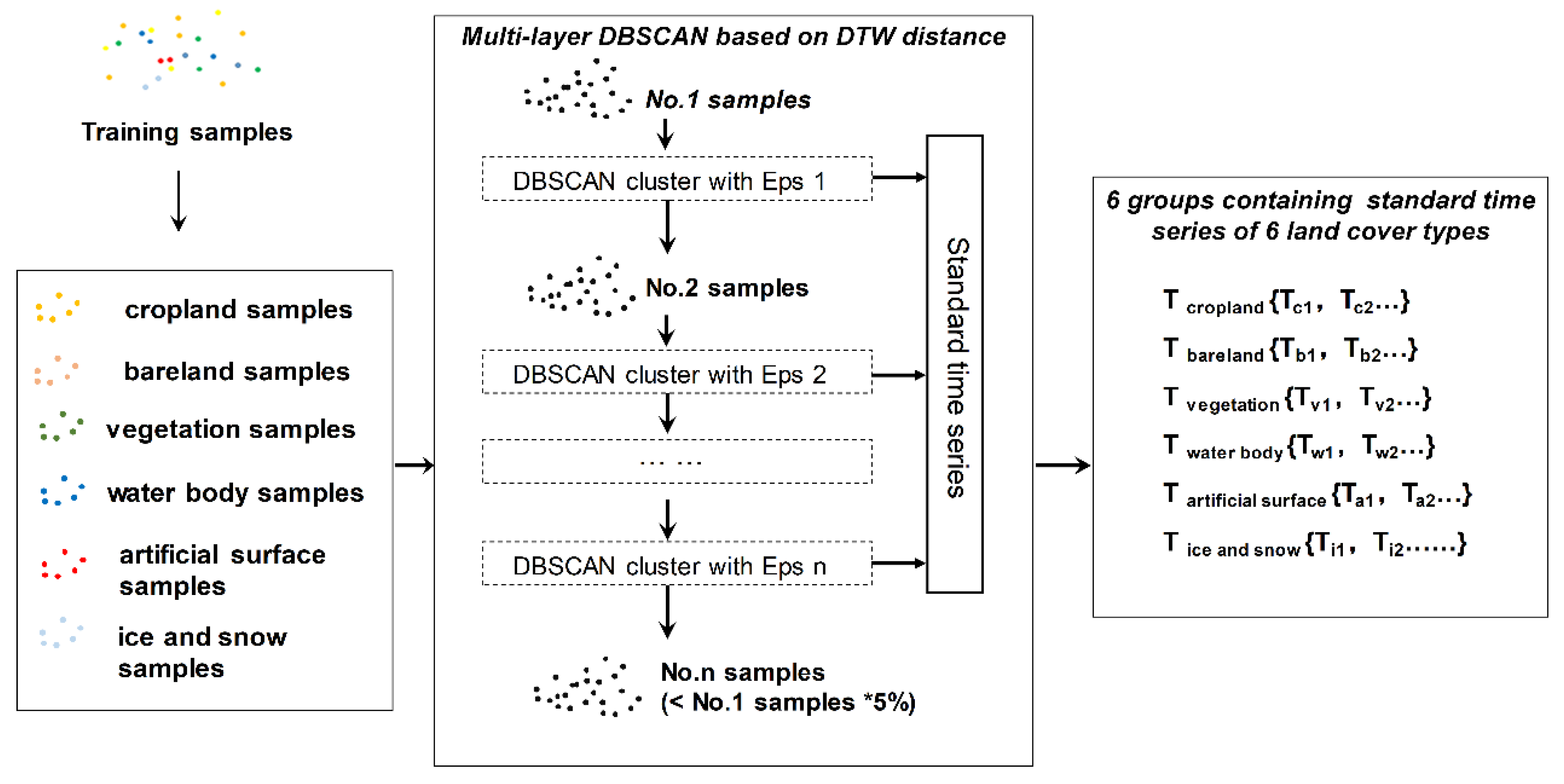
2.2.3. Multi-Layer DBSCAN

We clustered time series of training samples into different categories using a multi-layer DBSCAN based on DTW distance. Our method can ensure that more than 95% of the information obtained from NDVI describing characteristics of different land cover types is automatically captured. The DTW algorithm enables our method to avoid the subjectivity of previous methods effectively based on a priori knowledge and, thus, reduce omissions of cropland types in large areas (Figure 4).
DBSCAN is a density-based clusterer that uses the Manhattan distance as the distance between two points [47,48]. In the set of training points N, the DTW distance between the NDVI time series of two pixels (i.e., Ni and Nj) was calculated to characterize the similarity between two time series instead of using the Manhattan distance between two points. DBSCAN requires two parameters, namely, Eps and Minpts. Minpts is the minimum number of points in each category, which was set to 3 (Minpts = 3) in this study. Eps is the radius of the cluster and was obtained based on the characteristics of the set of DTW distances between training points. Specifically, the distances between all the points in the set of training points N were calculated to generate an array. The obtained array was used to produce an Eps list based on the k-means algorithm and mathematical expectations [49,50]. The first value of the list was taken as Eps for the clusterer.
The training points used in the study cover different areas in Pakistan; thus, the pairwise DTW distances between training points have a relatively large range. Consequently, a single time clusterer may produce a large number of noise points that cannot be clustered, resulting in the omission of significant amounts of useful information. To resolve this issue, a multi-layer DBSCAN was built to obtain a relatively complete time series of each type of land cover. The noise points generated by the first clusterer were used as a new point set to be reclustered. In the new round of clustering, Minpts = 3, and Eps was determined according to the new point set. If the number of noise points generated by the second clusterer was still >5% of the number of points in the original set of training points N, a new clusterer was performed until the number of noise points was <5% of the number of points in N. After the data were clustered multiple times, the typical time series of each land cover type captured >95% of the information in the training samples. Cropland categories covering relatively small areas or influenced by varying cropping methods were unlikely to be omitted. Finally, the mean value of the time series for each category was taken as the standard time series of the category.

2.2.4. Cropland Mapping

In this study, a group of standard time series were generated for six land cover types: cropland, bare land, vegetation, water body, artificial surface, and ice and snow. A group of standard time series were generated for each land cover type. The minimum DTW distance between one pixel and each standard time series in a group representing one land cover type was taken as the DTW distance between the pixel and that land cover type. The DTW distances between all pixels and all land cover types were calculated. Pixels whose DTW distance to the cropland type was smaller than that to any other land cover types were classified as cropland pixels, thereby completing the cropland mapping [32] (Figure 2). The entire mapping process was completed on the GEE, which eased the task of obtaining remotely sensed images and performing calculations for large areas (The algorithm used in this study is available on GEE at: https://code.earthengine.google.com/492035f66bf79da7a6093bf008aaa838)

2.2.5. Data Analysis

The study used 819 test samples (Figure 1, Table 1) to calculate the overall accuracies (OAs) of the cropland map produced through ACE-DTW and four referent datasets. OA (i.e., the sum of the true positives plus true negatives divided by the total number of individuals tested) is a popular measures of classification accuracy derived from a confusion matrix [51,52,53]. The accuracy calculation processes were completed on GEE (Algorithm of is available on GEE at https://code.earthengine. google.com/1cbe39a363e0cf25cf493965079d107c). ArcGIS was used for visualization of overall and detailed cropland mapping results.

3. Results

3.1. Standard Cropland Time Series in Pakistan

ACE-DTW can automatically generate standard cropland time series (Figure 5) that fully reflect the wide variety of croplands in Pakistan. After clustering the NDVI time series of cropland training points using the multi-layer DBSCAN in three regions, a total of 89 standard cropland time series were generated, including 5 for Region I, 8 for Region II, and 76 for Region III. These standard cropland time series represent the following four types of cropland: yielding one crop per year, yielding two crops per year, yielding three crops per year, and cropland with no yield or an indeterminate yield, which results in a flat curve (Figure 5). In each type, the ripening periods of different standard time series were different. For example, there were two types of crops that yield once per year with different ripening periods, i.e., from June to July (Figure 5, Curve 1) and from December to January of the following year (Figure 5, Curve 2), three types of crops that yield twice per year (Figure 5, Curves 3, 4, and 5), and two types of crops that yield thrice per year (Figure 5, Curves 6 and 7). Cropland with no yield or an indeterminate yield is represented by Curve 8.
The large number of standard cropland time series reflects the fact that Pakistan has a complicated mix of cropland types resulting from its large land area and significant regional differences in climate, topography, and farming methods [39]. This is particularly true in Region III where a total of 76 standard cropland time series were generated. To avoid omissions of cropland types, we used 89 standard cropland time series to extract croplands in three regions and map national-scale croplands in Pakistan.

3.2. Cropland Mapping Results for Pakistan

The cropland maps obtained through ACE-DTW using 89 standard cropland time series and four reference datasets (FROM-GLC, GFSAD, CART, and SVM) were relatively consistent in terms of cropland coverage in Pakistan. Cropland covered an area of approximately 2 × 10⁵ km2, of which approximately 90% was distributed in the southeastern plain region. This region has the highest cropland density in Pakistan, and the croplands in this region are mainly distributed along the Indus River. Croplands in the southwest plateau region and the northern mountain region were mainly distributed along valleys and cities, and in these two regions, croplands are small, fragmented, and discretely distributed (Figure 6). These results support previous findings regarding cropland distribution in Pakistan and similar areas [33].
To evaluate the accuracy of national-scale cropland maps, a total of 819 test samples were used to calculate OAs of five cropland maps (Figure 7). The calculations showed that ACE-DTW achieved the highest accuracy in nationwide maps compared to the reference maps. The OA of ACE-DTW was 89.7%. The commission and omission errors were 6.2% and 15.9%, respectively. The OA of ACE-DTW was higher than that of supervised classifiers for both nationwide (89.7% vs. 78.2%, 78.8%) and regional extractions (north: 93.5% vs. 89.0%, 79.8%; southeast: 88.1% vs. 68.0%, 78.8%; southwest: 93.4% vs. 81.0%, 80.1%); the OA of the nationwide extraction performed by ACE-DTW was 10% higher than that of the supervised classifiers (Figure 7). The OA of ACE-DTW was higher than the accuracies of the two existing cropland datasets in nationwide extractions (89.7% vs. 87.1%, 83.1%). At a regional level, the OA of ACE-DTW was higher than that of the two datasets in the northern mountain and southeastern plain regions (north: 93.5% vs. 87.0%, 88.5%; southeast: 88.1% vs. 83.1%, 80.8%); its accuracy was slightly lower than that of FROM-GLC but was still higher than that of GFSAD in the southwest plateau region (93.4% vs. 95.6%, 88.5%) (Figure 7). The above comparison indicates that ACE-DTW outperformed the supervised classifiers and existing global cropland maps in the 2015 national-scale cropland mapping of Pakistan.

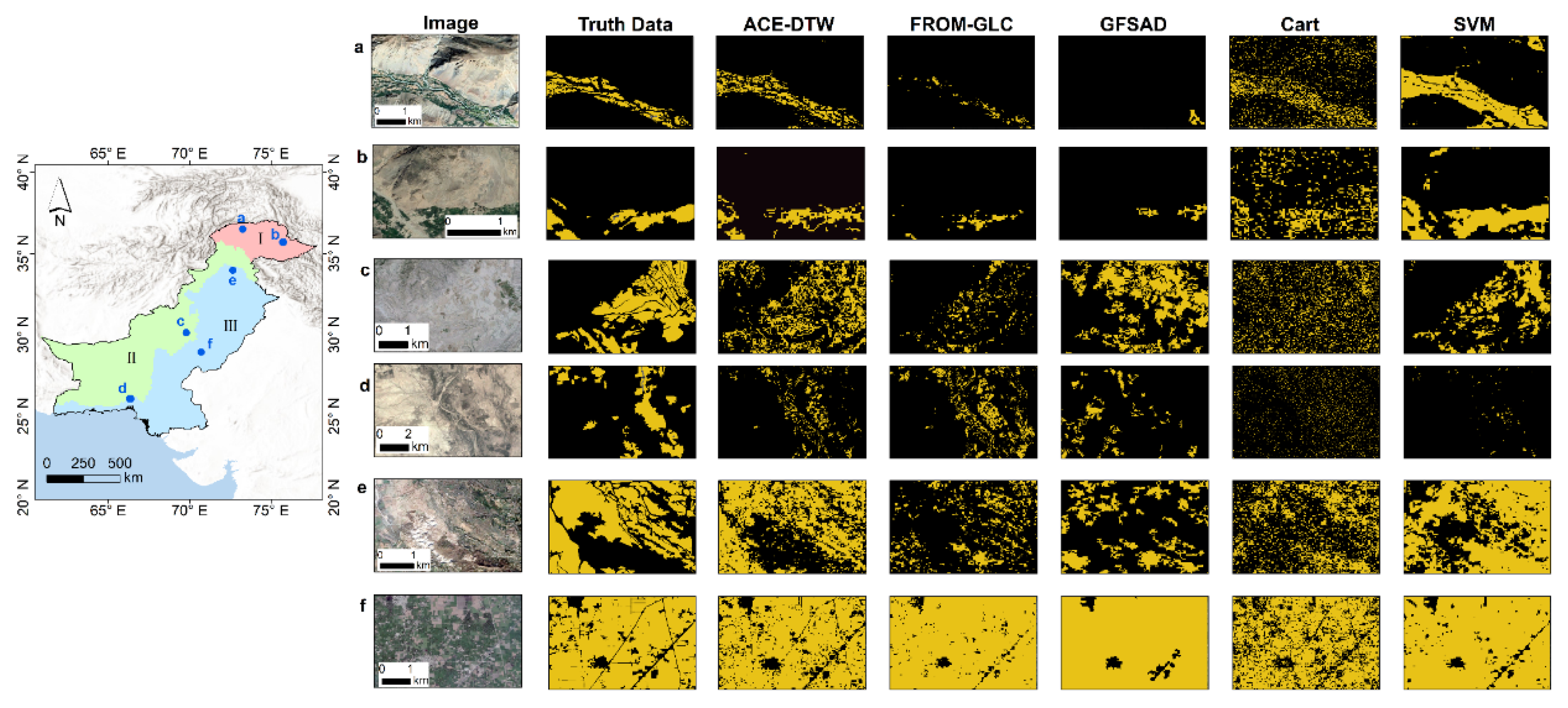
3.3. Cropland Mapping Performance in Typical Sites

Based on the overall evaluation, the performance of five cropland maps in greater detail was investigated. Six typical sites with different spatial distributions of cropland were selected for comparative analysis (Figure 8). The actual cropland coverage in these areas was plotted using Google Earth (Figure 8, Truth Data). According to the truth data, sites a and b are in the mountain region, in which the croplands are strip-shaped and distributed along the mountain valley, extending to the mountain ridges on both sides. Sites c and d are in the plateau region; the croplands in site c account for approximately half of the area, whereas croplands in site d appear to be scattered within a small area. Sites e and f are in the plain region. Site e is located at the junction of mountain and plain, which has typical croplands with proper divisions in the plains and typical narrow terraces in the mountains. Site f has the highest cropland density in Pakistan, with a cropland coverage of over 80%.
The OA results for the three regions showed that ACE-DTW performed well in mapping croplands in the mountain and plain regions (Figure 7); additionally, results exhibited in five maps of six sites showed similar high performance (Figure 8). Results in six sites showed that the supervised classifiers exhibited the worst performance among the five maps of all six sites (Figure 8, CART, SVM); thus, we do not discuss them in detail. Among the other two cropland datasets, ACE-DTW achieved higher accuracy in sites a, b, e, and f, whereas the accuracy of FROM-GLC was higher in sites c and d (Figure 8). In sites a and b, the croplands extracted by ACE-DTW were more complete, whereas the other two maps had clear omissions. Sites c and d in the southeastern plateau region mainly contain bare land and small cropland areas, and all maps for these sites exhibit errors of commissions and omissions; however, FROM-GLC best reflected the actual situation. In site f, the croplands extracted by ACE-DTW excluded the most farm roads and small cities, followed by FROM-GLC and GFSAD. For site e at the mountain-plain junction, ACE-DTW managed to remove farm roads and extract terraces more completely at the same time.
Results from six sites showed that ACE-DTW exhibited a good performance in the mountain (sites a and b) and plain regions (sites e and f). To confirm the completeness and accuracy of the standard time series of ACE-DTW in these two regions, we selected sites a and f for analysis. At mountain site a, ACE-DTW captured two types of cropland that the other two cropland maps failed to capture (Figure 9, Curves 3–4); as a result, the other two maps underestimated the area of croplands. At plain site f, where cropland density is high, ACE-DTW managed to filter out more small cities and roads because their time series are similar to those of large cities (Figure 9, Curves 12 and 9); the other two cropland maps could not differentiate these small cities and roads and croplands.

4. Discussion

ACE-DTW introduced a multi-layer DBSCAN to generate standard time series of various cropland types automatically, and, thereby, can capture cropland information at a large national scale (~790,000 km2). Although various researchers discovered the advantages of DTW in mapping croplands [4,30,31,40], existing studies primarily focused on small-scale study areas (~200–20,000 km2) [29,30,31,32] or a specific crop (e.g., rice) [4], ignoring the approaches to obtain complex standard time series at a large spatial scale. For example, Csillik et al. [32] chose two test areas: the first one is in Southern California with an area of 575 km2 and the second one is in Northwestern Texas with an area of 594 km2; Guan and Huang [4] mapped rice cropping systems in Vietnam. We used a total of 89 standard time series automatically acquired by DBSCAN for our cropland mapping in Pakistan, whereas in previous studies, only 4–16 standard time series were generally used to map croplands [4,10,31,32]. For example, Belgiu et al. [30] only used 4–5 standard time series in three study areas, and these standard time series were based on typical crops. Mondal et al. [31] used 15 standard time series in Himachal Pradesh, and these standard time series are the average of time series with similar shapes and magnitudes in 62 cropland grids. The judgment of which time series are similar was made by the researcher; hence, it is difficult to apply this method to a large area. Furthermore, by controlling the number of noise points, ACE-DTW can obtain more than 95% of the information regarding cropland samples nationwide (Figure 4). When the number of training points is increased, ACE-DTW has the potential to obtain more accurate and complete standard time series to describe the complex cropland status automatically, whereas in previous studies, to improve the ability to obtain cropland information, a greater effort was required.
ACE-DTW can extract more complete croplands in mountain region and more accurate croplands in plain region compared to the reference cropland datasets [40,41] in Pakistan (Figure 8 and Figure 9). Generally, the area of croplands in the mountain region is easily underestimated and the area of croplands in the plain region is easily overestimated [54,55]. Pflugmacher et al. [54] determined that maps tend to slightly under-predict certain small classes (croplands in mountain region in our study) and over-predict certain large classes (croplands in plain region in our study). Fritz et al. [55] found that three land cover products based on remotely sensed images missed a high proportion of cropland in the northern Sudan where the desert and the Nile Valley are located. In contrast, ACE-DTW obtained complete and accurate standard time series through multi-layer DBSCAN, to fully capture relatively complete cropland characteristics in mountain region and accurately distinguish croplands from other land cover types such as artificial surfaces in plain region. Particularly, croplands play increasingly important roles in mountain regions [56,57,58,59], and ACE-DTW can be used as an efficient method to map croplands there and might be able to help solve various problems related to ecosystem management [59], water retention and storage [60], and SDG (Sustainable Development Goal) 2 in mountain region [61].
However, ACE-DTW’s ability to distinguish croplands from sparse vegetation is limited, particularly in the plateau region of Pakistan (Figure 6, Figure 7 and Figure 8). Such misidentifications often occur in remote sensing-based cropland mapping studies [33,59,62,63,64]. For example, Matton et al. [63] found that croplands are easily mixed with neighboring vegetation in fields lacking cropland management. Nabil et al. [64] found that spectral similarity with grasslands and other herbaceous vegetation limits accurate mapping of African cropland, especially in arid and semi-arid areas. In these study areas that are similar to the plateau region of Pakistan, the rainfall regime causes synchronized phenology between crops and natural vegetation; croplands which are fallow in the dry season and cultivated again in the rainy season [65] are spectrally similar to natural vegetation that withers in the dry season and grows in the rainy season [66] in NDVI time series; hence, it is difficult to separate crops from natural vegetation. Addressing this problem is a challenge and requires further investigation. In future studies, additional remotely sensed images-based indexes (e.g., the enhanced vegetation index of multispectral remotely sensed images [67] and the C-band like-polarized ratio of synthetic aperture radar images [12]) and the fusion of multi-source data (e.g., Landsat-7, Landsat-8, and MODIS [68]) can be integrated in our ACE-DTW algorithm or other DTW-based algorithms to better distinguish croplands with sparse vegetation.

5. Conclusions

In this study, we combined the DTW algorithm and DBSCAN to develop a new method (ACE-DTW) to map croplands with high accuracy. The major advantage of ACE-DTW is that it can automatically obtain standard time series based on the pairwise DTW distances between training samples. Using ACE-DTW, we mapped croplands on a national scale in Pakistan, a country that typifies Asian agriculture with many cropland types, a long history of intensive and meticulous farming, and complex crop growth patterns. Our results showed that ACE-DTW significantly improved the accuracy of cropland mapping compared to conventional supervised classifiers and existing global cropland datasets. In particular, ACE-DTW can map complete croplands in mountain regions because it captures comprehensive time series of mountain croplands, while small and fragmented croplands in mountain regions are typically ignored or underestimated in existing cropland studies, which is problematic as this kind of cropland accounts for a large proportion of the total cropland area. To summarize, ACE-DTW provides an approach for complete and accurate national cropland mapping, which has great potential to help ensure food security and achieve SDG 2, particularly in countries that lack agricultural modernization.

Author Contributions

Conceptualization, Z.G., K.Y.; methodology, Z.G., K.Y., C.L.; validation, Z.G., K.Y.; data curation, Z.G., K.Y., X.L.; writing—original draft preparation, Z.G.; writing—review and editing, Z.G., K.Y.; visualization, Z.G., K.Y., X.L., C.L.; supervision, K.Y.; project administration, K.Y.; funding acquisition, K.Y., L.C., M.L. All authors have read and agreed to the published version of the manuscript.

Funding

This work was supported by the National Key R&D Program of China (2017YFB0504205), the National Natural Science Foundation of China (41871327), and the Fundamental Research Funds for the Central Universities (14380070).

Acknowledgments

The authors are grateful to the United States Geological Survey for providing Landsat-8 images, to Google Earth for providing high-resolution remotely sensed images, and to Google Earth Engine for providing the image processing environment.

Conflicts of Interest

The authors declare no conflict of interest.

References

  1. Useya, J.; Chen, S. Exploring the Potential of Mapping Cropping Patterns on Smallholder Scale Croplands Using Sentinel-1 SAR Data. Chin. Geogr. Sci. 2019, 29, 626–639. [Google Scholar] [CrossRef] [Green Version]
  2. Wallace, C.S.A.; Thenkabail, P.; Rodriguez, J.R.; Brown, M.K. Fallow-land Algorithm based on Neighborhood and Temporal Anomalies (FANTA) to map planted versus fallowed croplands using MODIS data to assist in drought studies leading to water and food security assessments. GISci. Remote Sens. 2017, 54, 258–282. [Google Scholar] [CrossRef] [Green Version]
  3. Tasumi, M.; Allen, R.G. Satellite-based ET mapping to assess variation in ET with timing of crop development. Agric. Water Manag. 2007, 88, 54–62. [Google Scholar] [CrossRef]
  4. Guan, X.; Huang, C.; Liu, G.; Meng, X.; Liu, Q. Mapping Rice Cropping Systems in Vietnam Using an NDVI-Based Time-Series Similarity Measurement Based on DTW Distance. Remote Sens. 2016, 8, 19. [Google Scholar] [CrossRef] [Green Version]
  5. Phalke, A.R.; Özdoğan, M. Large area cropland extent mapping with Landsat data and a generalized classifier. Remote Sens. Environ. 2018, 219, 180–195. [Google Scholar] [CrossRef]
  6. Teluguntla, P.; Thenkabail, P.S.; Xiong, J.; Gumma, M.K.; Congalton, R.G.; Oliphant, A.; Poehnelt, J.; Yadav, K.; Rao, M.; Massey, R. Spectral matching techniques (SMTs) and automated cropland classification algorithms (ACCAs) for mapping croplands of Australia using MODIS 250-m time-series (2000–2015) data. Int. J. Digit. Earth 2017, 10, 944–977. [Google Scholar] [CrossRef] [Green Version]
  7. Waldner, F.; De Abelleyra, D.; Verón, S.R.; Zhang, M.; Wu, B.; Plotnikov, D.; Bartalev, S.; Lavreniuk, M.S.; Skakun, S.; Kussul, N.; et al. Towards a set of agrosystem-specific cropland mapping methods to address the global cropland diversity. Int. J. Remote Sens. 2016, 37, 3196–3231. [Google Scholar] [CrossRef] [Green Version]
  8. Dong, J.; Xiao, X.; Zhang, G.; Menarguez, M.A.; Choi, C.Y.; Qin, Y.; Luo, P.; Zhang, Y.; Moore, B. Northward expansion of paddy rice in northeastern Asia during 2000–2014. Geophys. Res. Lett. 2016, 43, 3754–3761. [Google Scholar] [CrossRef] [Green Version]
  9. Ragettli, S.; Herberz, T.; Siegfried, T. An Unsupervised Classification Algorithm for Multi-Temporal Irrigated Area Mapping in Central Asia. Remote Sens. 2018, 10, 1823. [Google Scholar] [CrossRef] [Green Version]
  10. Minasny, B.; Shah, R.M.; Soh, N.C.; Arif, C.; Setiawan, B.I. Automated Near-Real-Time Mapping and Monitoring of Rice Extent, Cropping Patterns, and Growth Stages in Southeast Asia Using Sentinel-1 Time Series on a Google Earth Engine Platform. Remote Sens. 2019, 11, 1666. [Google Scholar] [CrossRef] [Green Version]
  11. Forkuor, G.; Conrad, C.; Thiel, M.; Zoungrana, B.J.-B.; Tondoh, J.E. Multiscale Remote Sensing to Map the Spatial Distribution and Extent of Cropland in the Sudanian Savanna of West Africa. Remote Sens. 2017, 9, 839. [Google Scholar] [CrossRef] [Green Version]
  12. Nguyen, D.B.; Wagner, W. European Rice Cropland Mapping with Sentinel-1 Data: The Mediterranean Region Case Study. Water 2017, 9, 392. [Google Scholar] [CrossRef]
  13. Hao, P.-Y.; Löw, F.; Biradar, C. Annual Cropland Mapping Using Reference Landsat Time Series—A Case Study in Central Asia. Remote Sens. 2018, 10, 2057. [Google Scholar] [CrossRef] [Green Version]
  14. Gómez, C.; White, J.C.; Wulder, M.A. Optical remotely sensed time series data for land cover classification: A review. ISPRS J. Photogramm. Remote Sens. 2016, 116, 55–72. [Google Scholar] [CrossRef] [Green Version]
  15. Hackman, K.O.; Gong, P.; Wang, J. New land-cover maps of Ghana for 2015 using Landsat 8 and three popular classifiers for biodiversity assessment. Int. J. Remote Sens. 2017, 38, 4008–4021. [Google Scholar] [CrossRef]
  16. Makhamreh, Z. Derivation of vegetation density and land-use type pattern in mountain regions of Jordan using multi-seasonal SPOT images. Environ. Earth Sci. 2018, 77, 384. [Google Scholar] [CrossRef]
  17. Yamamoto, Y.; Oberthür, T.; Lefroy, R. Spatial identification by satellite imagery of the crop–fallow rotation cycle in northern Laos. Environ. Dev. Sustain. 2007, 11, 639–654. [Google Scholar] [CrossRef]
  18. Zhu, C.; Lu, D.; Victoria, D.D.C.; Dutra, L.V. Mapping Fractional Cropland Distribution in Mato Grosso, Brazil Using Time Series MODIS Enhanced Vegetation Index and Landsat Thematic Mapper Data. Remote Sens. 2016, 8, 22. [Google Scholar] [CrossRef] [Green Version]
  19. Liu, L.; Xiao, X.; Qin, Y.; Wang, J.; Xu, X.; Hu, Y.; Qiao, Z. Mapping cropping intensity in China using time series Landsat and Sentinel-2 images and Google Earth Engine. Remote Sens. Environ. 2020, 239, 111624. [Google Scholar] [CrossRef]
  20. Bellón, B.; Bégué, A.; Seen, D.L.; De Almeida, C.A.; Simões, M. A Remote Sensing Approach for Regional-Scale Mapping of Agricultural Land-Use Systems Based on NDVI Time Series. Remote Sens. 2017, 9, 600. [Google Scholar] [CrossRef] [Green Version]
  21. Fan, C.; Zheng, B.; Myint, S.W.; Aggarwal, R. Characterizing changes in cropping patterns using sequential Landsat imagery: An adaptive threshold approach and application to Phoenix, Arizona. Int. J. Remote Sens. 2014, 35, 7263–7278. [Google Scholar] [CrossRef]
  22. Tiwari, V.; Matin, M.A.; Qamer, F.M.; Ellenburg, W.L.; Bajracharya, B.; Vadrevu, K.; Rushi, B.R.; Yusafi, W. Wheat Area Mapping in Afghanistan Based on Optical and SAR Time-Series Images in Google Earth Engine Cloud Environment. Front. Environ. Sci. 2020, 8, 77. [Google Scholar] [CrossRef]
  23. Xiong, J.; Thenkabail, P.S.; Tilton, J.C.; Gumma, M.K.; Teluguntla, P.; Oliphant, A.; Congalton, R.G.; Yadav, K.; Gorelick, N. Nominal 30-m Cropland Extent Map of Continental Africa by Integrating Pixel-Based and Object-Based Algorithms Using Sentinel-2 and Landsat-8 Data on Google Earth Engine. Remote Sens. 2017, 9, 1065. [Google Scholar] [CrossRef] [Green Version]
  24. Chen, Y.; Lu, D.; Moran, E.; Batistella, M.; Dutra, L.V.; Sanches, I.D.; Da Silva, R.F.B.; Huang, J.; Luiz, A.J.B.; De Oliveira, M.A.F. Mapping croplands, cropping patterns, and crop types using MODIS time-series data. Int. J. Appl. Earth Obs. Geoinf. 2018, 69, 133–147. [Google Scholar] [CrossRef]
  25. Ma, L.; Yang, S.; Gu, Q.; Li, J.; Yang, X.; Wang, J.; Ding, J. Spatial and temporal mapping of cropland expansion in northwestern China with multisource remotely sensed data. Catena 2019, 183, 104192. [Google Scholar] [CrossRef]
  26. Li, Z.; Fox, J.M. Mapping rubber tree growth in mainland Southeast Asia using time-series MODIS 250 m NDVI and statistical data. Appl. Geogr. 2012, 32, 420–432. [Google Scholar] [CrossRef]
  27. Wu, Z.; Thenkabail, P.S.; Mueller, R.; Zakzeski, A.; Melton, F.; Johnson, L.; Rosevelt, C.; Dwyer, J.; Jones, J.; Verdin, J.P. Seasonal cultivated and fallow cropland mapping using MODIS-based automated cropland classification algorithm. J. Appl. Remote Sens. 2014, 8, 083685. [Google Scholar] [CrossRef] [Green Version]
  28. Kamir, E.; Waldner, F.; Hochman, Z. Estimating wheat yields in Australia using climate records, satellite image time series and machine learning methods. ISPRS J. Photogramm. Remote Sens. 2020, 160, 124–135. [Google Scholar] [CrossRef]
  29. Guan, X.; Liu, G.; Huang, C.; Meng, X.; Liu, Q.; Wu, C.; Ablat, X.; Chen, Z.; Wang, Q. An Open-Boundary Locally Weighted Dynamic Time Warping Method for Cropland Mapping. ISPRS Int. J. Geoinf. 2018, 7, 75. [Google Scholar] [CrossRef] [Green Version]
  30. Belgiu, M.; Csillik, O. Sentinel-2 cropland mapping using pixel-based and object-based time-weighted dynamic time warping analysis. Remote Sens. Environ. 2018, 204, 509–523. [Google Scholar] [CrossRef]
  31. Mondal, S.; Jeganathan, C. Mountain agriculture extraction from time-series MODIS NDVI using dynamic time warping technique. Int. J. Remote Sens. 2018, 39, 3679–3704. [Google Scholar] [CrossRef]
  32. Csillik, O.; Belgiu, M.; Asner, G.P.; Kelly, M. Object-Based Time-Constrained Dynamic Time Warping Classification of Crops Using Sentinel-2. Remote Sens. 2019, 11, 1257. [Google Scholar] [CrossRef] [Green Version]
  33. Gumma, M.K.; Thenkabail, P.S.; Teluguntla, P.G.; Oliphant, A.; Xiong, J.; Giri, C.; Pyla, V.; Dixit, S.; Whitbread, A.M. Agricultural cropland extent and areas of South Asia derived using Landsat satellite 30-m time-series big-data using random forest machine learning algorithms on the Google Earth Engine cloud. GIScience Remote Sens. 2019, 57, 302–322. [Google Scholar] [CrossRef] [Green Version]
  34. Anser, M.K.; Hina, T.; Hameed, S.; Nasir, M.H.; Ahmed, I.; Naseer, M.A.U.R. Modeling Adaptation Strategies against Climate Change Impacts in Integrated Rice-Wheat Agricultural Production System of Pakistan. Int. J. Environ. Res. Public Health 2020, 17, 2522. [Google Scholar] [CrossRef] [Green Version]
  35. Gumma, M.K.; Thenkabail, P.S.; Teluguntla, P.; Rao, M.N.; Mohammed, I.A.; Whitbread, A.M. Mapping rice-fallow cropland areas for short-season grain legumes intensification in South Asia using MODIS 250 m time-series data. Int. J. Digit. Earth 2016, 9, 981–1003. [Google Scholar] [CrossRef] [Green Version]
  36. Oliphant, A.J.; Thenkabail, P.S.; Teluguntla, P.; Xiong, J.; Gumma, M.K.; Congalton, R.G.; Yadav, K. Mapping cropland extent of Southeast and Northeast Asia using multi-year time-series Landsat 30-m data using a random forest classifier on the Google Earth Engine Cloud. Int. J. Appl. Earth Obs. Geoinf. 2019, 81, 110–124. [Google Scholar] [CrossRef]
  37. Jat, M.L.; Chakraborty, D.; Ladha, J.K.; Rana, D.S.; Gathala, M.K.; McDonald, A.; Gerard, B. Conservation agriculture for sustainable intensification in South Asia. Nat. Sustain. 2020, 3, 336–343. [Google Scholar] [CrossRef]
  38. Spengler, R.N., II; Ryabogina, N.; Tarasov, P.E.; Wagner, M. The spread of agriculture into northern Central Asia: Timing, pathways, and environmental feedbacks. Holocene 2016, 26, 1527–1540. [Google Scholar] [CrossRef]
  39. Gathala, M.K.; Timsina, J.; Islam, M.S.; Krupnik, T.J.; Bose, T.R.; Islam, N.; Rahman, M.M.; Hossain, M.I.; Harun-Ar-Rashid, M.; Ghosh, A.K.; et al. Productivity, profitability, and energetics: A multi-criteria assessment of farmers’ tillage and crop establishment options for maize in intensively cultivated environments of South Asia. Field Crop. Res. 2016, 186, 32–46. [Google Scholar] [CrossRef]
  40. Yadav, K.; Congalton, R.G. Accuracy Assessment of Global Food Security-Support Analysis Data (GFSAD) Cropland Extent Maps Produced at Three Different Spatial Resolutions. Remote Sens. 2019, 11, 630. [Google Scholar] [CrossRef] [Green Version]
  41. Gong, P.; Liu, H.; Zhang, M.; Li, C.; Wang, J.; Huang, H.; Clinton, N.; Ji, L.; Li, W.; Bai, Y.; et al. Stable classification with limited sample: Transferring a 30-m resolution sample set collected in 2015 to mapping 10-m resolution global land cover in 2017. Sci. Bull. 2019, 64, 370–373. [Google Scholar] [CrossRef] [Green Version]
  42. Yan, L.; Roy, D.P. Automated crop field extraction from multi-temporal Web Enabled Landsat Data. Remote Sens. Environ. 2014, 144, 42–64. [Google Scholar] [CrossRef] [Green Version]
  43. Savitzky, A.; Golay, M.J.E. Smoothing and Differentiation of Data by Simplified Least Squares Procedures. Anal. Chem. 1964, 36, 1627–1639. [Google Scholar] [CrossRef]
  44. Chen, J.; Jönsson, P.; Tamura, M.; Gu, Z.H.; Matsushita, B.; Eklundh, L. A simple method for reconstructing a high-quality NDVI time-series data set based on the Savitzky–Golay filter. Remote Sens. Environ. 2004, 91, 332–344. [Google Scholar] [CrossRef]
  45. Sakoe, H.; Chiba, S. Dynamic programming algorithm optimization for spoken word recognition. IEEE Trans. Acoust. Speech Signal Process. 1978, 26, 43–49. [Google Scholar] [CrossRef] [Green Version]
  46. Yan, J.; Wang, L.; Song, W.; Chen, Y.; Chen, X.; Deng, Z. A time-series classification approach based on change detection for rapid land cover mapping. ISPRS J. Photogramm. Remote Sens. 2019, 158, 249–262. [Google Scholar] [CrossRef]
  47. Schubert, E.; Sander, J.; Ester, M.; Kriegel, H.P.; Xu, X. DBSCAN Revisited, Revisited: Why and How You Should (Still) Use DBSCAN. ACM Trans. Database Syst. 2017, 42, 1–21. [Google Scholar] [CrossRef]
  48. Ester, M.; Kriegel, H.P.; Sander, J.; Xu, X. A Density-Based Algorithm for Discovering Clusters in Large Spatial Databases with Noise. In Proceedings of the 2nd International Conference on Knowledge Discovery and Data Mining KDD-96, Portland, OR, USA, 2–4 August 1996; pp. 226–231. [Google Scholar]
  49. Chang, C.-C.; Lin, C.-J. LIBSVM: A library for support vector machines. ACM Trans. Intell. Syst. Technol. 2011, 2, 1–27. [Google Scholar] [CrossRef]
  50. Guyon, I.; Weston, J.; Barnhill, S.; Vapnik, V. Gene Selection for Cancer Classification using Support Vector Machines. Mach. Learn. 2002, 46, 389–422. [Google Scholar] [CrossRef]
  51. Foody, G.M. Status of land cover classification accuracy assessment. Remote Sens. Environ. 2002, 80, 185–201. [Google Scholar] [CrossRef]
  52. Stein, A.; Aryal, J.; Gort, G. Use of the Bradley-Terry model to quantify association in remotely sensed images. IEEE Trans. Geosci. Remote Sens. 2005, 43, 852–856. [Google Scholar] [CrossRef]
  53. Alberg, A.J.; Park, J.W.; Hager, B.W.; Brock, M.V.; Diener-West, M. The use of “overall accuracy” to evaluate the validity of screening or diagnostic tests. J. Gen. Intern. Med. 2004, 19, 460–465. [Google Scholar] [CrossRef] [Green Version]
  54. Pflugmacher, D.; Rabe, A.; Peters, M.; Hostert, P. Mapping pan-European land cover using Landsat spectral-temporal metrics and the European LUCAS survey. Remote Sens. Environ. 2019, 221, 583–595. [Google Scholar] [CrossRef]
  55. Fritz, S.; See, L.; Rembold, F. Comparison of global and regional land cover maps with statistical information for the agricultural domain in Africa. Int. J. Remote Sens. 2010, 31, 2237–2256. [Google Scholar] [CrossRef]
  56. Choenkwan, S.; Fox, J.M.; Rambo, A.T. Agriculture in the Mountains of Northeastern Thailand: Current Situation and Prospects for Development. Mt. Res. Dev. 2014, 34, 95–106. [Google Scholar] [CrossRef]
  57. Adhikari, L.; Hussain, A.; Rasul, G. Tapping the Potential of Neglected and Underutilized Food Crops for Sustainable Nutrition Security in the Mountains of Pakistan and Nepal. Sustainability 2017, 9, 291. [Google Scholar] [CrossRef] [Green Version]
  58. Liang, L.; Gong, P. Evaluation of global land cover maps for cropland area estimation in the conterminous United States. Int. J. Digit. Earth 2015, 8, 102–117. [Google Scholar] [CrossRef]
  59. Tovar, C.; Seijmonsbergen, A.C.; Duivenvoorden, J.F. Monitoring land use and land cover change in mountain regions: An example in the Jalca grasslands of the Peruvian Andes. Landsc. Urban Plan. 2013, 112, 40–49. [Google Scholar] [CrossRef]
  60. Luo, L.; Li, F.; Dai, Z.; Yang, X.; Liu, W.; Fang, X. Terrace extraction based on remote sensing images and digital elevation model in the loess plateau, China. Earth Sci. Inform. 2020, 13, 433–446. [Google Scholar] [CrossRef]
  61. Liu, L.; Liang, Y.; Hashimoto, S. Integrated assessment of land-use/coverage changes and their impacts on ecosystem services in Gansu Province, northwest China: Implications for sustainable development goals. Sustain. Sci. 2020, 15, 297–314. [Google Scholar] [CrossRef]
  62. Gong, P.; Wang, J.; Yu, L.; Zhao, Y.; Zhao, Y.; Liang, L.; Niu, Z.; Huang, X.; Fu, H.; Liu, S.; et al. Finer resolution observation and monitoring of global land cover: First mapping results with Landsat TM and ETM+ data. Int. J. Remote Sens. 2013, 34, 2607–2654. [Google Scholar] [CrossRef] [Green Version]
  63. Matton, N.; Canto, G.S.; Waldner, F.; Valero, S.; Morin, D.; Inglada, J.; Arias, M.; Bontemps, S.; Koetz, B.; Defourny, P. An Automated Method for Annual Cropland Mapping along the Season for Various Globally-Distributed Agrosystems Using High Spatial and Temporal Resolution Time Series. Remote Sens. 2015, 7, 13208–13232. [Google Scholar] [CrossRef] [Green Version]
  64. Nabil, M.; Zhang, M.; Bofana, J.; Wu, B.; Stein, A.; Dong, T.; Zeng, H.; Shang, J. Assessing factors impacting the spatial discrepancy of remote sensing based cropland products: A case study in Africa. Int. J. Appl. Earth Obs. Geoinf. 2020, 85, 102010. [Google Scholar] [CrossRef]
  65. Conrad, C.; Lamers, J.P.A.; Ibragimov, N.; Löw, F.; Martius, C. Analysing irrigated crop rotation patterns in arid Uzbekistan by the means of remote sensing: A case study on post-Soviet agricultural land use. J. Arid. Environ. 2016, 124, 150–159. [Google Scholar] [CrossRef]
  66. Gong, P.; Yu, L.; Li, C.; Wang, J.; Liang, L.; Li, X.; Ji, L.; Bai, Y.; Cheng, Y.; Zhu, Z. A new research paradigm for global land cover mapping. Ann. GIS 2016, 22, 87–102. [Google Scholar] [CrossRef] [Green Version]
  67. Wang, L.H.; Qi, F.; Shen, X.; Huang, J.L. Monitoring Multiple Cropping Index of Henan Province, China Based on MODIS-EVI Time Series Data and Savitzky-Golay Filtering Algorithm. Comput. Model. Eng. Sci. 2019, 119, 331–348. [Google Scholar] [CrossRef] [Green Version]
  68. Ding, M.; Guan, Q.; Li, L.; Zhang, H.; Liu, C.; Zhang, L. Phenology-Based Rice Paddy Mapping Using Multi-Source Satellite Imagery and a Fusion Algorithm Applied to the Poyang Lake Plain, Southern China. Remote Sens. 2020, 12, 1022. [Google Scholar] [CrossRef] [Green Version]
Figure 1. Study area and data sources. (a) Map of Pakistan; (b) Three humidity regions of Pakistan. (c) Training samples (n = 1782), and (d) Test samples (n = 858) for cropland mapping.
Remotesensing 12 03644 g001
Figure 2. Cropland mapping using the automatic cropland extraction method based on the DTW algorithm and DBSCAN (ACE-DTW). Normalized difference vegetation index (NDVI) time series are first built from multi-temporal Landsat-8 images. Dynamic time warping (DTW) and density-based spatial clustering of applications with noise (DBSCAN) are then used to create a standard time series of six land cover types and to distinguish cropland from the other land cover types. Cropland maps derived from support vector machines (SVM) and classification and regression trees (CART) supervised classifiers and two existing global cropland datasets are used as reference datasets to evaluate cropland mapping accuracy.
Remotesensing 12 03644 g002
Figure 3. Example site of NDVI time series reconstruction using an S–G filter. Multi-temporal Landsat-8 images between December 2014 and January 2016 are used to build 14 monthly NDVI maps. These maps are then used to generate 12 monthly NDVI maps with time series reconstruction based on the S–G filter.
Remotesensing 12 03644 g003
Figure 4. Multi-layer DBSCAN based on DTW distance to obtain standard time series of six land cover types. All the training samples (No. 1 samples) are used as inputs for the first DBSCAN cluster with Eps 1 (the first cluster’s radius determined according to the No. 1 samples), and the output noise points are used as No. 2 samples to be reclustered. Eps 2 is determined according to the No. 2 samples. New clusters are built iteratively until the number of noise points is less than 5% that of the No. 1 samples, thereby ensuring that the standard time series of each land cover type captures more than 95% of the information of all the training samples.
Remotesensing 12 03644 g004
Figure 5. Some representative standard time series for croplands in Pakistan. Curves 1–2 represent croplands yielding one crop per year, curves 3–5 represent croplands yielding two crops per year, curves 6–7 represent croplands yielding three crops per year, and curve 8 represents croplands with no yield or an indeterminate yield.
Remotesensing 12 03644 g005
Figure 6. (a) Cropland training samples (n = 747) and cropland maps derived from (b) ACE-DTW, (c) Finer Resolution Observation and Monitoring of Global Land Cover (FROM-GLC-2015), (d) Global Food Security Support Analysis Data (GFSAD), (e) CART, and (f) SVM.
Remotesensing 12 03644 g006
Figure 7. Cropland mapping accuracy in Pakistan (as a whole) and the three humidity regions. The overall accuracy of ACE-DTW is higher than that of reference maps in Pakistan, the northern mountain region (Region I), and southeastern plain regions (Region II), but is slightly lower than that of FROM-GLC in the southwestern plateau region (Region III).
Remotesensing 12 03644 g007
Figure 8. Cropland mapping results in six typical cropland spatial distributions sites. ACE-DTW performs best in sites (a) and (b) in the mountain region (region I) and sites (e) and (f) in the plain region (region II) but exhibits misclassification with sparse vegetation in sites (c) and (d) in the plateau region (region III).
Remotesensing 12 03644 g008
Figure 9. Time series of typical points in sites a and f of Figure 8 to present the completeness and accuracy of the standard time series of ACE-DTW. ACE-DTW captures more cropland types (Curves 3–4) in the mountain region (region I) and distinguishes croplands and small cities according to the similarity of NDVI time series between small cities and large cities in the plain region (region III) (Curves 9 and 12).
Remotesensing 12 03644 g009
Table 1. Number of samples for visual interpretation
Land Cover TypesCroplandBarelandVegetationWater BodyArtificial SurfaceIce and SnowTotal
Training samples747445476416851782
Test samples371487858
Publisher’s Note: MDPI stays neutral with regard to jurisdictional claims in published maps and institutional affiliations.

