Application of Multiple Geomatic Techniques for Coastline Retreat Analysis: The Case of Gerra Beach (Cantabrian Coast, Spain)

 ,
,  , ,
, ,
Abstract
:
1. Introduction
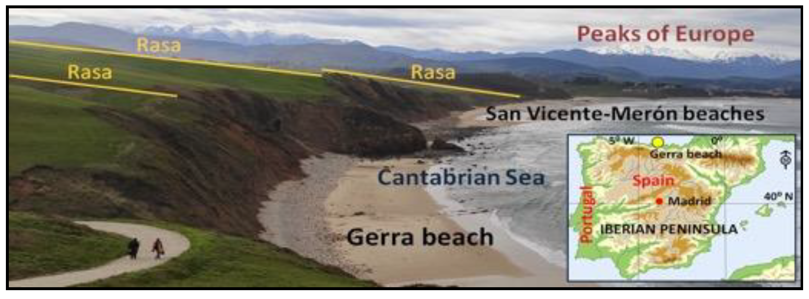
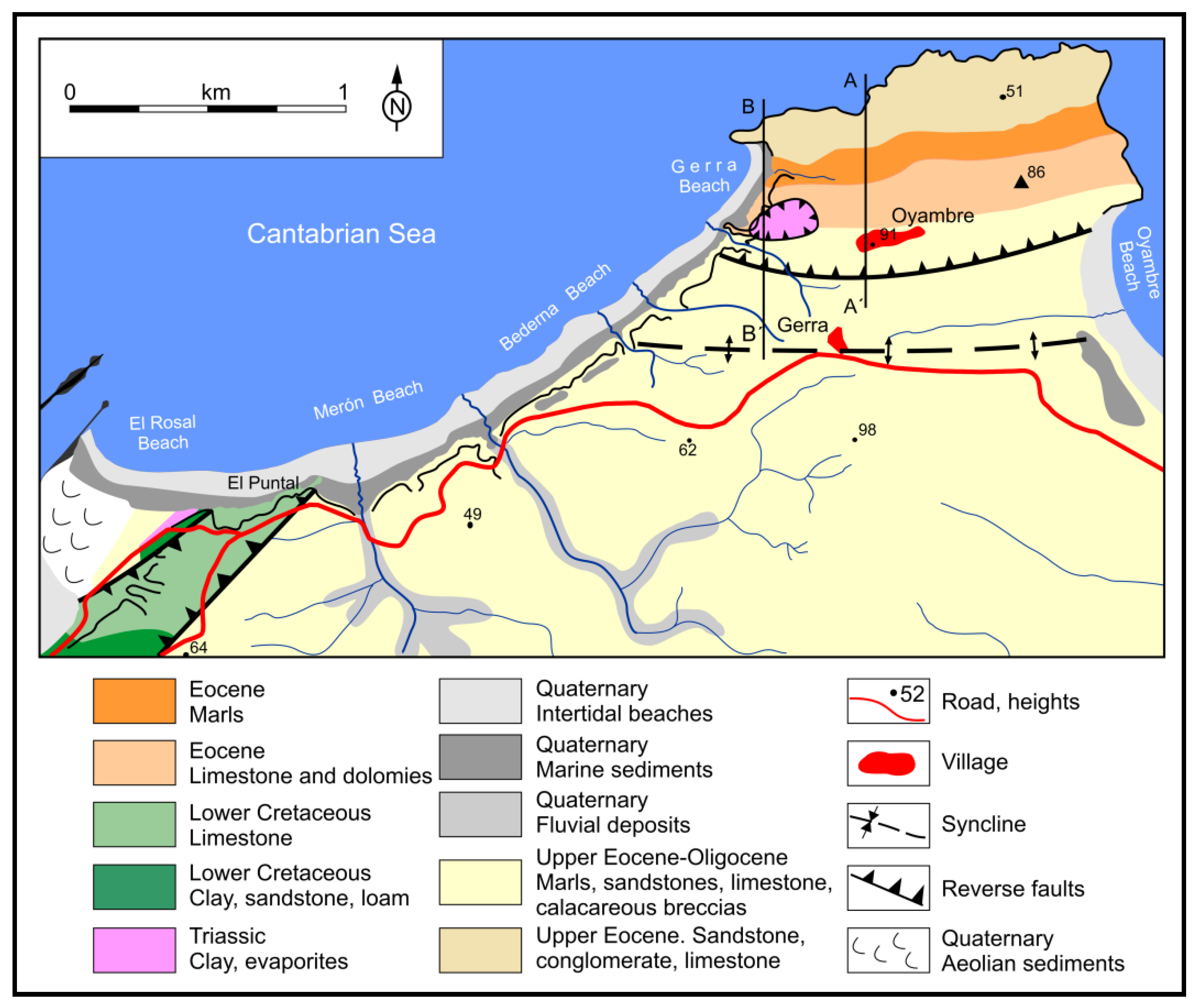
2. The Study Area
3. Data Acquisition and Methodology
3.1. Aerial Acquired Data (1956–2018)
3.2. Terrestrial Laser Scanning Data (2012–2020)
3.3. Analysis Evolution of the Beach and Coastline on the Top and Toe of the Cliff
4. Results
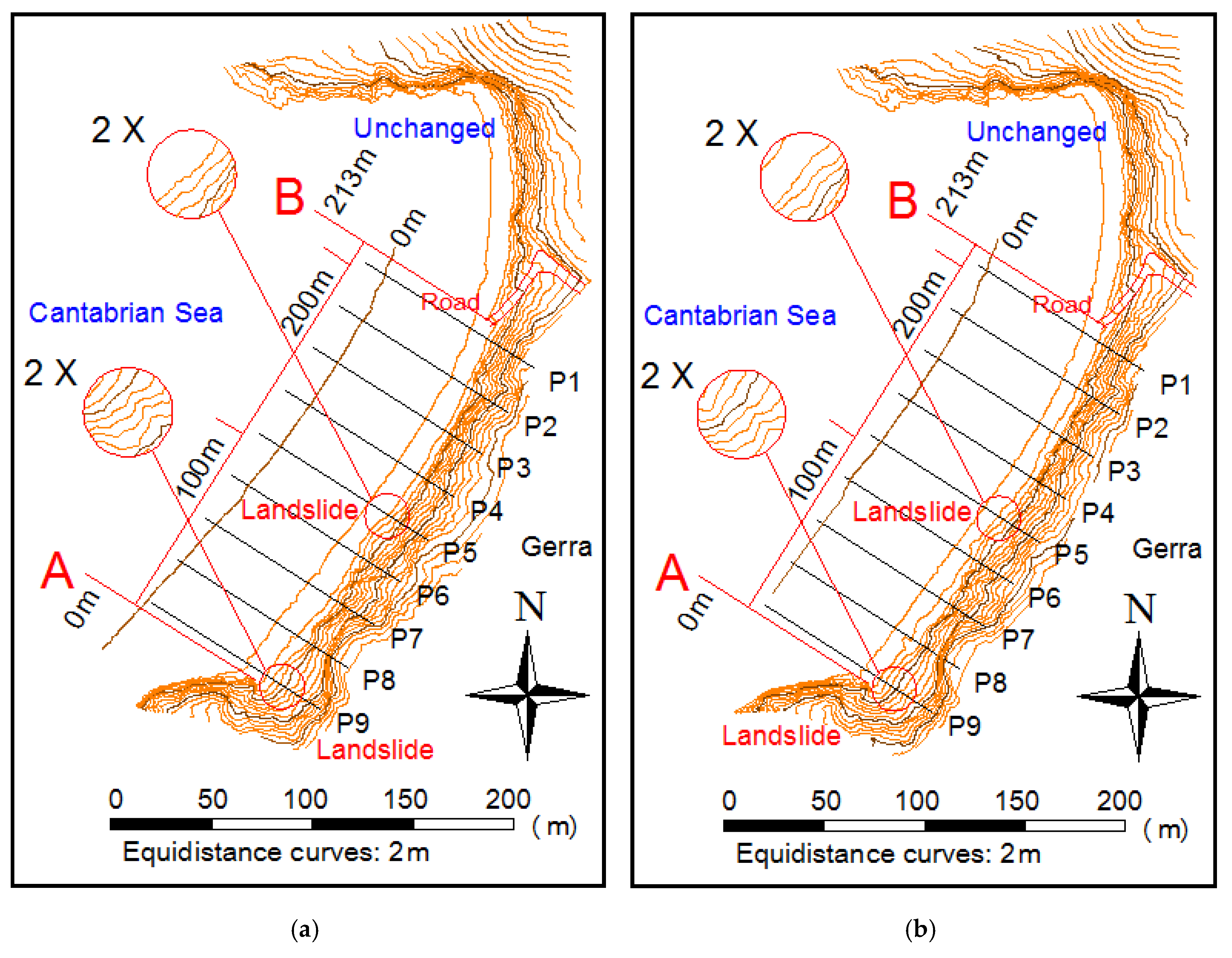
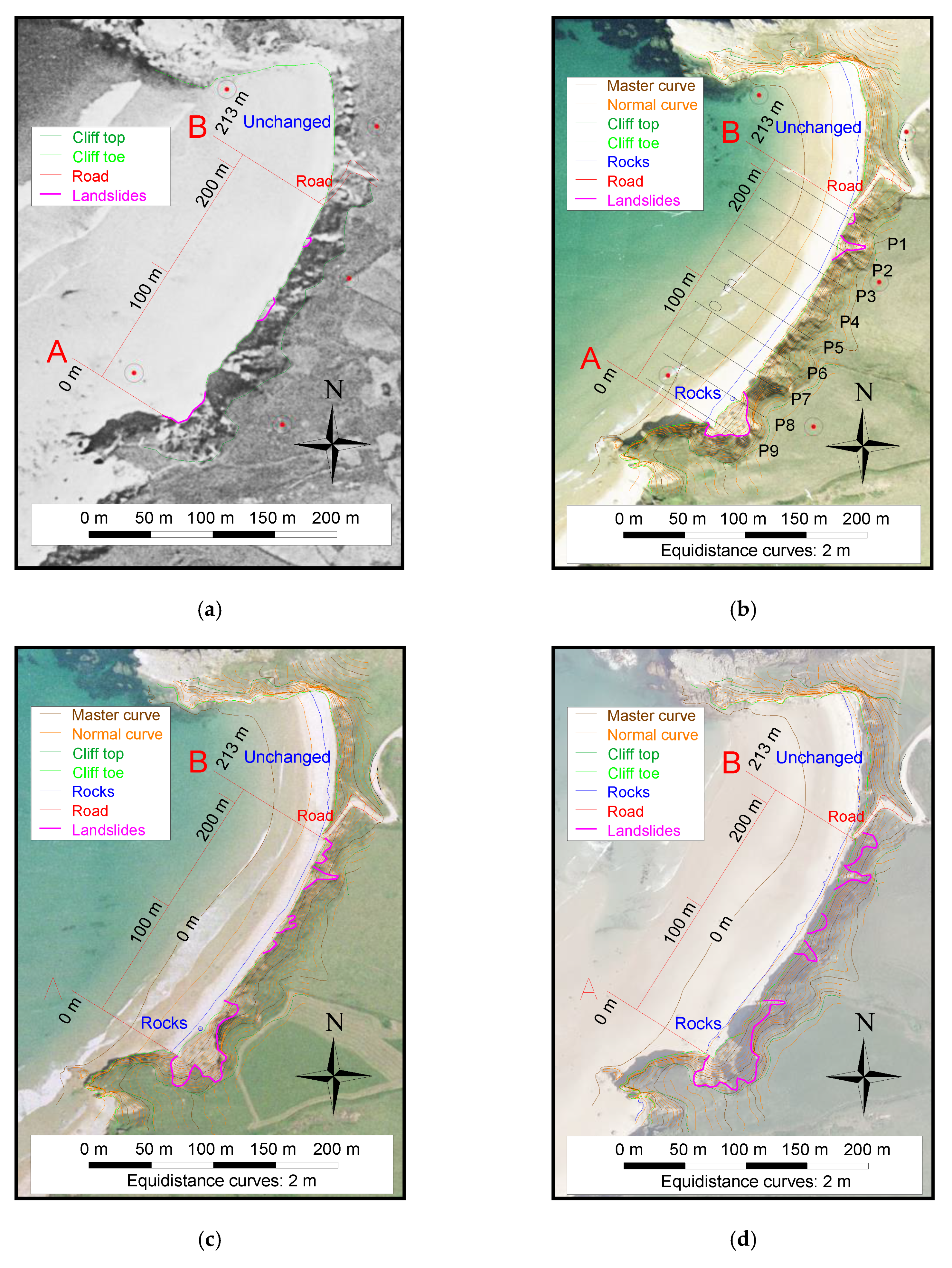
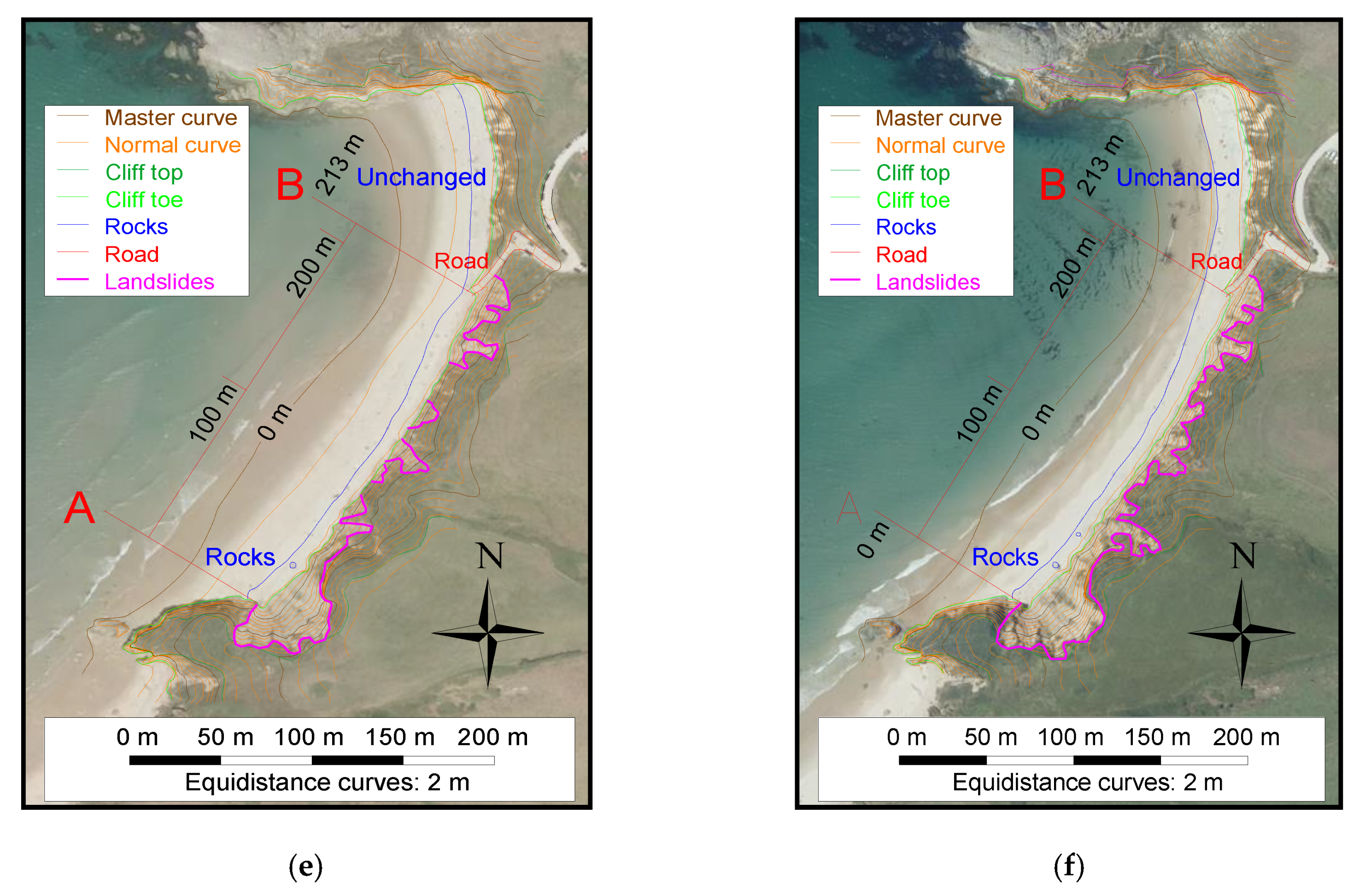
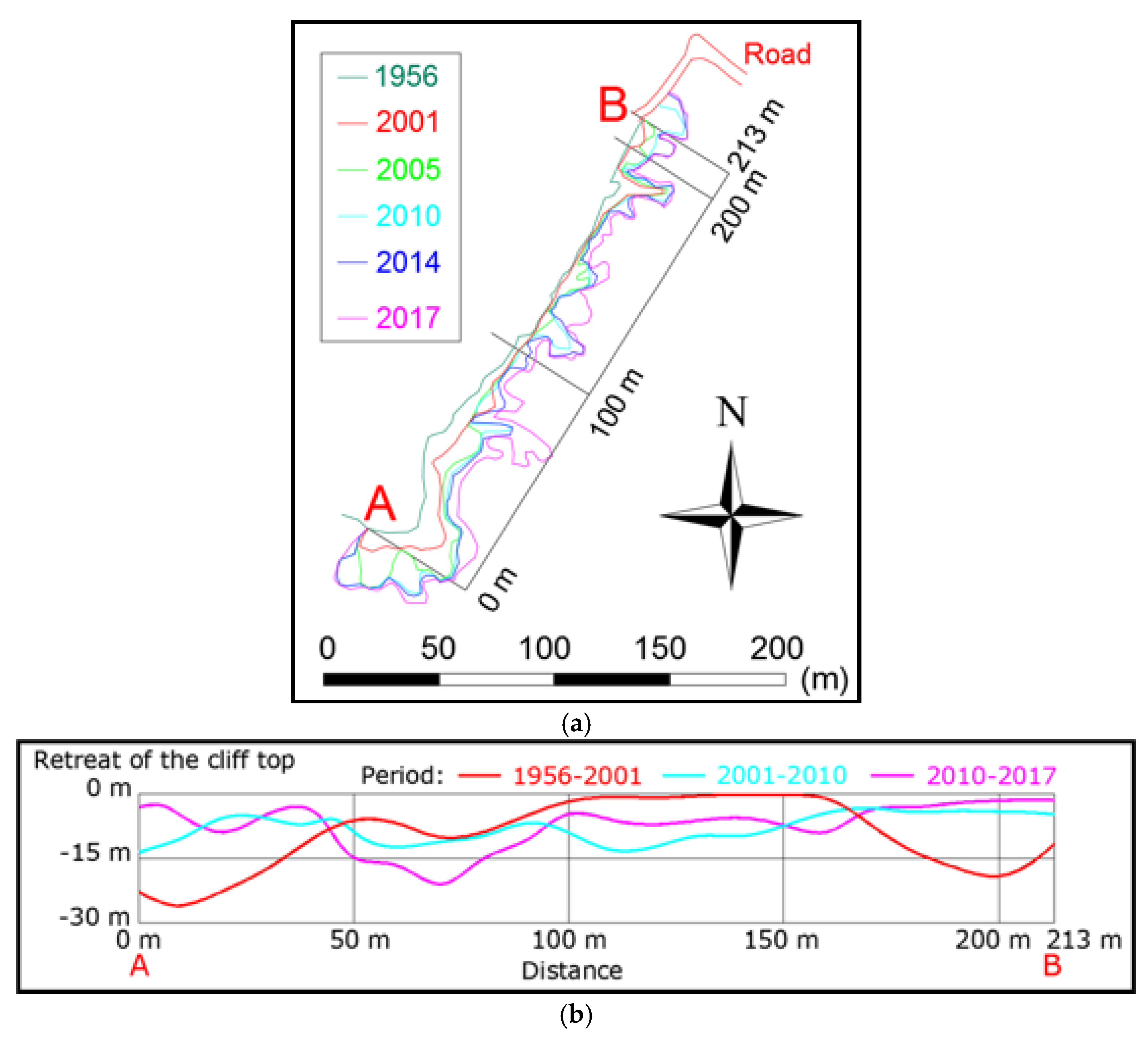
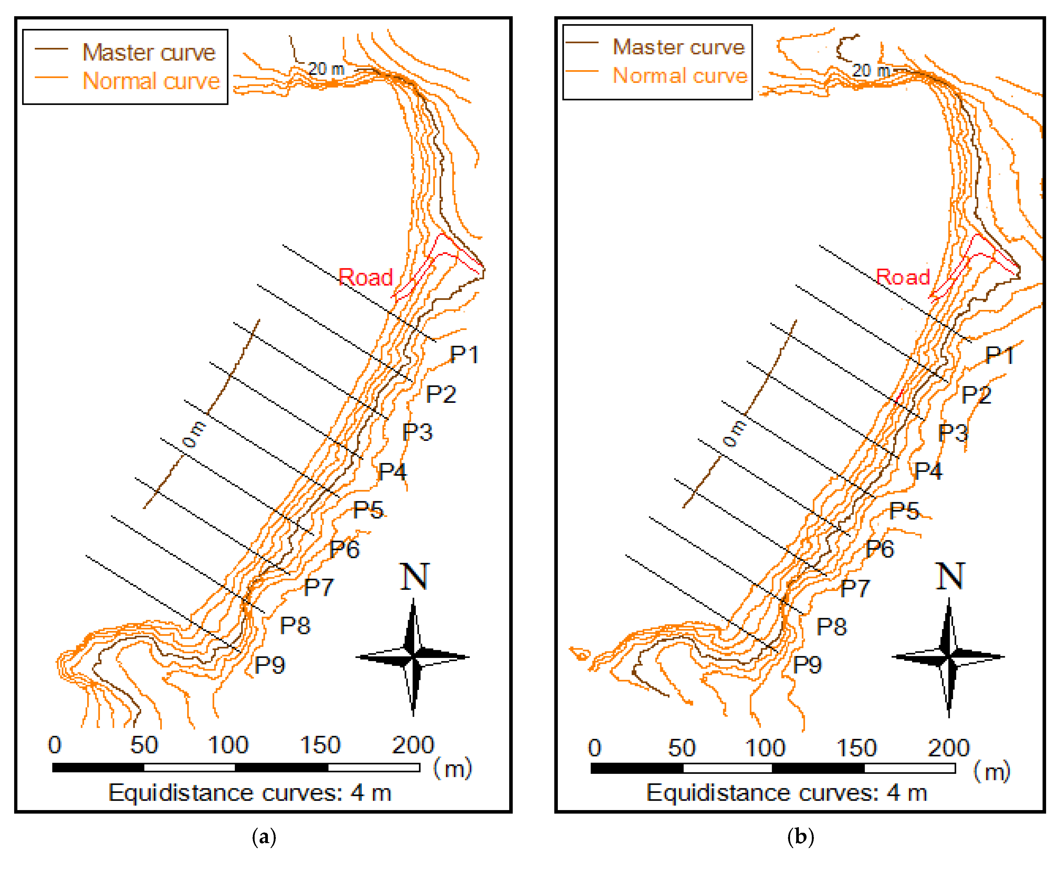
4.1. Applying Aerial Photogrammetry (1956–2017)
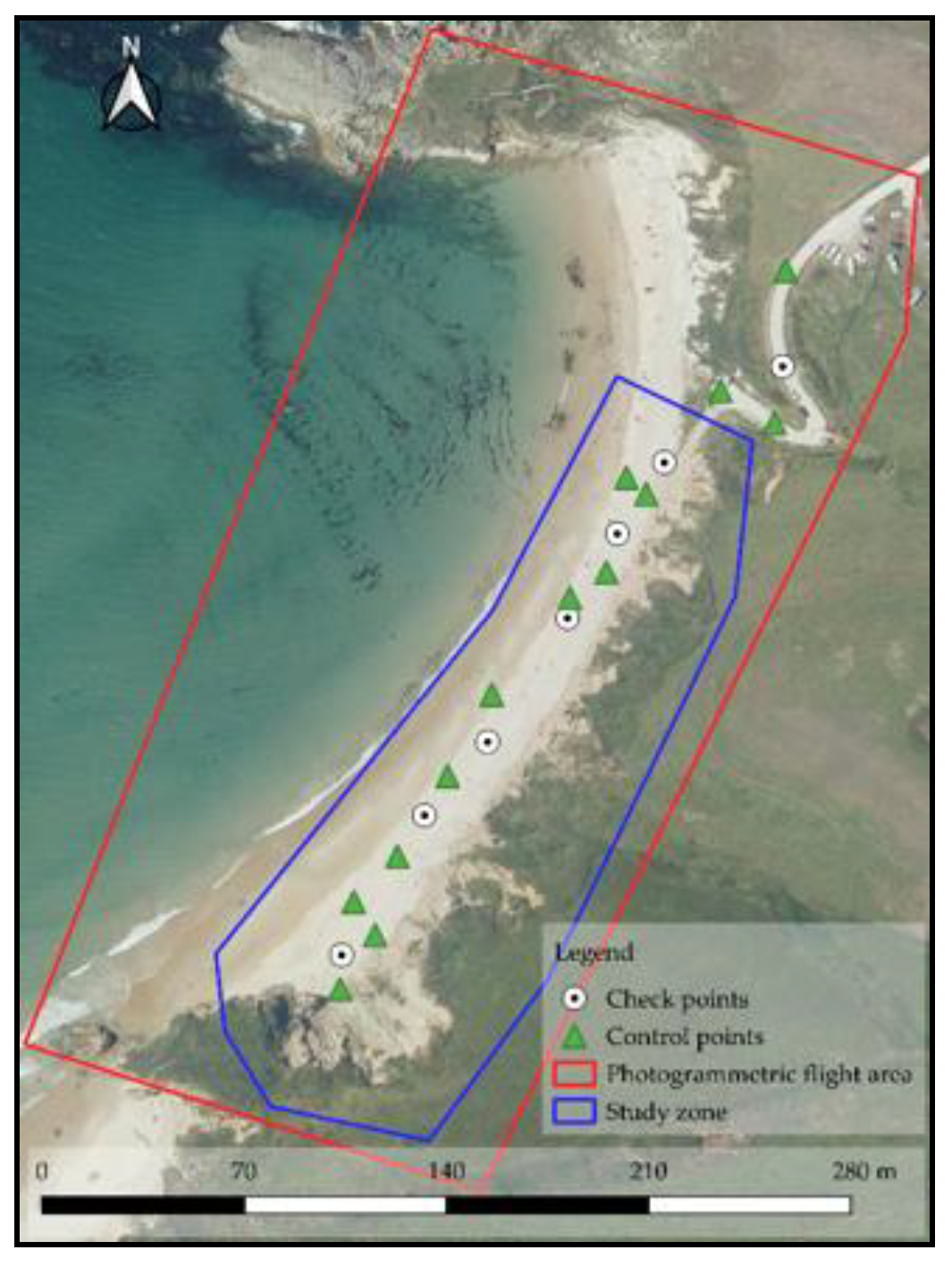
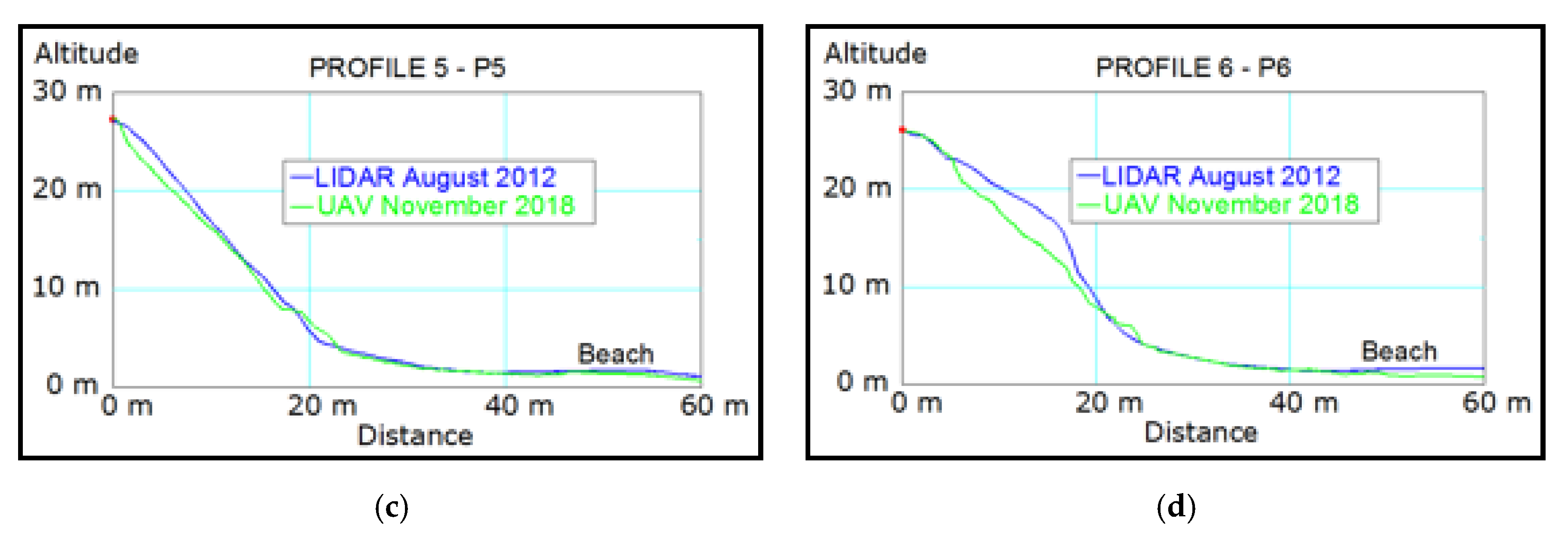
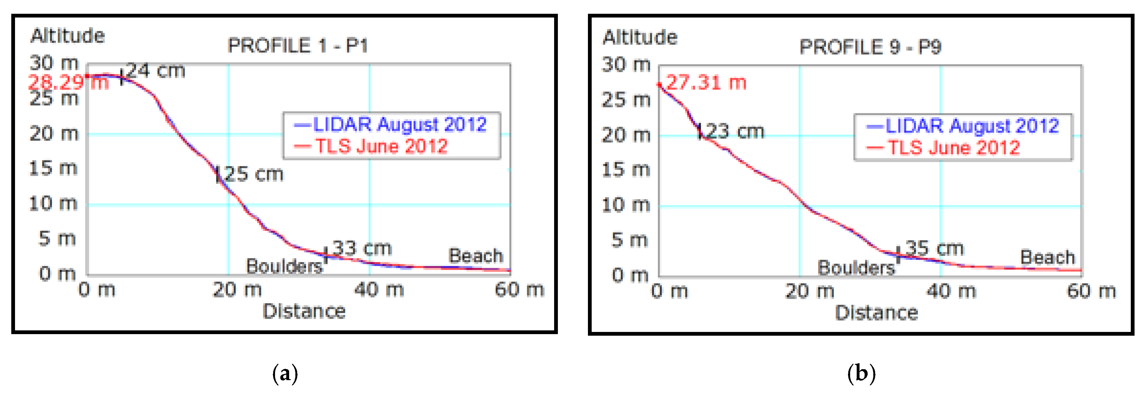
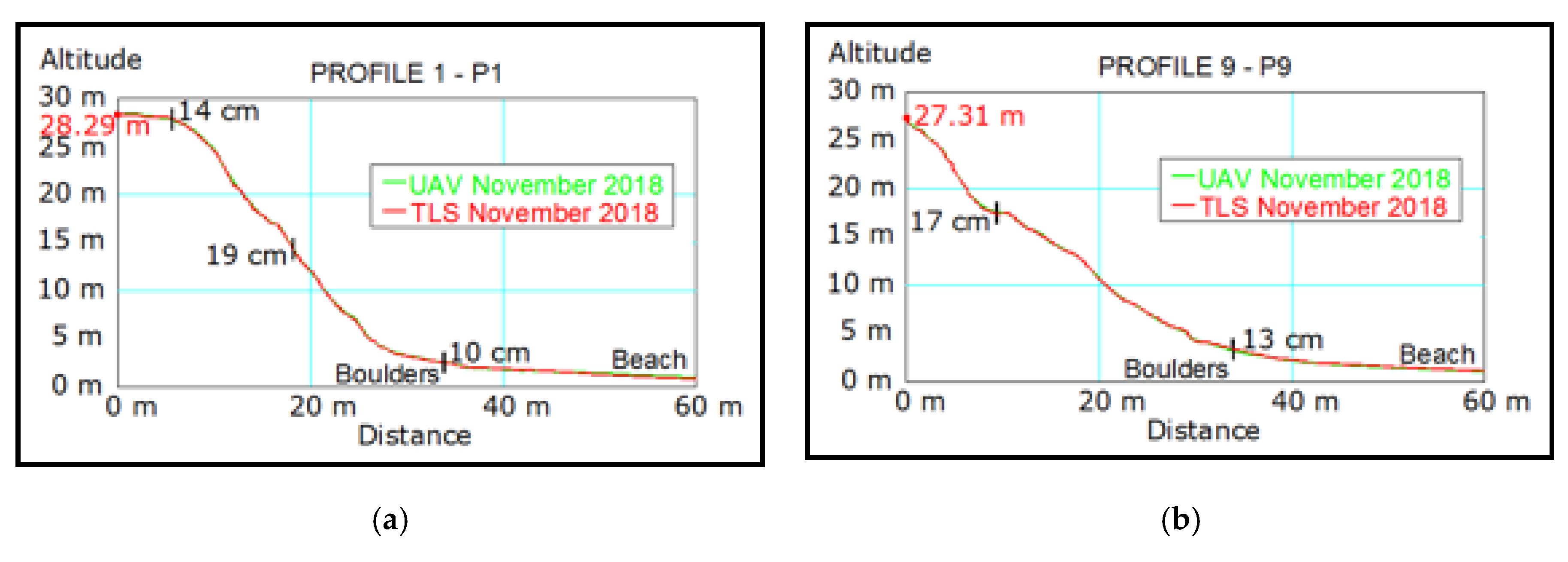
4.2. Applying Light Detection and Ranging (LiDAR) (August 2012) and Unmanned Aerial Vehicle (UAV) (November 2018)
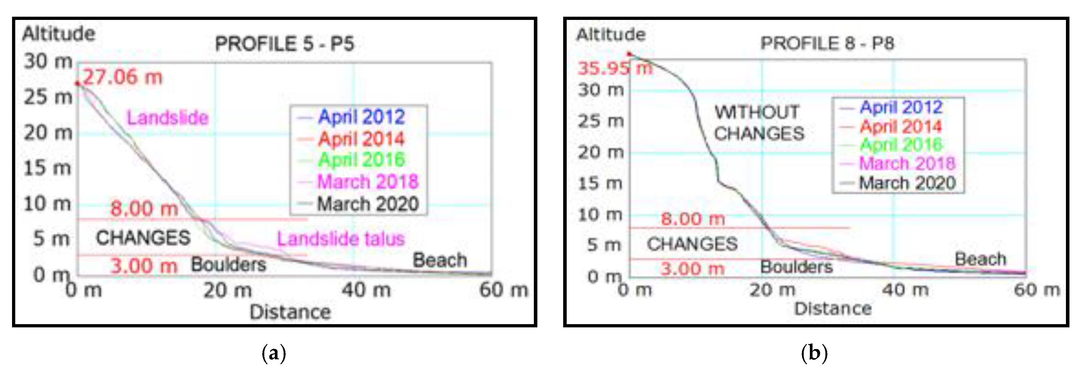
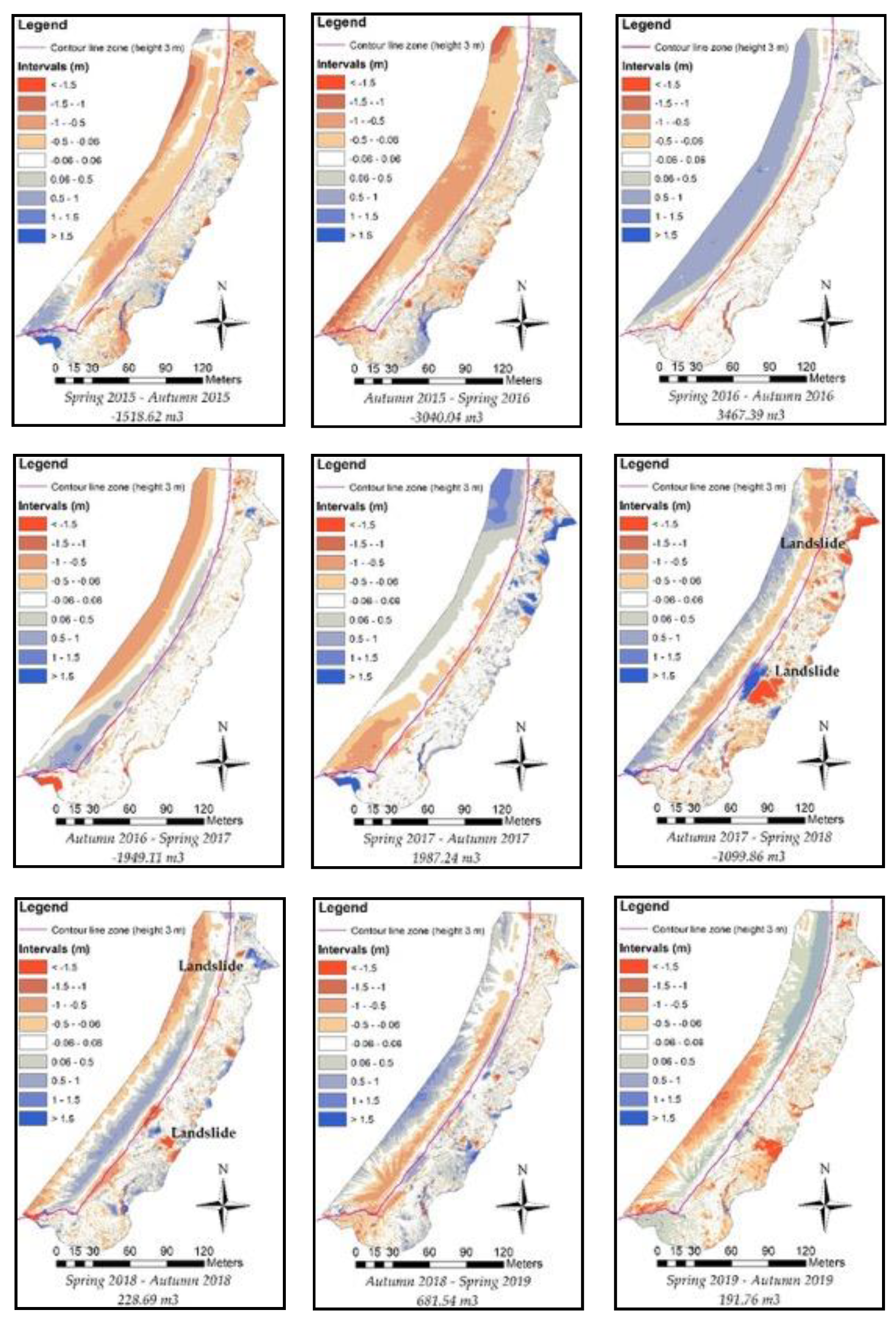
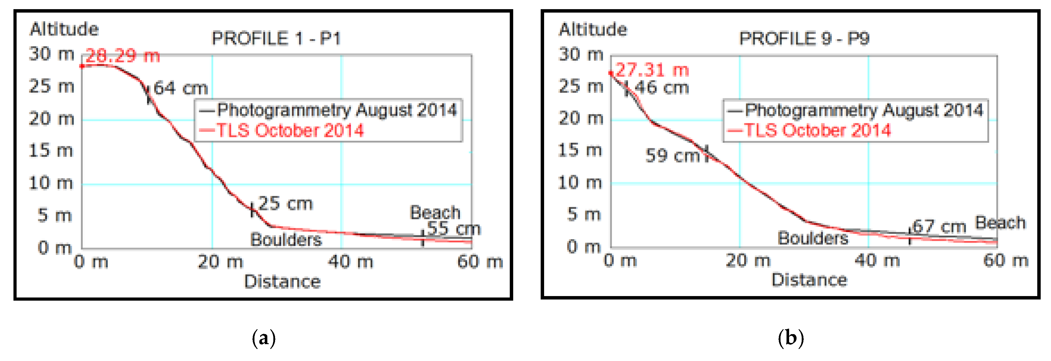
4.3. Applying Terrestrial Laser Scanning (2012–2020)
- In general, the semiannual altimetric variations were within the interval of 0 to ±0.5 m. In rare situations there were differences between ±0.5 and ±1 m, and differences higher than ±1 m are very rare.
- Small and large landslides were detected in DEMs. Large landslides, in some cases were caused by storms, for example, between the fall of 2013 and the spring of 2014; in other cases, the landslides were caused by the instability of the cliff.
- The total accumulated volume in the study area (beach and cliff), from the spring of 2012 to the present (April 2020), indicated a material gain of 399.66 m3. It was a very small, almost negligible, gain value for the eight-year period. But, depending on the campaigns, there could be greater differences (gains or losses) in the beach area. Thus, for example, on the one hand, between the spring of 2016 and the fall of 2016, there was a sand gain of 3467.39 m3, and on the other hand, between the fall of 2015 and the spring of 2016, there was a sand loss of −3040.04 m3.
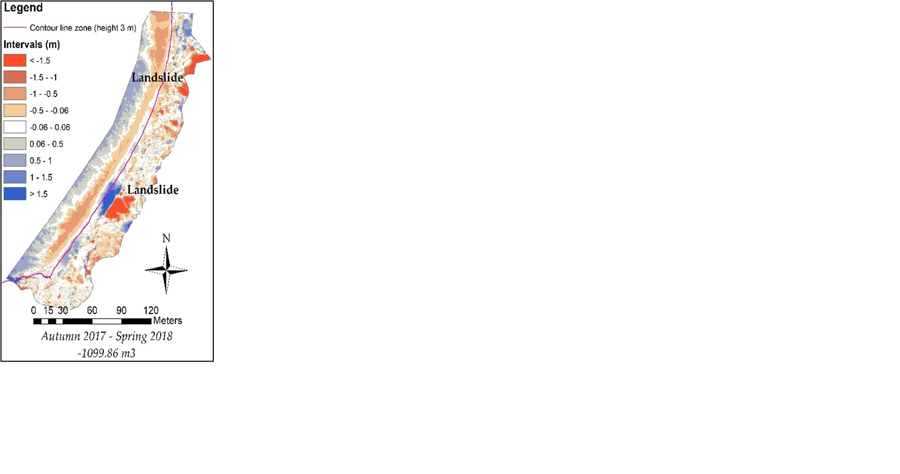
- The volumetric values that occurred above the base line of the cliff (3 meters above sea level) were also analyzed. At 3 meters altitude, small landslides occurred (for example, between the fall of 2013 and the spring of 2014). There were also large landslides across the cliff (for example, between the fall of 2017 and the spring of 2018). Throughout the study period, the total loss of material that occurred in the cliff area was −3633.32 m3.
5. Discussion
- The TLS can generate occlusions when the laser pulses hit a surface at an oblique angle from the scanner point of view (beach). The image processing algorithms used with the UAV photographs can generate occlusions on surfaces that have little inherent contrast or texture of color (beach area). This results in a dependency of the precision of each method on the landscape in question [71].
- The TLS and UAV methods are capable of collecting data at very different spatial scales. This has a substantial influence on the application of these methods and needs to be considered when making a comparison between them. In this case, the scale of both methods is very similar, since the measurement errors are ± 4 cm.
6. Conclusions
Author Contributions
Funding
Conflicts of Interest
References
- Mushkin, A.; Katz, O.; Porat, N. Overestimation of short-term coastal cliff retreat rates in the eastern Mediterranean resolved with a sediment budget approach. Earth Surf. Process. Landf. 2019, 44, 179–190. [Google Scholar] [CrossRef] [Green Version]
- Sunamura, T. Rocky coast processes: With special reference to the recession of soft rock cliffs. Proc. Japan Acad. Ser. B Phys. Biol. Sci. 2015, 91, 481–500. [Google Scholar] [CrossRef] [PubMed] [Green Version]
- Costa, S.; Maquaire, O.; Letortu, P.; Thirard, G.; Compain, V.; Roulland, T.; Medjkane, M.; Davidson, R.; Graff, K.; Lissak, C. Sedimentary Coastal cliffs of Normandy: Modalities and quantification of retreat. J. Coast. Res. 2019, 88, 46–60. [Google Scholar] [CrossRef]
- Young, A.P.; Carilli, J.E. Global distribution of coastal cliffs. Earth Surf. Process. Landf. 2019, 44, 1309–1316. [Google Scholar] [CrossRef] [Green Version]
- Young, A.P. Decadal-scale coastal cliff retreat in southern and central California. Geomorphology 2018, 300, 164–175. [Google Scholar] [CrossRef]
- Losada, M.A.; Medina, R.; Vidal, C.; Roldan, A. Historical evolution and morphological analysis of “El Puntal” spit, Santander (Spain). J. Coast. Res. 1991, 7, 711–722. [Google Scholar]
- Garrote, J.; Garzón, G.; Page, J. Condicionamientos antrópicos en la erosión de la playa de Oyambre (Cantabria). In Proceedings of the Actas V Reunión de Cuaternario Ibérico, Lisbon, Coambra, Portugal, July 2001; Volume 1, pp. 67–70. [Google Scholar]
- Lorenzo, F.; Alonso, A.; Pagés, J.L. Erosion and accretion of beach and spit systems in Northwest Spain: A response to human activity. J. Coast. Res. 2007, 2007, 834–845. [Google Scholar] [CrossRef]
- Flor-Blanco, G.; Pando, L.; Morales, J.A.; Flor, G. Evolution of beach–dune fields systems following the construction of jetties in estuarine mouths (Cantabrian coast, NW Spain). Environ. Earth Sci. 2015, 73, 1317–1330. [Google Scholar] [CrossRef]
- Garrote, J.; Heydt, G.; Alcantara-Carrio, J. Influencia de Los temporales sobre el transporte de sedimentos en la Playa de Oyambre (Cantabria, N de España). In Proceedings of the Actas V Reunión Nacional de Geomorfología, Valladolid, Spain, 26 June 2002; pp. 361–371. [Google Scholar]
- Sanjosé, J.D.; Serrano, E.; Berenguer, F.; González-Trueba, J.J.; Gómez-Lende, M.; González-García, M.; Guerrero-Castro, M. Evolución histórica y actual de la línea de costa en la playa de Somo (Cantabria), mediante el empleo de la fotogrametría aérea y escáner láser terrestre. Cuaternario Geomorfol. 2016, 30, 119–130. [Google Scholar] [CrossRef] [Green Version]
- De Sanjosé Blasco, J.J.; Gómez-Lende, M.; Sánchez-Fernández, M.; Serrano-Cañadas, E. Monitoring retreat of coastal sandy systems using geomatics techniques: Somo Beach (Cantabrian Coast, Spain, 1875–2017). Remote Sens. 2018, 10, 25. [Google Scholar] [CrossRef] [Green Version]
- Arteaga, C.; Juan de Sanjose, J.; Serrano, E. Terrestrial photogrammetric techniques applied to the control of a parabolic dune in the Liencres dune system, Cantabria (Spain). Earth Surf. Process. Landf. 2008, 33, 2201–2210. [Google Scholar] [CrossRef]
- Letortu, P.; Costa, S.; Maquaire, O.; Delacourt, C.; Augereau, E.; Davidson, R.; Suanez, S.; Nabucet, J. Retreat rates, modalities and agents responsible for erosion along the coastal chalk cliffs of Upper Normandy: The contribution of terrestrial laser scanning. Geomorphology 2015, 245, 3–14. [Google Scholar] [CrossRef]
- Letortu, P.; Costa, S.; Bensaid, A.; Cador, J.-M.; Quénol, H. Vitesses et modalités de recul des falaises crayeuses de Haute-Normandie (France): Méthodologie et variabilité du recul. Géomorphologie Reli. Process. Environ. 2014, 20, 133–144. [Google Scholar] [CrossRef]
- Letortu, P.; Costa, S.; Cador, J.; Coinaud, C.; Cantat, O. Statistical and empirical analyses of the triggers of coastal chalk cliff failure. Earth Surf. Process. Landf. 2015, 40, 1371–1386. [Google Scholar] [CrossRef]
- Kuhn, D.; Prüfer, S. Coastal cliff monitoring and analysis of mass wasting processes with the application of terrestrial laser scanning: A case study of Rügen, Germany. Geomorphology 2014, 213, 153–165. [Google Scholar] [CrossRef]
- Young, A.P.; Ashford, S.A. Instability investigation of cantilevered seacliffs. Earth Surf. Process. Landf. J. Br. Geomorphol. Res. Group 2008, 33, 1661–1677. [Google Scholar] [CrossRef]
- Toimil, A.; Losada, I.J.; Camus, P.; Díaz-Simal, P. Managing coastal erosion under climate change at the regional scale. Coast. Eng. 2017, 128, 106–122. [Google Scholar] [CrossRef]
- Masselink, G.; Russell, P.; Rennie, A.; Brooks, S.; Spencer, T. Impacts of climate change on coastal geomorphology and coastal erosion relevant to the coastal and marine environment around the UK. MCCIP Sci. Rev. 2020, 2020, 158–189. [Google Scholar]
- Martínez, C.; Contreras-López, M.; Winckler, P.; Hidalgo, H.; Godoy, E.; Agredano, R. Coastal erosion in central Chile: A new hazard? Ocean Coast. Manag. 2018, 156, 141–155. [Google Scholar] [CrossRef]
- Bruno, M.; Molfetta, M.; Pratola, L.; Mossa, M.; Nutricato, R.; Morea, A.; Nitti, D.; Chiaradia, M. A Combined Approach of Field Data and Earth Observation for Coastal Risk Assessment. Sensors 2019, 19, 1399. [Google Scholar] [CrossRef] [Green Version]
- Valentini, N.; Saponieri, A.; Danisi, A.; Pratola, L.; Damiani, L. Exploiting remote imagery in an embayed sandy beach for the validation of a runup model framework. Estuar. Coast. Shelf Sci. 2019, 225, 106244. [Google Scholar] [CrossRef] [Green Version]
- Terefenko, P.; Paprotny, D.; Giza, A.; Morales-Nápoles, O.; Kubicki, A.; Walczakiewicz, S. Monitoring cliff erosion with LiDAR surveys and bayesian network-based data analysis. Remote Sens. 2019, 11, 843. [Google Scholar] [CrossRef] [Green Version]
- Young, A.P.; Guza, R.T.; O’Reilly, W.C.; Burvingt, O.; Flick, R.E. Observations of coastal cliff base waves, sand levels, and cliff top shaking. Earth Surf. Process. Landf. 2016, 41, 1564–1573. [Google Scholar] [CrossRef] [Green Version]
- Katz, O.; Mushkin, A. Characteristics of sea-cliff erosion induced by a strong winter storm in the eastern Mediterranean. Quat. Res. 2013, 80, 20–32. [Google Scholar] [CrossRef]
- Dornbusch, U.; Robinson, D.A.; Moses, C.A.; Williams, R.B.G. Temporal and spatial variations of chalk cliff retreat in East Sussex, 1873 to 2001. Mar. Geol. 2008, 249, 271–282. [Google Scholar] [CrossRef]
- Benumof, B.T.; Griggs, G.B. The dependence of seacliff erosion rates on cliff material properties and physical processes: San Diego County, California. Shore Beach 1999, 67, 29–41. [Google Scholar]
- Rosser, N.J.; Petley, D.N.; Lim, M.; Dunning, S.A.; Allison, R.J. Terrestrial laser scanning for monitoring the process of hard rock coastal cliff erosion. Q. J. Eng. Geol. Hydrogeol. 2005, 38, 363–375. [Google Scholar] [CrossRef]
- Young, A.P.; Ashford, S.A. Application of airborne LIDAR for seacliff volumetric change and beach-sediment budget contributions. J. Coast. Res. 2006, 22, 307–318. [Google Scholar] [CrossRef] [Green Version]
- Marques, F. Rates, patterns, timing and magnitude-frequency of cliff retreat phenomena. A case study on the west coast of Portugal. Zeitschrift für Geomorphol. New Folge Suppl. Vol. 2006, 144, 231–257. [Google Scholar]
- Pierre, G.; Lahousse, P. The role of groundwater in cliff instability: An example at Cape Blanc-Nez (Pas-de-Calais, France). Earth Surf. Process. Landf. J. Br. Geomorphol. Res. Group 2006, 31, 31–45. [Google Scholar] [CrossRef]
- Olsen, M.J.; Johnstone, E.; Driscoll, N.; Ashford, S.A.; Kuester, F. Terrestrial laser scanning of extended cliff sections in dynamic environments: Parameter analysis. J. Surv. Eng. 2009, 135, 161–169. [Google Scholar] [CrossRef]
- Hernández-Pacheco, F.; Amor, I.A. Fisiografía y sedimentología de la playa y ría de San Vicente de la Barquera (Santander). Estud. Geológicos 1966, 22, 1–23. [Google Scholar]
- Mary, G. Évolution de la Bordure Côtière Asturienne (Espagne) du Néogène á l´Actuel. Ph.D. Thesis, Université de Caen, Caen, France, 1979. [Google Scholar]
- Mary, G. Evolución del margen costero de la Cordillera Cantábrica en Asturias desde el Mioceno. Trab. Geol. 1983, 13, 3–37. [Google Scholar]
- González-Amuchástegui, M.J.; Serrano, E.; Edeso, J.M.; Meaza, G. Cambios del nivel del mar durante el Cuaternario y morfología litoral en la costa oriental cantábrica. (País Vasco y Cantabria). In Proceedings of the Geomorfologia Litoral i Quaternari; Sanjaume, E., Mateu, J., Eds.; Universitat de Valencia: Valencia, Spain, 2005; pp. 167–180. [Google Scholar]
- Flor, G.; Flor-Blanco, G. Raised beaches in the Cantabrian coast. In Landscapes and Landforms of Spain; Springer: Berlin/Heidelberg, Germany, 2014; pp. 239–248. [Google Scholar]
- Monino, M.; Diaz de Teran, J.R.; Cendrero, A. Variaciones del nivel del mar en la costa de Cantabria durante el Cuaternario. In Proceedings of the Reunión sobre el Cuaternario 7, Santander, Spain, 21–26 September 1987; pp. 233–236. [Google Scholar]
- Garzón, G.; Alonso, A.; Torres, T.; Llamas, J. Edad de las playas colgadas y de las turberas de Oyambre y Merón (Cantabria). Geogaceta 1996, 20, 498–501. [Google Scholar]
- IGME. Mapa Geológico de España E. 1/50.000. Comillas, No 33.; Ministerio de Industria (España): Madrid, Spain, 2009.
- IGME. Mapa Geológico de España E. 1/50.000. Comillas, No 33; Ministerio de Industria (España): Madrid, Spain, 1990.
- Gómez-Pazo, A.; Pérez-Alberti, A. Vulnerability of the Galician coast to marine storms in the context of global change. Sémata Cienc. Sociais Humanid. 2017, 29, 117–142. [Google Scholar]
- Pérez, J.A.; Bascon, F.M.; Charro, M.C. Photogrammetric usage of 1956-57 usaf aerial photography of Spain. Photogramm. Rec. 2014, 29, 108–124. [Google Scholar] [CrossRef]
- Soteres, C.; Rodríguez, A.F.; Martínez, J.; Ojeda, J.C.; Romero, E.; Abad, P.; Sánchez, A.; González, C.; Juanatey, M.; Ruiz, C.; et al. Publicación de datos LiDAR mediante servicios web estándar. In Proceedings of the II Jornadas Ibéricas de Infraestructuras de Datos Espaciales, Barcelona, Spain, 9–10 November 2011; Volume 2, p. 16. [Google Scholar]
- Sanjosé, J.J.; Martínez, E.; López, M.; Atkinson, A.D.J. Topografía Para Estudios de Grado; Universidad de Extremadura. Servicio de Publicaciones: Bellisco, Spain, 2013. [Google Scholar]
- Hoffmeister, D.; Tilly, N.; Curdt, C.; Aasen, H.; Ntageretzis, K.; Hadler, H.; Willershäuser, T.; Vött, A.; Bareth, G. Terrestrial laser scanning for coastal geomorphologic research in western Greece. Int. Arch. Photogramm. Remote Sens. Spat. Inf. Sci. 2012, 39, 511–516. [Google Scholar] [CrossRef] [Green Version]
- Lindenbergh, R.C.; Soudarissanane, S.S.; De Vries, S.; Gorte, B.G.H.; De Schipper, M.A. Aeolian beach sand transport monitored by terrestrial laser scanning. Photogramm. Rec. 2011, 26, 384–399. [Google Scholar] [CrossRef]
- González Amuchastegui, M.J.; Ibisate González de Matauco, A.; Rico Lozano, I.; Sánchez Fernández, M.; Sanjosé, J.J. Cambios geomorfológicos y evolución de una barra de arena en la desembocadura del río Lea, Lekeitio-Mendexa (Bizkaia). Cuaternario Geomorfol. 2016, 30, 75–85. [Google Scholar] [CrossRef] [Green Version]
- Bremer, M.; Sass, O. Combining airborne and terrestrial laser scanning for quantifying erosion and deposition by a debris flow event. Geomorphology 2012, 138, 49–60. [Google Scholar] [CrossRef]
- Jaboyedoff, M.; Oppikofer, T.; Abellán, A.; Derron, M.-H.; Loye, A.; Metzger, R.; Pedrazzini, A. Use of LIDAR in landslide investigations: A review. Nat. Hazards 2012, 61, 5–28. [Google Scholar] [CrossRef] [Green Version]
- Hansom, J.D. Coastal sensitivity to environmental change: A view from the beach. Catena 2001, 42, 291–305. [Google Scholar] [CrossRef]
- Hall, A.M.; Hansom, J.D.; Jarvis, J. Patterns and rates of erosion produced by high energy wave processes on hard rock headlands: The Grind of the Navir, Shetland, Scotland. Mar. Geol. 2008, 248, 28–46. [Google Scholar] [CrossRef] [Green Version]
- Flor, G.; Flor-Blanco, G.; Flores-Soriano, C.; Alcántara-Carrió, J.; Montoya-Mpontes, I. Efectos de los temporales de invierno de 2014 sobre la costa asturiana. VIII Jorn. Geomorfol. Litoral Geo-Temas 2015, 15, 17–20. [Google Scholar]
- Catalão, J.; Catita, C.; Miranda, J.; Dias, J. Photogrammetric analysis of the coastal erosion in the Algarve (Portugal). Géomorphologie Reli. Process. Environ. 2002, 8, 119–126. [Google Scholar] [CrossRef] [Green Version]
- Esposito, G.; Salvini, R.; Matano, F.; Sacchi, M.; Troise, C. Evaluation of geomorphic changes and retreat rates of a coastal pyroclastic cliff in the Campi Flegrei volcanic district, southern Italy. J. Coast. Conserv. 2018, 22, 957–972. [Google Scholar] [CrossRef]
- Marques, F. Regional scale sea cliff hazard assessment at sintra and cascais counties, western coast of Portugal. Geoscience 2018, 8, 80. [Google Scholar] [CrossRef] [Green Version]
- Gómez-Pazo, A.; Pérez-Alberti, A.; Pérez, X.L.O. Recent evolution (1956–2017) of rodas beach on the Cíes Islands, Galicia, NW Spain. J. Mar. Sci. Eng. 2019, 7, 125. [Google Scholar] [CrossRef] [Green Version]
- Earlie, C.S.; Masselink, G.; Russell, P.E.; Shail, R.K. Application of airborne LiDAR to investigate rates of recession in rocky coast environments. J. Coast. Conserv. 2015, 19, 831–845. [Google Scholar] [CrossRef]
- Gonçalves, J.A.; Henriques, R. UAV photogrammetry for topographic monitoring of coastal areas. ISPRS J. Photogramm. Remote Sens. 2015, 104, 101–111. [Google Scholar] [CrossRef]
- Long, N.; Millescamps, B.; Guillot, B.; Pouget, F.; Bertin, X. Monitoring the topography of a dynamic tidal inlet using UAV imagery. Remote Sens. 2016, 8, 387. [Google Scholar] [CrossRef] [Green Version]
- Mancini, F.; Castagnetti, C.; Rossi, P.; Dubbini, M.; Fazio, N.L.; Perrotti, M.; Lollino, P. An integrated procedure to assess the stability of coastal rocky cliffs: From UAV close-range photogrammetry to geomechanical finite element modeling. Remote Sens. 2017, 9, 1235. [Google Scholar] [CrossRef] [Green Version]
- Westoby, M.J.; Lim, M.; Hogg, M.; Pound, M.J.; Dunlop, L.; Woodward, J. Cost-effective erosion monitoring of coastal cliffs. Coast. Eng. 2018, 138, 152–164. [Google Scholar] [CrossRef]
- Gómez-Gutiérrez, Á.; De Sanjosé-Blasco, J.J.; Lozano-Parra, J.; Berenguer-Sempere, F.; De Matías-Bejarano, J. Does HDR pre-processing improve the accuracy of 3D models obtained by means of two conventional SfM-MVS software packages? The case of the corral del veleta rock glacier. Remote Sens. 2015, 7, 10269–10294. [Google Scholar] [CrossRef] [Green Version]
- Crawford, A.J.; Mueller, D.; Joyal, G. Surveying drifting icebergs and ice islands: Deterioration detection and mass estimation with aerial photogrammetry and laser scanning. Remote Sens. 2018, 10, 575. [Google Scholar] [CrossRef] [Green Version]
- Jaud, M.; Kervot, M.; Delacourt, C.; Bertin, S. Potential of smartphone SfM photogrammetry to measure coastal morphodynamics. Remote Sens. 2019, 11, 2242. [Google Scholar] [CrossRef] [Green Version]
- Hayakawa, Y.S.; Obanawa, H. Volumetric change detection in bedrock coastal cliffs using terrestrial laser scanning and uas-based SFM. Sensors 2020, 20, 3403. [Google Scholar] [CrossRef]
- Lichti, D.D.; Gordon, S.; Stewart, M.; Franke, J.; Tsakiri, M. Comparison of digital photogrammetry and laser scanning. In Proceedings of the CIPA W6 International Workshop, Corfu, Greece, 1–2 September 2002; pp. 39–47. [Google Scholar]
- Martin, C.D.; Tannant, D.D.; Lan, H. Comparison of terrestrial-based, high resolution, LiDAR and digital photogrammetry surveys of a rock slope. In Proceedings of the Proceedings 1st Canada-US Rock Mechanics Symp, British, DC, Canada, 27–31 May 2007; pp. 37–44. [Google Scholar]
- Sturzenegger, M.; Stead, D. Close-range terrestrial digital photogrammetry and terrestrial laser scanning for discontinuity characterization on rock cuts. Eng. Geol. 2009, 106, 163–182. [Google Scholar] [CrossRef]
- Seymour, A.C.; Ridge, J.T.; Rodriguez, A.B.; Newton, E.; Dale, J.; Johnston, D.W. Deploying Fixed Wing Unoccupied Aerial Systems (UAS) for Coastal Morphology Assessment and Management. J. Coast. Res. 2018, 34, 704–717. [Google Scholar] [CrossRef]


| Point | Coordenate | Year 2001 (m) | Year 2005 (m) | Year 2010 (m) | Year 2014 (m) | Year 2017 (m) | Difference in X (m) | Difference in Y (m) | Difference in Z (m) |
|---|---|---|---|---|---|---|---|---|---|
| X | 390,237.57 | 390,237.21 | 390,237.02 | 390,237.10 | 390,237.06 | 0.55 m | |||
| 1 | Y | 4,806,117.60 | 4,806,117.49 | 4,806,117.90 | 4,806,117.18 | 4,806,117.65 | 0.72 m | ||
| Z | 4.91 | 4.73 | 4.39 | 5.00 | 4.97 | 0.61 m | |||
| X | 390,044.87 | 390,044.19 | 390,044.75 | 390,045.10 | 390,044.55 | 0.91 m | |||
| 2 | Y | 4,805,844.06 | 4,805,845.03 | 4,805,844.98 | 4,805,844.07 | 4,805,844.72 | 0.97 m | ||
| Z | 45.31 | 45.27 | 45.90 | 45.53 | 45.45 | 0.63 m | |||
| X | 389,796.87 | 389,796.10 | 389,796.40 | 389,797.09 | 389,796.61 | 0.99 m | |||
| 3 | Y | 4,805,508.43 | 4,805,509.06 | 4,805,508.93 | 4,805,508.11 | 4,805,508.49 | 0.95 m | ||
| Z | 38.25 | 37.98 | 38.60 | 38.28 | 37.99 | 0.62 m | |||
| X | 389,765.01 | 389,764.28 | 389,764.67 | 389,765.18 | 389,764.65 | 0.90 m | |||
| 4 | Y | 4,805,185.22 | 4,805,186.14 | 4,805,186.12 | 4,805,185.18 | 4,805,185.60 | 0.96 m | ||
| Z | 53.78 | 53.19 | 53.29 | 53.75 | 53.42 | 0.59 m |
| Date (Year) | Information | Maximum Error (m) | Result |
|---|---|---|---|
| 1956 | Ortophotography | 2 m | Digitization |
| 200–2005–2010–2014–2017 | Aerial photogrammetry | 1 m | Cartography by restitution photogrammetric |
| August 2012 | LiDAR | 0.20 m | DEM |
| November 2018 | UAV | 0.04 m | DEM |
| 2012–2020 (Semiannual measurements, spring and fall) | TLS | 0.03 m | DEM |
Publisher’s Note: MDPI stays neutral with regard to jurisdictional claims in published maps and institutional affiliations. |
© 2020 by the authors. Licensee MDPI, Basel, Switzerland. This article is an open access article distributed under the terms and conditions of the Creative Commons Attribution (CC BY) license (http://creativecommons.org/licenses/by/4.0/).
Share and Cite
de Sanjosé Blasco, J.J.; Serrano-Cañadas, E.; Sánchez-Fernández, M.; Gómez-Lende, M.; Redweik, P. Application of Multiple Geomatic Techniques for Coastline Retreat Analysis: The Case of Gerra Beach (Cantabrian Coast, Spain). Remote Sens. 2020, 12, 3669. https://0-doi-org.brum.beds.ac.uk/10.3390/rs12213669
de Sanjosé Blasco JJ, Serrano-Cañadas E, Sánchez-Fernández M, Gómez-Lende M, Redweik P. Application of Multiple Geomatic Techniques for Coastline Retreat Analysis: The Case of Gerra Beach (Cantabrian Coast, Spain). Remote Sensing. 2020; 12(21):3669. https://0-doi-org.brum.beds.ac.uk/10.3390/rs12213669
Chicago/Turabian Stylede Sanjosé Blasco, José Juan, Enrique Serrano-Cañadas, Manuel Sánchez-Fernández, Manuel Gómez-Lende, and Paula Redweik. 2020. "Application of Multiple Geomatic Techniques for Coastline Retreat Analysis: The Case of Gerra Beach (Cantabrian Coast, Spain)" Remote Sensing 12, no. 21: 3669. https://0-doi-org.brum.beds.ac.uk/10.3390/rs12213669