Article

Estimating Fuel Loads and Structural Characteristics of Shrub Communities by Using Terrestrial Laser Scanning

by
Cecilia Alonso-Rego
1,
Stéfano Arellano-Pérez
1,
Carlos Cabo
2,3,
Celestino Ordoñez
2,
Juan Gabriel Álvarez-González
1,
Ramón Alberto Díaz-Varela
4 and
Ana Daría Ruiz-González
1,*
1
Departamento de Ingeniería Agroforestal, Escola Politécnica Superior de Enxeñaría, Universidade de Santiago de Compostela, Campus Universitario s/n, 27002 Lugo, Spain
2
Departamento de Explotación y Prospección de Minas, Universidad de Oviedo, 33003 Oviedo, Spain
3
College of Science, Swansea University, Singleton Campus, Swansea SA2 8PP, UK
4
GI-1809-BioAplic, Departamento de Botánica, Escola Politécnica Superior de Enxeñaría, Universidade de Santiago de Compostela, Campus Universitario s/n, 27002 Lugo, Spain
*
Author to whom correspondence should be addressed.
Remote Sens. 2020, 12(22), 3704; https://0-doi-org.brum.beds.ac.uk/10.3390/rs12223704
Submission received: 16 October 2020 / Revised: 4 November 2020 / Accepted: 9 November 2020 / Published: 11 November 2020
(This article belongs to the Special Issue 3D Point Clouds in Forest Remote Sensing)

Abstract

:
Forest fuel loads and structural characteristics strongly affect fire behavior, regulating the rate of spread, fireline intensity, and flame length. Accurate fuel characterization, including disaggregation of the fuel load by size classes, is therefore essential to obtain reliable predictions from fire behavior simulators and to support decision-making in fuel management and fire hazard prediction. A total of 55 sample plots of four of the main non-tree covered shrub communities in NW Spain were non-destructively sampled to estimate litter depth and shrub cover and height for species. Fuel loads were estimated from species-specific equations. Moreover, a single terrestrial laser scanning (TLS) scan was collected in each sample plot and features related to the vertical and horizontal distribution of the cloud points were calculated. Two alternative approaches for estimating size-disaggregated fuel loads and live/dead fractions from TLS data were compared: (i) a two-steps indirect estimation approach (IE) based on fitting three equations to estimate shrub height and cover and litter depth from TLS data and then use those estimates as inputs of the existing species-specific fuel load equations by size fractions based on these three variables; and (ii) a direct estimation approach (DE), consisting of fitting seven equations, one for each fuel fraction, to relate the fuel load estimates to TLS data. Overall, the direct approach produced more balanced goodness-of-fit statistics for the seven fractions considered jointly, suggesting that it performed better than the indirect approach, with equations explaining more than 80% of the observed variability for all species and fractions, except the litter loads.

1. Introduction

Fuel load, defined as the fuel dry biomass per unit area, is a particularly important forest fuel characteristic [1,2] as it represents the amount of live and dead biomass available for ignition and combustion. Along with other structural characteristics, fuel load strongly affects fire behavior, regulating the rate of spread, fireline intensity, and flame length [3,4]. Accurate fuel characterization, including the fuel load disaggregated by size classes and vegetative status (live and dead fractions), is essential to obtain reliable predictions from fire behavior simulators in order to support decision-making in fuel management and fire hazard prediction [5,6]. Fuel load is also an essential component in carbon cycle assessment and in models used to predict fire emissions and smoke impacts [7,8,9,10].
In the NW Iberian Peninsula, the fast shrub growth associated with mild annual temperatures and high rainfall promotes large accumulations of surface fuel that favor high intensity surface wildfires [11]. Indeed, the area is one of the most severely affected by fire in Europe [12,13]. Recent studies have reported an increase in fire activity in terms of both frequency and burnt area, mainly corresponding to eastern flows during summer, with a substantial contribution from southeastern advections in winter [14,15,16]. In Galicia, located in the westernmost part of this region, the problem is especially important in shrublands, as 63% of the total area burned in this region in the last 20 years has affected non-tree shrub communities [17], even though these communities represent only about 30% of the total forest area and 20% of the total area of the region [18].
The fuel load of shrub communities, i.e., shrub and litter layers, can be quantified by different methods, including destructive and non-destructive sampling [19]. Destructive sampling is the most accurate method of determining fuel load, but also the most complex and costly in time and money, and it is therefore difficult to apply to large areas [2,20]. Non-destructive sampling enables indirect estimation of the fuel load, usually by using allometric relationships between fuel loads and fuel characteristics that are easily measured in the field [21,22,23].
In the last two decades new models relating fuelbed characteristics to remotely sensed data have been developed by using information obtained from satellite images [24,25,26,27,28] or airborne laser scanner (ALS) data [29,30,31,32,33]. This has enabled the construction of thematic fuel maps for fire simulation and fire risk assessment. However, the accuracy of the model estimates largely depends on the accuracy of the digital terrain model (DTM) generated, which is, in turn, affected by the density of the vegetation and the orography [34]. Thus, in very dense shrubland and rugged terrain, typical of the Galician territory, shrub height and volume tend to be underestimated [35,36,37].
Terrestrial laser scanning (TLS) has evolved as a non-destructive measurement technique that produces data (3D point clouds) of great potential for use in forestry applications. Such uses include the assessment of tree and stand level biomass and carbon [38,39,40,41] and also the accurate quantification of relevant fuelbed characteristics for determining fire behavior, fuel consumed and smoke emissions [42,43,44,45]. In addition, studies in which TLS data are combined or compared with ALS data [46,47,48,49,50], data from unmanned aerial vehicles [51,52] or satellite images [53] have become more frequent in recent years for various forestry applications.
Most TLS-based studies estimating shrub biomass or volume have focused on the reconstruction of the shrub shape from the point cloud, either by piecewise approximation of the volume or by voxelization. For example, Olsoy et al. [43] estimated the biomass of sagebrush (Artemisia tridentata) using both voxel counting and a 3-D convex hull approach, concluding that the 3-D convex hull model estimated total and green biomass more accurately than the voxelization approach. Greaves et al. [54] also compared both approaches for estimating harvested biomass of two dominant Alaskan tundra shrub species, using point clouds obtained from close-range (2 m) and variable-range (<50 m) TLS, and reported better results for voxel counting in close-range data and stronger relationships for the surface difference approach for variable-range data. Hudak et al. [49] and Rowell et al. [55] adapted the “3D field sampling protocol” proposed by Hawley et al. [56] to infer fine-scale fuel mass in 3D, observing that mass was strongly related to the voxel-occupancy volume, porosity, and surface area, which were used to develop equations for fine-scale prediction.
In general, fuel characterization studies with TLS are carried out in tree-covered shrub communities, often characterized by a heterogeneous spatial distribution on the ground, and they usually focus on obtaining detailed fuel information for applying physical-based fire models, such as WRF-SFIRE-CHEM [57,58], WFDSS [59,60], and FIRETEC [61,62], which require spatially explicit, three-dimensional data [63]. However, the use of TLS data should not be restricted to obtaining geometric information on a scale as detailed as that required for the use of physical-based models that operate in 3D, but should be tested for potential use in obtaining the fuel characteristics required for the application of more operational simulators such as Farsite and Flammap [64,65]. In addition, such detailed studies require several scans from different positions, often at least 5 to 9 scans, indicating a very time-consuming field inventory and subsequent processing of the point clouds to obtain a single cloud. Studies that use TLS to predict biomass distribution without reconstructing shapes from the returns are scarce. Accordingly, the aim of this study was to test the potential use of TLS data to provide accurate fuel load estimates of size-disaggregated shrub and litter and live/dead fractions for four of the main non-tree covered shrub communities in Galicia (NW Spain) by using data from a single scan. For this purpose, two alternative approaches will be compared, one direct estimation approach and a two-steps indirect estimation approach.

2. Materials and Methods

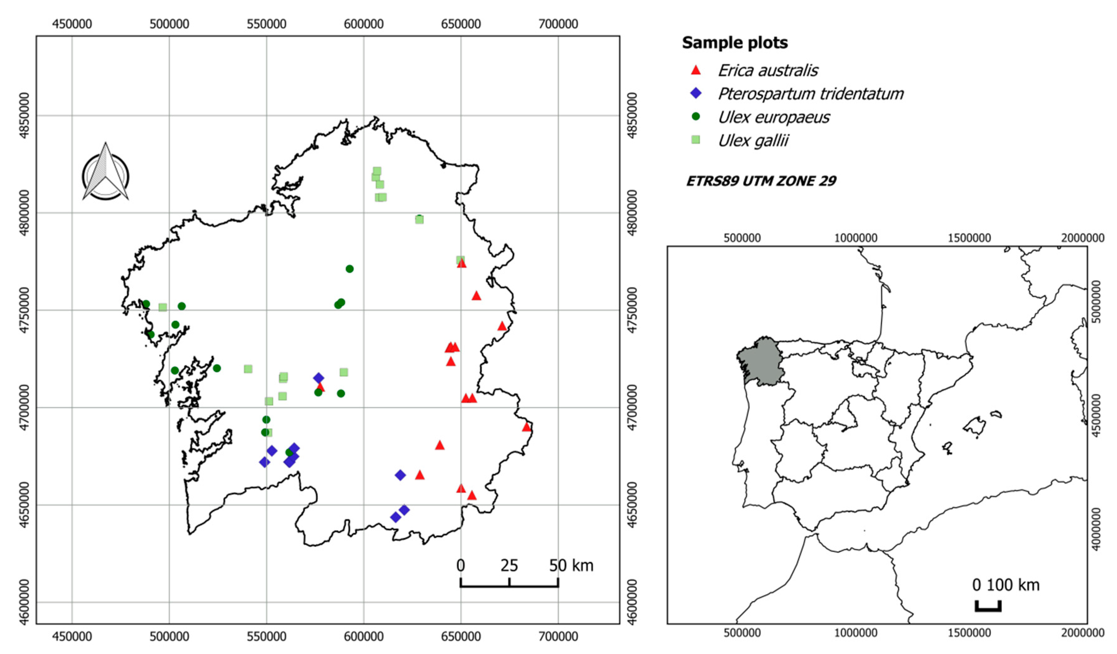
2.1. Shrub Communities and Plots

Shrubland areas in the study area (Galicia, NW Spain) are usually covered by gorse (genus Ulex), heath (genus Erica) and broom (genera Pterospartum, Cytisus and Genista), covering 55%, 22%, and 11% of the shrubland area, respectively [66]. Four treeless shrub communities were selected and characterized by the dominant species (Table 1). The communities selected are widely represented in Galicia [18,66] and are among the most frequently affected by wildfires in the region. All the communities considered are multiannual woody shrubs with stems branching from the base.
Subjective sampling was carried out to select a representative sample of each of the 4 shrub communities by taking the main structural fuel attributes observed in the study area into account. The plots were located using information obtained from different sources, particularly the Spanish Forest Map [66,67]. A total of 55 sample sites were selected in areas where the dominant shrub species of each community predominated, and shrub cover was higher than 80%. The spatial distribution of the sampled plots throughout the study area is shown in Figure 1.

2.2. Field Inventories and Determination of Fuel Characteristics
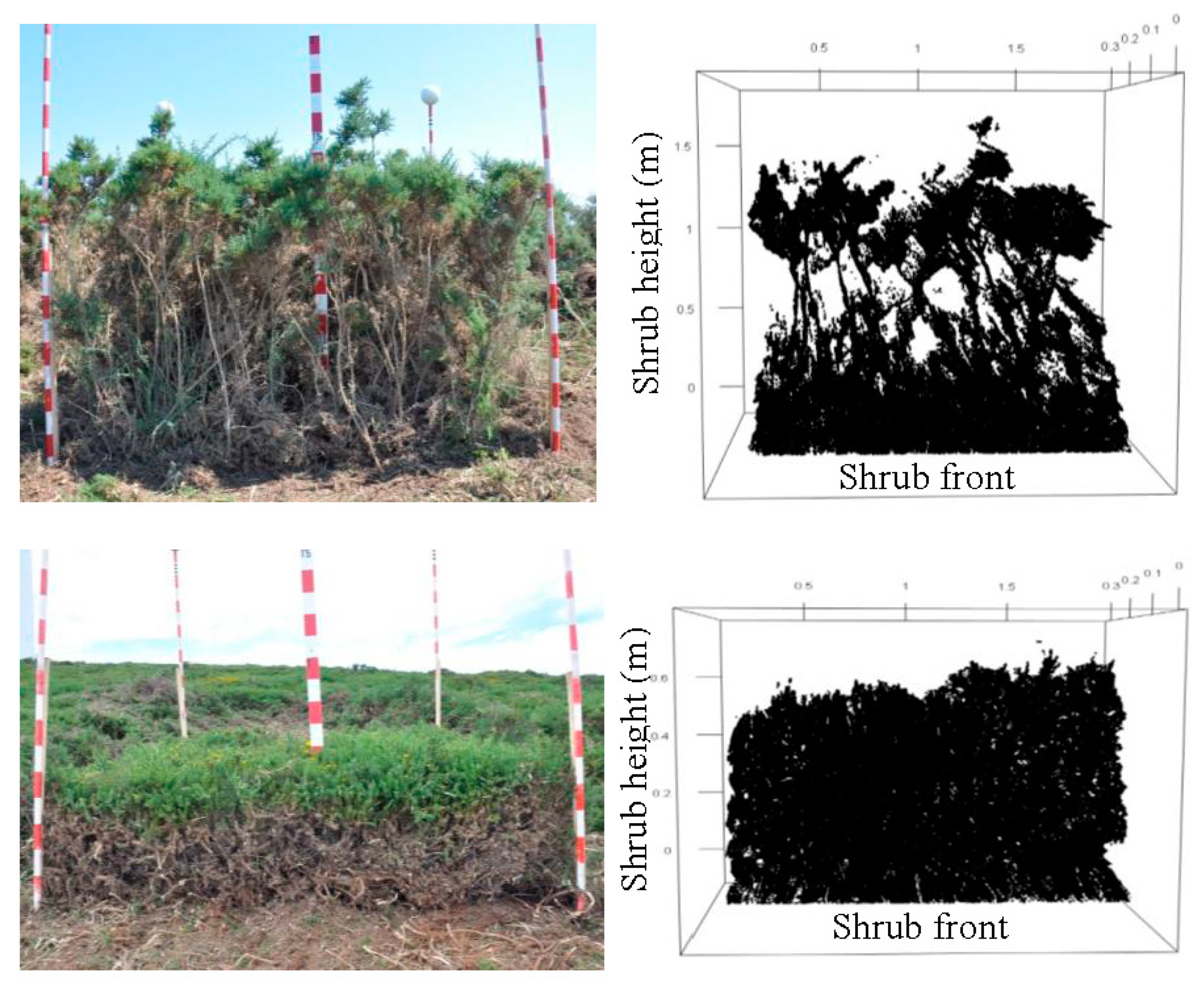
Field measurements were made in the shrub and litter layers of each sample plot by randomly locating a 2 × 2 m sampling square with sides parallel to the contour line and to the maximum slope. Each sampling square was delimited with four wooden stakes and all the vegetation in a 0.5-m strip around the square was removed, except the side where the TLS was located, where a 4-m strip of vegetation was removed.
A sampling transect consisting of the plot perimeter plus one diagonal of the square was outlined. The horizontal lengths of the intercepted shrub species (cm) were measured along this linear transect, to estimate the linear shrub cover (CovShr) according to the method proposed by Canfield [68]. Moreover, dead and live base height, total shrub height of the intercepted species (cm) and litter depth were also measured (every 50 cm). As the separation between the litter and duff layers is not always very clear in shrub communities, both layers were sampled together as litter. Shrub height was measured as the vertical distance between the litter layer and the top of vegetation. All the shrub and litter structural measurements were averaged to produce the mean shrub height ( h S h r ¯ ) and mean litter depth ( d L i t t ¯ ).
For each community, the fuel loads were estimated using the species-specific biomass equations systems at stand level developed for treeless shrub communities in Galicia [69], with CovShr, h S h r ¯ and d L i t t ¯ as inputs. These systems include equations for each of the following seven fractions: dead fine shrub load (diameter < 0.6 cm; WShr_G1_dead); live fine shrub load (diameter < 0.6 cm; WShr_G1_live); fine shrub load (diameter < 0.6 cm; WShr_G1, dead + live); coarse shrub load (diameter ≥ 0.6 cm; WShr_G23); total shrub load (WShr, fine + coarse); litter load (WLitt); and total shrub; and litter fuel load (WShr+Litt). The basic descriptive statistics of shrub and litter layers for the main structural characteristics of each shrub community are shown in Table 2.

2.3. TLS Data

Each sampling square was scanned once using a FARO Laser Scanner Focus3D X 130 TLS to collect three-dimensional point clouds with a density of ~7.67 mm point spacing at 10 m. The TLS is a class I laser (wavelength = 1550 nm) with a range of 0.6 to 130 m for objects with 90% reflectivity and with an accuracy of ±2 mm at 10 m range. Scanning was conducted by locating the TLS at a distance of 3 m from the contour line side of the square sampling located downhill.
The point clouds from the single scans on each sampling square were cropped and height was normalized. All points outside of the squares were removed, and the height above the terrain of each point (h) was calculated from digital elevation models (DEMs) created from each scan. DEMs were generated by interpolation, according to the lowest laser return within a 2 × 2 cm grid, in order to maintain consistency with the field measurements. The heights were then calculated by subtracting the smoothed DEM from the z values. These values were used to calculate 32 metrics related to the vertical distribution of the point clouds. The metrics and the corresponding descriptions are summarized in Table 3.
Due to shrub occlusions, the TLS-derived metrics vary as the depth of the analyzed laser returns cloud measured from the shrub front increases. Therefore, analysis was carried out to determine the optimum depth (measured from the vertical plane defined by the lowest side of the square) from which the metric values are stabilized, by comparing the values for depths varying from 10 to 50 cm, by 1 cm. This procedure is equivalent to constructing a virtual vertical plane parallel to the sampling square front and extracting all the points that are closer to the scanner than that plane. The results indicated that 30 cm depth of the laser returns cloud was adequate for all of the sampled plots, so the laser returns clouds were limited to this depth threshold (Figure 2).
The theoretical vertical shrub cover was estimated as the ratio between the observed number of laser returns and the maximum number of laser returns lrmax_ver. The maximum number was estimated considering the vertical plane defined by the lowest side of the square as a continuous solid with height equal to hmax and taking the laser scanner density into account. Moreover, the 3-D point clouds for each sample plot (2 × 2 × hmax) were divided into voxels (1 cm3), and the volume of shrub cover was calculated as the ratio between the number of voxels containing points and the total number of voxels. Both of these ratios were transformed by calculating the arcsine-square root of their values to stabilize the variance and improve normality [70], thus producing the Bliss variables TLSvCovShr and TLS3DCovShr. Finally, the vertical point distribution was modelled using the two-parameter Weibull probability density function (pdf). For this purpose, the relative frequency of the number of laser returns in each layer of height 1 cm and depth 30 cm was calculated by dividing the number of returns in this layer by the total number of laser returns. The scale (Wscale) and shape (Wshape) parameters of the Weibull pdf were then estimated using the first and the second moments of the relative distribution of vertical laser returns [71].
Point cloud processing, calculation of the metrics derived from the TLS and estimation of the parameters of the Weibull pdf were programmed in R [72] with the support of the rgl [73] and e1071 [74] libraries.
The Bliss transformed ratios (TLSvCovShr and TLS3DCovShr), the Weibull pdf parameters (Wscale and Wshape) and the 32 metrics related to the vertical distribution of the point clouds (Table 3) were finally considered as potential independent variables in the models for estimating fuel loads.

2.4. Models for Estimating Fuel Loads

Two different approaches for estimating fuel loads from community and biomass fractions were compared: indirect estimation (IE) and direct estimation (DE). The IE approach is based on fitting a set of three equations relating the inputs of the biomass equations developed for these shrub communities in Galicia [69] from usual field measurements (CovShr, h S h r ¯ and d L i t t ¯ ) to TLS-based metrics and variables and then estimating the fuel loads by using these equations. The DE approach is based on fitting a system of seven equations relating the fuel load of each biomass fraction to TLS-based metrics and variables.
Linear models ( y = α 0 + α i X i ) were used to fit h S h r ¯ and d L i t t ¯ equations in the IE approach and a logistic model with a horizontal asymptote equal to 100 ( y = 100 / ( 1 + exp ( β 0 + β i X i ) ) was used for CovShr. The best set of independent variables (Xi) was selected using the stepwise variable selection method by previously log-linearization of the logistic model.
Allometric models ( y = γ 0 · X i γ i ) were tested for the seven biomass fractions fitted in the DE approach. These allometric equations must fulfil the property of additivity, i.e., the sum of biomass predictions from separate fuel fractions must equal the biomass prediction from the total biomass model (e.g., the sum of dead fine and live fine shrub load estimates must equal fine shrub load estimates or the sum of fine and coarse shrub load estimates have to equal total shrub load estimates). A disaggregation method focused first on specifying an equation for total biomass and then constrained the form or parameters of fraction equations to ensure additivity was used [75,76].
In the first step, the equation of each fraction was log-linearized and fitted separately using ordinary least squares (OLS) for linear models. The stepwise approach was used to select the best set of independent variables (Xi), and the complete system of seven equations (one per fraction) was then fitted simultaneously to guarantee additivity. The final system of seven equations to be fitted consisted of the following:
  • An equation for estimating total shrub and litter fuel load W S h r + L i t t ^
    W S h r + L i t t ^ = a 0 · X i a i
  • Two allometric equations to estimate total shrub load ( W S h r ^ ) and litter load ( W L i t t ^ ): W S h r ^ = e x p [ b 0 S h r + b i S h r l o g ( X i ) ] and W L i t t ^ = e x p [ b 0 L i t t + b i L i t t l o g ( X i ) ] ; therefore, considering the ratio between W S h r ^ and W S h r + L i t t ^
    W S h r ^ W S h r + L i t t ^ = W S h r ^ ( W S h r ^ + W L i t t ^ ) = 1 1 + ( W L i t t ^ / W S h r ^ ) = = 1 1 + ( e x p [ b 0 L i t t + b i L i t t l o g ( X i ) ] / e x p [ b 0 S h r + b i S h r l o g ( X i ) ] )
    and solving by W S h r ^ Equation (1) was disaggregated in two equations, the first one to estimate the total shrub fuel load:
    W S h r ^ = W S h r + L i t t · ^ 1 1 + e x p [ b 0 + b i · l o g ( X i ) ]
    where b0 = b0Littb0Shr; bi = biLittbiShr, and the second one to estimate the litter fuel load:
    W L i t t ^ = W S h r + L i t t ^ W S h r ^ = W S h r + L i t t ^ · [ 1 1 1 + e x p [ b 0 + b i · l o g ( X i ) ] ]
  • Two allometric equations to estimate coarse shrub load ( W S h r _ G 23 ^ ) and fine shrub load ( W S h r _ G 1 ^ ): W S h r _ G 23 ^ = e x p [ c 0 g 23 + c i g 23 l o g ( X i ) ] and W S h r _ G 1 ^ = e x p [ c 0 g 1 + c i g 1 l o g ( X i ) ] ; therefore, developing the ratio between W S h r _ G 23 ^ and W S h r ^ in a similar way to step 2
    W S h r _ G 23 ^ W S h r ^ = W S h r _ G 23 ^ ( W S h r _ G 23 ^ + W S h r _ G 1 ^ ) = 1 1 + ( W S h r _ G 1 ^ / W S h r _ G 23 ^ )
    Equation (2) is disaggregated in two equations, one for estimating the coarse dead fuel loads:
    W S h r _ G 23 ^ = W S h r · ^ 1 1 + e x p [ c 0 + c i · l o g ( X i ) ]
    where c0 = c0g1c0g23; ci = cig1cig23, and a second one for estimating fine shrub fuel load:
    W S h r _ G 1 ^ = W S h r ^ W S h r _ G 23 ^ = W S h r ^ · [ 1 1 1 + e x p [ c 0 + c i · l o g ( X i ) ] ]
  • Finally, disaggregation of Equation (5) in a similar way produced two allometric equations for discriminating between dead fine ( W S h r _ G 1 _ d e a d ^ ) and live fine fuel loads ( W S h r _ G 1 _ l i v e ^ ):
    W S h r _ G 1 _ d e a d ^ = e x p [ d 0 g 1 _ d e a d + d i g 1 _ d e a d l o g ( X i ) ] W S h r _ G 1 _ l i v e ^ = e x p [ d 0 g 1 _ l i v e + d i g 1 _ l i v e l o g ( X i ) ] W S h r _ G 1 _ d e a d ^ W S h r _ G 1 ^ = W S h r _ G 1 _ d e a d ^ ( W S h r _ G 1 _ d e a d ^ + W S h r _ G 1 _ l i v e ^ ) = 1 1 + ( W S h r _ G 1 _ l i v e ^ / W S h r _ G 1 _ d e a d ^ )
The equation for estimating the fine dead fuel loads was then as follows:
W S h r _ G 1 _ d e a d ^ = W S h r _ G 1 · ^ 1 1 + e x p [ d 0 + d i · l o g ( X i ) ]
where d0 = d0g1_lived0g1_dead; di = dig1_livedig1_dead, and the equation for estimating the live fine fuel load was as follows:
W S h r _ G 1 _ l i v e ^ = W S h r _ G 1 ^ W S h r G 1 d e a d ^ = W S h r _ G 1 ^ · [ 1 1 1 + e x p [ d 0 + d i · l o g ( X i ) ] ]
The condition number was used to evaluate the presence of multicollinearity among variables in the fitted equations. According to Myers [77], condition numbers higher than 1000 indicate problems associated with multicollinearity.
The presence of heteroscedasticity was checked using the White test [78] and by visual inspection of studentized residuals plotted against fitted values. When heteroscedasticity was detected, each observation was weighted by the inverse of its estimated variance ( σ ^ i 2 ), under the assumption that this variance can be modelled as a power function of the independent variables [79], i.e., σ ^ i 2 = ( X i ) k . The value of the exponential term k was optimized to provide the most homogeneous studentized residual plot by using the method proposed by Harvey [80].
The systems were fitted using the nonlinear seemingly unrelated regression (NLSUR) method, which takes the cross-equation correlations into account. The cross-equation error covariance matrix obtained by ordinary least squares was used to initiate the iterative procedure. When necessary, the weighting factor for heteroscedasticity was programmed in the MODEL procedure of SAS/ETS® [81].
Two goodness-of-fit statistics were used to check the accuracy of estimates: the coefficient of determination (R2) and the root mean square error (RMSE).
R 2 = 1 i = 1 n ( Y i Y ^ i ) 2 i = 1 n ( Y i Y ¯ ) 2
R M S E = i = 1 n ( Y i Y ^ i ) 2 n 1
where Yi, Y ^ i , and Y ¯ are the observed, predicted and mean values of the dependent variable, and n is the total number of observations used to fit the equation.
As the number of sample plots per shrub community is low for fitting the systems for each, the complete database was used to compare the IE and DE approaches. However, differences between shrub communities were evaluated by expanding the parameters a0, b0, c0, and d0 with a linear relationship including associated parameters with dummy variables to differentiate the four communities:
α 0 = α 00 + α 01 I E a + α 02 I U g + α 03 I P t
where α0 is the expanded parameter (a0, b0, c0 or d0); α00 is a common parameter for all communities; α0i (i = 1, …, 3) is an associated parameter, and Ij (j = Ea, Ug, Pt) is a dummy variable whose value is equal to 1 for the specific community and 0 for the other shrub communities. If the result of the t-test of one specific associated parameter is significant (5%), this indicates differences between communities on the specific equation affected by the associated parameter.
Finally, the results of DE and IE approaches will be compared by calculating the R2, the RMSE, the bias (mean error e ¯ ), the absolute bias (mean error in absolute value | e | ¯ ), and the percent RMSE (the percentage of RMSE over the mean value of the dependent variable RMSE%) from the observed and estimated fuel loads in the sample plots for each approach.

3. Results and Discussion

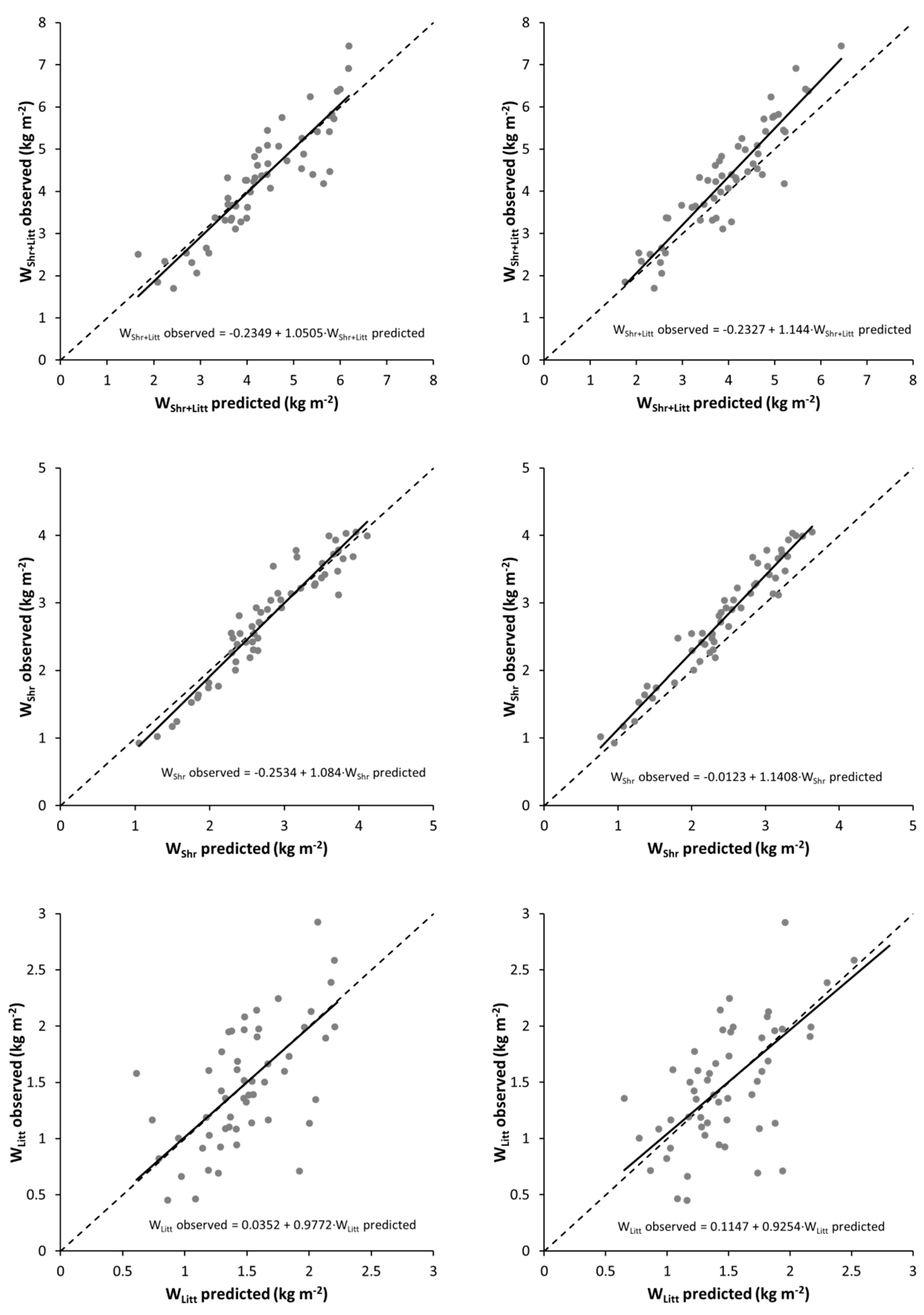
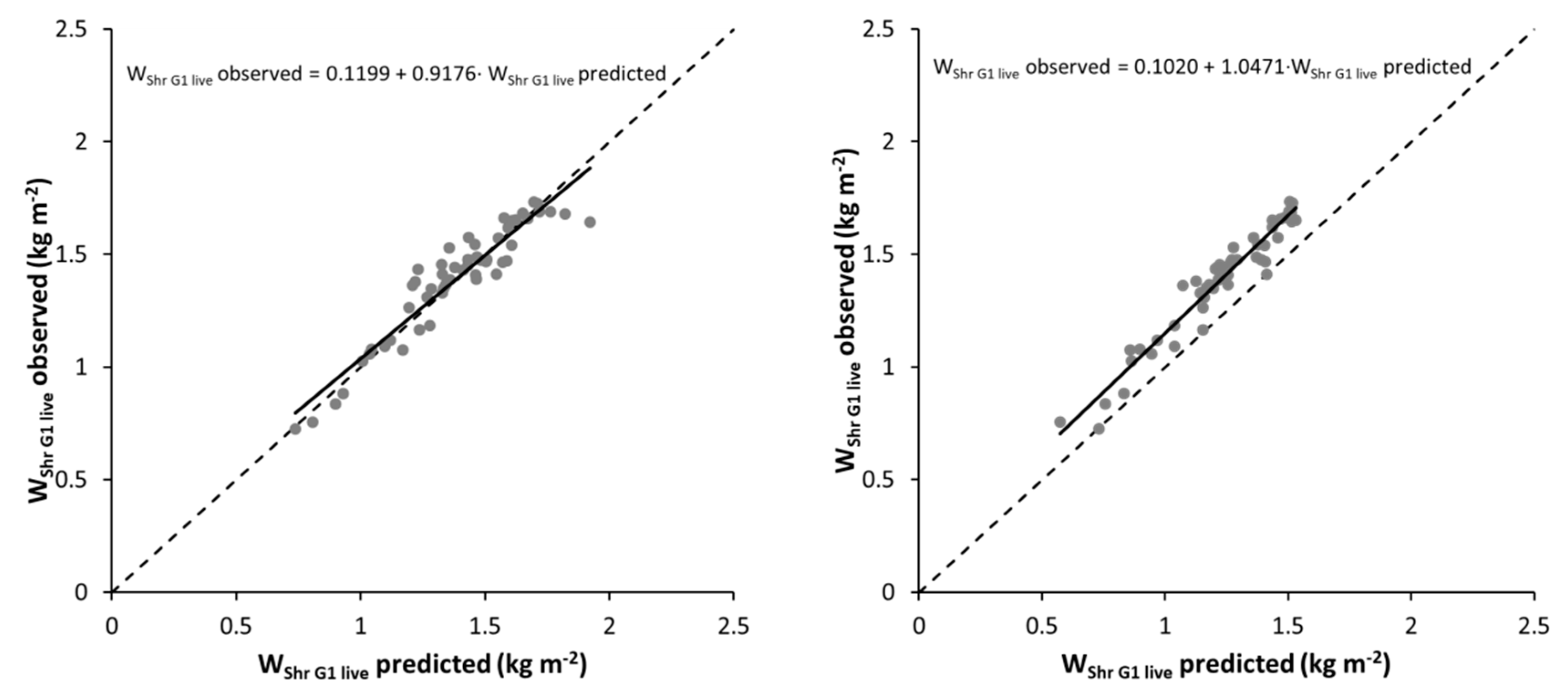
3.1. The Direct Estimation (DE) Approach

The final expressions of the system of equations fitted (Equations (1)–(7)) to the complete database of four shrub communities, including the best set of independent variables, the values of the parameter estimates, the asymptotic standard errors and the goodness-of-fit statistics, are shown in Table 4. The results of the White test and the values of the condition number did not indicate any problems of heteroscedasticity or multicollinearity for any fuel fraction.
The values and signs of all the parameters were biologically consistent and the graphical inspection of studentized residuals showed random patterns of residuals around zero, with homogeneous variance and no discernible trends. Plots of observed versus predicted values are shown in Figure 3.
All fitted equations, with the exception of the equation estimating WLitt, explained more than 80% of the observed variability, with values ranging from 80.33% to 93.92%, even exceeding 90% in the equations estimating WShr (90.18%) and WShr_G1 (93.92%). Differences between shrub communities were observed for most of the fuel fractions, except WLitt and WShr. These results are similar to those obtained by other authors. Thus, for example, the linear equations proposed by Ku et al. [82] for estimating Prosopis glandulosa biomass in rangelands in the southwestern USA yielded R2 values of 0.77–0.81 for respectively TLS-derived height bins and percentile heights as predictors; the models proposed by Olsoy et al. [43] for estimating total biomass and green biomass of individual plants of Artemisia tridentata in the sagebrush–steppe ecosystem in the western USA explained respectively 92 and 83% of the observed variability; for the same species and study area as in the aforementioned study, Li et al. [47] proposed a model that explained 87% of the observed variability; Greaves et al. [32] fitted models to estimate aboveground total biomass of low-stature (<1.5 m) Arctic shrub species in the northern Alaskan tundra, obtaining R2 values ranging from 0.91 to 0.94 depending on the scanning conditions (2 m close-range or <50 m variable-range); the linear models developed by Owers et al. [45] for estimating biomass in coastal wetland vegetation in southeast Australia explained between 42 and 99% of the observed variability, depending on the volumetric model used.
Although there are slight differences in the fitted equations, depending on the shrub community considered, the proposed system can be considered general. Because of structural and functional differences in the four communities analysed [11], improvement of the goodness-of-fit statistics is expected when a larger sample of plots to fit community-specific systems is available, especially for coarse shrub fuel load (WShr_G23), in which the inter-species variability is greater.
As previously explained, the shrub fuel loads of each fraction and community were not destructively sampled, but estimated from previously fitted equations, with CovShr, h S h r ¯ and d L i t t ¯ as independent variables. Therefore, as expected, the independent variables required as inputs to initiate the disaggregation system fitted ( W S h r + L i t t ^ equation) are TLS-based metrics related to shrub height and cover (h95 and TLSvCovShr). Three other metrics are involved in the disaggregation process: one related to the shrub height (h70) and another two related to the vertical distribution of the fuel (Wscale and IQR). The latter two variables are the only ones that discriminate between coarse and fine fuel (WShr_G23 and WShr_G1) and the categories of live and dead fine fuels (WShr_G1_live and WShr_G1_dead), highlighting the importance of the vertical distribution of fuels in the biomass loads of these fractions. Rowell et al. [44] already highlighted the importance of vertical distribution of fuels in their total load and the potential of metrics derived from the vertical height distribution of the TLS laser returns cloud for that purpose. Furthermore, the equations fitted for these fractions were also those most affected by structural differences between the four shrub communities analysed, resulting in significant community specific-parameters.

3.2. The Indirect Estimation (IE) Approach

The values of the parameter estimates, the asymptotic standard errors and the goodness-of-fit statistics for the three equations relating CovShr, h S h r ¯ and d L i t t ¯ to TLS-based metrics and variables are shown in Table 5. No problems of multicollinearity were detected for any of the three equations fitted. As expected, the best results of the goodness-of-fit statistics were obtained for h S h r ¯ , with a model explaining more than 91% of the observed variability; 66.26% for CovShr and the poorest results for d L i t t ¯ with a model explaining a 39.07% of the observed variability. Similar results were obtained in studies characterizing shrub and using TLS. Thus, e.g., Vierling et al. [37] reported values of explained variability in height and shrub cover of respectively 94 and 51%, in Artemisia tridentata dominated ecosystems in eastern Washington, USA. Anderson et al. [83] fitted models to estimate the cover fraction of shrubs (R2 = 0.77), annual grasses (R2 = 0.70), perennial grasses (R2 = 0.36), and forbs (R2 = 0.52) using the random forest algorithm in desert grasslands and big sagebrush shrublands in southwest Idaho, USA. In a study in the agro-pastoral ecotone of northern China, Xu et al. [84] proposed a model for estimating grass height and canopy cover from TLS data, which explained 70 and 72% of the observed variability respectively. Better results were obtained by Chen et al. [85], who, in a study in South-East Australia, established models for estimating the litter depth and percentage cover of the different vertical layers of the understory from TLS metrics, with R2 values of 0.9 and of 0.8–0.9, respectively.
The low accuracy of the estimates of the litter layer depth equation is consistent with the low accuracy of the estimates of the litter fuel load equation fitted in the DE approach (R2 = 0.4080). These results were expected due to the strong relationship between the litter layer depth and the accumulated load per unit area and the difficulty in characterizing this depth from the TLS point clouds because of limited visibility in high-density shrub communities [49]. Therefore, because of the importance of this fraction in both the flame and the smouldering phases, in situations in which this fraction could contribute substantially to energy flux and emissions from surface fires, destructive sampling is required to complement TLS scans.
The estimates of CovShr, h S h r ¯ and d L i t t ¯ obtained with the three models were used as inputs of the biomass equations developed for the studied communities in Galicia [69] to estimate the fuel load of WShr+Litt, WShr, WLitt, WShr_G23, WShr_G1, WShr_G1_dead, and WShr_G1_live. Plots of observed versus predicted values of these seven fuel loads are shown in Figure 3 for comparison with the same plots obtained using the DE approach.
Table 6 compares the values of R2, RMSE, bias (mean error e ¯ ), absolute bias (mean error in absolute value | e | ¯ ), and the percent RMSE (the percentage of RMSE over the mean value of the dependent variable RMSE%) from the observed and estimated fuel loads in the sample plots for each approach.
Overall, the best results, in terms of goodness-of-fit statistics, were obtained with the DE approach, although for WLitt and WShr_G23 the IE approach explained more of the observed variability, with a reduction in RMSE of, respectively, 2.6 and 13.8%, relative to the DE approach. However, the plots of observed versus predicted values showed a slight bias in all the estimates in the IE approach, with a slight tendency to underestimate the values, whereas this trend was not appreciable in the plots of the estimates of the DE approach (Figure 3).
The system of compatible equations developed with the DE approach is proposed for estimating the fuel loads of the shrub communities analyzed, with the equations fitted for the IE approach used to estimate three other important variables for complete characterization of fuelbeds (CovShr, h S h r ¯ and d L i t t ¯ ).
Apart from the important improvement regarding the provision of a compatible system of equations that guarantees additivity, the proposed methodology does not add any apparent advantages in field sampling relative to the equations based on variables obtained from non-destructive sampling, such as those already existing for the species analyzed in the study area [69]. However, as Newnham et al. [86] pointed out, TLS should not be considered just as an extension or automation of traditional field data sampling, but rather as a completely different methodology to characterize the spatial structure at the plot scale with an unprecedented level of detail. TLS point clouds can easily be processed with simple algorithms, such as those used in this study, to provide useful additional information for characterizing fuelbeds that would otherwise be difficult, impractical, or impossible to obtain with non-destructive field sampling. For example, TLS can characterize the vertical distribution of fuel loads with greater precision and at a finer scale than afforded by traditional methods (see Figure 4). Moreover, the differences in water content between green and woody biomass produce differences in reflectivity of the laser energy [87,88] enabling the TLS point cloud to be divided into green and non-green fractions [43]. In addition, previous studies have shown that TLS allows for very accurate estimates of other fundamental variables describing structural characteristics of fuelbeds, such as bulk density [49,89] or packing ratio [55]; both of which strongly influences the flammability and combustibility of a given fuelbed. For these reasons, TLS could provide improved estimates of fuelbed properties driving fire behavior, thereby enhancing the accuracy of fire behavior prediction simulators [64,65].
Several authors have highlighted the usefulness that could have the use of estimation models derived from TLS data as a stepping stone to train remote sensor databases applicable at large scale [47,48,83,90]. Therefore, the development of accurate estimation methodologies, such as those presented in this paper, based on a single TLS scan, with the consequent reduction in costs and time, constitute the basis for the application of TLS in the forest inventory, combining it with inference methods such as model-based or model-assisted approaches.
Finally, the equations proposed in this study could be useful for characterizing shrub communities from the point of view of fire behavior and fire hazard assessment, as well as for designing prescribed burns, for simulation of erosion processes, for estimating carbon stocks or biomass potential as energy source and for characterizing and delimiting wildlife habitats. Although the approach proposed is transferrable to point clouds derived from other shrub communities, new models should be fitted based on destructive sampling taking into account the specific ecosystem conditions, and considerations of timing due to phenology.

4. Conclusions

Forest managers require accurate models for estimating shrub fuel loads, especially in fire-prone areas such as Galicia, where about 2% of the forest land area is burned annually (period 1978–2019) and some two-thirds of which correspond to shrub vegetation. In this study, two alternative approaches were compared for estimating size-disaggregated shrub and litter fuel loads and live/dead fractions from TLS derived metrics, for four of the main treeless shrub communities in Galicia. The results obtained suggest that the use of metrics derived from a single TLS scan as independent variables produces accurate estimates of shrub fuel loads, mainly by using the proposed systems of equations of the DE approach.
TLS research on surface fuels is limited, and previous studies have focused on the application of physical-based fire models requiring spatially explicit three-dimensional data [49,55,63]. In addition, most of these studies have analyzed the total biomass, at best distinguishing between green and non-green fuels [43]. The proposed method therefore represents an important improvement in relation to characterization of shrub community fuel loads.
In northwest Spain, the abandonment of agricultural land, among other factors, has generated a large increase in the wildland–urban interface, creating complex mosaics in which the fire-prone shrub communities analyzed in this study predominate. Efficient management of these ecosystems increasingly demands more accurate and detailed fuel maps for comparing and prioritizing different fuel reduction strategies and ecosystem restoration. This task will require assembling and combining databases of estimates obtained from both traditional sampling and the use of remote sensors. The study findings suggest that TLS may be valuable for achieving this aim.
Our purpose is to advance towards developing a methodology that ultimately enables characterization of the spatial and vertical distribution of shrub fuels, distinguishing between size and live/dead fractions. The present research is an initial exploratory study of potentially suitable approaches to achieving these objectives. Further sampling that covers all combinations of development stages and site qualities of each shrub community, also including destructive sampling, is required to establish TLS as a robust technology for estimating the main characteristics related to fire behavior and for providing the basis for scaling up from plot to landscape.

Author Contributions

Conceptualization, C.A.-R., R.A.D.-V., and A.D.R.-G.; methodology, C.A.-R., S.A.-P., J.G.Á.-G., R.A.D.-V. and A.D.R.-G.; software, C.C., C.O. and J.G.Á.-G.; formal analysis, C.A.-R. and J.G.Á.-G.; investigation, C.A.-R., S.A.-P., J.G.Á.-G., R.A.D.-V. and A.D.R.-G.; resources, C.A.-R., S.A.-P., J.G.Á.-G., R.A.D.-V. and A.D.R.-G.; data curation, C.A.-R. and S.A.-P.; writing—original draft preparation, C.A.-R., S.A.-P., C.C., C.O., J.G.Á.-G., R.A.D.-V. and A.D.R.-G.; writing—review and editing, C.A.-R., S.A.-P., C.C., C.O., J.G.Á.-G., R.A.D.-V. and A.D.R.-G.; supervision, R.A.D.-V. and A.D.R.-G.; project administration, A.D.R.-G.; funding acquisition, A.D.R.-G. All authors have read and agreed to the published version of the manuscript.

Funding

This research was funded by the projects GEPRIF (RTA2014-00011-c06-04) and VIS4FIRE (RTA 2017-0042-C05-05) of the Spanish Ministry of Economy, Industry, and Competitiveness.

Acknowledgments

We are grateful to Mario López Fernández for his inestimable technical support in conducting all the field sampling tasks in the plot network. This work was supported by a pre-doctoral grant of the first author funded by the ‘Consejería de Educación, Universidad y Formación Profesional” and the “Consejería de Economía, Empleo e Industria” of Galician Government and the EU operational program “FSE Galicia 2014–2020”.

Conflicts of Interest

The authors declare no conflict of interest.

References

  1. Keane, R.E. Describing wildland surface fuel loading for fire management: A review of approaches, methods and systems. Int. J. Wildland Fire 2013, 22, 51–62. [Google Scholar] [CrossRef]
  2. Keane, R.E. Wildland Fuel Fundamentals and Applications; Springer International Publishing: Cham, Switzerland, 2015. [Google Scholar]
  3. Chandler, C.; Cheney, P.; Thomas, P.; Trabaud, L.; Williams, D. Fire in Forestry, Volume 1: Forest Fire Behavior and Effects; John Wiley and Sons Inc.: Hoboken, NJ, USA, 1983. [Google Scholar]
  4. Pyne, S.J.; Andrews, P.L.; Laven, R.D. Introduction to Widland Fire, 2nd ed.; John Wiley and Sons Inc.: Hoboken, NJ, USA, 1996. [Google Scholar]
  5. Finney, M.A.; Seli, R.C.; McHugh, C.W.; Ager, A.A.; Bahro, B.; Agee, J. Simulation of long-term landscape-level fuel treatment effects on large wildfires. Int. J. Wildland Fire 2007, 16, 712–727. [Google Scholar] [CrossRef] [Green Version]
  6. Ager, A.A.; Vaillant, N.M.; Finney, M.A. Integrating Fire Behavior Models and Geospatial Analysis for Wildland Fire Risk Assessment and Fuel Management Planning. J. Combust. 2011, 2011, 572452. [Google Scholar] [CrossRef] [Green Version]
  7. Jiménez, E.; Vega, J.A.; Ruiz-González, A.D.; Guijarro, M.; Alvarez-González, J.G.; Madrigal, J.; Cuiñas, P.; Hernando, C.; Fernández-Alonso, J.M. Carbon emissions and vertical pattern of canopy fuel consumption in three Pinus pinaster Ait. active crown fires in Galicia (NW Spain). Ecol. Eng. 2013, 54, 202–209. [Google Scholar] [CrossRef]
  8. Lasslop, G.; Kloster, S. Impact of fuel variability on wildfire emission estimates. Atmos. Environ. 2015, 121, 93–102. [Google Scholar] [CrossRef] [Green Version]
  9. Possell, M.; Jenkins, M.; Bell, T.L.; Adams, M.A. Emissions from prescribed fires in temperate forest in south-east Australia: Implications for carbon accounting. Biogeosciences 2015, 12, 257–268. [Google Scholar] [CrossRef] [Green Version]
  10. Restaino, J. Fuel Loading. In Encyclopedia of Wildfires and Wildland-Urban Interface (WUI) Fires; Manzello, S., Ed.; Springer: Cham, Switzerland, 2019. [Google Scholar]
  11. Arellano, S.; Vega, J.A.; Ruiz-González, A.D.; Arellano, A.; Álvarez-González, J.G.; Vega-Nieva, D.; Pérez, E. Foto-guía de Combustibles Forestales de Galicia y Comportamiento del Fuego Asociado; Andavira: Santiago de Compostela, Spain, 2017. [Google Scholar]
  12. Koutsias, N.; Allgöwer, B.; Kalabokidis, K.; Mallinis, G.; Balatsos, P.; Goldammer, J.G. Fire occurrence zoning from local to global scale in the European Mediterranean basin: Implications for multi-scale fire management and policy. iForest-Biogeosci. For. 2015, 9, 195–204. [Google Scholar] [CrossRef] [Green Version]
  13. San Miguel-Ayanz, J.; Durrant, T.; Boca, R.; Libertà, G.; Branco, A.; de Rigo, D.; Ferrari, D.; Maianti, P.; Artés Vivancos, T.; Oom, D.; et al. Forest Fires in Europe, Middle East and North Africa 2018; JRC Technical Report EUR 29856 EN: Ispra, Italy, 2019. [Google Scholar]
  14. Jiménez-Ruano, A.; Rodrigues Mimbrero, M.; de la Riva Fernández, J. Exploring spatial–temporal dynamics of fire regime features in mainland Spain. Nat. Hazards Earth Syst. Sci. 2017, 17, 1697–1711. [Google Scholar] [CrossRef] [Green Version]
  15. Rodrigues, M.; González-Hidalgo, J.C.; Peña-Angulo, D.; Jiménez-Ruano, A. Identifying wildfire-prone atmospheric circulation weather types on mainland Spain. Agric. For. Meteorol. 2019, 264, 92–103. [Google Scholar] [CrossRef]
  16. Rodrigues, M.; Trigo, R.M.; Vega-García, C.; Cardil, A. Identifying large fire weather typologies in the Iberian Peninsula. Agric. For. Meteorol. 2020, 280, 107789. [Google Scholar] [CrossRef]
  17. Xunta de Galicia. Plan de Prevención y Defensa Contra los Incendios Forestales de Galicia–PLADIGA; Consellería do Medio Rural: Santiago de Compostela, Spain, 2019. [Google Scholar]
  18. MARM. Cuarto Inventario Forestal Nacional. Galicia; Ministerio de Medio Ambiente y Medio Rural y Marino: Madrid, Spain, 2011. [Google Scholar]
  19. Catchpole, W.R.; Wheeler, C.J. Estimating plant biomass: A review of techniques. Aust. J. Ecol. 1992, 17, 121–131. [Google Scholar] [CrossRef]
  20. Bonham, C.D. Measurements for Terrestrial Vegetation, 2nd ed.; Wiley-Blackwell: Oxford, UK, 2013. [Google Scholar]
  21. Pearce, H.G.; Anderson, W.R.; Fogarty, L.G.; Todoroki, C.L.; Anderson, S.A.J. Linear mixed-effects models for estimating biomass and fuel loads in shrublands. Can. J. For. Res. 2010, 40, 2015–2026. [Google Scholar] [CrossRef]
  22. Pasalodos-Tato, M.; Ruiz-Peinado, R.; del Río, M.; Montero, G. Shrub biomass accumulation and growth rate models to quantify carbon stocks and fluxes for the Mediterranean region. Eur. J. For. Res. 2015, 134, 537–553. [Google Scholar] [CrossRef]
  23. De Cáceres, M.; Casals, P.; Gabriel, E.; Castro, X. Scaling-up individual-level allometric equations to predict stand-level fuel loading in Mediterranean shrublands. Ann. For. Sci. 2019, 76, 87. [Google Scholar] [CrossRef]
  24. Keane, R.E.; Burgan, R.; Van Wagtendonk, J. Mapping wildland fuels for fire management across multiple scales: Integrating remote sensing, GIS, and biophysical modeling. Int. J. Wildland Fire 2001, 10, 301–319. [Google Scholar] [CrossRef]
  25. Riaño, D.; Chuvieco, E.; Salas, J.; Palacios-Orueta, A.; Bastarrika, A. Generation of fuel type maps from Landsat TM images and ancillary data in Mediterranean ecosystems. Can. J. For. Res. 2002, 32, 1301–1315. [Google Scholar] [CrossRef]
  26. Reich, R.M.; Lundquist, J.E.; Bravo, V.A. Spatial models for estimating fuel loads in the Black Hills, South Dakota, USA. Int. J. Wildland Fire 2004, 13, 119–129. [Google Scholar] [CrossRef]
  27. Mutlu, M.; Popescu, S.C.; Stripling, C.; Spencer, T. Mapping surface fuel models using lidar and multispectral data fusion for fire behavior. Remote Sens. Environ. 2008, 112, 274–285. [Google Scholar] [CrossRef]
  28. Viana, H.; Aranha, J.; Lopes, D.; Cohen, W.B. Estimation of crown biomass of Pinus pinaster stands and shrubland above-ground biomass using forest inventory data, remotely sensed imagery and spatial prediction models. Ecol. Model. 2012, 226, 22–35. [Google Scholar] [CrossRef]
  29. Riaño, D.; Chuvieco, E.; Ustin, S.L.; Salas, J.; Rodríguez-Pérez, J.R.; Ribeiro, L.M.; Viegas, D.X.; Moreno, J.M.; Fernández, H. Estimation of shrub height for fuel-type mapping combining airborne LiDAR and simultaneous color infrared ortho imaging. Int. J. Wildland Fire 2007, 16, 341–348. [Google Scholar] [CrossRef] [Green Version]
  30. Estornell, J.; Ruiz, L.A.; Velázquez-Martí, B.; Fernández-Sarría, A. Estimation of shrub biomass by airborne LiDAR data in small forest stands. For. Ecol. Manag. 2011, 262, 1697–1703. [Google Scholar] [CrossRef] [Green Version]
  31. Jakubowksi, M.K.; Guo, Q.; Collins, B.; Stephens, S.; Kelly, M. Predicting Surface Fuel Models and Fuel Metrics Using Lidar and CIR Imagery in a Dense, Mountainous Forest. Photogramm. Eng. Remote Sens. 2013, 79, 37–49. [Google Scholar] [CrossRef] [Green Version]
  32. Greaves, H.E.; Vierling, L.A.; Eitel, J.U.H.; Boelman, N.T.; Magney, T.S.; Prager, C.M.; Griffin, K.L. High-resolution mapping of aboveground shrub biomass in Arctic tundra using airborne lidar and imagery. Remote Sens. Environ. 2016, 184, 361–373. [Google Scholar] [CrossRef]
  33. Li, A.; Dhakal, S.; Glenn, N.F.; Spaete, L.P.; Shinneman, D.J.; Pilliod, D.S.; Arkle, R.S.; McIlroy, S.K. Lidar aboveground vegetation biomass estimates in shrublands: Prediction, uncertainties and application to coarser scales. Remote Sens. 2017, 9, 903. [Google Scholar] [CrossRef] [Green Version]
  34. Estornell, J.; Ruiz, L.A.; Velázquez-Martí, B.; Hermosilla, T. Analysis of the factors affecting LiDAR DTM accuracy. Int. J. Digit. Earth 2011, 4, 521–538. [Google Scholar] [CrossRef] [Green Version]
  35. Glenn, N.F.; Spaete, L.P.; Sankey, T.T.; Derryberry, D.R.; Hardegree, S.P.; Mitchell, J.J. Errors in LiDAR-derived shrub height and crown area on sloped terrain. J. Arid Environ. 2011, 75, 377–382. [Google Scholar] [CrossRef]
  36. Mitchell, J.J.; Glenn, N.F.; Sankey, T.T.; Derryberry, D.R.; Anderson, M.O.; Hruska, R.C. Small-footprint LiDAR estimations of sagebrush canopy characteristics. Photogramm. Eng. Remote Sens. 2011, 77, 521–530. [Google Scholar] [CrossRef]
  37. Vierling, L.A.; Xu, Y.; Eitel, J.U.H.; Oldow, J.S. Shrub characterization using terrestrial laser scanning and implications for airborne LiDAR assessment. Can. J. Remote Sens. 2013, 38, 709–722. [Google Scholar] [CrossRef]
  38. Hopkinson, C.; Chasmer, L.; Young-Pow, C.; Treitz, P. Assessing forest metrics with a ground-based scanning lidar. Can. J. For. Res. 2004, 34, 573–583. [Google Scholar] [CrossRef] [Green Version]
  39. Astrup, R.; Ducey, M.J.; Granhus, A.; Ritter, T.; von Lüpke, N. Approaches for estimating stand-level volume using terrestrial laser scanning in a single-scan mode. Can. J. For. Res. 2014, 44, 666–676. [Google Scholar] [CrossRef]
  40. Abegg, M.; Kükenbrink, D.; Zell, J.; Schaepman, M.E.; Morsdorf, F. Terrestrial laser scanning for forest inventories—tree diameter distribution and scanner location impact on occlusion. Forests 2017, 8, 184. [Google Scholar] [CrossRef] [Green Version]
  41. Chen, S.; Feng, Z.; Chen, P.; Khan, T.U.; Lian, Y. Nondestructive Estimation of the Above-Ground Biomass of Multiple Tree Species in Boreal Forests of China Using Terrestrial Laser Scanning. Forests 2019, 10, 936. [Google Scholar] [CrossRef] [Green Version]
  42. Loudermilk, E.L.; Hiers, J.K.; O’Brien, J.J.; Mitchell, R.J.; Singhania, A.; Fernandez, J.C.; Slatton, K.C. Ground-based LIDAR: A novel approach to quantify fine-scale fuelbed characteristics. Int. J. Wildland Fire 2009, 18, 676–685. [Google Scholar] [CrossRef] [Green Version]
  43. Olsoy, P.J.; Glenn, N.F.; Clark, P.E.; Derryberry, D.R. Aboveground total and green biomass of dryland shrub derived from terrestrial laser scanning. ISPRS J. Photogramm. Remote Sens. 2014, 88, 166–173. [Google Scholar] [CrossRef] [Green Version]
  44. Rowell, E.M.; Seielstad, C.A.; Ottmar, R.D. Development and validation of fuel height models for terrestrial lidar—RxCADRE 2012. Int. J. Wildland Fire 2016, 25, 38–47. [Google Scholar] [CrossRef]
  45. Owers, C.J.; Rogers, K.; Woodroffe, C.D. Terrestrial laser scanning to quantify above-ground biomass of structurally complex coastal wetland vegetation. Estuar. Coast. Shelf Sci. 2018, 204, 164–176. [Google Scholar] [CrossRef] [Green Version]
  46. Lovell, J.L.; Jupp, D.L.B.; Culvenor, D.S.; Coops, N.C. Using airborne and ground-based ranging lidar to measure canopy structure in Australian forests. Can. J. Remote Sens. 2003, 29, 607–622. [Google Scholar] [CrossRef]
  47. Li, A.; Glenn, N.F.; Olsoy, P.J.; Mitchell, J.J.; Shrestha, R. Aboveground biomass estimates of sagebrush using terrestrial and airborne LiDAR data in a dryland ecosystem. Agric. For. Meteorol. 2015, 213, 138–147. [Google Scholar] [CrossRef]
  48. Liu, L.; Pang, Y.; Li, Z.; Si, L.; Liao, S. Combining airborne and terrestrial laser scanning technologies to measure forest understorey volume. Forests 2017, 8, 111. [Google Scholar] [CrossRef] [Green Version]
  49. Hudak, A.T.; Kato, A.; Bright, B.C.; Loudermilk, E.L.; Hawley, C.; Restaino, J.C.; Ottmar, R.D.; Prata, G.A.; Cabo, C.; Prichard, S.J.; et al. Towards spatially explicit quantification of pre- and post-fire fuels and fuel consumption from traditional and point cloud measurements. For. Sci. 2020, 66, 428–442. [Google Scholar] [CrossRef]
  50. Crespo-Peremarch, P.; Fournier, R.A.; Nguyen, V.T.; van Lier, O.R.; Ruiz, L.Á. A comparative assessment of the vertical distribution of forest components using full-waveform airborne, discrete airborne and discrete terrestrial laser scanning data. For. Ecol. Manag. 2020, 473, 118268. [Google Scholar] [CrossRef]
  51. Aicardi, I.; Dabove, P.; Lingua, A.M.; Piras, M. Integration between TLS and UAV photogrammetry techniques for forestry applications. iForest-Biogeosci. For. 2017, 10, 41–47. [Google Scholar] [CrossRef] [Green Version]
  52. Warfield, A.D.; Leon, J.X. Estimating Mangrove Forest Volume Using Terrestrial Laser Scanning and UAV-Derived Structure-from-Motion. Drones 2019, 3, 32. [Google Scholar] [CrossRef] [Green Version]
  53. LaRue, E.A.; Atkins, J.W.; Dahlin, K.; Fahey, R.; Fei, S.; Gough, C.; Hardiman, B.S. Linking Landsat to terrestrial LiDAR: Vegetation metrics of forest greenness are correlated with canopy structural complexity. Int. J. Appl. Earth Obs. Geoinf. 2018, 73, 420–427. [Google Scholar] [CrossRef]
  54. Greaves, H.E.; Vierling, L.A.; Eitel, J.U.H.; Boelman, N.T.; Troy, S.T.; Magney, T.; Prager, C.M.; Griffin, K.L. Estimating aboveground biomass and leaf area of low-stature Arctic shrubs with terrestrial LiDAR. Remote Sens. Environ. 2015, 164, 26–35. [Google Scholar] [CrossRef]
  55. Rowell, E.; Loudermilk, E.L.; Hawley, C.; Pokswinski, S.; Seielstad, C.; Queen, L.L.; O’Brien, J.J.; Hudak, A.T.; Goodrick, S.; Hiers, J.K. Coupling terrestrial laser scanning with 3D fuel biomass sampling for advancing wildland fuels characterization. For. Ecol. Manag. 2020, 462, 117945. [Google Scholar] [CrossRef]
  56. Hawley, C.M.; Loudermilk, E.L.; Rowell, E.M.; Pokswinski, S. A novel approach to fuel biomass sampling for 3D fuel characterization. MethodsX 2018, 5, 1597–1604. [Google Scholar] [CrossRef]
  57. Mandel, J.; Beezley, J.D.; Kochanski, A.K. Coupled atmosphere–wildland fire modeling with WRF 3.3 and SFIRE 2011. Geosci. Model Dev. 2011, 4, 591–610. [Google Scholar] [CrossRef] [Green Version]
  58. Mandel, J.; Amram, S.; Beezley, J.D.; Kelman, G.; Kochanski, A.K.; Kondratenko, V.Y.; Lynn, B.H.; Regev, B.; Vejmelka, M. Recent advances and applications of WRF-SFIRE. Nat. Hazards Earth Syst. Sci. 2014, 14, 2829–2845. [Google Scholar] [CrossRef] [Green Version]
  59. Mell, W.; Jenkins, M.A.; Gould, J.; Cheney, P. A physics-based approach to modeling grassland fires. Int. J. Wildland Fire 2007, 16, 1–22. [Google Scholar] [CrossRef]
  60. Mell, W.; Maranghides, A.; McDermott, R.; Manzello, S.L. Numerical simulation and experiments of burning Douglas-fir trees. Combust. Flame 2009, 156, 2023–2041. [Google Scholar] [CrossRef]
  61. Linn, R.R.; Reisner, J.; Colmann, J.J.; Winterkamp, J. Studying wildfire behavior using FIRETEC. Int. J. Wildland Fire 2002, 11, 233–246. [Google Scholar] [CrossRef]
  62. Linn, R.R.; Winterkamp, J.; Colman, J.J.; Edminster, C.; Bailey, J.D. Modeling interactions between fire and atmosphere in discrete element fuelbeds. Int. J. Wildland Fire 2005, 14, 37–48. [Google Scholar] [CrossRef] [Green Version]
  63. Hudak, A.; Prichard, S.; Keane, R.; Loudermilk, L.; Parsons, R.; Seielstad, C.; Rowell, E.; Skowronski, N. Hierarchical 3D Fuel and Consumption Maps to Support Physics-Based Fire Modeling; Joint Fire Science Program Project 16-4-01-15 Final Report; Joint Fire Science Program: Moscow, ID, USA, 2017. [Google Scholar]
  64. Finney, M.A. FARSITE: Fire Area Simulator–Model Development and Evaluation; Research Paper RMRS-RP-4 Revised; United States Department of Agriculture, Forest Service, Rocky Mountain Research Station: Ogden, UT, USA, 2004.
  65. Finney, M.A. An overview of FlamMap fire modeling capabilities. In Fuels Management—How to Measure Success, Proceedings of the Rocky Mountain Research Station, Portland, OR, USA, 28–30 March 2006; United States Department of Agriculture, Forest Service, Rocky Mountain Research Station: Fort Collins, CO, USA, 2006. [Google Scholar]
  66. MARM. Mapa Forestal de España. Escala 1:25.000; Ministerio de Agricultura, Pesca y Alimentación: Madrid, Spain, 2011.
  67. MMA. Mapa Forestal Nacional. Escala 1:50.000; Ministerio de Agricultura, Pesca y Alimentación: Madrid, Spain, 2006.
  68. Canfield, R.H. Application of the line interception method in sampling range vegetation. J. For. 1941, 39, 388–394. [Google Scholar]
  69. Arellano-Pérez, S. Modelos de Combustibles Forestales de Galicia. Master’s Thesis, Universidad de Santiago de Compostela, Lugo, Spain, 2011. [Google Scholar]
  70. Bliss, C. The Transformation of Percentages for Use in the Analysis of Variance. Ohio J. Sci. 1938, 38, 9–12. [Google Scholar]
  71. Cao, Q.V.; Burkhart, H.E.; Lemin, R.C. Diameter Distributions and Yields of Thinned Loblolly Pine Plantations; FWS 1-82; School of Forestry and Wildlife Resources, Virginia Polytechnic Institute and State University: Blacksburg, VA, USA, 1982. [Google Scholar]
  72. R Core Team. R: A Language and Environment for Statistical Computing; R Foundation for Statistical Computing: Vienna, Austria, 2020; Available online: https://www.R-project.org/ (accessed on 16 March 2020).
  73. Adler, D.; Murdoch, D.; Nenadic, O.; Urbanek, S.; Chen, M.; Gebhardt, A.; Bolker, B.; Csardi, G.; Strzelecki, A.; Senger, A. rgl: 3D Visualization Using OpenGL. R package version 0.100.54. Available online: https://CRAN.R-project.org/package=rgl (accessed on 16 March 2020).
  74. Meyer, D.; Dimitriadou, E.; Hornik, K.; Weingessel, A.; Leisch, F. e1071: Misc Functions of the Department of Statistics, Probability Theory Group (Formerly: E1071). R package version 1.7-2. Available online: https://CRAN.R-project.org/package=e1071 (accessed on 16 March 2020).
  75. Tang, S.; Li, Y.; Wang, Y. Simultaneous equations, error-invariable models, and model integration in systems ecology. Ecol. Model. 2001, 142, 285–294. [Google Scholar] [CrossRef]
  76. Tang, S.; Wang, Y. A parameter estimation program for the error-in-variable model. Ecol. Model. 2002, 156, 225–236. [Google Scholar] [CrossRef]
  77. Myers, R.H. Classical and Modern Regression with Applications, 2nd ed.; Duxbury Press: Pacific Grove, CA, USA, 1990. [Google Scholar]
  78. White, H. A heteroskedasticity-consistent covariance matrix estimator and a direct test for heteroskedasticity. Econometrica 1980, 48, 817–838. [Google Scholar] [CrossRef]
  79. Cailliez, F. Estimación del Volumen Forestal y Predicción del Rendimiento; FAO: Roma, Italy, 1980. [Google Scholar]
  80. Harvey, A.C. Estimating regression models with multiplicative heteroscedasticity. Econometrica 1976, 44, 461–465. [Google Scholar] [CrossRef]
  81. SAS Institute Inc. SAS/ETS® 9.1 User’s Guide; SAS Institute Inc.: Cary, NC, USA, 2004. [Google Scholar]
  82. Ku, N.; Popescu, S.C.; Ansley, R.J.; Perotto-Baldivieso, H.L.; Filippi, A.M. Assessment of available rangeland woody plant biomass with a terrestrial lidar system. Photogramm. Eng. Remote Sens. 2012, 78, 349–361. [Google Scholar] [CrossRef]
  83. Anderson, K.E.; Glenn, N.F.; Spaete, L.P.; Shinneman, D.J.; Pilliod, D.S.; Arkle, R.S.; McIlroy, S.K.; Derryberry, D.R. Estimating vegetation biomass and cover across large plots in shrub and grass dominated drylands using terrestrial lidar and machine learning. Ecol. Indic. 2018, 84, 793–802. [Google Scholar] [CrossRef]
  84. Xu, K.; Su, Y.; Liu, J.; Hu, T.; Jin, S.; Ma, Q.; Zhai, Q.; Wang, R.; Zhang, J.; Li, Y.; et al. Estimation of degraded grassland aboveground biomass using machine learning methods from terrestrial laser scanning data. Ecol. Indic. 2020, 108, 105747. [Google Scholar] [CrossRef]
  85. Chen, Y.; Zhu, X.; Yebra, M.; Harris, S.; Tapper, N. Strata-based forest fuel classification for wildfire hazard assessment using terrestrial LiDAR. J. Appl. Remote Sens. 2016, 10, 046025. [Google Scholar] [CrossRef] [Green Version]
  86. Newnham, G.J.; Armston, J.D.; Calders, K.; Disney, M.I.; Lovell, J.L.; Schaaf, C.B.; Strahler, A.H.; Danson, F.M. Terrestrial laser scanning for plot-scale forest measurement. Curr. For. Rep. 2015, 1, 239–251. [Google Scholar] [CrossRef] [Green Version]
  87. Gao, B. NDWI—A normalized difference water index for remote sensing of vegetation liquid water from space. Remote Sens. Environ. 1996, 58, 257–266. [Google Scholar] [CrossRef]
  88. Sims, D.A.; Gamon, J.A. Estimation of vegetation water content and photosynthetic tissue area from spectral reflectance: A comparison of indices based on liquid water and chlorophyll absorption features. Remote Sens. Environ. 2003, 84, 526–537. [Google Scholar] [CrossRef]
  89. Pimont, F.; Dupuy, J.L.; Rigolot, E.; Prat, V.; Piboule, A. Estimating Leaf Bulk Density Distribution in a Tree Canopy Using Terrestrial LiDAR and a Straightforward Calibration Procedure. Remote Sens. 2015, 7, 7995–8018. [Google Scholar] [CrossRef] [Green Version]
  90. Greaves, H.E.; Vierling, L.E.; Eitel, J.U.H.; Boelman, N.T.; Magney, T.S.; Prager, C.M.; Griffin, K.L. Applying terrestrial lidar for evaluation and calibration of airborne lidar-derived shrub biomass estimates in Arctic tundra. Remote Sens. Lett. 2017, 8, 175–184. [Google Scholar] [CrossRef]
Figure 1. Geographical location of the 55 plots in Galicia grouped in 4 shrub communities.
Remotesensing 12 03704 g001
Figure 2. Examples of sample plots with Ulex europaeus (upper) and Ulex gallii (lower) and terrestrial laser scanning (TLS)-derived laser returns cloud obtained after raw data processing.
Remotesensing 12 03704 g002
Figure 3. Plots of observed versus predicted values of shrub and litter fuel load (WShr+Litt), total shrub fuel load (WShr), litter fuel load (WLitt), coarse shrub fuel load (WShr_G23), fine shrub fuel load (WShr_G1), dead fine shrub fuel load (WShr_G1_dead), and live fine shrub fuel load (WShr_G1_live) for DE (left) and IE (right) approaches.
Remotesensing 12 03704 g003aRemotesensing 12 03704 g003bRemotesensing 12 03704 g003c
Figure 4. Vertical distribution of the relative frequency of TLS returns (a) in two fuel plots with different vertical structure (b) Ulex europaeus and (c) Ulex gallii.
Remotesensing 12 03704 g004
Table 1. Shrub community, number of plots, codes, and dominant and secondary species.
Shrub CommunityNo. of PlotsCodeDominant Shrub SpeciesSecondary Species
High heath15EaErica australis L.Pterospartum tridentatum, Halimium alyssoides (Lam.) Greuter, Erica arborea L., Ulex europaeus
Prickled broom10PtPterospartum tridentatum (L) Willk.Erica umbellata Loefle ex L., Halimium alyssoides, Erica australis L., Ulex gallii, Ulex europaeus, Pteridium aquilinum (L.) Kuhn
High gorse15UeUlex europaeus L.Ulex gallii, Erica umbellata, Pteridium aquilinum, Pterospartum tridentatum,
Low gorse15UgUlex gallii Planch./
Ulex minor Roth.
Ulex europaeus, Erica umbellata, Daboecia cantábrica (Huds.) K.Koch, Pterospartum tridentatum, Pteridium aquilinum
Table 2. Description of the main shrub and litter characteristics. Std. dev. is the standard deviation, n is the number of plots, h S h r ¯ is the mean shrub height, CovShr is the shrub cover, d L i t t ¯ is the mean litter depth, WShr_G1_dead is the dead fine shrub fuel load, WShr_G1_live is the live fine shrub fuel load, WShr_G1 is the fine shrub fuel load, WShr_G23 is the coarse shrub fuel load, WShr is the total shrub fuel load, WLitt is the litter fuel load, and WShr+Litt is the shrub and litter fuel load.
VariableStatisticEaPtUeUg
n15101515
h S h r ¯ Mean (std. dev.)84.91 (31.48)90.37 (33.94)108.18 (19.95)65.43 (21.77)
(cm)Range38.24–150.7642.86–151.0559.71–113.1013.90–109.33
CovShrMean (std. dev.)99.80 (0.52)99.34 (1.20)99.64 (0.77)98.32 (3.17)
(%)Range98.15–10096.3–10097.69–10087.5–100
d L i t t ¯ Mean (std. dev.)2.38 (1.17)4.03 (1.19)5.49 (2.11)4.56 (0.98)
(cm)Range0.78–5.602.02–5.863.08–10.552.40–5.81
WShr_G1_deadMean (std. dev.)0.41 (0.12)0.84 (0.17)0.89 (0.09)0.75 (0.18)
(kg m−2)Range0.20–0.630.58–1.010.65–1.000.20–1.00
WShr_G1_liveMean (std. dev.)1.19 (0.23)1.47 (0.25)1.40 (0.07)1.53 (0.23)
(kg m−2)Range0.76–1.531.08–1.731.18–1.480.72–1.69
WShr_G1Mean (std. dev.)1.60 (0.36)2.31 (0.42)2.29 (0.16)2.28 (0.41)
(kg m−2)Range0.96–2.161.66–2.741.83–2.470.92–2.69
WShr_G23Mean (std. dev.)0.48 (0.36)0.62 (0.40)1.17 (0.31)0.37 (0.28)
(kg m−2)Range0.06–1.380.12–1.370.46–1.580–1.09
WShrMean (std. dev.)2.08 (0.71)2.93 (0.80)3.47 (0.47)2.65 (0.63)
(kg m−2)Range1.02–3.541.77–3.992.29–4.050.93–3.78
WLittMean (std. dev.)1.00 (0.36)1.38 (0.49)1.89 (0.64)1.70 (0.35)
(kg m−2)Range0.45–1.910.71–2.251.14–3.400.93–2.14
WShr+LittMean (std. dev.)3.08 (0.99)4.31 (1.11)5.35 (1.02)4.35 (0.84)
(kg m−2)Range1.70–5.452.54–6.243.98–7.452.51–5.75
Ea = Erica australis, Pt = Pterospartium tridentatum, Ue = Ulex europaeus and Ug = Ulex gallii/Ulex minor.
Table 3. Potential independent variables related to height distribution.
MetricDescription
hmax (cm)maximum
hmean (cm)mean
hmode (cm)mode
hmedian (cm)median
hSD (cm)standard deviation
hskwskewness
hkurtkurtosis
hID (cm)interquartile distance
h01, h05, h10, h15, h20,…, h90, h95, h99 (cm)percentiles
h25 and h75 (cm)first and third quartiles
IQR (cm)Interquartile range (h75h25)
PAhmeanratio of laser returns above hmean to total laser returns
PAhmoderatio of laser returns above hmode to total laser returns
Table 4. Final expression of the system of equations fitted simultaneously to estimate fuel loads of each fraction, including the best set of independent variables, the parameter estimates, the approximate standard errors and the goodness-of-fit statistics. WShr+Litt = shrub and litter fuel load, WShr = total shrub fuel load, WLitt = litter fuel load, WShr_G23 = coarse shrub fuel load, WShr_G1 = fine shrub fuel load, WShr_G1_dead = dead fine shrub fuel load, and WShr_G1_live = live fine shrub fuel load.
EquationExpressionPar.EstimateApprox. Std. ErrorRMSE
(kg m−2)
R2
No. 1 W S h r + L i t t ^ = ( a 00 + a 01 I E a ) · h 95 a 1 · T L S v C o v S h r a 2 a000.29540.04470.57960.8033
a01−0.08600.0138
a10.64160.0351
a20.13970.0506
No. 2 W S h r ^ = W S h r + L i t t · ^ 1 1 + e x p [ b 1 · l o g ( I Q R ) + b 2 · l o g ( h 70 ) ] b10.72050.19640.26300.9018
No. 3 W L i t t ^ = W S h r + L i t t ^ · [ 1 1 1 + e x p [ b 1 · l o g ( I Q R ) + b 2 · l o g ( h 70 ) ] ] b2−0.83010.18600.45840.4080
No. 4 W S h r _ G 23 ^ = W S h r · ^ 1 1 + e x p [ c 00 + c 01 I E a P t + c 02 I U g + c 1 · l o g ( W s c a l e ) ] c004.61390.50610.19570.8263
c010.31030.0479
No. 5 W S h r _ G 1 ^ = W S h r · ^ [ 1 1 1 + e x p [ c 00 + c 01 I E a P t + c 02 I U g + c 1 · l o g ( W s c a l e ) ] ] c020.72540.08070.11540.9392
c1−0.98640.1255
No. 6 W S h r _ G 1 _ d e a d ^ = W S h r _ G 1 · ^ 1 1 + e x p [ d 00 + d 01 I E a U g + d 1 · l o g ( I Q R ) ]
W S h r _ G 1 _ l i v e ^ = W S h r _ G 1 · ^ [ 1 1 1 + e x p [ d 00 + d 01 I E a U g + d 1 · l o g ( I Q R ) ] ]
d000.91060.17770.08200.8848
d010.29000.0347
No. 7d1−0.10840.04510.08600.8794
Ij (j = Ea, Ug, Pt) = dummy variable whose value is equal to 1 for the specific community and 0 for the other shrub communities. Ea = Erica australis, Ug = Ulex gallii/ Ulex minor, Pt = Pterospartum tridentatum. h95 = 95th percentile height of laser returns (cm); TLSvCovShr = ratio between the observed number of laser returns and lrmax_ver; IQR = Interquartile range (h75h25) (cm); h70 = 70th percentile height of laser returns (cm); Wscale = scale parameter of the Weibull pdf.
Table 5. Final expression of the equations fitted to estimate the inputs of the biomass equations developed for the shrub communities in Galicia [69] from usual field measurements, with TLS-based metrics, the parameter estimates, the approximate standard errors and the goodness-of-fit statistics. CovShr = shrub cover (%), h S h r ¯ = mean shrub height and d L i t t ¯ = mean litter depth.
VariableExpressionPar.EstimateApprox. Std. ErrorRMSER2
CovShr (%) C o v S h r ^ = 100 1 + e x p ( a 0 + a 1 · h 95 ) a0−0.47420.17071.1226%0.6626
a1−0.09670.0145
h S h r ¯ (cm) h S h r ¯ = b 0 + b 1 · h m a x + b 2 · h 10 b0−9.89584.24589.2027 cm0.9175
b10.80800.0430
b22.57620.5859
d L i t t ¯ (cm) d L i t t ¯ = c 0 + c 1 · h k u r t +
+ c 2 · T L S v C o v S h r + c 3 · I Q R
c0−2.81561.24221.5190 cm0.3907
c11.93380.9432
c27.96322.0776
c30.10610.0204
h95 = 95th percentile height of laser returns (cm); hmax = maximum height of laser returns (cm); h10 = 10th percentile height of laser returns (cm); hkurt = height of laser returns corresponding to kurtosis; TLSvCovShr = ratio between the observed number of laser returns and lrmax_ver; IQR = Interquartile range (h75h25) (cm).
Table 6. Goodness-of-fit statistics obtained with the direct estimation (DE) and indirect estimation (IE) approaches for each fuel fraction.
VariableDirect Estimation (DE) ApproachIndirect Estimation (IE) Approach
R2RMSE
(kg m−2)
e ¯ | e | ¯ RMSE
(%)
R2RMSE
(kg m−2)
e ¯ | e | ¯ RMSE
(%)
WShr+Litt0.80330.5796−0.01830.448913.580.76420.63470.33390.524214.87
WShr0.90180.2630−0.01930.21219.500.76660.40560.33080.339314.65
WLitt0.40800.45840.00100.357230.550.43780.44670.00310.348229.78
WShr_G230.82630.1957−0.01600.144029.510.87100.16870.08880.123525.44
WShr_G10.93920.1154−0.00320.09585.480.67320.26760.24200.244412.71
WShr_G1_dead0.88480.0820−0.00900.065411.470.83710.09750.08210.084413.63
WShr_G1_live0.87940.08600.00580.06406.190.51030.17340.15990.160212.47
Publisher’s Note: MDPI stays neutral with regard to jurisdictional claims in published maps and institutional affiliations.

