Tangle-Free Exploration with a Tethered Mobile Robot


Department of Mechanical and Aerospace Engineering, Statler College of Engineering and Mineral Resources, West Virginia University, 1306 Evansdale Drive, Morgantown, WV 26506-6070, USA
*
Author to whom correspondence should be addressed.
Remote Sens. 2020, 12(23), 3858; https://0-doi-org.brum.beds.ac.uk/10.3390/rs12233858
Submission received: 16 October 2020
/
Revised: 9 November 2020
/
Accepted: 23 November 2020
/
Published: 25 November 2020
Abstract
:Exploration and remote sensing with mobile robots is a well known field of research, but current solutions cannot be directly applied for tethered robots. In some applications, tethers may be very important to provide power or allow communication with the robot. This paper presents an exploration algorithm that guarantees complete exploration of arbitrary environments within the length constraint of the tether, while keeping the tether tangle-free at all times. While we also propose a generalized algorithm that can be used with several exploration strategies, our implementation uses a modified frontier-based exploration approach, where the robot chooses its next goal in the frontier between explored and unexplored regions of the environment. The basic idea of the algorithm is to keep an estimate of the tether configuration, including length and homotopy, and decide the next robot path based on the difference between the current tether length and the shortest tether length at the next goal position. Our algorithm is provable correct and was tested and evaluated using both simulations and real-world experiments.

1. Introduction
Several recent works have considered applying autonomous mobile robots for remote sensing and exploration of unknown and/or dangerous environments [1,2,3]. Unknown environment exploration is a standard problem in mobile robotics and is fundamental for a lot of applications. Exploration is often performed by robots equipped with sensors that range from cameras and sonars to high-end LiDARs. The goal of such exploration platforms is usually to create a map of the environment where the mobile robot is placed into. Assuming that the environment is partially or entirely unknown and the mobile robot platform is autonomous, simultaneous localization and mapping (SLAM) approaches are generally used during the exploration, as continuous and accurate robot localization is essential for building a precise map of the environment [4].
Autonomous robotic exploration is a well-developed field of research, with strategies ranging from simple frontier-based exploration [5] and graph-based methods [6] to more sophisticated techniques, such as potential information fields [7] and the use of harmonic functions [8]. The basic idea of most methods is to increase the current information the robot has about the environment. An interesting approach that explicitly maximizes the information is [9]. The authors use a laser scanner to construct an Occupancy Grid model [10] of their environment and an EKF algorithm for their SLAM implementation. The exploration approach presented in this paper was implemented using the frontier-based method for goal selection. In this method, the robot selects its next goal at the border between known and unknown space. However, the general algorithm we are proposing is not limited to only this approach and any exploration method can be used for goal selection.
Considering that all untethered mobile robots require an on-board power source, energy conservation becomes a big concern for prolonged missions. To address this problem, the authors of [11] have developed an energy-efficient exploration algorithm that reduces the energy consumption of the robot by selecting consequent goals in a way that minimizes repeated coverage of the already mapped area. Such an approach therefore also results in a minimized global path length, a criterion that we will also be aiming to achieve with our approach.
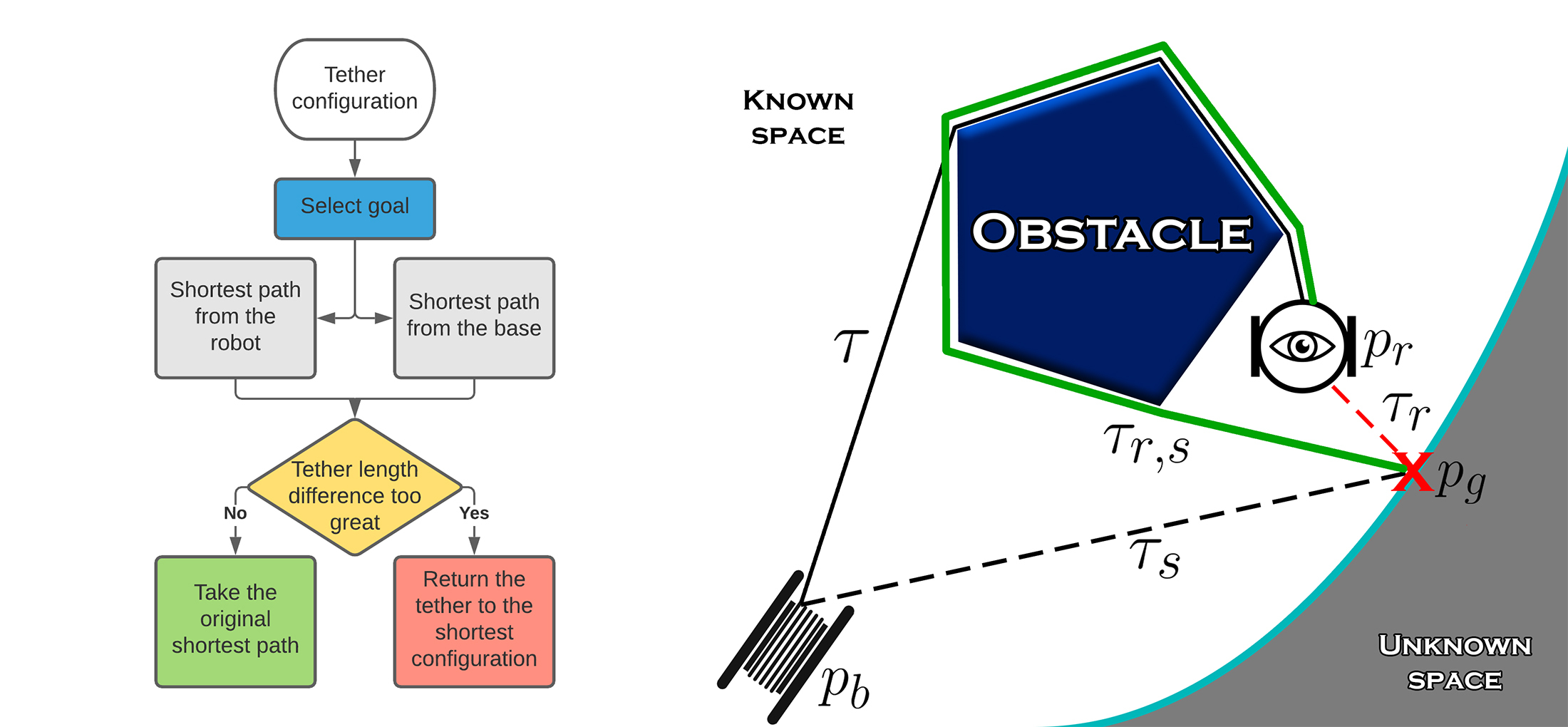
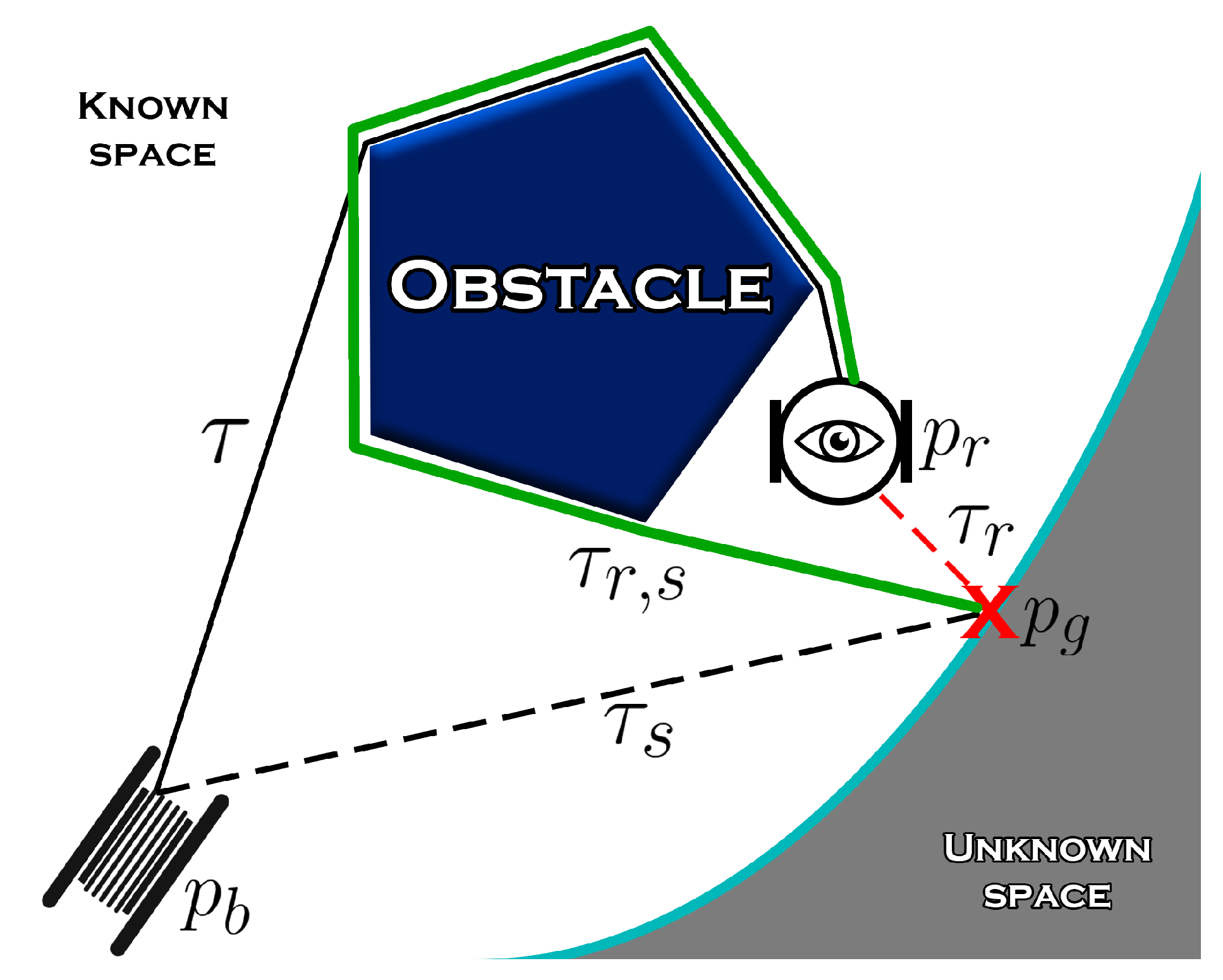
The exploration approaches mentioned above assume a freely moving untethered robot. There can be several motivations for using a tethered robot for exploration and remote sensing. Not only could the tether be used as an anchor for navigating a steep and otherwise inaccessible terrain [12], but it could also serve as a high-speed low-latency data connection to the robot in an environment where wireless communication would be problematic, like underground mines or deep underwater [13]. In addition to data, the tether could also provide power to the robot, reducing its overall weight and allowing prolonged mission time, by eliminating the need for on-board batteries. The main problem created by a tether, especially in environments with a large number of obstacles, is avoiding the tangling of the tether around the obstacles. Presenting a solution to this problem is the goal of this paper. An illustration of our proposed solution is shown in Figure 1, where we the robot chooses to take a longer path to avoid tangling its tether around the obstacle.
The use of tethered robots for space applications has been considered in [14]. The ROSA rover described in the paper uses a 40 m tether system both as a power supply and a communication link to the main platform. This reduces the weight of the rover that can in turn be used to carry more scientific instruments. The sensors on the tether in combination with a camera on the base platform are also used as a tracking mechanism. The tangling problem was not yet solved in the paper. Another application of a tethered robot for exploration has been extensively discussed in [15]. The author discusses using a tethered robot for exploring extremely steep terrains. Contrary to our solution, during the exploration, the tether gets intentionally wrapped around the obstacles to serve as additional anchor points, which then gets subsequently unwrapped on the robot’s return trajectory.
In order to achieve tangle-free exploration, the robot’s path planning algorithm should not only be intelligent enough to account for the tether, but also make decisions that would keep the tether at its shortest possible length for a given configuration. One of the ways to keep track of the tether configuration is using the notion of homotopy. Two tether configurations are said to be within the same homotopy class (i.e., homotopic to each other) if they can be continuously deformed into each other without intersecting an obstacle. It is worth noting that there are several published homotopic path planners. One example is [16], in which the authors have successfully developed a planner that gets a robot to the goal while considering the cable length and its interaction with the obstacles in the environment. Their approach, however, uses only the distance from the initial vertex to distinguish between homotopy classes, which may fail in scenarios where the same distance can represent multiple configurations. This concept was later expanded by the authors of [17]. Instead of using a single metric like the distance, they propose the use of true homotopy invariants, with each possible configuration having its own unique h-signature. A homotopy augmented graph (or h-augmented graph as called by the authors) is then used by the authors to plan tangle-free point-to-point paths.
Some homotopic planners are sampling-based algorithms based on the Rapidly-exploring Random Tree (RRT) [18] or its asymptotically optimal version, RRT*. Examples of these include H-RRT [19], which partitions the search space in order to constrain the sampling regions, HARRT* [20], which can achieve asymptotic optimality of a generated path within a given homotopy class, and a homotopy-aware kinodynamic planner [21] that proposes an approach that can consider the differential constraints of the robot. Another example of a homotopic path planner is a topology-based multi-heuristic A* [22]. It should be noted that while all the methods mentioned above can successfully generate a path in a given homotopy class, they all rely on the complete knowledge of the environment, which makes their direct use in an exploration scenario challenging.
Although we did not find a previous work (with the exception of our own conference paper [23]) that solves the tethered exploration problem, tethered coverage, which is a very similar problem, has been solved in [24]. The authors successfully developed an algorithm that uses a tethered robot to fully cover an arbitrary unknown environment, while also keeping the tether in a tangle-free state. This work has later been expanded in [25]. This paper proposes an algorithm for tethered coverage that successfully minimizes the total path length required to cover the unknown environment. However, because the path required to completely explore the environment is generally far smaller than the path required to cover one, especially with long-range sensors, direct use of these approaches for exploration may not be the best solution.
Thus, based on the author’s knowledge, our previous conference paper [23] is the first one that directly addresses the tangle-free exploration problem with tethered robots. While our previous work did solve the same problem considered in the current paper, there are several key differences and improvements in this paper:
- The main algorithm has been generalized and made modular, meaning it is no longer limited neither to frontier-based exploration, which we used in the previous paper, nor to any specific path planner.
- A new path planning algorithm is proposed and implemented, resulting in much better performance.
- Our current implementation is fully integrated with SLAM. Differently from [23], which assumed that the position of the robot was known, the system is now completely independent of any external tracking device, allowing autonomous exploration with the on-board sensors only.
- New simulations and real-robot experiments are performed to evaluate and illustrate our approach.
The rest of the paper is divided as follows. Section 2 presents a clear definition of the problem we are trying to solve. Section 3 presents a background on homotopy and h-signatures, which are used in our approach. Section 4 describes and analyzes the proposed approach. The results of our simulations and real-world experiments are presented in Section 5. Finally, Section 6 presents the conclusions and possibilities of continuity.
2. Problem Definition
This section defines the problem solved in this paper. Consider an unknown, planar environment populated with a number of unknown random obstacles of arbitrary shape and size. Exploration, which we consider to be the task of maximizing the information about the environment to construct a map, is to be done with a planar robot, tethered to the fixed base at position . The robot is expected to start the exploration at the position of the base . We assume that the tether is able to freely rotate around the robot, meaning the rotation of the robot will not cause the tether to be wound up around the robot itself. The tether is assumed to be retractile and always kept in a taut condition, and the maximum tether length must not be exceeded at any point during the exploration. Our goal is to efficiently cover and map the maximum amount of ground with the footprint of the robot’s sensor, which in our case is assumed to be a circle with the radius equal to the field of view of the sensor, while making sure that the tether is kept in a tangle-free configuration at all times. With the tether constraints in mind, it is also possible for the robot to not be able to reach some parts of the environment, in which case the robot should still be able to explore any and all the parts that it can reach.
As briefly mentioned in the previous section and illustrated in Figure 1, we propose an exploration algorithm that would guarantee that the tether would be kept in a tangle-free state throughout the entire exploration process. This is achieved by keeping track of the tether configuration and not allowing the robot to stray too far from the optimal global tether configuration. However, first, it is important to mention how we define tangling, as this definition will be used as the basis for our approach.
Definition 1
(Tangling). Consider a tethered robot in a planar environment with tether represented by , , where is the position of the base and the position of the tether’s attachment to the robot. If there exist points and along the tether such that and , the tether is considered to be tangled.
In other words, any taut tether configuration that loops around the obstacles and crosses itself is defined as tangled. However, especially in particularly dense environments, the tether could also get wound up around multiple obstacles in sequence without actually tangling as per Definition 1 but still resulting in a configuration that is very far from the optimum. The algorithm we are proposing eliminates such configurations from the solution space as well.
3. Background on Homotopy
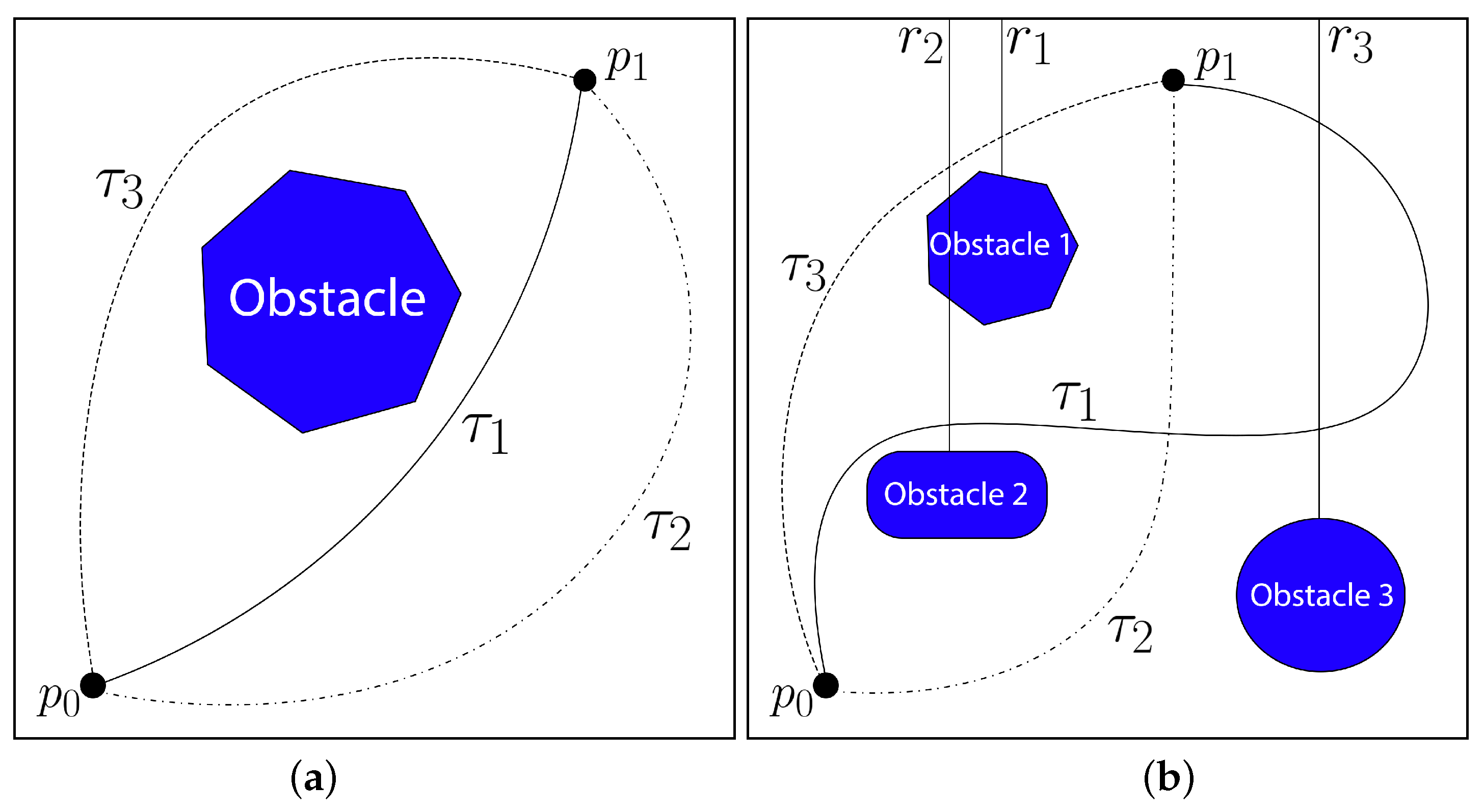
Considering the topological nature of the posed path planning problem, it is important to explain the notion of homotopy in that context and describe the way we will be using it. In essence, two paths that start and finish in the same configuration are considered to be homotopic to each other if they can be continuously deformed into each other without crossing any obstacles. Two homotopic paths are said to be in the same homotopy class, which is represented by a unique invariant called h-signature [17]. Examples of homotopic and non-homotopic paths are shown in Figure 2a—paths and are homotopic to each other and therefore have the same h-signature, i.e., , where h is a function that computes the homotopy class of a given path. In Figure 2a, path cannot be deformed into without crossing the obstacle, indicating that they are not homotopic and, therefore, do not belong to same homotopy class, i.e., . In the context of path planning for tethered robots, homotopy is an important concept. If, for example, a robot equipped with a retractile tether anchored in follows the path of Figure 2a, its tether would assume a shape that is homotopic to . The taut tether would have the same shape if the robot follows , which is also homotopic to , as we concluded earlier. Therefore, by constraining the path of the robot to have a specific homotopy class, we can constrain the tether to have the same class. The idea of this paper is to plan robot paths that make the tether to be homotopic to the shortest possible path from the anchor position to the goal. Since the shortest path, by definition, does not circulate any obstacles, the tether will also not circulate an obstacle, thus guaranteeing a tangle-free motion.
As proposed in [17], the h-signatures themselves are defined by the rays emanating vertically from the obstacles, and are computed for a path by the order those rays are crossed in. An example is shown in Figure 2b. It is important to notice that, if a ray is crossed backwards, meaning right to left, a “−1” superscript is added to that particular signature. For example, the h-signature of path shown in Figure 2b would be if the path is taken from to , but, if the same path were to be taken from to , the h-signature would now be . This is also called inverting the h-signature of a path, so, in this example, . Another important property of h-signatures is that the same ray crossed back and forth in sequence cancels out. An example of this is path , whose h-signature would originally be , but, because was crossed back and forth in sequence, its signature cancels out leaving the overall h-signature of as just . Such distinction will be important for getting the approximate tether configuration from the total path taken by the robot.
Lastly, it is important to note how it is possible to concatenate h-signatures of two different paths. Suppose we have two paths and , and the end of coincides with the start of . For such paths, it is possible to get the overall h-signature , with “◊” being the concatenation operator.
4. Exploration Algorithm
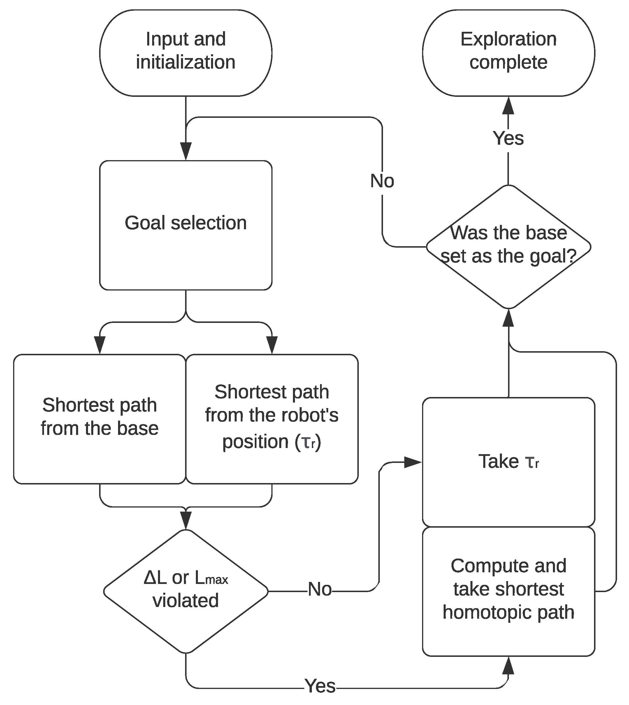
This section presents the main algorithm proposed in this paper. Figure 3 shows a flowchart for the generalized algorithm we are proposing. The key parameter in the algorithm, which will be responsible for keeping the tether tangle-free, is the length tolerance . This parameter is a comparison between the shortest path from the base to the goal and the tether configuration if the robot were to take the shortest path from its current position to the goal. This tolerance is used to determine whether the robot should take the shortest path to the goal or take the path that would put it in the same homotopy configuration as the shortest path from the base.
Algorithm 1 presents a more detailed algorithmic version of the flowchart shown in Figure 3. The algorithm is initialized with the position of the tether anchor (i.e., robot base) , maximum allowed tether length , and the length tolerance . The total path is initialized as an empty set before the exploration begins. The position of the robot , the free space and the obstacle positions are expected to be dynamically updated via SLAM in parallel with the main algorithm.
| Algorithm 1 Tether-aware exploration algorithm, general form. |
 |
The algorithm itself can be thought of as having different modules that can be replaced with any desired approach. The first such module is goal selection at line 5, which will depend on the exploration approach used in the algorithm. The second, shortest path planning module would then first compute the shortest path from the base to the goal (line 10), and then the shortest path from the robot to the goal (line 11). Line 12 is the main contribution of this algorithm, and it is what is responsible for keeping the tether in a tangle-free configuration. Using the function L to get the estimate of the taut tether configuration in a given path, the algorithm checks both if the difference between the tether configuration if the robot were to take the shortest path and the optimal configuration in exceeds the length tolerance , and if the total path should the robot take the path exceeds the maximum tether length . If any one of those two conditions is violated, on line 13, the algorithm then proceeds to compute the h-signature required to put the robot back in the shortest possible tether configuration. This h-signature would be the same as backtracking to the base and then taking the shortest path . Notice that the robot will not actually backtrack all the way to the base. Lastly, the third module is the homotopic path planner (line 14) that computes the shortest path from the robot position to the goal satisfying a unique h-signature computed in the previous step. Note that this path replaces computed in line 11. Finally, line 16 commands the robot to take the computed path . This path is subsequently added to the total path record in line 17.
When the algorithm runs out of available goals to select (line 6), either by completely exploring the environment or by no longer having any goals that can be physically reached with the tether constraint , the algorithm concludes the exploration process by selecting the base as the final goal and subsequently returning to it. This process is shown in lines 6 through 9.
4.1. Analysis
By properly selecting the length tolerance , the algorithm will guarantee to always keep the tether in a tangle-free configuration by returning to the optimal shortest configuration before the tether has a chance to tangle. However, it is important to discuss a theoretical upper limit on beyond which a tangle-free global path is no longer fully guaranteed. This upper limit is demonstrated in Theorem 1.
Theorem 1.
Algorithm 1 guarantees tangle-free paths if the length tolerance is smaller or equal to the circumference of the smallest expected obstacle in the robot’s configuration space.
Proof.
Using Definition 1 for tangling and a circular obstacle as an example, the only way a taut tether can cross itself is by looping around the obstacle. The shortest possible way to loop the tether around a circular obstacle so that is by encircling the obstacle completely, giving the smallest tangle radius as , where R is the radius of the smallest obstacle. □
Theorem 1 states that the maximum allowed tolerance value would be . In the real world, however, the robot would rarely be expected to perfectly encircle an obstacle during the exploration. Thus, depending on the complexity of the environment and density of the obstacles, it is generally safe to pick values for slightly larger than the theoretical maximum of . This will be supported by our simulation results in Section 5.1.
4.2. Implementation
It is important to mention that, since Algorithm 1 is generalized, an implementation of that algorithm will not always follow strictly the same structure. Our implementation shown in Algorithm 2 uses a modified frontier-based exploration method for the goal selection module and algorithm as the shortest path planner, but the homotopic path planning and goal selection modules are not as clearly separated as they are in Algorithm 1. We are also using a path optimizer instead of a traditional path planner to get the homotopic shortest path. The reasons and the algorithm for this will be explained in Section 4.3.
| Algorithm 2 Implemented tether-aware exploration algorithm. |
 |
At its core, Algorithm 2 still uses a similar structure to Algorithm 1, with the exception that the goal selection and path acquisition modules (lines 5–15 in Algorithm 1) are now meshed together. Before the exploration begins, the algorithm initializes the total path array as an empty set in line 1, and requests the robot position , free space , obstacles and frontier to be updated dynamically in real time through the connected SLAM system. This algorithm uses a frontier-based exploration method as the basis for the goal selection. The main modification in our algorithm is that it samples multiple goal points and then picks the most cost-effective goal to follow, with the cost defined by the length of the path required to reach that goal with the tether constraints accounted for. If the final tether configuration of a proposed path will result in the tether length exceeding the maximum allowed value of , the cost for that path is set to ∞, signifying that this particular path would be impossible to take.
At the beginning of each cycle of the main loop, both the list of proposed paths and the list of their associated costs are defined (re-defined in the following cycles) as empty sets in line 5. In lines 6 through 9, the algorithm attempts to find the frontier that is closest to the base that could also be physically reached with the tether length constraint. The loop keeps iterating until it either finds the closest frontier cell that the tether could physically reach or runs out of frontier cells to sample (line 9). The function used to compute both the paths and their respective costs is shown in Algorithm 3 and will be explained later. Lines 10 and 11 execute a similar process, except only the closest frontier cell to the robot is tested. Lastly, lines 12 through 15 pick a number of random frontier cells to test, with the exact number defined by the input variable , which in our experiments has been set to eight random cells, giving a total of 10 cells to sample assuming the cell in lines 6–9 is found immediately. By testing both the closest frontier to the robot and the closest frontier to the base, as well as sampling several cells across the entire frontier, the algorithm ensures that the total path length is kept to a minimum throughout the exploration process.
Overall, lines 5 through 15 can be seen as both the goal selection module and the path generation module of Algorithm 1. Line 16 then checks if the algorithm has no more frontiers to sample or if all the sampled frontiers are impossible to reach, in which case the final goal is selected as the base in line 17 and the path is generated to take the robot there, after which the exploration concludes. Otherwise, in line 21, the algorithm picks the cheapest path that it could take out of all the earlier tested frontiers. Lastly, line 23 commands the robot to take the selected path, and line 24 adds that path to the total path array.
An important point to mention is that, in our implementation, we decided to use simple Euclidean distance to get the closest frontiers instead of a true path length that would be required to get there in order to save on computation time. While it could be argued that using a true path length instead of Euclidean distance would result in a more optimal goal selection and therefore shorter total path length required to explore the environment, in our simulations, when we compared the algorithm with Euclidean distance sorting versus the true distance sorting, we did not see a measurable difference in total path length.
Lastly, the function shown in Algorithm 3 is the actual core of our approach that guarantees global tangle-free paths. As described in Algorithm 1 earlier, lines 1 and 2 of Algorithm 3 generate the shortest paths to the goal from the base and from the robot respectively, which in our implementation is done by the algorithm, which assumes that the environment is represented by a grid. Line 3 here serves the same function as line 12 in Algorithm 1, in that it checks if the tether length should the robot take the path from line 2 is greater than the most optimal tether configuration from a path acquired in line 1 by more than the length tolerance , and if that same length should the robot take the path would be greater than the maximum tether length . Should any of these conditions be violated, in lines 4 and 5, the algorithm generates the shortest path that would take the robot to the optimal tether configuration that would have the same homotopy as if the robot would have returned to the base and then took the shortest path . Note that this is no longer a proper path planner, but a path optimizer, which will be further explained in the next subsection. Should the newly generated path in line 5 still result in the tether length being greater than , a condition that is checked in line 7, this would mean that the goal in question is impossible to reach with the imposed tether length limit, and the cost for that path is set to ∞ in line 8. Otherwise, in line 10, the cost is set to the length of the path computed earlier.
| Algorithm 3 “GetPath” function. |
 |
4.3. Homotopic Path Optimizer
Considering the h-signature of the return path in our approach is always the same as if the robot would backtrack to the base and subsequently take the shortest path to the goal (i.e., line 13 in Algorithm 1), we found that, instead of planning a homotopy-constrained path, it would be much simpler to add the shortest path to the inverse of the total path (line 4 in Algorithm 3), and then optimize the resulting path while keeping its h-signature unchanged. The optimizer we are using is a simple 2-step process of first shortening the path by removing the extraneous nodes as shown in Algorithm 4, and then subsequently tightening the resulting path to get it closer to the obstacles without colliding, as shown in Algorithm 5. While this approach will not result in the shortest path possible, we have empirically observed that the length difference between the optimized path and the shortest one is negligible. In addition, optimizing the path has proven to be much more computationally efficient than computing the shortest path.
| Algorithm 4 OptimizeShort algorithm. |
 |
| Algorithm 5 OptimizeTight algorithm. |
 |
Algorithm 4 is a traditional path shortening algorithm [26]. It works by first trying to directly connect the first and last nodes of the input path, and the criteria for a successful connection is for the new path to be both collision-free and have the same h-signature as the original path (line 6). Should that fail, the algorithm then tries to connect the first node to the second-to-last node and so on until it either succeeds or the ending node comes all the way down to the starting node (line 12), at which point the starting node is moved up by one and the ending node is set to the last node again. This cycle continues until the start node comes all the way up to the end (line 4).
The shorter path optimized in Algorithm 4 is then fed into Algorithm 5 to be further optimized by making that path tighter. This algorithm goes through every node in the path except the first and last ones (line 1). The node that is being currently manipulated is first moved along the line on the path “downstream” from it as far as it can go without resulting in collisions (lines 2 through 4). The same node then undergoes a similar process, now moving it along the line on the path “upstream” from it (lines 5 through 7). This process results in a final path with minimal space wasted between the obstacles.
5. Results
The approach that we proposed in Algorithm 2 has been implemented using Python programming language and the ROS (Robot Operating System) framework [27]. We used as our SLAM system and have tested the implementation both in simulations and using a real-world robot.
5.1. Simulations
In order to test our algorithm’s both statistical and real-world performance before implementing it on a real robot, we first implemented the algorithm in a stand-alone Python environment to isolate all the external variables and focus on the algorithm itself. The core algorithm is unchanged in this implementation, but both the robot movement and localization are removed from the calculations and are just supplied to the algorithm in a perfect form. Mapping is also being simulated with a separate function that emulates a sensor reading in a given field of view, with its own computation time excluded from the statistical records. Because both localization and mapping in a full implementation are performed in parallel via SLAM, this approach is still representative of the performance of the algorithm. Gazebo [28] simulations were also performed. These simulations used a full implementation of the algorithm, with both and proper robot movement.
5.1.1. Performance Metrics
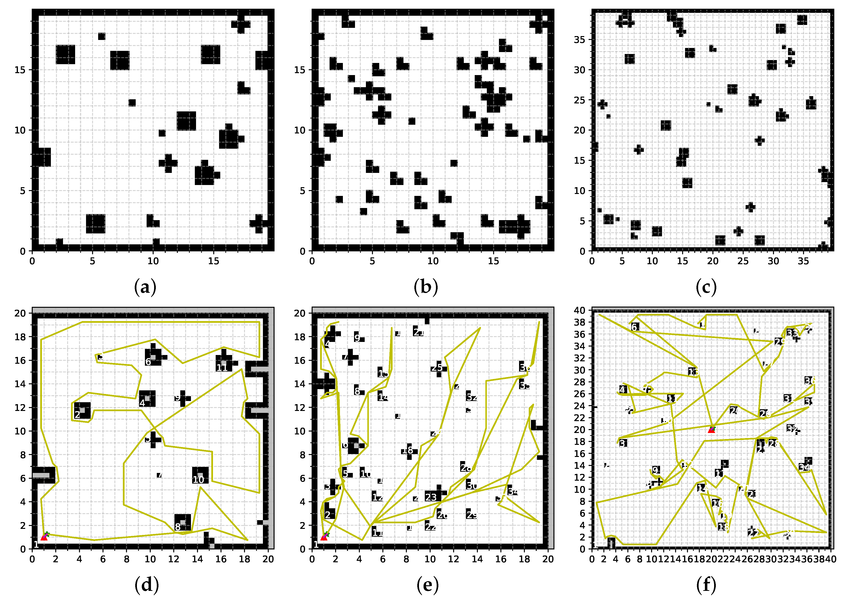
To make sure the algorithm gets properly tested in various scenarios, we prepared three randomized environment types to run the algorithm against, all of which were run with a resolution of and the maximum tether length set to 40. Typical configurations of these environments as well as example paths taken to explore them are demonstrated in Figure 4. We do not specify any units in these simulations since, for measuring the performance of the system, a map with a resolution of would be computationally identical to a map with a resolution of 1, assuming the field of view and the maximum tether length are also scaled appropriately. However, one can assume that all dimensions are in meters, since the same approach is also translated to both the Gazebo simulations and the real-world experiment.
The first “low-density” environment type in Figure 4 is a 20 × 20 map with 15–20 random obstacles, each of radius up to 2. The second “high-density” environment type is also a 20 × 20 map, but now with 50–60 random obstacles, each of radius up to 0.5. Lastly, the third “large” environment type is a 40 × 40 map with 40–50 random obstacles, each of radius up to 2. The field of view of the simulated sensor was set to 4 for both low and high-density environments, and 10 for large environments. Due to the random nature of this approach, the actual number of discrete obstacles on a given map is generally less than the defined value due to obstacle overlap.
All the environment types mentioned above were simulated with varying length tolerances to observe the effect it has on tangling rate, computation time, number of iterations it took to explore a given environment, maximum reached tether length, and total path length required to explore the environment. In addition to that, two extra simulations were performed as control samples—one that avoided tangling by simply backtracking the robot to the base after every iteration before selecting the next goal, and one with the tether length constraint removed to represent the standard frontier-based approach. The simulations were performed 50 times per value of to get a representation of average performance that should be expected from a given configuration. All of this was run on an AMD RyzenTM 9 3950x CPU on a machine running Windows 10. The CPU’s reported clock speed during the simulations was 4.2 GHz.
The results from simulations of the low-density environment type are shown in Table 1. There are several important trends in this table that are worth pointing out. First of all, as we have proved, the length tolerance did indeed result in a tangle-free global path every time. However, since this environment type was not densely populated with obstacles, the value of also resulted in tangle-free global paths, supporting our claim that depending on the environment type, values of slightly larger than will generally be fine. Beyond that, however, we start to see progressively more tangling the larger becomes. As expected, the largest tangle percentage was acquired for a simulation type where restrictions on the tether length were removed as well. The shortest maximum tether reached is, as expected, achieved with simple backtracking, and the longest one is where the tether limit was removed. For the simulations with varying , we see an increasing trend, with the maximum tether length leveling off to as . While the average amount of iterations required to complete one map are all within the margin of error of each other for every simulation parameter with a slight increasing trend (with the exception of “Backtrack” simulation), computation time per iteration is measurably increasing with , and the total time also increases as a result. This can be explained by the robot straying progressively further from the optimal tether configuration with larger values of , which in turn requires the path optimizer to work with more complex h-signatures, thus increasing the overall computation time. Lastly, there are several interesting points regarding the total path length taken by the robot. The shortest one is, as expected, the one where both and the tether length were ignored, and the longest one is when the robot used simple backtracking, resulting in the path length almost 10 times the former. As for the simulations with varying , we can see that the longest path was for , with the minimum being achieved somewhere around . The value of would force the algorithm to always return to the shortest tether configuration, and while this does guarantee a tangle-free global path, this approach is not the most efficient, hence the increased total path length. On the other hand, even if we ignore tangling, increasing too much would allow the robot to stray too far from the optimal configuration, which in turn would require a longer return path to get back to the optimum, resulting in a longer global path again. The minimum total path length is reached in between these two extremes.
It should be noted that the tangle detection function is only able to return a positive detection based on Definition 1 of tangling. This is why even with the tangling percentage is not nearing 100%, even though the tether may be wound up around multiple obstacles and very far from the optimal configuration. This will be important to keep in mind for the high-density environment results.
Results for a high-density environment demonstrated in Table 2 show a similar picture, but there are a few key differences. First of all, with the environment being a lot more tightly packed with obstacles, tangle percent for is no longer zero, while still guarantees a tangle-free global path, with a slightly more aggressive tangling rate increase overall. The increasing trend in total iteration number and computation times is now more pronounced, and the computation time itself is noticeably larger due to the more complex h-signatures the algorithm has to deal with. Maximum reached tether length shows a very similar behavior to Table 1, and with the exception of generally longer paths, so does the total path length. One difference in total path length is that the minimum is now reached around the mark.
Lastly, the simulation results for a large environment shown in Table 3 continue to support the general trends established in Table 1 and Table 2. Total number of iterations and computation times continue to show an increasing trend with , though the computation times themselves are now also much larger because, in addition to more complex h-signatures, now has a larger computation area as well. The maximum tether length shows a very similar trend to both Table 1 and Table 2, and the minimum for total path length has been reached around the mark similar to Table 2. While in this particular environment type the computation times per iteration became relatively large, it should be noted that even these times would still be much less than the time it would take the robot to move.
As we have mentioned earlier, in order to save on computation time for all our simulations and experiments, we used simple Euclidean distance to sort out closest frontiers instead of getting a proper shortest path length it would take to actually reach them. While this could have hurt the performance in terms of total path length since the closest Euclidean frontier is not necessarily the closest reachable one, our testing did not reveal such a correlation. Table 4 shows both low and high-density environments at tested again, but this time using proper path distance to frontiers to sort the closest ones instead of simple Euclidean distance. Comparing this data to the corresponding lines in Table 1 and Table 2 at , it is evident that there was no measurable change to the total path length, while the computation time rose significantly. Hence, we decided to keep using the Euclidean distance-based sorting method.
The last important point to our experiment is our use of the number of random frontier cells to sample. While, in theory, in order to get the absolute best frontier to go to in terms of cost, one would need to check all the available frontiers in the map, in practice such an approach would be very computationally inefficient. Another source of inefficiency is that a lot of frontier cells will be right next to each other and there would be little reason to test cells in such close proximity. We have run an additional test in a high-density environment at , varying only the number of random frontier cells sampled. The results of this test are shown in Table 5. The number of cells sampled goes from 0, meaning no randomness and that only closest cells to the base and to the robot are tested, to 128, which in this testing environment is always more than the total number of frontier cells at any given point. It should also be mentioned that the selection algorithm does not select repeated cells, and, should exceed the total number of cells, it stops once all the cells have been sampled.
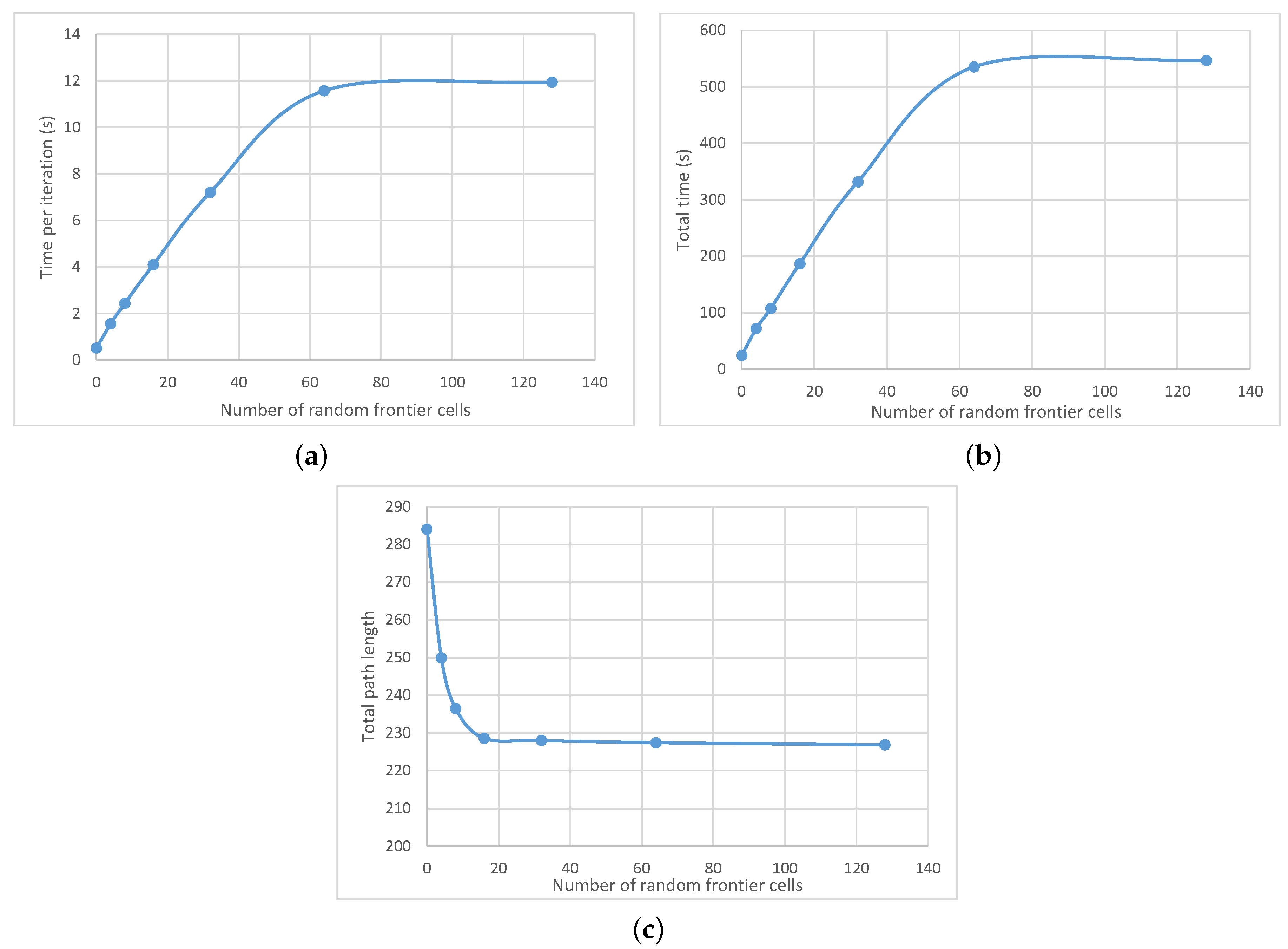
It is evident from Table 5 that the number of random cells does not affect neither the total iteration number nor the maximum tether length in a measurable way. The other parameters are affected significantly, and the effect is visually demonstrated in Figure 5. We can see that both the time per iteration as well as total computation time increase linearly with the number of frontier cells sampled, and saturates at around 70 cells, meaning that, in the testing environment, this was approximately the maximum number of frontier cells throughout the simulation. This means that computational penalty would be directly proportional to the number of cells sampled. Thus, by brute-force sampling all the frontier cells in a large high-resolution environment, these computation times can easily exceed any reasonable boundaries.
Looking at Figure 5c, however, it is clear that such an approach is not necessary. While having no randomness in the algorithm and relying only on the two cells closest to the base and the robot results in a very long total path compared to the rest, the total path length saturates very quickly with the number of random frontier cells, and, at 16 cells, it has already completely leveled off. Looking back at computation times though, at eight random cells, the algorithm is almost twice as fast as the one at 16 cells, while the total path length is not much longer. We considered this a good balance and hence went with for our experiments.
5.1.2. Gazebo Simulations
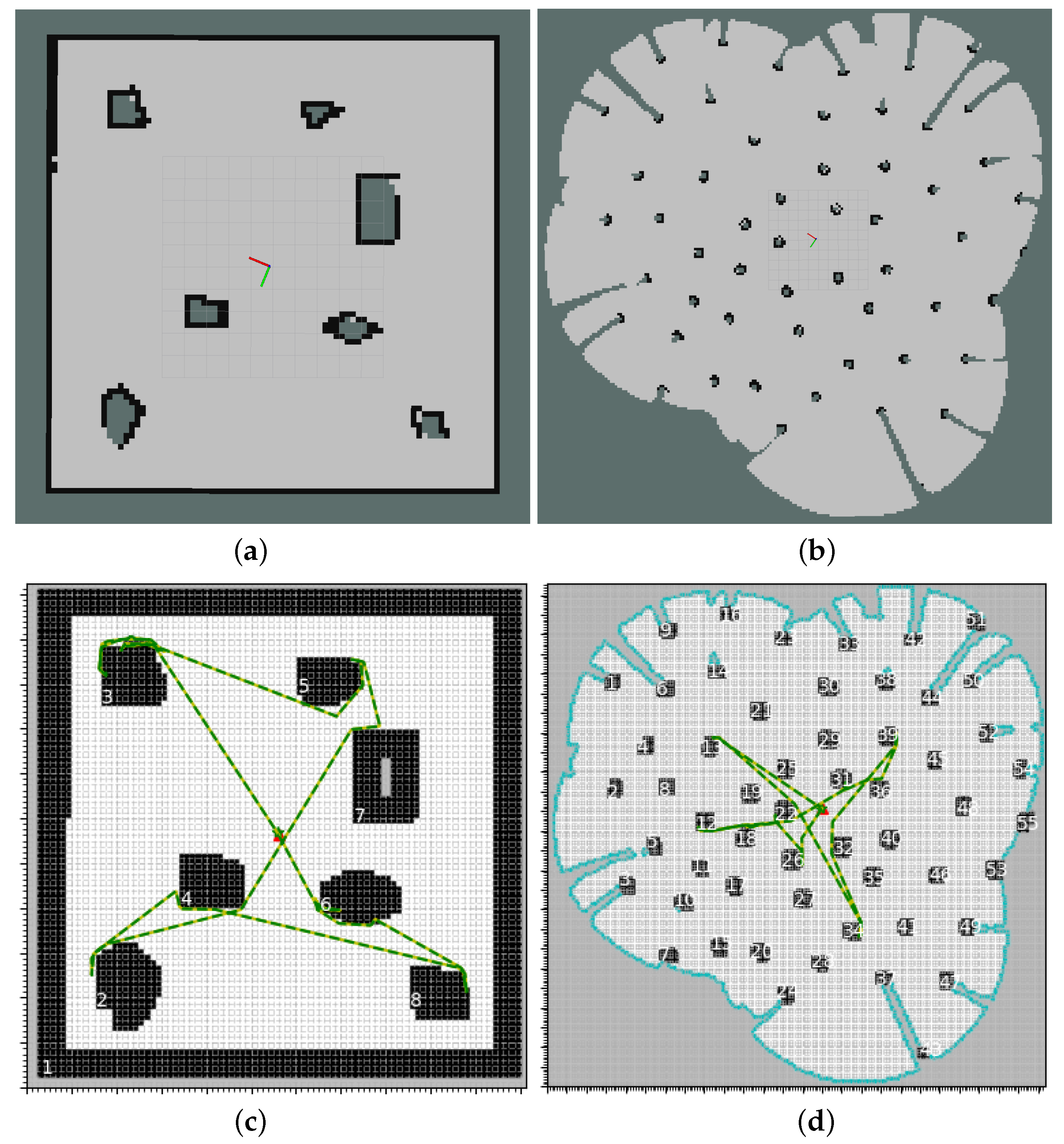
In order to further test the proposed algorithm in a more realistic scenario before fully implementing it on a real robot, we ran two simulations in the Gazebo simulator. Specifically, we simulated a smaller m “room” type environment as well as a bigger unlimited “forest” type environment. Both environments are shown in Figure 6a,b, respectively. A model of the iRobot Create mobile robot equipped with a 360-degree planar LiDAR was used in these simulations. While the “room” environment was a more simplistic test to assess the operation of the algorithm itself, the “forest“ environment was meant to demonstrate how the algorithm behaves in a more dense field where the tether length is the only constraint on the exploration distance. In both cases, maximum tether length was set to 15 m and the length tolerance was set to 4 m, with the latter being just over the theoretical maximum for the ”forest“ environment. This further demonstrates the viability of letting go slightly over while still having tangle-free global paths.
Since the algorithm assumes a point robot in its operation, which was not an issue for the artificial simulations of the previous subsection, to account for the robot dimension in both Gazebo simulations and real-world experiment, the map interpreter in the algorithm creates the robot configuration space by expanding the detected obstacles radially by the radius of the circular robot used. This approach also has a convenient side-effect of expanding the obstacles over what could have been a few extra frontier cells behind an obstacle, saving the robot some unnecessary movement.
Results from Gazebo simulations of both environments can be seen in Figure 7. The “room” environment was fairly straightforward, with the robot completely exploring the environment and returning to the base without tangling the tether, as expected. The “forest” environment is a bit more involved, with a much larger number of obstacles and no external borders. However, as shown in Figure 7d, the robot still managed to explore all the space it could reach with the tether length constraint, while also keeping the tether tangle-free throughout the exploration process. Videos of these simulations can be seen here: https://www.shorturl.at/bcdDW.
5.2. Real World Experiment
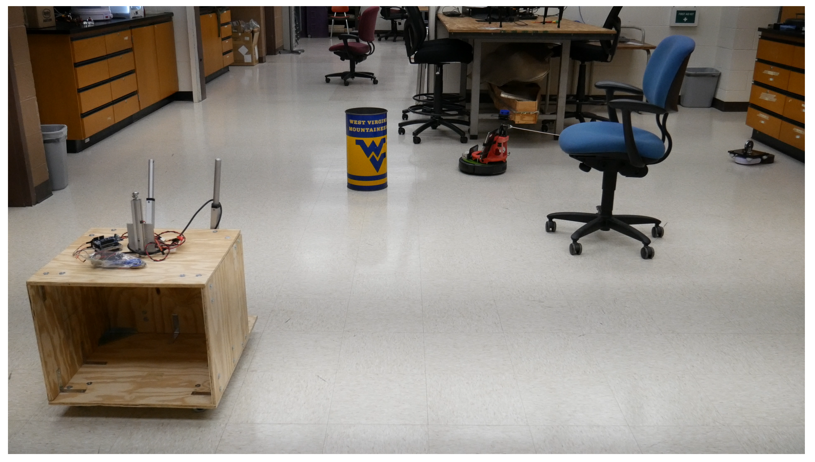
We used a real robot to fully explore our research lab environment with some extra obstacles placed around. The picture of the environment is shown in Figure 8. We have used an iRobot Create 2 equipped with the YDLIDAR X4 360-degree planar LiDAR scanner. A retractile tether spool was anchored to the robot’s base and starting point for the exploration. The tether spool is spring loaded, so the tether is always kept in a taut condition, and the tether itself was attached to a pole on the robot in a way that allowed it to rotate freely, eliminating the possibility of the tether tangling around the robot itself. The robot is controlled with a small laptop computer running Linux Ubuntu 18.04 with an Intel® CoreTM i3 processor clocked at 1.8 GHz.
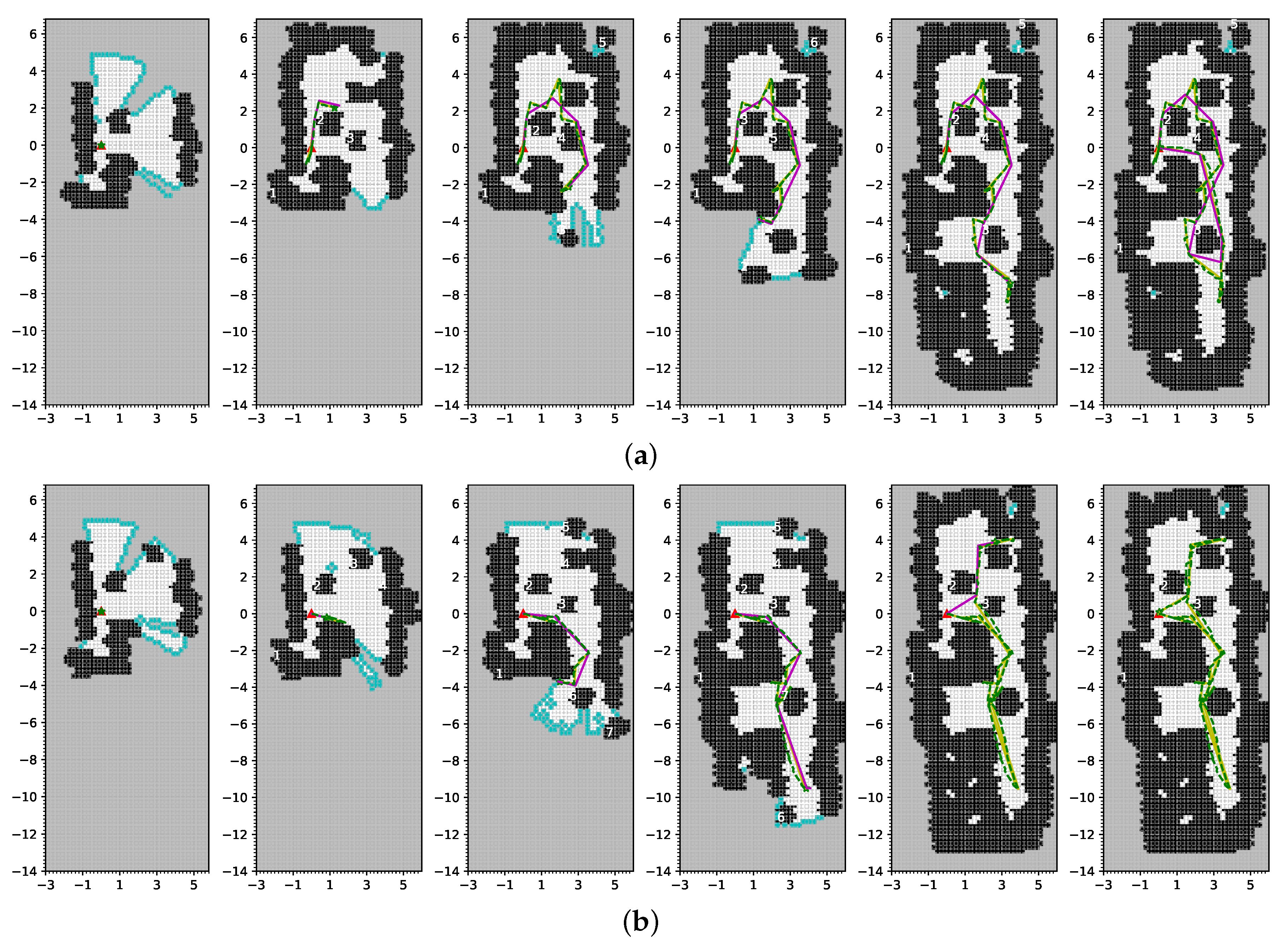
We ran two separate instances of the experiment—one using standard frontier-based exploration, and one using our proposed algorithm. Snapshots of the map building process for these two runs are shown in Figure 9a,b, respectively. In these figures, the robot base is shown as a red triangle and the robot’s position is shown as a green star. Computed paths that the robot was required to take are shown in solid yellow, and the robot’s true paths as reported by the SLAM system are shown in dashed green. The true path and computed path are very close to each other on the figures, making them hard to separate visually, meaning the robot was following the desired path with minimal deviations. Lastly, the tether approximation that was used throughout the exploration is shown in solid purple. As evident from these figures, the standard frontier-based approach that ignored the tether ended up with major tangling, which is visualized by the tether shown in purple being looped around multiple obstacles across the entire testing environment as the robot returned to the base after concluding the exploration. On the other hand, our proposed approach successfully explored the entire environment while keeping the tether in a tangle-free configuration at all times, as the tether is completely retracted by the time the exploration concluded. A video containing similar experiments can be found at https://youtu.be/52bhZoiNjF0.
6. Conclusions
This paper proposes an algorithm for tangle-free exploration of 2D environments with a tethered mobile robot. The algorithm was proven correct given the right choice of parameter , which is used to decide when the robot needs to retract its tether to avoid tangling. Although our proof determines a maximum value for this parameter as a function of the size of the obstacles in the environment, we show experimentally that tangle-free exploration is still possible even with larger errors in this parameter. This is an important characteristic, since we usually do not know the actual size of the obstacles before starting the exploration of an environment. Our results show the effectiveness of our algorithm in both bounded and unbounded spaces, indicating that it can be directly used for exploring any arbitrary environment with a tethered robot.
While we have initially described a generalized algorithm that can use any method both for path planning and for goal selection, our implementation is based on a modified frontier-based exploration approach. Our testing has demonstrated that the total path length in our approach is 30 to 80% longer than the one in an untethered frontier-based exploration method depending on the environment size and obstacle density, and it is also approximately six times shorter than the total path length in a simple backtracking method.
The next logical step in our research is the extension of our algorithm to 3D environments. Even though we have successfully tested the algorithm on simulated drones, we still reduced the drone motion to the plane (see a video here: https://youtu.be/A6A7--rLkfo). While the proposed algorithm itself can work both in 2D and 3D and several techniques can be used for 3D mapping [29,30], defining h-signatures and getting accurate tether configuration data becomes much more complex in 3D. Further research is required in this aspect.
Author Contributions
Conceptualization, D.S. and G.A.S.P.; methodology, D.S.; software, D.S. and G.A.S.P.; validation, D.S.; formal analysis, D.S. and G.A.S.P.; investigation, D.S.; data curation, D.S.; writing—original draft preparation, D.S.; writing—review and editing, D.S. and G.A.S.P.; visualization, D.S. and G.A.S.P.; supervision, G.A.S.P.; project administration, G.A.S.P.; funding acquisition, G.A.S.P. All authors have read and agreed to the published version of the manuscript.
Funding
This research was made possible by the NASA Established Program to Stimulate Competitive Research, Grant #80NSSC19M0054, and the Statler College of West Virginia University.
Conflicts of Interest
The authors declare no conflict of interest.
References
- Barker, L.D.; Jakuba, M.V.; Bowen, A.D.; German, C.R.; Maksym, T.; Mayer, L.; Boetius, A.; Dutrieux, P.; Whitcomb, L.L. Scientific Challenges and Present Capabilities in Underwater Robotic Vehicle Design and Navigation for Oceanographic Exploration Under-Ice. Remote Sens. 2020, 12, 2588. [Google Scholar] [CrossRef]
- Rogers, J.G., III; Sherrill, R.E.; Schang, A.; Meadows, S.L.; Cox, E.P.; Byrne, B.; Baran, D.G.; Curtis, J.W., III; Brink, K.M. Distributed subterranean exploration and mapping with teams of UAVs. In Ground/Air Multisensor Interoperability, Integration, and Networking for Persistent ISR VIII; International Society for Optics and Photonics: Anaheim, CA, USA, 2017; Volume 10190, p. 1019017. [Google Scholar]
- Zhao, J.; Gao, J.; Zhao, F.; Liu, Y. A search-and-rescue robot system for remotely sensing the underground coal mine environment. Sensors 2017, 17, 2426. [Google Scholar] [CrossRef] [PubMed] [Green Version]
- Yamauchi, B.; Schultz, A.; Adams, W. Mobile robot exploration and map-building with continuous localization. In Proceedings of the 1998 IEEE International Conference on Robotics and Automation (Cat. No. 98CH36146), Leuven, Belgium, 20 May 1998; Volume 4, pp. 3715–3720. [Google Scholar]
- Yamauchi, B. A frontier-based approach for autonomous exploration. In Proceedings of the 1997 IEEE International Symposium on Computational Intelligence in Robotics and Automation CIRA’97.’Towards New Computational Principles for Robotics and Automation’, Monterey, CA, USA, 10–11 July 1997; pp. 146–151. [Google Scholar]
- Rekleitis, I.M.; Dudek, G.; Milios, E.E. Graph-based exploration using multiple robots. In Distributed Autonomous Robotic Systems 4; Springer: Berlin/Heidelberg, Germany, 2000; pp. 241–250. [Google Scholar]
- Vallvé, J.; Andrade-Cetto, J. Potential information fields for mobile robot exploration. Robot. Auton. Syst. 2015, 69, 68–79. [Google Scholar] [CrossRef] [Green Version]
- Silva, E.P., Jr.; Engel, P.M.; Trevisan, M.; Idiart, M.A. Exploration method using harmonic functions. Robot. Auton. Syst. 2002, 40, 25–42. [Google Scholar] [CrossRef]
- Bourgault, F.; Makarenko, A.A.; Williams, S.B.; Grocholsky, B.; Durrant-Whyte, H.F. Information based adaptive robotic exploration. In Proceedings of the IEEE/RSJ International Conference on Intelligent Robots and Systems, Lausanne, Switzerland, 30 September–4 October 2002; Volume 1, pp. 540–545. [Google Scholar]
- Elfes, A. Occupancy grids: A stochastic spatial representation for active robot perception. In Proceedings of the Sixth Conference on Uncertainty in AI, Cambridge, MA, USA, 27–29 July 1990; Volume 2929, p. 6. [Google Scholar]
- Mei, Y.; Lu, Y.H.; Lee, C.G.; Hu, Y.C. Energy-efficient mobile robot exploration. In Proceedings of the 2006 IEEE International Conference on Robotics and Automation (ICRA 2006), Orlando, FL, USA, 15–19 May 2006; pp. 505–511. [Google Scholar]
- McGarey, P.; Pomerleau, F.; Barfoot, T.D. System design of a tethered robotic explorer (TReX) for 3D mapping of steep terrain and harsh environments. In Field and Service Robotics; Springer: Berlin/Heidelberg, Germany, 2016; pp. 267–281. [Google Scholar]
- Bowen, A.; German, C.; Jakuba, M.; Kinsey, J.C.; Mayer, L.; Yoerger, D.; Whitcomb, L.L. Lightly tethered unmanned underwater vehicle for under-ice exploration. In Proceedings of the 2012 IEEE Aerospace Conference, Big Sky, MT, USA, 3–10 March 2012; pp. 1–12. [Google Scholar]
- Iqbal, J.; Heikkila, S.; Halme, A. Tether tracking and control of ROSA robotic rover. In Proceedings of the 2008 10th International Conference on Control, Automation, Robotics and Vision, Hanoi, Vietnam, 17–20 December 2008; pp. 689–693. [Google Scholar]
- McGarey, P.M. Towards Autonomy and Mobility for a Tethered Robot Exploring Extremely Steep Terrain. Ph.D. Thesis, University of Toronto, Toronto, ON, Canada, 2017. [Google Scholar]
- Igarashi, T.; Stilman, M. Homotopic path planning on manifolds for cabled mobile robots. In Algorithmic Foundations of Robotics IX; Springer: Berlin/Heidelberg, Germany, 2010; pp. 1–18. [Google Scholar]
- Kim, S.; Bhattacharya, S.; Kumar, V. Path planning for a tethered mobile robot. In Proceedings of the 2014 IEEE International Conference on Robotics and Automation (ICRA), Hong Kong, China, 31 May–7 June 2014; pp. 1132–1139. [Google Scholar]
- LaValle, S.M. Rapidly-Exploring Random Trees: A New Tool for Path Planning; Technical Report; Computer Science Dept., Iowa State University: Ames, IA, USA, 1998. [Google Scholar]
- Hernandez, E.; Carreras, M.; Ridao, P. A comparison of homotopic path planning algorithms for robotic applications. Robot. Auton. Syst. 2015, 64, 44–58. [Google Scholar] [CrossRef]
- Yi, D.; Goodrich, M.A.; Seppi, K.D. Homotopy-aware RRT*: Toward human-robot topological path-planning. In Proceedings of the 2016 11th ACM/IEEE International Conference on Human-Robot Interaction (HRI), Christchurch, New Zealand, 7–10 March 2016; pp. 279–286. [Google Scholar]
- Sakcak, B.; Bascetta, L.; Ferretti, G. Homotopy aware kinodynamic planning using RRT-based planners. In Proceedings of the 2019 18th European Control Conference (ECC), Naples, Italy, 25–28 June 2019; pp. 1568–1573. [Google Scholar]
- Kim, S.; Likhachev, M. Path planning for a tethered robot using Multi-Heuristic A* with topology-based heuristics. In Proceedings of the 2015 IEEE/RSJ International Conference on Intelligent Robots and Systems (IROS), Hamburg, Germany, 28 September–2 October 2015; pp. 4656–4663. [Google Scholar]
- Shapovalov, D.; Pereira, G.A.S. Exploration of unknown environments with a tethered mobile robot. In Proceedings of the 2020 IEEE/RSJ International Conference on Intelligent Robots and Systems (IROS), Las Vegas, NV, USA, 25–29 October 2020; pp. 6826–6831. [Google Scholar]
- Shnaps, I.; Rimon, E. Online coverage by a tethered autonomous mobile robot in planar unknown environments. IEEE Trans. Robot. 2014, 30, 966–974. [Google Scholar] [CrossRef]
- Sharma, G.; Poudel, P.; Dutta, A.; Zeinali, V.; Khoei, T.T.; Kim, J.H. A 2-Approximation Algorithm for the Online Tethered Coverage Problem. Proceedings of Robotics: Science and Systems (RSS), Freiburg im Breisgau, Germany, 22–26 June 2019. [Google Scholar]
- Choset, H.M.; Hutchinson, S.; Lynch, K.M.; Kantor, G.; Burgard, W.; Kavraki, L.E.; Thrun, S.; Arkin, R.C. Principles of Robot Motion: Theory, Algorithms, and Implementation; MIT Press: Cambridge, MA, USA, 2005. [Google Scholar]
- Quigley, M.; Gerkey, B.; Conley, K.; Faust, J.; Foote, T.; Leibs, J.; Berger, E.; Wheeler, R.; Ng, A. ROS: An open-source Robot Operating System. In Proceedings of the IEEE IInternational Conference on Robotics and Automation (ICRA) Workshop on Open Source Robotics, Kobe, Japan, 12–17 May 2009. [Google Scholar]
- Koenig, N.; Howard, A. Design and Use Paradigms for Gazebo, An Open-Source Multi-Robot Simulator. In Proceedings of the IEEE/RSJ International Conference on Intelligent Robots and Systems (IROS), Sendai, Japan, 28 September–2 October 2004; pp. 2149–2154. [Google Scholar]
- Zhu, Q.; Wang, Z.; Hu, H.; Xie, L.; Ge, X.; Zhang, Y. Leveraging photogrammetric mesh models for aerial-ground feature point matching toward integrated 3D reconstruction. ISPRS J. Photogramm. Remote Sens. 2020, 166, 26–40. [Google Scholar] [CrossRef]
- Cui, H.; Shi, T.; Zhang, J.; Xu, P.; Meng, Y.; Shen, S. View-graph Construction Framework for Robust and Efficient Structure-from-Motion. Pattern Recognit. 2020, 107712. [Google Scholar] [CrossRef]
Figure 1.
Visual representation of our proposed approach. The robot at the position with a tether connecting it to the base at compares the shortest path to the goal from the base () with the one from its current position (), and takes the path to return the tether to its shortest configuration and avoid further tangling.

Figure 2.
(a) three example paths from to . Paths and are homotopic to each other and therefore lie in the same homotopy class, while in in a different homotopy class; (b) three example paths from to . h-signature of is which reduces to , h-signature of is 0, and h-signature of is .
Figure 2.
(a) three example paths from to . Paths and are homotopic to each other and therefore lie in the same homotopy class, while in in a different homotopy class; (b) three example paths from to . h-signature of is which reduces to , h-signature of is 0, and h-signature of is .

Figure 3.
Flowchart representing the proposed exploration algorithm.

Figure 4.
Typical randomized environments used in simulations. Shown are typical configurations for low-density environment (a), high-density environment (b) and large environment (c), as well as example paths taken to explore them, shown in (d–f), respectively.
Figure 4.
Typical randomized environments used in simulations. Shown are typical configurations for low-density environment (a), high-density environment (b) and large environment (c), as well as example paths taken to explore them, shown in (d–f), respectively.

Figure 5.
Illustration of the data from Table 5. The effect of the number of random frontier cells on time per iteration (a), total computation time (b) and total path length (c).
Figure 5.
Illustration of the data from Table 5. The effect of the number of random frontier cells on time per iteration (a), total computation time (b) and total path length (c).

Figure 6.
Environments used in Gazebo simulations. “Room” type environment is shown in (a), and “forest” type environment is shown in (b).
Figure 6.
Environments used in Gazebo simulations. “Room” type environment is shown in (a), and “forest” type environment is shown in (b).

Figure 7.
Results from Gazebo simulations. Maps generated my gmapping for room and forest environments are shown in (a,b) respectively, and internal algorithm maps for them with expanded obstacles and total paths taken being shown in (c,d) respectively.
Figure 7.
Results from Gazebo simulations. Maps generated my gmapping for room and forest environments are shown in (a,b) respectively, and internal algorithm maps for them with expanded obstacles and total paths taken being shown in (c,d) respectively.

Figure 8.
Lab environment used for the experiment.

Figure 9.
Snapshots of map building during during the real world experiment. Standard frontier-based exploration is shown in (a), and our proposed approach is shown in (b). The tether approximation during the exploration is shown in purple.
Figure 9.
Snapshots of map building during during the real world experiment. Standard frontier-based exploration is shown in (a), and our proposed approach is shown in (b). The tether approximation during the exploration is shown in purple.


Table 1.
Simulation data for low density environment. map, resolution, tether length 40, 15–20 obstacles of radius up to 2. Tether base is at [1, 1], and the field of view is set to 4.
Table 1.
Simulation data for low density environment. map, resolution, tether length 40, 15–20 obstacles of radius up to 2. Tether base is at [1, 1], and the field of view is set to 4.
| Tolerance | Tangle (%) | Time per Iteration (s) | Total Time (s) | Total Iterations | Max Tether Length | Total Path Length |
|---|---|---|---|---|---|---|
| Backtrack | 0 | 0.063 ± 0.005 | 2.611 ± 0.323 | 41.5 ± 2.5 | 24.129 ± 0.912 | 1120.101 ± 78.904 |
| 0 | 0 | 1.000 ± 0.184 | 37.727 ± 7.629 | 37.0 ± 2.6 | 27.742 ± 5.800 | 187.544 ± 39.293 |
| 2R | 0 | 0.979 ± 0.123 | 36.335 ± 5.545 | 37.0 ± 2.8 | 29.937 ± 4.696 | 169.000 ± 29.433 |
| 4R | 0 | 1.051 ± 0.153 | 39.174 ± 6.963 | 37.2 ± 3.0 | 32.431 ± 4.264 | 165.251 ± 19.336 |
| 8R | 14 | 1.120 ± 0.143 | 42.239 ± 6.951 | 37.6 ± 2.2 | 36.147 ± 3.192 | 170.364 ± 23.007 |
| 16R | 28 | 1.264 ± 0.220 | 48.757 ± 9.515 | 38.5 ± 2.1 | 39.014 ± 0.940 | 173.233 ± 21.557 |
| ∞ | 44 | 1.339 ± 0.366 | 53.098 ± 12.331 | 39.2 ± 2.8 | 39.476 ± 0.685 | 171.970 ± 26.533 |
| ∞ () | 88 | 0.270 ± 0.089 | 10.554 ± 3.745 | 38.8 ± 2.8 | 78.129 ± 18.817 | 126.714 ± 14.293 |
Table 2.
Simulation data for high density environment. map, resolution, tether length 40, 50–60 obstacles of radius up to . Tether base is at [1, 1], and the field of view is set to 4.
Table 2.
Simulation data for high density environment. map, resolution, tether length 40, 50–60 obstacles of radius up to . Tether base is at [1, 1], and the field of view is set to 4.
| Tolerance | Tangle (%) | Time per Iteration (s) | Total Time (s) | Total Iterations | Max Tether Length | Total Path Length |
|---|---|---|---|---|---|---|
| Backtrack | 0 | 0.076 ± 0.051 | 3.558 ± 0.383 | 46.5 ± 3.0 | 24.673 ± 0.754 | 1269.056 ± 92.467 |
| 0 | 0 | 2.256 ± 0.470 | 100.280 ± 24.641 | 44.2 ± 3.2 | 26.479 ± 3.282 | 292.230 ± 42.446 |
| 2R | 0 | 2.440 ± 0.453 | 107.576 ± 22.351 | 43.9 ± 2.3 | 26.721 ± 1.481 | 236.458 ± 25.719 |
| 4R | 6 | 2.625 ± 0.733 | 120.867 ± 39.459 | 45.6 ± 3.1 | 30.550 ± 2.292 | 225.613 ± 27.852 |
| 8R | 12 | 2.974 ± 0.607 | 139.431 ± 31.309 | 46.7 ± 3.1 | 35.543 ± 2.435 | 223.947 ± 21.973 |
| 16R | 32 | 3.174 ± 0.979 | 154.725 ± 51.098 | 46.9 ± 3.0 | 39.178 ± 0.689 | 225.708 ± 19.908 |
| ∞ | 54 | 3.241 ± 1.054 | 153.764 ± 53.731 | 47.1 ± 3.0 | 39.200 ± 0.722 | 228.256 ± 23.976 |
| ∞ () | 98 | 1.484 ± 0.554 | 70.894 ± 29.271 | 47.2 ± 3.3 | 102.364 ± 13.341 | 145.629 ± 13.175 |
Table 3.
Simulation data for large environment. map, resolution, tether length 40, 40–50 obstacles of radius up to 2. Tether base is at [20, 20], and the field of view is set to 10.
Table 3.
Simulation data for large environment. map, resolution, tether length 40, 40–50 obstacles of radius up to 2. Tether base is at [20, 20], and the field of view is set to 10.
| Tolerance | Tangle (%) | Time per Iteration (s) | Total Time (s) | Total Iterations | Max Tether Length | Total Path Length |
|---|---|---|---|---|---|---|
| Backtrack | 0 | 0.526 ± 0.031 | 34.285 ± 4.214 | 65.0 ± 5.1 | 26.661 ± 0.980 | 2032.611 ± 173.774 |
| 0 | 0 | 5.564 ± 0.912 | 357.424 ± 74.419 | 63.9 ± 5.1 | 27.401 ± 1.335 | 667.252 ± 71.126 |
| 2R | 0 | 5.573 ± 0.697 | 360.587 ± 59.524 | 64.5 ± 4.3 | 28.351 ± 1.771 | 533.391 ± 53.077 |
| 4R | 2 | 5.942 ± 1.056 | 393.569 ± 86.561 | 65.9 ± 4.9 | 30.658 ± 1.449 | 516.228 ± 71.644 |
| 8R | 20 | 6.177 ± 0.924 | 417.102 ± 75.505 | 67.3 ± 4.0 | 35.225 ± 1.967 | 481.901 ± 42.814 |
| 16R | 32 | 6.466 ± 0.862 | 441.738 ± 64.365 | 68.3 ± 4.4 | 39.385 ± 0.522 | 489.221 ± 38.029 |
| ∞ | 48 | 6.618 ± 0.869 | 454.108 ± 68.735 | 68.5 ± 3.4 | 39.534 ± 0.384 | 498.749 ± 43.545 |
| ∞ () | 96 | 5.091 ± 1.404 | 375.764 ± 108.251 | 73.6 ± 3.9 | 218.189 ± 23.007 | 285.281 ± 19.157 |
Table 4.
Results using true distance to frontiers at .
| Environment Type | Tangle (%) | Time per Iteration (s) | Total Time (s) | Total Iterations | Max Tether Length | Total Path Length |
|---|---|---|---|---|---|---|
| Low density | 0 | 4.095 ± 0.751 | 157.243 ± 33.027 | 38.3 ± 2.8 | 30.322 ± 4.843 | 171.551 ± 20.323 |
| High density | 0 | 6.937 ± 1.279 | 315.000 ± 67.851 | 45.2 ± 2.9 | 27.432 ± 2.320 | 239.675 ± 26.978 |
Table 5.
Results using varying numbers of random frontier cells at in a high-density environment.
| Cells Sampled | Time per Iteration (s) | Total Time (s) | Total Iterations | Max Tether Length | Total Path Length |
|---|---|---|---|---|---|
| 0 | 0.515 ± 0.128 | 24.174 ± 7.017 | 46.6 ± 2.9 | 27.295 ± 2.540 | 284.044 ± 32.336 |
| 4 | 1.562 ± 0.534 | 71.740 ± 25.452 | 45.7 ± 2.8 | 27.067 ± 1.797 | 249.882 ± 30.136 |
| 8 | 2.440 ± 0.453 | 107.576 ± 22.351 | 43.9 ± 2.3 | 26.721 ± 1.481 | 236.458 ± 25.719 |
| 16 | 4.099 ± 0.841 | 186.638 ± 43.164 | 45.4 ± 2.5 | 28.081 ± 2.797 | 228.557 ± 26.656 |
| 32 | 7.206 ± 1.592 | 331.824 ± 84.986 | 45.8 ± 2.9 | 27.682 ± 2.088 | 227.961 ± 24.718 |
| 64 | 11.576 ± 2.896 | 535.286 ± 147.438 | 46.0 ± 2.7 | 28.042 ± 2.215 | 227.405 ± 28.321 |
| 128 | 11.937 ± 3.171 | 546.617 ± 159.215 | 45.5 ± 3.1 | 27.969 ± 2.637 | 226.805 ± 27.268 |
Publisher’s Note: MDPI stays neutral with regard to jurisdictional claims in published maps and institutional affiliations. |
© 2020 by the authors. Licensee MDPI, Basel, Switzerland. This article is an open access article distributed under the terms and conditions of the Creative Commons Attribution (CC BY) license (http://creativecommons.org/licenses/by/4.0/).
Share and Cite
MDPI and ACS Style
Shapovalov, D.; Pereira, G.A.S. Tangle-Free Exploration with a Tethered Mobile Robot. Remote Sens. 2020, 12, 3858. https://0-doi-org.brum.beds.ac.uk/10.3390/rs12233858
AMA Style
Shapovalov D, Pereira GAS. Tangle-Free Exploration with a Tethered Mobile Robot. Remote Sensing. 2020; 12(23):3858. https://0-doi-org.brum.beds.ac.uk/10.3390/rs12233858
Chicago/Turabian StyleShapovalov, Danylo, and Guilherme A. S. Pereira. 2020. "Tangle-Free Exploration with a Tethered Mobile Robot" Remote Sensing 12, no. 23: 3858. https://0-doi-org.brum.beds.ac.uk/10.3390/rs12233858
Note that from the first issue of 2016, this journal uses article numbers instead of page numbers. See further details here.