Article

Early Detection of Ganoderma boninense in Oil Palm Seedlings Using Support Vector Machines

by
Aiman Nabilah Noor Azmi
1,
Siti Khairunniza Bejo
1,2,3,*,
Mahirah Jahari
1,
Farrah Melissa Muharam
4,
Ian Yule
5 and
Nur Azuan Husin
1
1
Department of Biological and Agricultural Engineering, Faculty of Engineering, Universiti Putra Malaysia, Serdang 43400, Malaysia
2
Smart Farming Technology Research Centre, Faculty of Engineering, Universiti Putra Malaysia, Serdang 43400, Malaysia
3
Institute of Plantation Studies, Universiti Putra Malaysia, Serdang 43400, Malaysia
4
Department of Agriculture Technology, Faculty of Agriculture, Universiti Putra Malaysia, Serdang 43400, Malaysia
5
Institute of Agriculture and Environment, Massey University, Private Bag, Palmerston North 11222, New Zealand
*
Author to whom correspondence should be addressed.
Remote Sens. 2020, 12(23), 3920; https://0-doi-org.brum.beds.ac.uk/10.3390/rs12233920
Submission received: 5 October 2020 / Revised: 21 November 2020 / Accepted: 23 November 2020 / Published: 29 November 2020
(This article belongs to the Special Issue Remote Sensing for Precision Agriculture)

Abstract

:
Ganodermaboninense (G. boninense) is a fungus that causes one of the most destructive diseases in oil palm plantations in Southeast Asia called basal stem rot (BSR), resulting in annual losses of up to USD 500 million. The G. boninense infects both mature trees and seedlings. The current practice of detection still depends on manual inspection by a human expert every two weeks. This study aimed to detect early G. boninense infections using visible-near infrared (VIS-NIR) hyperspectral images where there are no BSR symptoms present. Twenty-eight samples of oil palm seedlings at five months old were used whereby 15 of them were inoculated with the G. boninense pathogen. Five months later, spectral reflectance oil palm leaflets taken from fronds 1 (F1) and 2 (F2) were obtained from the VIS-NIR hyperspectral images. The significant bands were identified based on the high separation between uninoculated (U) and inoculated (I) seedlings. The results indicate that the differences were evidently seen in the NIR spectrum. The bands were later used as input parameters for the development of Support Vector Machine (SVM) classification models, and these bands were optimized according to the classification accuracy achieved by the classifiers. It was observed that the U and I seedlings were excellently classified with 100% accuracy using 35 bands and 18 bands of F1. However, the combination of F1 and F2 (F12) gave better accuracy than F2 and almost similar to F1 for specific classifiers. This finding will provide an advantage when using aerial images where there is no need to separate F1 and F2 during the data pre-processing stage.

Graphical Abstract

1. Introduction

The production of oil palm in Southeast Asia has been affected by a never-ending case of basal stem rot (BSR) disease. Malaysia has reported annual losses of up to RM 1.5 billion due to this disease, which has made it the most economically devastating disease in the agricultural field. Not only the mature trees, but the oil palm seedlings are also susceptible to the infection whereby the symptoms appear earlier and more severe [1]. BSR affects a plantation by reducing the number of standing trees as well as the weight of fresh fruit bunches (FFB) [2]. According to Subagio and Foster [3], FFB yield decreases by an average of 0.16 tons per hectare for every dead palm or equivalent to 35% when half of the planted trees have died. Based on the BSR incident rate, the total area affected in 2020 was estimated to be 443,440 hectares, equivalent to 65.6 million oil palms, which is worrying if preventative measures are not implemented [4]. BSR could cause 80% of the affected trees to die [5]. However, the trees with an infection of less than 20% can still be treated [6].
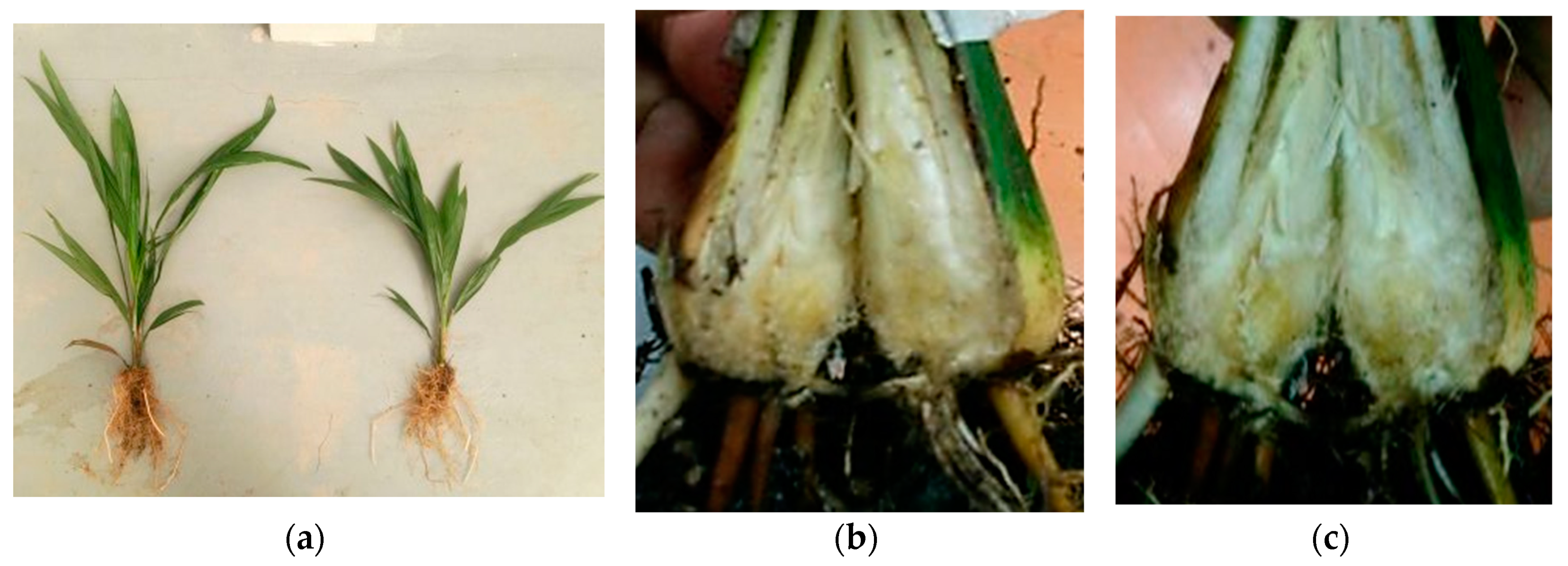
G. boninense infection affects the xylem, which causes a major problem in water and nutrient distribution, making the symptoms appear similar to water stress and nutrient deficiency. The earliest visual symptom in seedlings can be seen in the presence of a fruiting body at the bole and followed by partial yellowing of older leaves or mottling of basal fronds to form necrosis, indicating that over 50% of the stem base has been internally damaged [7]. However, the fruiting body may present or may not before or after the development of foliar symptoms [5,8], making visual identification hard, confusing, and often overlooked. In a severe infection, there is no development of new leaves, no increase in height or girth that will consequently lead to growth inhibition. These are all attributed to the inability of the plant to perform normal photosynthesis due to low chlorophyll content and water deficiency [9]. Despite the visual symptoms, G. boninense infection can also be detected in the roots and longitudinal sectioning of the infected bole. The longitudinal section usually shows brown discoloration with white mycelium protruding through the root epidermis, indicating upward infection progress within the seedling. Nevertheless, detection through the bole and roots is impractical for large-scale planting areas as the process is labor intensive and causes injury that could lead to tree destruction.
Early detection, timely prevention, and control are indispensable to counter this disease. Nowadays, G. boninense infection can be detected by various methods. For example, (i) a colorimetric method using ethylenediaminetetraacetic acid (EDTA) [10], (ii) Ganoderma-selective medium (GSM) [11], (iii) polyclonal antibodies (PAbs) [12,13], (iv) enzyme-linked immunosorbent assay (ELISA) [14,15], (v) polymerase chain reaction (PCR) [16,17], (vi) an electronic nose (e-nose) device [18,19], (vii) microfocus X-ray fluorescence (μXRF) [6] (viii) tomography images [20], and (ix) a terrestrial laser scanner (TLS) device [21,22,23]. Nonetheless, these methods are time consuming, impractical for large-scale plantations, and some comprise stem collection and laboratory procedures, which are expensive, tedious, require trained specialists, and appropriate laboratory facilities.
Hyperspectral remote sensing is widely used due to its ability to capture light reflected from plants in narrow and contiguous wavelengths. Every pixel in the image contains a complete spectral reflectance that is well associated with varying degrees and types of stresses [24,25,26,27,28,29,30]. Healthy plants usually exhibit lower visible reflectance and higher near infrared (NIR) reflectance, whereas unhealthy plants show different spectral patterns depending on the physiology and morphology of the leaves. Advanced data mining analyses can be used to assess vegetation stress; for example, principal component analysis (PCA) [31,32], machine learning classification [29,30,33,34], spectral derivative analysis [35,36,37] and vegetation indices [38,39]. Rumpf et al. [40] combined vegetation indices and SVM to determine healthy and diseased sugar beet leaves caused by Cercospora beticola. The result showed up to 97% classification accuracy. Nagasubramanian et al. [41] proved the strength of hyperspectral reflectance over red, green and blue (RGB) data by detecting charcoal rot disease in soybean stem using SVM and obtained 97% and 78% accuracy, respectively.
Nevertheless, the application of hyperspectral imaging to detect BSR in oil palm seedlings has not yet been explored. Instead, it has been applied in several studies of BSR detection in mature oil palm by utilizing an Airborne Imaging Spectrometer for Applications (AISA) imaging system [42,43,44,45,46]. These studies were majorly focused on the development of optimal vegetation indices to differentiate between different levels of severity of the BSR disease. However, only a study conducted by Shafri et al. [44] produced a satisfactorily result with 86% overall accuracy. Alternatively, for oil palm seedlings, other researchers utilized spectroscopy devices to acquire spectral information such as the study performed by Shafri and Anuar [47], who identified significant bands to distinguish between different severity levels of G. boninense infection. However, there was poor discrimination between healthy and mildly infected seedlings due to overlapping reflectance spectra between these classes. Similarly, Shafri et al. [48] also encountered challenges to differentiate between healthy and mildly infected seedlings (inoculated at four months old) after six months of inoculation. Their study used significant bands of first derivative spectra to develop a Maximum Likelihood classification model. The accuracy produced by the model was 82% with a kappa coefficient of 0.73.
Table 1 gives a summary of methods and specific bands used to detect BSR disease in oil palm seedlings and mature trees. As observed, previous studies have been able to present good discrimination accuracy between healthy and infected trees/seedlings with the highest accuracy of 82% and 97% at nursery and plantation level, respectively. Only six out of 20 research studies focused on BSR detection at nursery level using spectroscopy devices with the best method found to be conventional classification, i.e., Maximum Likelihood, and none of the methods used hyperspectral imaging and machine learning techniques. Although the spectroscopy device is capable of detecting early infection of BSR in oil palm seedlings, it has a limitation where the device can only take one reading per time for a small sample point, thus requiring a longer duration of data collection. In contrast, a hyperspectral camera can reduce the time taken for data collection due to its ability to cover large areas in a single imaging session.
The use of machine learning techniques, especially Support Vector Machines (SVMs), has been shown to be beneficial in agriculture applications [30,49,50,51,52,53] and is worth being explored, especially for early detection of BSR such as in studies conducted by Santoso et al. [54], Santoso et al. [55] and Khaled et al. [
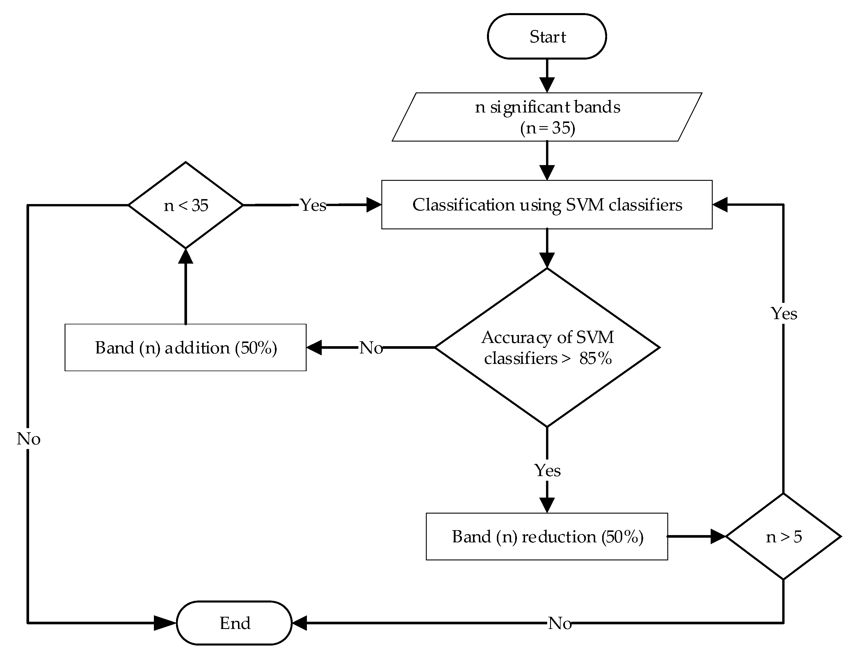
56]. SVM offers robust analysis and better prediction due to the optimal hyperplane marginal gap between classes. It has been used for classification, regression, and clustering in agricultural studies. The main advantage of SVM is the implementation of the kernel method, which enables higher dimensional separation of non-linear data and improves the computational power of linear learning machines. Kernel functions that are widely used are linear, Gaussian radial basis function (RBF), and polynomial. In addition, this study was carried out to determine the capability of various SVM classifiers to achieve a high degree of accuracy in classifying the different number of bands, features, and frond number for early detection of G. boninense.

2. Materials and Methods

2.1. Study Area

The study was conducted at the Transgenic Greenhouse, Universiti Putra Malaysia (UPM), Serdang, Malaysia (2°59′33.10″ N, 101°43′19.16″ E), from 24 January 2019 to 24 June 2019. The greenhouse has dimensions of 12 m length x 6 m width x 4 m height and is made up of polycarbonate panels to protect against harmful UV light and is equipped with air conditioners, humidifiers, thermal screens, and a humidity/temperature sensor. The temperature inside the greenhouse was set at 27 °C following the work of Kamil and Omar [69].

2.2. Artificial Inoculation of Samples

A total of 28 oil palm seedlings (commercial standard crosses of Dura × Pisifera, D × P) were obtained from Sime Darby Plantation, Banting, Malaysia, at the age of four months old. The seedlings were permitted to acclimatize under greenhouse conditions for one month before transplanting.
At five months old, 15 of the seedlings were transplanted into 24 cm × 21 cm × 33 cm polybags comprising 30% of a mixture of 90% topsoil and 10% sand. A rubberwood block (RWB, 6 cm × 6 cm × 6 cm) colonized with G. boninense pathogen was placed at the center of a polybag. The roots of the seedlings were positioned on top to have direct contact with the RWB and covered with soil until the bole level. This method is called a sitting technique as described in Naidu et al. [70]. Thirteen seedlings were planted with uninoculated RWB acting as the control treatment (U). All the seedlings were arranged according to the standard triangular arrangement of an oil palm nursery with equal and sufficient water and fertilizer application. Two months after artificial inoculation, two of the inoculated (I) seedlings were sent to the Bacteriology Laboratory, Faculty of Agriculture, UPM, Serdang, Malaysia, for a polymerase chain reaction (PCR) test to confirm the G. boninense infection.

2.3. Data Collection

The process of image acquisition was conducted five months after transplanting. The camera used in this study was a FireflEYE S185 (Cubert GmbH, Ulm, Germany) snapshot camera with wavelengths ranging from 450 to 950 nm (125 bands) that covers the visible (blue, green, and red) and NIR regions with a sampling interval of 4 nm. The camera was mounted horizontally on a custom tripod and was positioned 2.6 m from the ground level (Figure 1).
The camera was calibrated with white and dark references before each image acquisition to reduce the effect of illumination and detector sensitivity. Therefore, the time for integration was approximately the same. The dark calibration was performed by closing the lens of the camera, while the white calibration was performed by placing the provided white rectangular board (99% light reflection) flat and close to the lens. Each collected spectrum was calibrated as:
R e f l e c t a n c e =   ( I m a g e D a r k ) ( W h i t e D a r k )
The white and dark calibrations were checked before the actual image acquisition to ensure good quality of the output images. One seedling was imaged at one time against a black background board. The images were taken on a sunny, clear day from 11:00 a.m. to 2:00 p.m. local time to obtain a natural illumination. The system was controlled by Cube-Pilot software provided by the manufacturer.

2.4. Data Pre-Processing

Figure 2 shows the top view image of frond 1 (F1) and frond 2 (F2). In order to minimize variations in spectral reflectance due to the effects of frond inclination [71], only the spectral reflectance of the first four leaflets of F1 and F2 were extracted manually and randomly. The usage of F1 and F2 followed the work of Shafri et al. [48] and Izzuddin et al. [59] due to the morphological arrangement of the fronds. Therefore, an average of 20 sample points were obtained from each frond, resulting in a total number of 558 and 564 sample points for F1 and F2, respectively. The outliers of the data were identified using the box plot method. Box plot analyzed the data statistically in a graphical manner with five measured parameters representing the distribution, i.e., lower quartile, upper quartile, lower fence, upper fence, and interquartile range. These quartile ranges were advantageous due to their reduced sensitivity towards outliers [72,73].

2.5. Data Analysis

In this study, the detection of G. boninense infection was determined by analyzing specific spectral signatures at different treatments (U and I) as well as at different frond numbers. Bands were selected based on the first 35 bands (30% of the total bands) that gave high separation values between U and I. These bands were also subject to a t-test statistical analysis using SPSS statistical software (IBM SPSS Statistics 25, IBM, New York, NY, USA) with a value of p ≤ 0.05. Then, the coefficient of variation (CV) of the sample points for all significant bands was calculated to identify the dispersion of the data. The CV was calculated as:
C V = s x ¯ × 100 %
where s   is the standard deviation of the samples, and x ¯ is the mean of the samples.
Later, the identified significant bands were used as input parameters to develop SVM classification models using the machine learning toolbox of MATLAB (2019b, The MathWorks Inc., Natick, MA, USA). In order to evaluate the performance of the developed model, a five-fold cross-validation technique was applied where the data was randomly divided into five equal-sized subsamples. Each subsample was used to test the constructed model using the remaining four trained subsamples. This process was repeated five times, with each subsample becomes a testing set once to improve the effectiveness of the model. The completed models were subsequently exported and assessed using the prediction dataset.
In this study SVM classification models with different kernel functions, i.e., linear, Gaussian RBF, and polynomial, were trained. The linear kernel was fit for linearly separable data, which may be expressed as:
k ( x i , x j ) = x i T x j
where k is the kernel function, ( x i , x j ) are a-dimensional input and x i T x j is a map from the a-dimension to the b-dimension.
Where the data are not linearly separable, an appropriate kernel function may be used to enhance SVM classification. The kernel method allows SVM to identify a hyperplane in the kernel space, hence making non-linear separation feasible within the feature space. An example of non-linear kernels is the Gaussian Radial Basis Function (RBF), which can be represented as:
k ( x i , x j ) = exp ( x i x j 2 2 σ 2 ) = exp ( γ x i x j 2 ) ,
where x i x j 2 is known as the squared Euclidean distance between two feature vectors, and σ is defined as the kernel width. A small kernel width tends to reflect dissimilar patterns and causes overfitting, whereas large kernel width results in very similar patterns and causes underfitting. The optimal kernel width is chosen based on a tradeoff between underfitting and overfitting loss. Furthermore, the σ also has a similar definition as the with kernel scale (γ) where =   1 2 σ 2 . In this study, the value of γ was adjusted to different values according to the following assumptions:
γ f G = n / 4 ,   for   fine   Gaussian , γ m G = n ,   for   medium   Gaussian , γ c G = 4 n ,   for   coarse   Gaussian ,
where n is the number of features.
Another kernel function that was used was the polynomial that can be expressed as:
k ( x i , x j ) = ( 1 + x i T x j ) p ,
where p is the order of the polynomial kernel. The degree of the polynomial kernel is able to influence the tolerance of the classifier resulting in a flexible decision boundary of a higher degree polynomial than the lower value.
After the classification models were constructed, an optimization process was carried out to find the optimal number of bands that could give suitable classification accuracy. Exploration runs were applied where the initial number of significant bands was optimized, as shown in Figure 3. Thirty-five significant bands that were confirmed to be statistically significant were used as inputs of the SVM classifiers. If the classification accuracy obtained by all SVM classifiers was greater than 85%, the current number of significant bands was reduced by 50%. Otherwise, if the condition was not satisfied, the current number of significant bands was increased by 50%. The classification models of the reflectance spectra were developed separately for F1, F2, and the combination of F1 and F2 (F12) using the respective significant bands.

3. Results

3.1. Status of the Inoculated Sample

Figure 4 shows the condition of the oil palm seedlings that were sent to the Bacteriology Laboratory, Faculty of Agriculture, UPM for PCR test to confirm G. boninense infection. Both samples tested positive for G. boninense infection, although the seedlings displayed no apparent symptoms associated with BSR disease such as fungal mass and yellowing of older leaves. However, longitudinal sectioning of the bole showed brown discoloration indicating the presence of the G. boninense infection. Furthermore, Figure 5 shows the condition of I seedling after 20 weeks of artificial inoculation. The seedling also did not show any visible symptoms related to G. boninense infection, as stated in Izzati et al. [74]; Kok et al. [75]; Naidu et al. [70] despite being inoculated with the G. boninense pathogen.

3.2. Reflectance Analysis

Figure 6 and Figure 7 show the average spectral reflectance of F1 and F2 for the U and I seedlings taken at five months after inoculation with its standard deviation to the mean. As shown in these figures, F1 and F2 yielded almost similar reflectance patterns for both the U and I seedlings. However, the U seedling demonstrated higher reflectance in the green (520 to 570 nm) and NIR (750 to 950 nm) ranges, with maximum differences around 1.4% and 15.4% for F1, and 1.6% and 17.3% for F2, respectively. Although NIR shows higher standard deviation compared to the green, it can totally separate the U and I seedlings without any overlapping wavelength.
Table 2 tabulates 35 significant bands for F1 and F2. Although the significant bands from both fronds were located in the NIR region, two of the specifically selected bands were different. For example, 862 nm was not significant for F1 but was significant for F2, and 810 nm was not significant for F2 but was significant for F1. These significant bands comprised 30% of the total 125 bands and were verified as statistically significant. Considering only 35 significant bands instead of 125 bands could avoid analytical issues due to unnecessary bands, which thus would make it less complex and more economical to design future hardware.
The CV of all sample points of the significant bands for F1 and F2 are shown in Figure 8. The CV values were in the range of 5 to 14% and were considered to be good and reliable [76]. Based on the figure, the sample points of F2 demonstrated more variation than F1 at the significant bands (800 to 950 nm).

3.3. SVM Classification

All 35 significant bands tabulated in Table 2 were utilized as input parameters for the development of SVM classification models. Apart from F1 and F2, the combination of F1 and F2 (F12) was also included in the classification for comparative purposes. The number of significant bands was reduced based on the classification accuracy achieved by the SVM classifiers so that the ability of small data to achieve high classification accuracy could be determined.

3.3.1. Frond 1 (F1)

Firstly, the 35 most significant bands tabulated in Table 2 were used as inputs for the SVM classifiers. The output of classification in Table 3 shows that all classifiers successfully classified the U and I seedlings with an accuracy of above 85%. Therefore, this set of bands were then reduced by 50% to 18 and used as new inputs for the classification. Table 4 shows lists of significant bands after band optimization. These 18 significant bands demonstrated a classification accuracy of over 85% for all classifiers. Therefore, the 18 bands were then reduced by 50%. The result shows that these nine significant bands achieved classification accuracies of more than 85% for all classifiers. Thus, the number of bands was reduced by 50%. For five bands, the results showed that all classifiers gave a classification accuracy greater than 85%. The optimization was terminated at five bands due to the decreasing trend of classification accuracy from 35 to 5 bands. Thus, it was predicted that any further reduction of bands would only decrease the accuracy.
The results also indicated that 100% accuracy could be achieved using 35 bands and 18 bands for all classifiers. Overall, Fine Gaussian SVM was the best classifier for F1 with 100% accuracy for 35 and 18, while achieving 99% for nine bands and five bands with a kappa coefficient of 0.97. This indicated that the Fine Gaussian SVM was not sensitive to band reduction since it still gave 99% accuracy when using nine and five bands as a finely detailed distinction between classes compared to other types of classifiers. In contrast, the Quadratic SVM and Coarse Gaussian SVM were very sensitive to the band reduction, whereby the use of nine bands reduced the accuracy by 3%.

3.3.2. Frond 2 (F2)

SVM classification models were first developed using 35 significant bands as tabulated in Table 2. The results in Table 5 show that the 35 bands produced more than 85% accuracy for all classifiers. Therefore, the 35 bands were reduced by 50%. These 18 bands were then used as new inputs to the SVM classifiers and yielded over 85% accuracy for all classifiers. Therefore, the 18 bands were reduced by 50%. The result indicates that nine significant bands could not provide above 85% accuracy for all classifiers. Consequently, the number of bands was increased by 50%, i.e., from nine bands to 14 bands. For 14 bands, the results have shown that all classifiers were able to exceed 85% accuracy. However, the optimization was ended at 14 bands because further reduction would cause a substantial reduction of classification accuracy as occurred in Cubic SVM with nine bands. A list of all significant bands in the optimization process is tabulated in Table 6.
In general, the number of bands affects the classification accuracy of the SVM classifiers as a high number of bands tend to establish classification models with a high accuracy, which ensures better prediction. Fine Gaussian SVM obtained the highest accuracy of all bands with 93% accuracy when using 35 bands. By using the same 35 bands, all SVM classifiers secured classification accuracies above 90%, except for the Cubic SVM, which gained a slightly lower accuracy of 89%. For 18 bands, the classification accuracy attained was slightly lower than for 35 bands. Although Fine Gaussian SVM was among the classifiers with the highest accuracy for 18 bands, the accuracy was reduced by 2% compared to 35 bands, making it the classifier with the highest percentage of loss. Further, the only classifier that was able to maintain the same accuracy as 35 bands was Cubic SVM with 89% accuracy. However, this kernel provided worse accuracy compared to others.
Interestingly, the reduction of bands from 18 to 9 reduced the accuracy of Cubic SVM sharply from 89% to 47%. Meanwhile, Quadratic SVM, Medium Gaussian SVM and Coarse Gaussian SVM gave a decrease of 1%. Almost all of the classifiers at nine bands scored lower classification accuracies than for 18 and 14 bands except for the Linear SVM and Coarse Gaussian SVM that maintained the same accuracy. In conclusion, the best classifier for this analysis was Fine Gaussian SVM that consistently scored the highest accuracy in all bands with kappa coefficients of 0.89, 0.84, 0.85, and 0.77 for 35, 18, 14, and 9 bands, respectively.

3.3.3. Combination of Frond 1 and Frond 2 (F12)

Thereafter, the reflectance dataset of F1 and F2 were combined to assess the performance of SVM classifiers on the combination dataset. Firstly, the 35 statistically significant bands tabulated in Table 7 were used as inputs to the SVM classifiers. The output of classification in Table 8 shows that all the classifiers gained over 85% accuracy when using 35 bands. Therefore, the 35 bands were reduced by 50%. The 18 bands were used as a new input for the classifiers. The 18 bands also obtained classification accuracy above 85% for all the classifiers, which resulted in a reduction of bands by 50%. For nine bands, one classifier obtained an accuracy lower than 85% by which the bands were then subsequently increased by 50% to 14 bands. The 14 bands successfully recovered the accuracy achieved by nine bands with all classifiers earning classification accuracies greater than 85%. However, there was no further optimization of 14 bands since nine bands already experienced an evident decrease in the classification accuracy of the Cubic SVM.
Based on Table 8, the highest classification accuracy acquired was 95%, and at least three classifiers earned that accuracy for 35, 18, and 14 bands each. Linear SVM, Fine Gaussian SVM, and Medium Gaussian SVM scored the same accuracy of 95% with a kappa coefficient of 0.90 across the number of bands, except for nine bands where the accuracies were slightly lower. Furthermore, Quadratic SVM and Coarse Gaussian SVM experienced a one-time reduction in classification accuracy either at 18 or nine bands. After that, the accuracy became fixed until 14 bands. As for the Cubic SVM, the classification accuracy achieved gradually decreased as the number of bands decreased, initially 94% for 35 bands, then reduced to 78% for 9 bands and increased to 89% for 14 bands.
In general, the accuracy of the models of F12 was not affected by the band optimization except for the Cubic SVM. The 35 and 18 bands were capable of establishing more SVM models with the highest classification accuracy compared to nine and 14 bands. The 14 bands only earned the highest classification accuracy when using Linear SVM (kappa coefficient 0.89), Fine Gaussian SVM (kappa coefficient 0.90), and Medium Gaussian SVM (kappa coefficient 0.90). In this case, apart from the different number of bands, the type of classifiers also played a major role. For instance, the Quadratic SVM scored the same accuracy of 93% despite the decreasing number of bands from 18, 14 to 9 bands. It was also shown that the localized and finite response type of kernel function RBF is needed to classify the data as the accuracy produced was almost consistent despite the band reduction. For example, Fine Gaussian SVM and Medium Gaussian SVM gained the same kappa coefficient of 0.9 for 35, 18, and 14 bands, while, at nine bands, the kappa coefficients obtained were 0.88 and 0.87, respectively.

4. Discussion

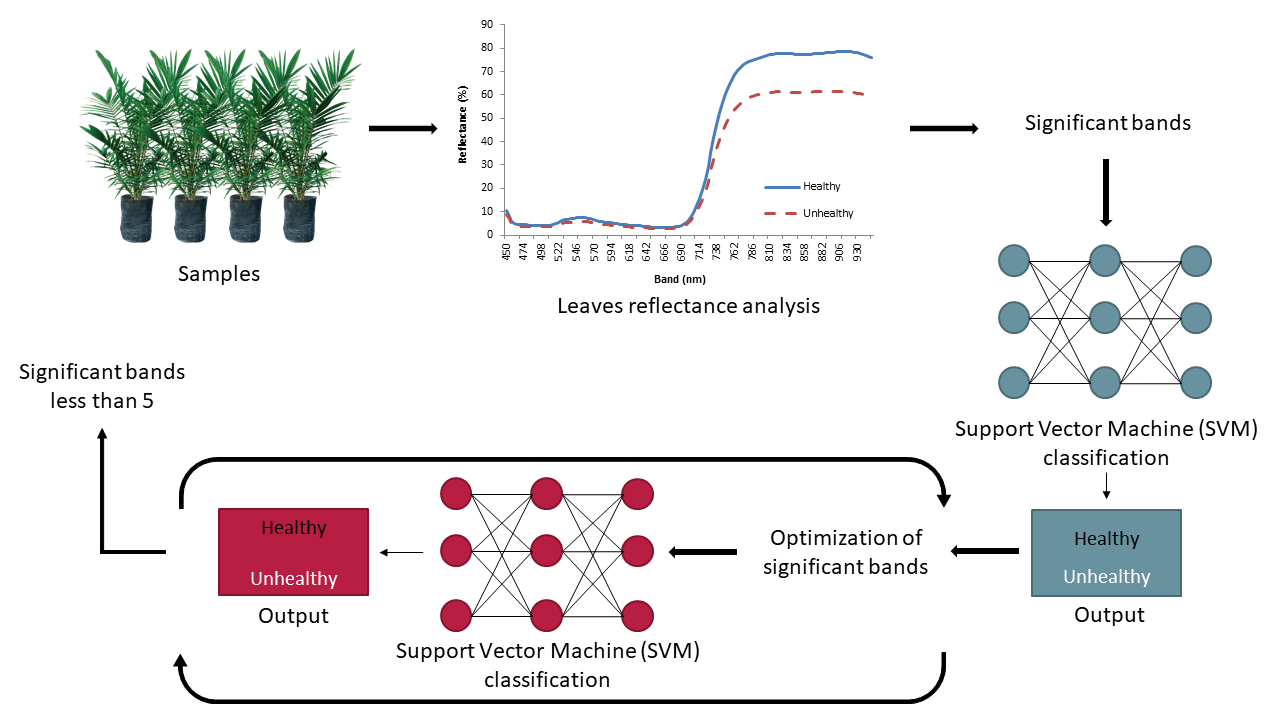
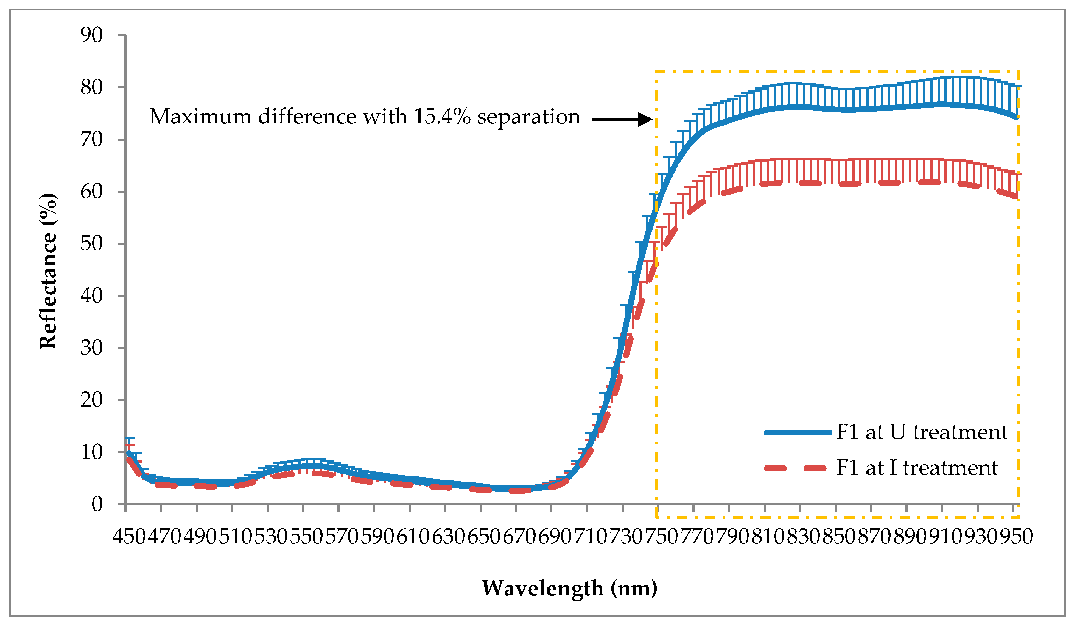
The reflectance pattern generated by I seedlings was typical for diseased plants, with lower reflectance in the NIR spectrum due to the destruction of xylem, which thus reduced the chlorophyll pigments and also caused water deficiency. According to Liaghat et al. [67], changes of reflectance in the NIR spectrum during a stress period were more evident than changes in the visible spectrum, since NIR could penetrate deeper through the leaf pigments compared to the visible wavelengths. The changes in NIR were due to the rupture of the mesophyll cell wall [62,77,78,79] which caused higher absorbance and lower reflectance of NIR. This result agreed with the findings by Ausmus and Hilty [80], where healthy maize dwarf mosaic virus-infected leaves showed significant differences in the NIR range even before the development of the physical symptoms, where the NIR reflectance of healthy leaves was higher than infected leaves.
In this study, the U seedlings reflected a slightly higher light level compared to the I seedlings in the visible range. This pattern was contrary to the spectral signature of healthy plants studied by other researchers that agreed healthy plants normally have lower reflectance than a diseased plant in the visible range, especially for green (520 to 560 nm) due to the higher chlorophyll content of the leaves. Nevertheless, the pattern shown in this study was similar to the study conducted by Shafri et al. [48] where the healthy seedlings yielded higher reflectance than G. boninense-infected seedlings in the green wavelengths. Therefore, this reflectance pattern might be a unique spectral signature for oil palm seedlings, since each plant has a specific spectral signature. Furthermore, according to Schmidt and Skidmore [81], different types of vegetation have spectral reflectance that is statistically significant in various spectral regions.
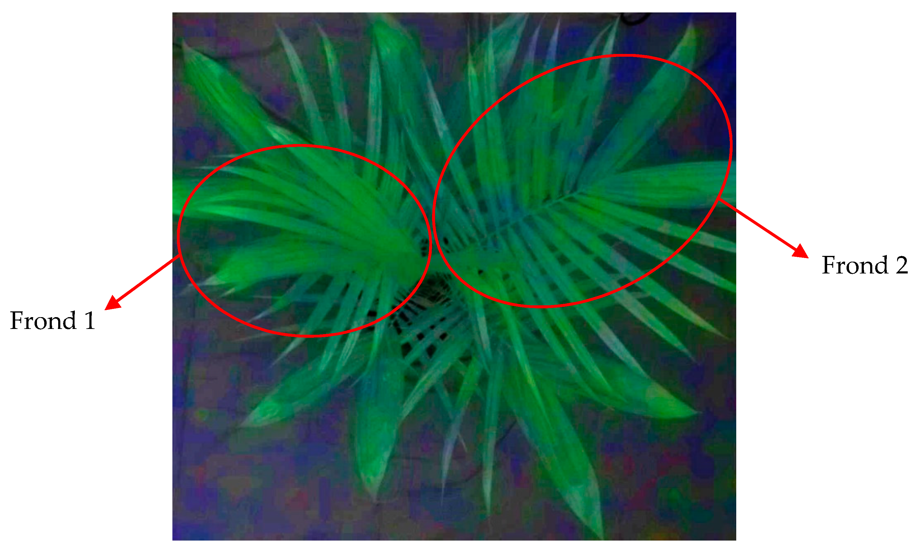
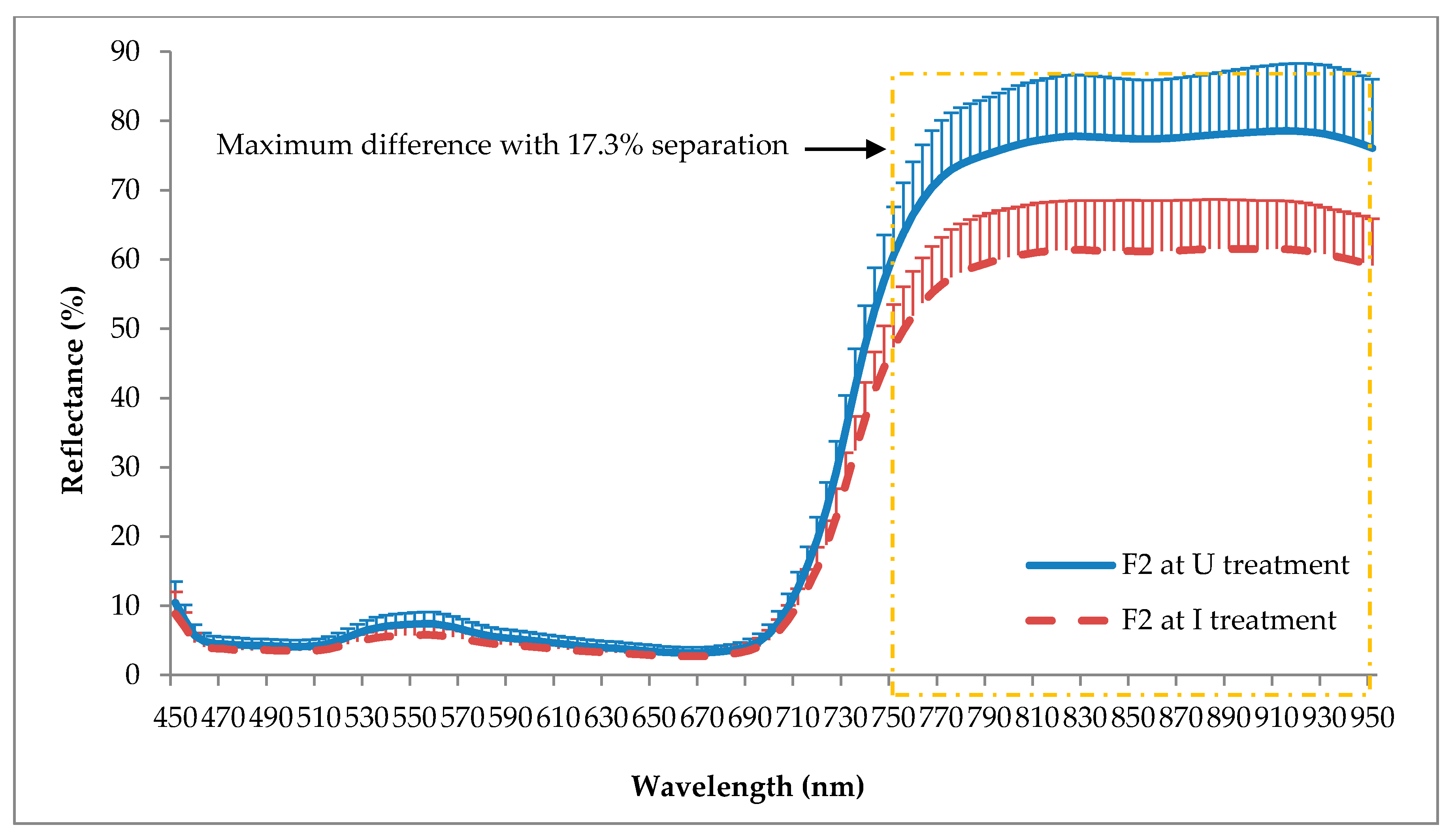
Although the reflectance patterns of the U and I seedlings of F1 and F2 were almost similar, the U of F2 produced a slightly higher reflectance than the U of F1 throughout the spectrum. This may indicate that the older leaves generated higher reflectance than the younger leaves. This idea was supported by Rapaport et al. [82] who found increases of NIR reflectance of Cabernet Sauvignon in the second week when the fourth leaf (young) of the control treatment moved to the eighth nodal position (old leaf position) and concluded that age variability mainly influenced the differences in reflectance spectra. Contrarily, Ahmadi et al. [62] presented average reflectance curves of healthy oil palms where frond 17 (old) produced lower NIR reflectance than frond 9 (young) during the first data collection. However, for the second data collection (8 months later), the NIR reflectance of frond 17 and 9 were almost similar. These reflectance spectra were not consistent with the first data collection.
By using the selected wavelengths of 800 to 950 nm, it was possible to obtain 100% classification accuracy in discriminating healthy and asymptomatic G. boninense-infected seedlings. The results also confirm that the prediction models developed using F1 generally had the most excellent accuracy of 100% when using 35 and 18 bands as input parameters. In addition, the accuracies attained by the SVM models showed that F12 was able to improve the accuracies of F2, which verified that both fronds could be used to detect the G. boninense infection in oil palm. This outcome agreed with Shafri et al. [48] who conducted a Maximum Likelihood classification using a combination of F1 and F2 to determine the health status of oil palm seedlings and achieved a net accuracy of 82% with a kappa coefficient of 0.73. Focusing on the similar type of input data used by Shafri et al. [48], i.e., F1 and F2, our method gave better accuracy with more than 90% at a different number of bands. Shafri et al. [48] used 24 significant bands (three green bands, 20 red bands and one NIR band) of first derivative spectra as input parameters. Our method that used the NIR spectrum performed well even at the small number of bands, i.e., nine bands with 94% accuracy. Reducing the number of bands has the advantages of being less complex and more economical. This promising result gave useful information in aerial-view applications such as when applying an unmanned aerial vehicle (UAV) for image acquisition since both fronds can be clearly seen from the top-view image and hence could expedite the detection of the G. boninense disease.
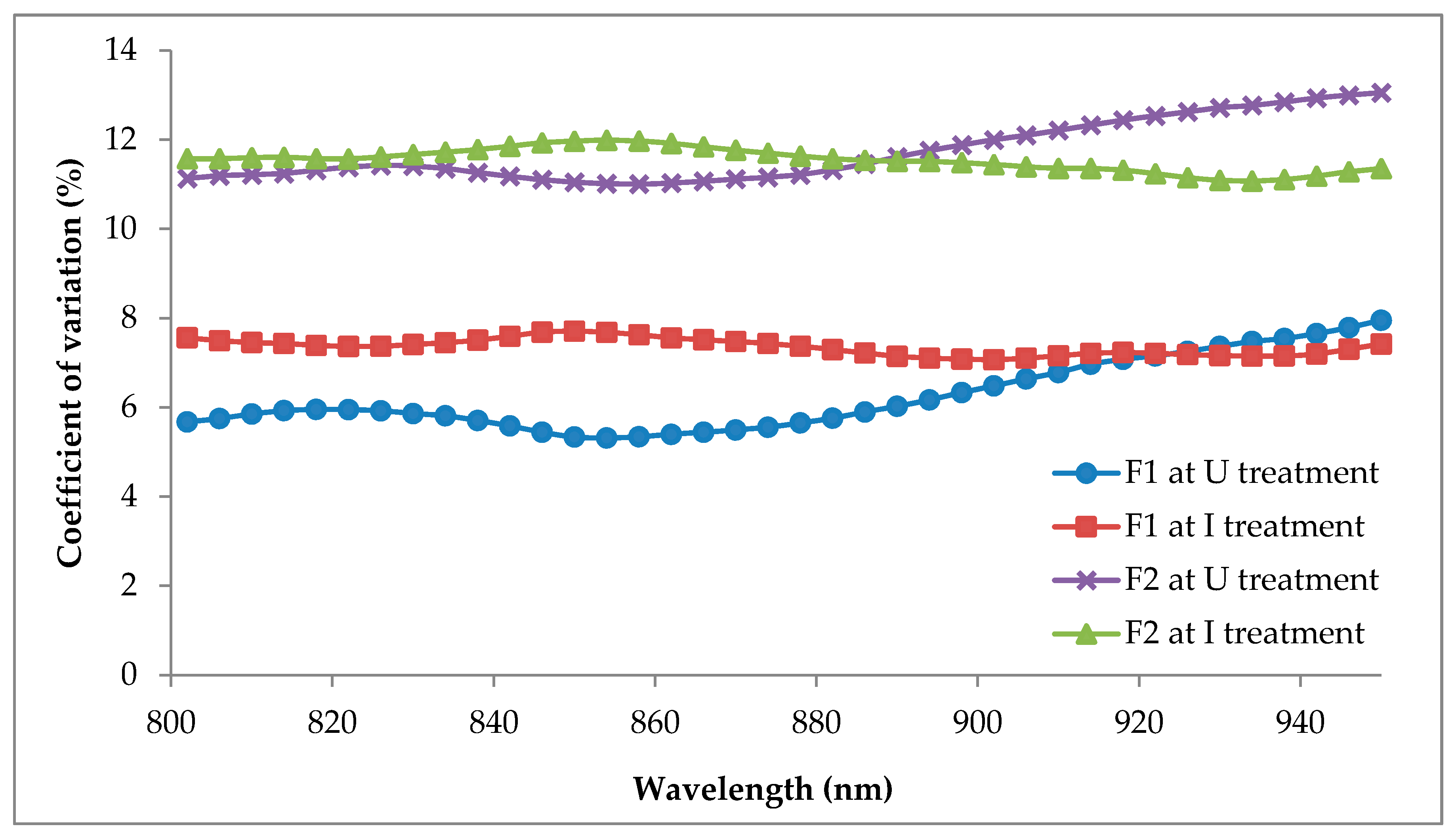
The F1 and F12 classification models produced robust results in contrast to the F2 classification models. For example, several SVM classifiers scored high classification accuracy when using the 35 and 18 (for F1 and F12), 9 and 5 (for F1), and 14 (for F12) bands which suggested that even a small number of input parameters could attain classification accuracies similar to a large number of input parameters. However, it depended on the type of classifiers used. Unlike the F2, the highest classification accuracy was only accomplished by Fine Gaussian SVM using 35 bands. The differences in the number of bands have no significant impact on the accuracy generated by the SVM classifiers. For example, nine bands were able to gain classification accuracies above 90% similar to 35, 18, and 14 bands when processed with F2. The distinct differences between the accuracy of F1 and F2 occurred due to the higher CV of F2, which indicate a higher dispersion of data in F2. In addition, Ahmadi et al. [62] claimed that younger fronds were more suitable to be used for the early detection of G. boninense infection since it has a better effect on classification accuracy than the older fronds due to its location on the top part of the crown.
Moreover, the results also present the importance of the kernel method, where Fine Gaussian SVM outperformed Linear SVM with higher classification accuracy in 14 bands of F2, and nine bands of F12, while Medium Gaussian SVM could attain similar accuracies as Linear SVM except when using nine bands of F2. In contrast, Coarse Gaussian SVM obtained less accuracy than the Linear SVM in all bands of F2 but higher in nine bands of F12. Therefore, it showed that the Gaussian RBF classifiers could provide a much better classification than the linear kernel SVM by using the appropriate kernel scale. However, for the polynomial kernel, Quadratic SVM yielded higher classification accuracy than Cubic SVM in F2 and F12, whereas Cubic SVM scored higher classification accuracy than Quadratic SVM in F1. Therefore, this indicated that the performance of SVM-based classification models was highly affected by the different types of data and kernel function, as the kernel effect depended on the data used. For example, F1 data could be optimized to five bands with classification accuracies scoring still above 85% for all SVM classifiers. In comparison, F2 and F12 could only be optimized to 14 bands since the Cubic SVM gave lower accuracy than 85% for both data sets.

5. Conclusions

NIR reflectance showed significant differences between the U and I seedlings. G. boninense infection can be detected at an early stage even though there are no physical symptoms of the disease by using SVM classifiers with a varying number of NIR bands. The reflectance spectra of the F1 frond yielded 100% classification accuracy for all SVM kernel functions using 35 and 18 NIR bands. In contrast, the F2 and F12 fronds achieved the highest classification accuracy of 93% when using Fine Gaussian SVM at 35 NIR bands and 95% when using Gaussian RBF and linear kernel at 35, 18, and 14 NIR bands, respectively. Since F12 produced higher classification accuracy than F2, it could be concluded that F12 would be better used for early detection of G. boninense infection in oil palm when using aerial images because there is no need to separate between F1 and F2 during the pre-processing data stage. Next, it was observed that a high number of bands achieved high classification accuracy while a small number of bands obtained slightly less accuracy. In addition, the optimized Gaussian RBF kernel, i.e., Fine Gaussian SVM could perform excellently compared to the Linear SVM and other classifiers in terms of the classification accuracy produced. However, it depended on the number of bands and fronds used.
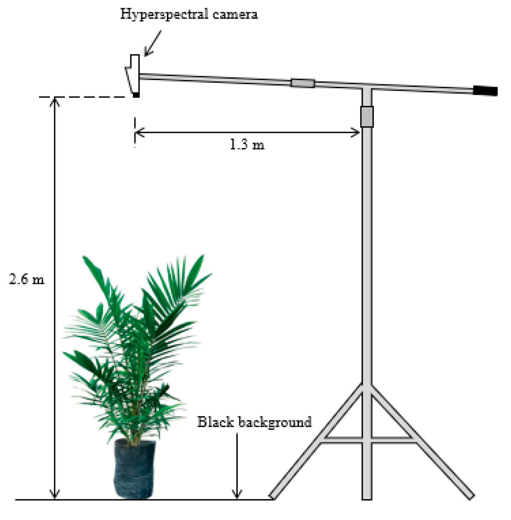
For future work, the developed method in this research could be tested in an open environment to confirm its reliability for field application. Even the camera could be calibrated before every image acquisition to avoid error due to illumination. However, careful consideration needs to be taken when dealing with sun angle, shadow and weather conditions. In addition, the inoculation period of oil palm seedlings could be shortened to less 10 months to check the ability to detect the earliest infection of G. boninense. Next, research could also be implemented for different types of oil palm varieties to test their tolerance towards G. boninense infection and its effects on spectral reflectance.

Author Contributions

Formal analysis, A.N.N.A. and S.K.B.; investigation, A.N.N.A. and N.A.H.; writing—original draft preparation, A.N.N.A.; writing—review and editing, S.K.B.; supervision, M.J., F.M.M. and I.Y. All authors have read and agreed to the published version of the manuscript.

Funding

This research was funded by the Ministry of Higher Education Malaysia and Universiti Putra Malaysia (UPM), research number LRGS-NANOMITE/5526305.

Conflicts of Interest

The authors declare no conflict of interest.

References

  1. Sanderson, F.R. An insight into spore dispersal of Ganoderma boninense on oil palm. Mycopathologia 2005, 159, 139–141. [Google Scholar] [CrossRef] [PubMed]
  2. Flood, J.; Hasan, Y.; Turner, P.D.; O’Grady, E.B. The spread of Ganoderma from infective sources in the field and its implication for management of the disease in oil palm. In Ganoderma Diseases of Perennial Crops; Flood, J., Bridge, P.D., Holderness, M., Eds.; CABI: New York, NY, USA, 2000; pp. 101–112. [Google Scholar]
  3. Subagio, A.; Foster, H.L. Implications of Ganoderma disease on loss in stand and yield production of oil palm in North Sumatra. In Proceedings of the MAPPS Conference 2003, Kuala Lumpur, Malaysia, 11 August 2003; Malaysian Plant Protection Society: Kuching, Malaysia, 2003. [Google Scholar]
  4. Roslan, A.; Idris, A.S. Economic impact of Ganoderma incidence on Malaysian oil palm plantation—A case study in Johor. Oil Palm Ind. Econ. J. 2012, 12, 24–30. [Google Scholar]
  5. Idris, A.S.; Kushairi, D.; Ariffin, D.; Basri, M.W. Technique for inoculation of oil palm germinated seeds with Ganoderma. Mpob Inf. Ser. 2006, 314, 1–4. [Google Scholar]
  6. Meor, M.S.Y.; Khalid, M.A.; Idris, A.S. Identification of basal stem rot disease in local palm oil by microfocus XRF. J. Nucl. Relat. Technol. 2009, 6, 282–287. [Google Scholar]
  7. Naher, L.; Siddiquee, S.; Yusuf, U.K.; Mondal, M.M.A. Issues of Ganoderma spp. and basal stem rot disease management in oil palm. Am. J. Agric. Sci. 2015, 2, 103–107. [Google Scholar]
  8. Sariah, M.; Hussin, M.Z.; Miller, R.N.G.; Holderness, M. Pathogenicity of Ganoderma boninense tested by inoculation of oil palm seedlings. Plant Pathol. 1994, 43, 507–510. [Google Scholar] [CrossRef]
  9. Haniff, M.H.; Ismail, S.; Idris, A.S. Gas exchange responses of oil palm to Ganoderma boninense infection. Asian J. Plant Sci. 2005, 4, 438–444. [Google Scholar]
  10. Natarajan, S.; Bhaskaran, R.; Shanmugan, N. Preliminary studies to develop techniques for early detection of Thanjavur wilt in coconut. Indian Coconut J. (India) 1986, 17, 3–6. [Google Scholar]
  11. Ariffin, D.; Idris, A.S.; Marzuki, A. Spread of Ganoderma boninense and vegetative compatibility studies of a single field palm isolates. In Proceedings of the 1996 PORIM International Palm Oil Congress (Agriculture), Kuala Lumpur, Malaysia, 23–28 September 1996; Palm Oil Research Institute Malaysia: Kuala Lumpur, Malaysia, 1996. [Google Scholar]
  12. Darmono, T.W. Detection of basal stem rot disease of oil palm using polyclonal antibody. Menara Perkeb. 1999, 67, 32–39. [Google Scholar]
  13. Madihah, A.Z.; Idris, A.S.; Rafidah, A.R. Polyclonal antibodies of Ganoderma boninense isolated from Malaysian oil palm for detection of basal stem rot disease. Afr. J. Biotechnol. 2014, 13, 3455–3463. [Google Scholar] [CrossRef] [Green Version]
  14. Idris, A.S.; Rafidah, A.R. Polyclonal Antibody for Detection of Ganoderma; MPOB Information Series No.405; MPOB: Bandar Baru Bangi, Malaysia, 2008. [Google Scholar]
  15. Kandan, A.; Radjacommare, R.; Ramanathan, A.; Raguchander, T.; Balasubramanian, P.; Samiyappan, R. Molecular biology of Ganoderma pathogenicity and diagnosis in coconut seedlings. Folia Microbiol. 2009, 54, 147–152. [Google Scholar] [CrossRef] [PubMed]
  16. Utomo, C.; Niepold, F. Development of diagnostic methods for detecting Ganoderma-infected oil palms. J. Phytopathol. 2000, 148, 507–514. [Google Scholar] [CrossRef]
  17. Idris, A.S.; Yamaoka, M.; Hayakawa, S.; Basri, M.W.; Noorhasimah, I.; Ariffin, D. PCR Technique for Detection of Ganoderma; MPOB Information Series No.188; MPOB: Bandar Baru Bangi, Malaysia, 2003. [Google Scholar]
  18. Markom, M.A.; Shakaff, A.M.; Adom, A.H.; Ahmad, M.N.; Hidayat, W.; Abdullah, A.H.; Fikri, N.A. Intelligent electronic nose system for basal stem rot disease detection. Comput. Electron. Agric. 2009, 66, 140–146. [Google Scholar] [CrossRef]
  19. Abdullah, A.H.; Adom, A.H.; Ahmad, M.N.; Saad, M.A.; Tan, E.S.; Fikri, N.A.; Zakaria, A. Electronic nose system for Ganoderma detection. Sens. Lett. 2011, 9, 353–358. [Google Scholar] [CrossRef]
  20. Abdullah, J.; Hassan, H.; Shari, M.R.; Mohd, S.; Mustapha, M.; Mahmood, A.A.; Hamid, N.H. GammaScorpion: Mobile gamma-ray tomography system for early detection of basal stem rot in oil palm plantations. Opt. Eng. 2013, 52, 036502. [Google Scholar] [CrossRef]
  21. Khairunniza-Bejo, S.; Vong, C.N. Detection of basal stem rot (BSR) infected oil palm tree using laser scanning data. Agric. Agric. Sci. Procedia 2014, 2, 156–164. [Google Scholar] [CrossRef] [Green Version]
  22. Azuan, N.H.; Khairunniza-Bejo, S.; Abdullah, A.F.; Kassim, M.S.M.; Ahmad, D. Analysis of changes in oil palm canopy architecture from basal stem rot using terrestrial laser scanner (TLS). Plant Dis. 2019, 103, 3218–3225. [Google Scholar] [CrossRef] [Green Version]
  23. Husin, N.A.; Khairunniza-Bejo, S.; Abdullah, A.F.; Kassim, M.S.; Ahmad, D.; Azmi, A.N. Application of ground-based LiDAR for analysing oil palm canopy properties on the occurrence of basal stem rot (BSR) Disease. Sci. Rep. 2020, 10, 1–16. [Google Scholar] [CrossRef] [Green Version]
  24. Bravo, C.; Moshou, D.; West, J.; McCartney, A.; Ramon, H. Early disease detection in wheat fields using spectral reflectance. Biosyst. Eng. 2003, 84, 137–145. [Google Scholar] [CrossRef]
  25. Yang, Z.; Rao, M.N.; Elliott, N.C.; Kindler, S.D.; Popham, T.W. Differentiating stress induced by greenbugs and Russian wheat aphids in wheat using remote sensing. Comput. Electron. Agric. 2009, 67, 64–70. [Google Scholar] [CrossRef]
  26. Kumar, A.; Lee, W.S.; Ehsani, R.J.; Albrigo, L.G.; Yang, C.; Mangan, R.L. Citrus greening disease detection using aerial hyperspectral and multispectral imaging techniques. J. Appl. Remote Sens. 2012, 6, 063542. [Google Scholar]
  27. Zhang, J.; Pu, R.; Huang, W.; Yuan, L.; Luo, J.; Wang, J. Using in-situ hyperspectral data for detecting and discriminating yellow rust disease from nutrient stresses. Field Crops Res. 2012, 134, 165–174. [Google Scholar] [CrossRef]
  28. Alexander, A.; Dayou, J.; Sipaut, C.S.; ChongKhim, P.; LeePing, C. Some interpretations on FTIR results for the detection of Ganoderma boninense in oil palm tissue. Adv. Environ. Biol. 2014, 8, 30–32. [Google Scholar]
  29. Susič, N.; Žibrat, U.; Širca, S.; Strajnar, P.; Razinger, J.; Knapič, M.; Stare, B.G. Discrimination between abiotic and biotic drought stress in tomatoes using hyperspectral imaging. Sens. Actuators Chem. 2018, 273, 842–852. [Google Scholar] [CrossRef] [Green Version]
  30. Ye, D.; Sun, L.; Tan, W.; Che, W.; Yang, M. Detecting and classifying minor bruised potato based on hyperspectral imaging. Chemom. Intell. Lab. Syst. 2018, 177, 129–139. [Google Scholar] [CrossRef]
  31. Li, B.; Xu, X.; Zhang, L.; Han, J.; Bian, C.; Li, G.; Jin, L. Above-ground biomass estimation and yield prediction in potato by using UAV-based RGB and hyperspectral imaging. ISPRS J. Photogramm. Remote Sens. 2020, 162, 161–172. [Google Scholar] [CrossRef]
  32. Jiang, H.; Zhang, C.; He, Y.; Chen, X.; Liu, F.; Liu, Y. Wavelength selection for detection of slight bruises on pears based on hyperspectral imaging. Appl. Sci. 2016, 6, 450. [Google Scholar] [CrossRef] [Green Version]
  33. Rivera, N.V.; Gómez-Sanchis, J.; Chanona-Pérez, J.; Carrasco, J.J.; Millán-Giraldo, M.; Lorente, D.; Blasco, J. Early detection of mechanical damage in mango using NIR hyperspectral images and machine learning. Biosyst. Eng. 2014, 122, 91–98. [Google Scholar] [CrossRef]
  34. Pantazi, X.E.; Tamouridou, A.A.; Alexandridis, T.K.; Lagopodi, A.L.; Kontouris, G.; Moshou, D. Detection of Silybum marianum infection with Microbotryum silybum using VNIR field spectroscopy. Comput. Electron. Agric. 2017, 137, 130–137. [Google Scholar] [CrossRef]
  35. Guo, C.; Guo, X. Estimating leaf chlorophyll and nitrogen content of wetland emergent plants using hyperspectral data in the visible domain. Spectrosc. Lett. 2016, 49, 180–187. [Google Scholar] [CrossRef]
  36. Krezhova, D.; Velichkova, K.; Petrov, N.; Maneva, S. The effect of plant diseases on hyperspectral leaf reflectance and biophysical parameters. In Proceedings of the 5th International Conference on Radiation and Application in Various Fields of Research (RAD-2017), Budva, Montenegro, 11–16 June 2017. [Google Scholar]
  37. Lowe, A.; Harrison, N.; French, A.P. Hyperspectral image analysis techniques for the detection and classification of the early onset of plant disease and stress. Plant Methods 2017, 13, 80. [Google Scholar] [CrossRef] [PubMed]
  38. Jin, J.; Wang, Q. Hyperspectral indices based on first derivative spectra closely trace canopy transpiration in a desert plant. Ecol. Inform. 2016, 35, 1–8. [Google Scholar] [CrossRef]
  39. Peng, Y.; Fan, M.; Song, J.; Cui, T.; Li, R. Assessment of plant species diversity based on hyperspectral indices at a fine scale. Sci. Rep. 2018, 8, 1–11. [Google Scholar] [CrossRef] [PubMed] [Green Version]
  40. Rumpf, T.; Mahlein, A.K.; Steiner, U.; Oerke, E.C.; Dehne, H.W.; Plümer, L. Early detection and classification of plant diseases with support vector machines based on hyperspectral reflectance. Comput. Electron. Agric. 2010, 74, 91–99. [Google Scholar] [CrossRef]
  41. Nagasubramanian, K.; Jones, S.; Sarkar, S.; Singh, A.K.; Singh, A.; Ganapathysubramanian, B. Hyperspectral band selection using genetic algorithm and support vector machines for early identification of charcoal rot disease in soybean stems. Plant Methods 2018, 14, 86. [Google Scholar] [CrossRef] [PubMed]
  42. Helmi, Z.; Mohanad, S.E. Quantitative performance of spectral indices in large scale plant health analysis. Am. J. Agric. Biol. Sci. 2009, 4, 187–191. [Google Scholar]
  43. Shafri, H.Z.; Hamdan, N. Hyperspectral imagery for mapping disease infection in oil palm plantation using vegetation indices and red-edge techniques. Am. J. Appl. Sci. 2009, 6, 1031. [Google Scholar]
  44. Shafri, H.Z.M.; Hamdan, N.; Izzuddin Anuar, M. Detection of stressed oil palms from an airborne sensor using optimized spectral indices. Int. J. Remote Sens. 2012, 33, 4293–4311. [Google Scholar] [CrossRef]
  45. Izzuddin, M.A.; Idris, A.S.; Nisfariza, N.M.; Ezzati, B. Spectral based analysis of airborne hyperspectral remote sensing image for detection of Ganoderma disease in oil palm. In Proceedings of the 2015 International Conference on Biological and Environmental Science (BIOES 2015), Phuket, Thailand, 1–2 October 2015; pp. 13–20. [Google Scholar]
  46. Izzuddin, M.A.; Nisfariza, M.N.; Ezzati, B.; Idris, A.S.; Steven, M.D.; Boyd, D. Analysis of airborne hyperspectral image using vegetation indices, red edge position and continuum removal for detection of Ganoderma disease in oil palm. J. Oil Palm Res. 2018, 30, 416–428. [Google Scholar]
  47. Shafri, H.Z.M.; Anuar, M.I. Hyperspectral signal analysis for detecting disease infection in oil palms. In Proceedings of the International Conference on Computer and Electrical Engineering 2008, Phuket, Thailand, 20–22 December 2008; IEEE: New York, NY, USA, 2008. [Google Scholar]
  48. Shafri, H.Z.; Anuar, M.I.; Seman, I.A.; Noor, N.M. Spectral discrimination of healthy and Ganoderma-infected oil palms from hyperspectral data. Int. J. Remote Sens. 2011, 32, 7111–7129. [Google Scholar] [CrossRef]
  49. Chung, C.L.; Huang, K.J.; Chen, S.Y.; Lai, M.H.; Chen, Y.C.; Kuo, Y.F. Detecting Bakanae disease in rice seedlings by machine vision. Comput. Electron. Agric. 2016, 121, 404–411. [Google Scholar] [CrossRef]
  50. Ebrahimi, M.A.; Khoshtaghaza, M.H.; Minaei, S.; Jamshidi, B. Vision-based pest detection based on SVM classification method. Comput. Electron. Agric. 2017, 137, 52–58. [Google Scholar] [CrossRef]
  51. Ramos, P.J.; Prieto, F.A.; Montoya, E.C.; Oliveros, C.E. Automatic fruit count on coffee branches using computer vision. Comput. Electron. Agric. 2017, 137, 9–22. [Google Scholar] [CrossRef]
  52. Zhang, M.; Li, C.; Yang, F. Classification of foreign matter embedded inside cotton lint using short wave infrared (SWIR) hyperspectral transmittance imaging. Comput. Electron. Agric. 2017, 139, 75–90. [Google Scholar] [CrossRef]
  53. Kaur, P.; Pannu, H.S.; Malhi, A.K. Plant disease recognition using fractional-order Zernike moments and SVM classifier. Neural Comput. Appl. 2019, 31, 8749–8768. [Google Scholar] [CrossRef]
  54. Santoso, H.; Tani, H.; Wang, X. Random Forest classification model of basal stem rot disease caused by Ganoderma boninense in oil palm plantations. Int. J. Remote Sens. 2017, 38, 4683–4699. [Google Scholar] [CrossRef]
  55. Santoso, H.; Tani, H.; Wang, X.; Prasetyo, A.E.; Sonobe, R. Classifying the severity of basal stem rot disease in oil palm plantations using WorldView-3 imagery and machine learning algorithms. Int. J. Remote Sens. 2019, 40, 7624–7646. [Google Scholar] [CrossRef]
  56. Khaled, A.Y.; Abd Aziz, S.; Bejo, S.K.; Nawi, N.M.; Jamaludin, D.; Ibrahim, N.U.A. A comparative study on dimensionality reduction of dielectric spectral data for the classification of basal stem rot (BSR) disease in oil palm. Comput. Electron. Agric. 2020, 170, 105288. [Google Scholar] [CrossRef]
  57. Shafri, H.Z.M.; Anuar, M.I.; Saripan, M.I. Modified vegetation indices for Ganoderma disease detection in oil palm from field spectroradiometer data. J. Appl. Remote Sens. 2009, 3, 033556. [Google Scholar]
  58. Tawfik, O.; Shafri, H.M.; Mohammed, A.A. Disease detection from field spectrometer data. Iium Eng. J. 2013, 14, 133–143. [Google Scholar] [CrossRef]
  59. Izzuddin, M.A.; Seman Idris, A.; Nisfariza, M.N.; Nordiana, A.A.; Shafri, H.Z.M.; Ezzati, B. The development of spectral indices for early detection of Ganoderma disease in oil palm seedlings. Int. J. Remote Sens. 2017, 38, 6505–6527. [Google Scholar] [CrossRef]
  60. Nisfariza, M.N.; Idris, A.S.; Shafri, Z.H.; Steven, M.; Boyd, D. Hyperspectral derivative band ratios of oil palm stress associated with Ganoderma basal stem rot disease. In Proceedings of the Malaysia Remote Sensing Society (MRSS) 2010, Kuala Lumpur, Malaysia, 28–29 April 2010. [Google Scholar]
  61. Nisfariza, M.N.; Shafri, Z.H.; Idris, A.; Steven, M.; Boyd, D.; Mior, M. Hyperspectral sensing possibilities using continuum removal index in early detection of Ganoderma in oil palm plantation. In Proceedings of the World Engineering Congress 2010, Conference on Geomatics and Geographical Information Science, Kuching, Sarawak, Malaysia, 2–5 August 2010; pp. 233–239. [Google Scholar]
  62. Ahmadi, P.; Muharam, F.M.; Ahmad, K.; Mansor, S.; Abu Seman, I. Early detection of Ganoderma basal stem rot of oil palms using artificial neural network spectral analysis. Plant Dis. 2017, 101, 1009–1016. [Google Scholar] [CrossRef] [PubMed] [Green Version]
  63. Lelong, C.C.; Roger, J.M.; Bregand, S.; Dubertret, F.; Lanore, M.; Sitorus, N.A.; Caliman, J.P. Discrimination of fungal disease infestation in oil-palm canopy hyperspectral reflectance data. In Proceedings of the First Workshop on Hyperspectral Image and Signal Processing: Evolution in Remote Sensing, Grenoble, France, 26–28 August 2009; IEEE: New York, NY, USA, 2009. [Google Scholar]
  64. Lelong, C.C.; Roger, J.M.; Brégand, S.; Dubertret, F.; Lanore, M.; Sitorus, N.A.; Caliman, J.P. Evaluation of oil-palm fungal disease infestation with canopy hyperspectral reflectance data. Sensors 2010, 10, 734–747. [Google Scholar] [CrossRef] [PubMed]
  65. Liaghat, S.; Mansor, S.; Ehsani, R.; Shafri, H.Z.M.; Meon, S.; Sankaran, S. Mid-infrared spectroscopy for early detection of basal stem rot disease in oil palm. Comput. Electron. Agric. 2014, 101, 48–54. [Google Scholar] [CrossRef]
  66. Dayou, J.; Alexander, A.; Sipaut, C.S.; Phin, C.K.; Chin, L.P. On the possibility of using FTIR for detection of Ganoderma boninense in infected oil palm tree. J. Adv. Agric. Environ. Eng. 2014, 1, 161–163. [Google Scholar]
  67. Liaghat, S.; Ehsani, R.; Mansor, S.; Shafri, H.Z.; Meon, S.; Sankaran, S.; Azam, S.H. Early detection of basal stem rot disease (Ganoderma) in oil palms based on hyperspectral reflectance data using pattern recognition algorithms. Int. J. Remote Sens. 2014, 35, 3427–3439. [Google Scholar] [CrossRef]
  68. Izzuddin, M.A.; Idris, A.S.; Wahid, O.; Nishfariza, M.N.; Shafri, H.Z.M. Field Spectroscopy for Detection of Ganoderma Disease in Oil Palm; MPOB Information Series No.532; MPOB: Bandar Baru Bangi, Malaysia, 2013. [Google Scholar]
  69. Kamil, N.N.; Omar, S.F. Climate variability and its impact on the palm oil industry. Oil Palm Ind. Econ. J. 2016, 16, 18–30. [Google Scholar]
  70. Naidu, Y.; Siddiqui, Y.; Rafii, M.Y.; Saud, H.M.; Idris, A.S. Inoculation of oil palm seedlings in Malaysia with white-rot hymenomycetes: Assessment of pathogenicity and vegetative growth. Crop Prot. 2018, 110, 146–154. [Google Scholar] [CrossRef]
  71. Asaari, M.S.M.; Mishra, P.; Mertens, S.; Dhondt, S.; Inzé, D.; Wuyts, N.; Scheunders, P. Close-range hyperspectral image analysis for the early detection of stress responses in individual plants in a high-throughput phenotyping platform. ISPRS J. Photogramm. Remote Sens. 2018, 138, 121–138. [Google Scholar] [CrossRef]
  72. Wilcox, R.R. A fundamental problem. In Fundamentals of Modern Statistical Methods: Substantially Improving Power and Accuracy, 2nd ed.; Springer: New York, NY, USA, 2010; pp. 109–126. [Google Scholar]
  73. Kwak, S.K.; Kim, J.H. Statistical data preparation: Management of missing values and outliers. Korean J. Anesthesiol. 2017, 70, 407. [Google Scholar] [CrossRef]
  74. Izzati, M.Z.N.A.; Abdullah, F. Disease suppression in Ganoderma-infected oil palm seedlings treated with Trichoderma harzianum. Plant Prot. Sci. 2008, 44, 101–107. [Google Scholar] [CrossRef] [Green Version]
  75. Kok, S.; Goh, Y.; Tung, H.; Goh, K.; Wong, W.; Goh, Y. In vitro growth of Ganoderma boninense isolates on novel palm extract medium and virulence on oil palm (Elaeis guineensis) seedlings. Malays. J. Microbiol. 2013, 9, 33–42. [Google Scholar]
  76. Lim, S.; Kim, S.H.; Kim, Y.; Cho, Y.S.; Kim, T.Y.; Jeong, W.K.; Sohn, J.H. Coefficient of Variance as Quality Criterion for Evaluation of Advanced Hepatic Fibrosis Using 2D Shear-Wave Elastography. J. Ultrasound Med. 2018, 37, 355–362. [Google Scholar] [CrossRef] [PubMed] [Green Version]
  77. Gausman, H.W. Reflectance of leaf components. Remote Sens. Environ. 1977, 6, 1–9. [Google Scholar] [CrossRef]
  78. Chappelle, E.W.; Kim, M.S.; McMurtrey, J.E., III. Ratio analysis of reflectance spectra (RARS): An algorithm for the remote estimation of the concentrations of chlorophyll a, chlorophyll b, and carotenoids in soybean leaves. Remote Sens. Environ. 1992, 39, 239–247. [Google Scholar] [CrossRef]
  79. Slaton, M.R.; Raymond Hunt, E., Jr.; Smith, W.K. Estimating near-infrared leaf reflectance from leaf structural characteristics. Am. J. Bot. 2001, 88, 278–284. [Google Scholar] [CrossRef] [PubMed]
  80. Ausmus, B.S.; Hilty, J.W. Reflectance studies of healthy, maize dwarf mosaic virus-infected, and Helminthosporium maydis-infected corn leaves. Remote Sens. Environ. 1971, 2, 77–81. [Google Scholar] [CrossRef]
  81. Schmidt, K.S.; Skidmore, A.K. Spectral discrimination of vegetation types in a coastal wetland. Remote Sens. Environ. 2003, 85, 92–108. [Google Scholar] [CrossRef]
  82. Rapaport, T.; Hochberg, U.; Rachmilevitch, S.; Karnieli, A. The effect of differential growth rates across plants on spectral predictions of physiological parameters. PLoS ONE 2014, 9, e88930. [Google Scholar] [CrossRef]
Figure 1. Illustration of hyperspectral image acquisition setup inside the greenhouse.
Remotesensing 12 03920 g001
Figure 2. Top view image of frond 1 (F1) and frond 2 (F2).
Remotesensing 12 03920 g002
Figure 3. Flowchart of optimization of band number for the reflectance dataset.
Remotesensing 12 03920 g003
Figure 4. (a) Physical condition of inoculated (I) seedlings that were sent for polymerase chain reaction (PCR) test at four weeks after inoculation; (b,c) brown discoloration at the bole of the seedlings.
Remotesensing 12 03920 g004
Figure 5. Condition of inoculated (I) seedling after 20 weeks of inoculation. There was no presence of basal stem rot (BSR) symptoms, i.e., fruiting bodies and yellowing of older leaves.
Remotesensing 12 03920 g005
Figure 6. Reflectance spectra of frond 1 (F1) at U and I treatments. Each value represents a mean of 202 and 248 sample points of U and I treatments, respectively. Vertical bars represent standard deviation.
Remotesensing 12 03920 g006
Figure 7. Spectral reflectance of frond 2 (F2) at U and I treatments. Each value represents a mean of 197 and 264 sample points of U and I treatments, respectively. Vertical bars represent standard deviation.
Remotesensing 12 03920 g007
Figure 8. Coefficient of variation (CV) of all significant band sample points of F1 and F2.
Remotesensing 12 03920 g008
Table 1. Summary of existing G. boninense detection methods for oil palm seedling and mature tree using hyperspectral remote sensing.
Applied SensorSpectral RangeStudy ScaleAge of SampleApplied MethodsSpecific Bands (nm)Accuracy
(%)
Reference
APOGEE spectroradiometer300 to 1000 nmNurseryn.a.Mann–Whitney U test and Jeffries–Matusita (JM) distance analysis460, 461.5, 462, 462.5, 467.5, 468.5, 469, 480, 480.5, 483, 488, 490.5, 500.5, 501.5, 503.5, 524, 524.5, 525, 525.5, 528.5, 567, 568, 700, 717, 718, 720.5 744, 744.5n.a.[47]
n.a.Mann–Whitney U test and Band ratio and Optimum index factor (OIF) and K-means clustering and Average silhouette width (ASW) plot 610.5, 738n.a.[57]
10 months oldAnalysis of variance (ANOVA) and JM distance analysis and Maximum Likelihood classification495, 495.5, 496, 651.5, 652, 652.5, 653, 653.5, 654, 654.5, 655, 655.5, 656, 656.5, 657, 657.5, 658, 658.5, 659, 659.5, 660, 660.5, 661, 90882[48]
n.a.Modified red-edge simple ratio and JM distance analysis460, 705 n.a.[58]
10 months oldANOVA and Band ratio and OIF and ASW495.5, 477.5n.a.[59]
GER 1500 handheld spectrometer350 to 1050 nmNursery n.a.Band ratio in relation with leaf chlorophyll content 702, 725n.a.[60]
Plantation5 and 17 years oldVegetation indices and Continuum removal400 to 550n.a.[61]
273 to 1100 nm12 years oldArtificial neural network550 to 56083.3
100
[62]
Unispec spectroradiometer310 to 1130 nmPlantationn.a.Partial least squares discriminant analysis (PLS-DA)n.a.92[63]
n.a.94[64]
FT-IR spectrometer255 to 2505 nmPlantation15 years oldPrinciple component analysis (PCA) and Multivariate pattern recognition classificationn.a.92[65]
2500 to 15,384 nmn.a.Spectral pattern analysis2857 to 3125, 6060 to 7194, 8000 to 10,000n.a.[28]
7692 to 10,000n.a.[66]
ASD field spectroradiometer325 to1075 nmPlantation15 years oldPCA and Multivariate pattern recognition classification and ANOVAn.a.97[67]
Spectroradiometer273.13 to 1099.57 nmPlantation2, 5 and 17 years oldSpectral pattern analysis using oil palm spectral analyzer system (OPSAS) software66280.8[68]
Airborne AISA sensor400 to 900 nmPlantationn.a.Vegetation indices 705, 75082.86[42]
n.a.Red-edge indices715, 734, 79184[43]
n.a.Vegetation indices and Minimum distance classification and Spectral angle mapper616, 73486[44]
5 years oldVegetation indices and Continuum removal 400 to 500 44.4[45]
401 to 997 nm17 years oldVegetation indices and Red-edge position and Continuum removal400 to 50044.4[46]
Table 2. Highest 30% significant bands of F1 and F2 as determined using spectral analysis and t-test statistical analysis.
Frond NumberTotal Significant BandsSignificant Bands (nm)
F135810 814 818 822 826 830 834 838 842 846 850 854 858 866 870 874 878 882 886 890 894 898 902 906 910 914 918 922 926 930 934 938 942 946 950
F235814 818 822 826 830 834 838 842 846 850 854 858 862 866 870 874 878 882 886 890 894 898 902 906 910 914 918 922 926 930 934 938 942 946 950
Table 3. Classification accuracies obtained using a different numbers of significant bands of F1.
Classification Accuracy (%)
Number of Significant Bands
Classifier351895
Linear SVM1001009999
Quadratic SVM1001009797
Cubic SVM1001009898
Fine Gaussian SVM1001009999
Medium Gaussian SVM1001009999
Coarse Gaussian SVM1001009797
Table 4. Significant band optimization of F1 as identified by classification accuracies of Support Vector Machine (SVM) classifiers.
Total Significant BandsSignificant Bands (nm)
18826 830 890 894 898 902 906 910 914 918 922 926 930 934 938 942 946 950
9918 922 926 930 934 938 942 946 950
5930 934 938 942 946
Table 5. Classification accuracies obtained using a different number of significant bands of F2.
Classification Accuracy (%)
Number of Significant Bands
Classifier3518914
Linear SVM92919191
Quadratic SVM90898890
Cubic SVM89894786
Fine Gaussian SVM93919192
Medium Gaussian SVM92919091
Coarse Gaussian SVM91909090
Table 6. Significant band optimization of F2 as identified by classification accuracies of SVM classifiers.
Total Significant BandsSignificant Bands (nm)
18882 886 890 894 898 902 906 910 914 918 922 926 930 934 938 942 946 950
9914 918 922 926 930 934 938 942 946
14898 902 906 910 914 918 922 926 930 934 938 942 946 950
Table 7. Significant band optimization of F12 as identified by classification accuracies of SVM classifiers.
Total Significant BandsSignificant Bands (nm)
35814 818 822 826 830 834 838 842 846 850 854 858 862 866 870 874 878 882 886 890 894 898 902 906 910 914 918 922 926 930 934 938 942 946 950
18826 886 890 894 898 902 906 910 914 918 922 926 930 934 938 942 946 950
9914 922 926 930 934 938 942 946 950
14898 902 906 910 914 918 922 926 930 934 938 942 946 950
Table 8. Classification accuracies obtained using a different number of significant bands of F12.
Classification Accuracy (%)
Number of Significant Bands
Classifier3518914
Linear SVM95959395
Quadratic SVM94939393
Cubic SVM94927889
Fine Gaussian SVM95959495
Medium Gaussian SVM95959495
Coarse Gaussian SVM95959494
Publisher’s Note: MDPI stays neutral with regard to jurisdictional claims in published maps and institutional affiliations.

