Parametric Models to Characterize the Phenology of the Lowveld Savanna at Skukuza, South Africa


1
Global Change Institute, University of the Witwatersrand, Braamfontein-Johannesburg 2050, South Africa
2
School of Animal, Plant and Environmental Sciences, University of the Witwatersrand, Braamfontein-Johannesburg 2050, South Africa
*
Author to whom correspondence should be addressed.
Remote Sens. 2020, 12(23), 3927; https://0-doi-org.brum.beds.ac.uk/10.3390/rs12233927
Submission received: 4 November 2020
/
Revised: 24 November 2020
/
Accepted: 24 November 2020
/
Published: 30 November 2020
(This article belongs to the Special Issue Recent Advances in Satellite Derived Global Land Product Validation)
Abstract
:Mathematical models, such as the logistic curve, have been extensively used to model the temporal evolution of biological processes, though other similarly shaped functions could be (and sometimes have been) used for this purpose. Most previous studies focused on agricultural regions in the Northern Hemisphere and were based on the Normalized Difference Vegetation Index (NDVI). This paper compares the capacity of four parametric double S-shaped models (Gaussian, Hyperbolic Tangent, Logistic, and Sine) to represent the seasonal phenology of an unmanaged, protected savanna biome in South Africa’s Lowveld, using the Fraction of Absorbed Photosynthetically Active Radiation (FAPAR) generated by the Multi-angle Imaging SpectroRadiometer-High Resolution (MISR-HR) processing system on the basis of data originally collected by National Aeronautics and Space Administration (NASA)’s Multi-angle Imaging SpectroRadiometer (MISR) instrument since 24 February 2000. FAPAR time series are automatically split into successive vegetative seasons, and the models are inverted against those irregularly spaced data to provide a description of the seasonal fluctuations despite the presence of noise and missing values. The performance of these models is assessed by quantifying their ability to account for the variability of remote sensing data and to evaluate the Gross Primary Productivity (GPP) of vegetation, as well as by evaluating their numerical efficiency. Simulated results retrieved from remote sensing are compared to GPP estimates derived from field measurements acquired at Skukuza’s flux tower in the Kruger National Park, which has also been operational since 2000. Preliminary results indicate that (1) all four models considered can be adjusted to fit an FAPAR time series when the temporal distribution of the data is sufficiently dense in both the growing and the senescence phases of the vegetative season, (2) the Gaussian and especially the Sine models are more sensitive than the Hyperbolic Tangent and Logistic to the temporal distribution of FAPAR values during the vegetative season, and, in particular, to the presence of long temporal gaps in the observational data, and (3) the performance of these models to simulate the phenology of plants is generally quite sensitive to the presence of unexpectedly low FAPAR values during the peak period of activity and to the presence of long gaps in the observational data. Consequently, efforts to screen out outliers and to minimize those gaps, especially during the rainy season (vegetation’s growth phase), would go a long way to improve the capacity of the models to adequately account for the evolution of the canopy cover and to better assess the relation between FAPAR and GPP.
1. Introduction
Vegetation regulates the carbon, energy, and water fluxes between the land and the atmosphere. Plants affect and respond to environmental and especially climatic conditions: they typically exhibit annual variations that match the seasonal evolution of temperature, water availability, solar irradiance, and other critical variables. Hence, they are also sensitive to climate fluctuations and changes. Phenology, the study of the seasonal evolution of plants, documents these variations and therefore provides evidence of the impact of climate change on the environment.
The Special Report on Emissions Scenarios (SRES) socio-economic CO2 emission scenario A2 of the Intergovernmental Panel on Climate Change (IPCC) provides a suitable context to evaluate conditions appropriate for the African continent. Under this scenario, Friedlingstein et al. [1] estimate that climate warming during the 21st century may reduce the net ecosystem productivity of the African continent and contribute up to 38% of the global climate-carbon cycle feedback. Properly characterizing vegetation’s phenology is crucial to document this evolution and to accurately parameterize the global land-atmosphere models [2]. In Southern Africa, air temperature near the ground has been increasing rapidly over the last five decades, at about twice the rate of the globally average surface temperature [3,4,5]. These changes, and associated fluctuations in the water cycle, are expected to have a significant impact on vegetation cover in the savanna biome, which occupies about 20% of the global land surface and 40% of Africa, according to Kutsch et al. [6].
Phenology, may have notable economic implications, as plant growth and development depend on the occurrence of essential weather events. Natural hazards, such as drought, flood, or fire, can jeopardize agricultural yield in a given year, or sometimes the sustainability of that economic activity. Phenology also informs on the land use and land cover type, providing useful information to manage societies, their economic systems, as well as to monitor the evolution of unmanaged areas, such as nature reserves. In the particular context of African ecosystems, savanna woody vegetation provides valuable ecosystem services [7,8], and the effective estimation of those resources is required to satisfy commitments to monitor and manage change within them [9].
Repeated observations of the density and diversity of woody plant species in African savanna regions suggest that variations in species composition and diversity are to a great extent also influenced by land use and anthropogenic disturbances [10]. In South Africa, and in the Lowveld in particular, rural households critically depend on fuelwood as a source of energy because of the prohibitive cost of gas and fuels. This socio-economic constraint has resulted in the exploitation of natural resources well beyond their capacity to regenerate, and therefore in the progressive deforestation of those environments. That situation leads to wood scarcity, as well as potential, and, in many cases, actual, conflicts over access to resources [11]; it is further exacerbated by a continuous exodus from rural areas to towns and cities, as well as by immigration from neighboring countries. As a result, settlements have been expanding and their environmental footprints have become more severe over time [12].
This paper leverages two resources to bear on this problem: remote sensing and field measurements to provide empirical evidence, and modeling to provide a rational framework for the interpretation of the data, despite the uncertainties inherent to all measurements, the irregular distribution of observations in time and missing data for various reasons. The aims of this methodological study were (i) to assess the suitability of four parametric double S-shaped functions (the Gaussian, Hyperbolic Tangent, or Logistic and Sine) to describe the phenology of savanna vegetation in the Lowveld, and (ii) to evaluate the capability of these data and models to account for the Gross Primary Productivity (GPP) of the vegetation around the Skukuza flux tower in South Africa’s Kruger National Park. This is of particular interest insofar as GPP is one of the contributing factors to estimate biomass accumulation or yield (in an agricultural context).
2. Study Area
The study site is centered on the Skukuza Eddy Covariance (EC) flux tower, which falls within the Lowveld in the north eastern part of Mpumalanga Province of South Africa (Figure 1). The Lowveld predominantly belongs to the large savanna biome, which covers one-third of the country. It is characterized by hot humid summers and mild dry winters. Summer rains occur between October and May across a west to east precipitation gradient, with a mean annual precipitation of 633 mm and mean annual temperature of 21 C [13]. The Lowveld’s dominant geology includes granite and gneiss with local gabbro intrusions [14]. The slopes and crests are characterized by a mixture of tall shrubland with few trees to moderately dense low woodland, and valleys dominated by dense thicket and open savanna. Vegetation distribution and density in the region are influenced by the rainfall gradient, geology, fire events, mega-herbivore browsing, cattle grazing, and the anthropogenic harvesting of wood [14,15]. Coppicing is prominent in areas which experience high levels of anthropogenic utilization [9]. Granite lowveld is the main vegetation unit in the area, with dominant tree species, including Terminalia sericea, Combretum zeyheri, Combretum apiculatum, Acacia nigrescens, dominant shrub species, including Dichrostachys cinerea and Grewia bicolor, and dominant grass species, including Pogonarthria squarrosa, Tricholaena monachne, Eragrostis rigidior, Panicum maximum, Aristida congesta, Digitaria eriantha, and Urochloa mossambicensis [13].
3. Data Collections
3.1. Satellite Measurements
3.1.1. Background
Observations of land surfaces from spaceborne platforms started in earnest in the early 1970s with the launch of the Earth Resources Technology Satellite (ERTS-1), subsequently renamed Landsat 1. In turn, the availability of multispectral measurements stimulated the development of methods to explore the significance and implications of those observations in practical applications. Rouse Jr. et al. [16] and [17] suggested that the ratio subsequently known as the Normalized Difference Vegetation Index (NDVI) was adequate to monitor “the vernal advancement and retrogradation (Green wave effect) of natural vegetation”, i.e., to monitor plant phenology as we understand it today. These events mark the start of a sustained effort to monitor the biosphere on the basis of space observations [18].
Over the past 50 years, significant progress has been achieved, and thousands of publications have been published [19], to characterize the state and evolution of plant canopies using observations of the reflectance of the planet in the solar spectral range. A full review of the literature dealing with the documentation of plant phenology on the basis of remote sensing measurements is outside the scope of this paper, but it is worth noting that progress has been achieved on multiple fronts:
- Major advances in understanding the processes of radiation transfer in complex environments resulted in the design and implementation of much improved algorithms. These aimed to effectively account for processes unrelated to vegetation (such as atmospheric clouds and aerosols, anisotropic effects, contributions to the measured signals due to variations in soil moisture, etc.) and to deliver reliable and accurate products to describe plant processes. The Fraction of Absorbed Photosynthetically Active Radiation (FAPAR) is a case in point, since it has been identified as one of the Essential Climate Variables (ECV) by the Global Climate Observing System (GCOS) [20]. These developments, in turn, led to a more quantitative representation of plant phenology (in [21,22,23]).
- The technology of measuring reflected radiation on spaceborne platforms has improved drastically, and is currently able to deliver up to hundreds of spectral bands at spatial resolutions of the order of tens of meters or less, sometimes on a daily basis, or to acquire data from multiple directions or in multiple polarizations. Data fusion with observations obtained with different instruments (e.g., LiDARs: see [24,25,26]) or in entirely different spectral regions (e.g., microwaves: see [27,28,29]) have also been explored, though much remains to be done in order to provide a holistic description of the environment, or of plant phenology in particular.
- Progress in the field of information technology delivered computing, networking and data archiving resources and capabilities orders of magnitude faster and more performant than even a few decades ago, and permitted the investigation of complex issues. Although the drive to acquire more and better observations continues unabated, the major bottleneck today concerns the actual analysis of those data and the extraction of useful information from the immense archives that have already been accumulated.
As a result, Earth observing satellites have yielded a long-term record of changes in vegetation photosynthetic activity, while ground-based eddy covariance measurements are providing automated, continuous and spatially averaged measures of carbon exchanges between the surface and the atmosphere. A global increase in ‘greening’ has been evidenced through remotely sensed indices, such as the Leaf Area Index (LAI) and Normalized Difference Vegetation Index (NDVI), suggesting an increase in the seasonally-integrated LAI of up to 25–50%, while less than 4% of the terrestrial areas exhibit a decrease of LAI [30]. Key drivers of phenology include temperature and photoperiod in the mid- and high-latitudes [2,31,32,33], while precipitation is regarded as the dominant driver in the tropics [34,35]. Satellite-based observations have been widely used to characterize the evolution of vegetation in the Northern Hemisphere, but other regions have received far less attention: A systematic review of phenology in Africa over the last decade reveals a recent increase in the number of phenological studies based on remote sensing but suggests that further investigations are needed across this continent, especially to focus on the relationship between climate and vegetation phenological changes [36].
Remote sensing research in the Lowveld has tended to focus on the use of mono-directional spectral measurements (from airborne and/or spaceborne sensors) which typically inform on the chemical composition of the targets (in [37,38,39,40]). More recently, sporadic airborne campaigns collecting Light Detection And Ranging (LiDAR) measurements have been used to document the structural properties of the vegetation canopies, e.g., to map the differences in canopy and sub-canopy cover height and distribution [26,41,42]. One of the main advantages of using LiDAR observations is the ability to capture sub-canopy structural changes specifically to examine bush encroachment, otherwise unattainable in mono-directional spectral measurements which only account for the aerial extent of the vegetation canopy [43]. Hybrid techniques combining structural observations from LiDAR and spectral measurements from hyperspectral and multispectral data sets demonstrate the ability to classify individual tree species [25,44]. To a lesser extent, Advanced Synthetic Aperture Radar (ASAR) measurements, which can observe the surface irrespective of the cloud cover, have been used to create regional scale baseline maps of savanna woody cover in the Lowveld [9]. Cutting-edge approaches utilizing LiDAR, ASAR, and hybrid-techniques are very interesting but infrequent and limited in geographical scope, constrained in part by the limited spatial coverage and the cost of obtaining the data sets.
3.1.2. Multi-Angular Observations
Anisotropy is typically considered a source of noise when analyzing remote sensing data from mono-angular spectral instruments but constitutes a definite advantage when analyzing measurement from multi-angular instruments [45]. Over the last three decades, the potential benefits of multi-angular observations have been recognized through the operation of innovative Earth Observation (EO) instruments, such as the Along-Track Scanning Radiometer (ATSR-1 and ATSR-2), the Polarization and Directionality of the Earth’s Reflectance (POLDER), and the Multi-angle Imaging SpectroRadiometer (MISR) instrument on-board National Aeronautics and Space Administration (NASA)’s Terra platform, which has been continuously operating since 24 February 2000. These instruments generate an improved characterization of the atmospheric and terrestrial environments because multi-angular measurements permit an accurate, quantitative decoupling of the distinct spectral and directional signatures of those geophysical media.
In this context, the recent availability of land surface products at the relatively high spatial resolution of 275 m generated by the MISR-HR (for High Resolution; version 2.01-0) processing system [46], about weekly over the period 2000–2018, offers new opportunities to explore the relation between surface properties and the fluxes of matter and energy in the environment. Appendix A summarizes the specifications of the MISR instrument and outlines the products generated by the MISR-HR processing system. Specifically, the Joint Research Centre-Two-stream Inversion Package (JRC-TIP) algorithm [47,48] derives the Fraction of Absorbed Photosynthetically Active Radiation (FAPAR) product from an analysis of albedo values obtained by integrating the Rahman-Pinty-Verstraete (RPV) model [49,50]. FAPAR is a measure of the absorption of incoming solar radiation in the canopy, within the photosynthetically relevant spectral region (400 to 700 nm) (in [51,52]). The JRC-TIP inversion process returns the final value of the cost function, as well as estimates of the variance, associated with each product: the former is a measure of the distance between the model and the data, while the latter measures the uncertainty associated with the retrieved product.
3.1.3. MISR-HR FAPAR Product for Skukuza
This MISR-HR FAPAR product has been extensively evaluated [53,54,55,56] and serves as a benchmark in various contexts, as noted earlier. It also offers three advantages over the traditional NDVI used in many phenological studies: (1) FAPAR is much better grounded in radiation transfer theory and has been identified as an “Essential Climate Variable” by the GCOS, which is not the case for NDVI, (2) this particular product is derived using the JRC-TIP algorithm, a state of the art inversion procedure that has been extensively validated (see, e.g., https://fapar.jrc.ec.europa.eu/Home.php, last visited on 21 November 2020), and routinely used by the Committee on Earth Observation Satellites (CEOS) Working Group on Calibration and Validation (WGCV) and the European Commission Quality Assurance for Essential Climate Variables (QA4ECV) project, for instance, and (3) this product is made available at a higher spatial resolution (275 m) than any of the traditional global vegetation index products (500 m at best, and often 1 km or more) available over the last 20 years.
The Skukuza flux tower site falls within Block 110 of MISR Paths 168 and 169 (Figure 1, panel (a)). The repeat period of this instrument for a single Path is exactly 16 days, but the study area is located within the overlap of those Paths, giving a staggered revisit period of seven and nine days between those two Paths. A total of 859 combined Orbits for both Paths (i.e., 429 and 430, respectively) were acquired between 15 March 2000 and 30 December 2018; 17 of them were irretrievable from NASA’s Atmospheric Science Data Center (see https://asdc.larc.nasa.gov/project/MISR/, last accessed on 14 October 2020.), due to technical issues with the platform. As a result, the longest period between successive acquisitions is 32 days. However, cloudiness further reduces the availability of usable surface observations, so the time gaps between successive observations is typically 7 or 9 days during the dry season, but may reach up to 100 days or more during the wet season.
The MISR-HR FAPAR product is made available on the Space Oblique Mercator (SOM) map projection, like all standard MISR data products. This projection minimizes shape distortion and scale errors throughout the length of the Orbit near the satellite ground track. However, each Path possesses its own unique SOM map projection parameters, so assembling data sets involving two or more Paths imply re-projecting the data onto a common grid, in this case, the geographic spatial reference system, i.e., European Petroleum Survey Group (EPSG) code: 4326, as explained below in Section 4.2.2.
3.2. Flux Tower Observations
Flux towers use micrometeorological measurements and the Eddy Covariance (EC) method (first published by [57]) to directly observe air motion and gas concentrations at two or more heights, and to estimate the exchanges of gas, energy, and momentum between the terrestrial biosphere and the overlying atmosphere on an ecological scale from the covariance between fluctuations in those variables [58,59,60]. GPP (expressed in units of ) is derived from an analysis of those data. Figure 2 shows the relation between the GPP and precipitations, in this case, estimated as part of the European Centre for Medium-Range Weather Forecasts (ECMWF) Re-Analysis (ERA)-Interim reanalysis project.
It is important to note, from the outset, that unmanaged, protected areas in a National Park are not monitored or used like an agricultural field: there is no planting or harvesting date, and nobody observes the emergence of leaves or flowers. This would be difficult in any case, given the diversity of species involved. Hence, the characterization of the phenology of the canopy must be derived from remote sensing measurements and access to local observations from an EC flux tower provides a unique opportunity to establish possible relations between remote and in situ measurements, even though these address quite different biogeophysical variables.
The Skukuza EC flux tower is located at 25°1′10.54′′S, 31°29′48.6′′E within the Kruger National Park, near the Skukuza camp, at an altitude of 365 m above sea level. It has been in continuous operation since 2000, and stands on the ecotone between broad-leafed Combretum savanna on sandy soil and fine-leafed Acacia savanna on clayey soil [61]. Woody vegetation height ranges between eight and ten m, and the flux sensors on the tower are 17 m above ground, implying a sensor footprint of about 500 m [62]. The Skukuza flux tower currently makes use of the LiCor 7500 open-path infrared gas analyzer to measure carbon dioxide (CO2, μmol mol−1) and water vapor (H2O, mmol mol−1) concentrations, as well as ultrasonic anemometers (Gill Wind Master Pro and Campbell Scientific CSAT3), to measure horizontal and vertical fluctuations in wind speed (m s−1) and air temperature (K).
NASA erected this flux tower as part of the Southern African Regional Science Initiative (SAFARI–2000), an international field campaign investigating emissions, transport, transformation and deposition of trace gases and aerosols over southern Africa between 1999 and 2001 [61,63,64,65]. The tower was subsequently donated to the Council for Scientific and Industrial Research (CSIR).
The Skukuza EC flux tower measurements confirm the close inter-connection between the water and carbon fluxes: ecosystem respiration is highest at the onset of the wet season, continuously decreasing during the transition towards the dry season [6]. Variations in precipitation between years, which influence variations in the amount of green leaf area, seasonal patterns, and soil water availability are the main drivers of Net Ecosystem Exchange [62]. This approach has been used to estimate GPP [66], as well as to partition the energy fluxes, at the surface [67].
For the purpose of this study, the Skukuza flux tower data set processed by the FLUXNET organization (Site Id: ZA-Kru) was downloaded from the FLUXNET2015 data archive (Available from the portal https://0-doi-org.brum.beds.ac.uk/10.18140/FLX/1440188, last accessed on 14 October 2020.). This organization coordinates regional and national networks to harmonize the compilation, archival and distribution of data to the scientific community. It comprises over 900 flux tower sites globally (See https://fluxnet.fluxdata.org/, last accessed on 14 October 2020.). Data were originally released in December 2015 and subsequently updated in July 2016 and November 2016, following the procedures and quality controls described in [68,69]. The ERA-Interim global reanalysis data set of the European Centre for Medium-Range Weather Forecasts (ECMWF) is used to fill extended gaps of micrometeorological variable records. These data are distributed under the CC-BY-4.0-based data policy (See https://creativecommons.org/licenses/by/4.0/, last accessed on 14 October 2020.).
The reliability of phenological information derived from satellite remote sensing observations is evaluated by confronting them to flux tower results [70,71]. The availability of both remote sensing and field measurements at the Skukuza site thus offers a unique opportunity to characterize the phenology of that biome.
4. Data Processing
4.1. Measurement Uncertainties and Missing Data
Each plant species typically follows its own phenological development, itself dependent on the locally prevailing conditions. For their part, spaceborne EO instruments acquire measurements (usually over areas large with respect to the dimensions of plants, hence containing many plant species), over periods of time which may or may not coincide with the specific observational needs at any given location. Individual observations are associated with measurement uncertainties, which result from systematic, as well as random, errors, due to incorrect or biased calibration, and intrinsic limitations on the precision of the instrument, respectively. In addition, optical instruments measure the combined contributions of the planetary surface and the overlying atmosphere: clouds and aerosols can perturb or prevent observations of the surface. Measurements actually useful to characterize the phenology of plant canopies are therefore scattered in space and time, especially during rainy seasons [72].
Models, such as the ones described below, are required to provide a reliable representation of the phenology of plant canopies despite these challenges. Once they have been adjusted to optimally fit the available empirical evidence, they can be used to provide a simplified stable characterization of the evolution of plant canopies. The combined empirical evidence on phenology derived from remote sensing and ground-based observations has been shown to improve the accuracy of models simulating surface-atmosphere interactions (in [73,74,75]).
4.2. Pre-Processing
4.2.1. Screening Outliers
The reliability of an analysis based on measurements clearly depends on the accuracy of the inputs, so outliers and doubtful items should be culled out of the data. As explained above and in Appendix A.2, FAPAR values are themselves obtained through a model inversion procedure, and their accuracy and reliability can be quantitatively assessed by inspecting two pieces of information: the variance associated with the reported values, and the value of the cost function at the end of the inversion process. Whenever the latter exceeds a given threshold (in this case, set to the 90th percentile of its distribution), the mismatch between the model and the empirical evidence is deemed excessive and the corresponding data items are discarded, following the approach described in Liu et al. [76]. This is preferable to traditional statistical methods (such as box-and-whisker statistics) because it eliminates not only obvious outliers but also data values that may look reasonable but are probably questionable: a high cost function value betrays a mismatch between the JRC-TIP model and the input data and often results in one or more of the model parameters taking on unusual or obviously unbelievable values. This process, thus, tends to discard more data points than would be eliminated on the basis of extreme values only but yields a time series of high quality.
The threshold of acceptability can be fine-tuned by inspecting the histogram of cost function values, which typically exhibits a long tail of occasional large values, so the selection of a particular value within that tail is not very crucial, as it screens out a small number of points. Figure 3 shows that keeping data points associated with slightly higher cost function values (for instance 0.12 instead of 0.10) would add a few more data points to the time series, though most of them cluster in late 2016 and early 2017, at a time when they would not provide much additional constraint on the model inversion. Selecting much smaller values does have a significant impact on the number of remaining data points, as documented in Table 1. In practice, the choice should be driven by the requirements of the user of the information: is it better to have very reliable data on a smaller number of cases, or more approximate and potentially less reliable information more frequently? The interesting feature of this approach is that there is no need to impose a single solution for all possible problems: the process can be customized to meet the specific requirements of the user.
Figure 3 shows the outcome of this process in a particular case: The top panel exhibits the time series of FAPAR values for the Skukuza flux tower for Paths 168 and 169, while the bottom panel shows the associated JRC-TIP cost function values. In this case, the threshold of acceptable cost function values is set to 0.1. All cost values larger than this threshold and the corresponding FAPAR values in the top panel, are marked in red. This process eliminates the occasional slightly negative FAPAR values, but also other values that might otherwise appear to be reasonable at face value. Of course, a lower threshold would prune even more data points and jeopardize the feasibility of characterizing the vegetative season, while a larger threshold would retain more data but possibly lead to an incorrect interpretation because of the presence of dubious values.
Table 1 shows how selecting progressively stricter threshold values for the cost function increases the number of data points considered outliers or potentially suspicious and decreases the number of data points remaining available for further analysis.
Figure 4 exhibits the histogram of the FAPAR values in the five-by-five pixel area around Skukuza for Paths 168 and 169 (a) before screening outliers (indicated in red), and (b) after discarding values associated with an excessive cost function value for those pixels (depicted in blue). The average cost function threshold for all pixel locations in the FAPAR record was 0.099, which resulted in about 10.7% of the values in the image time series being discarded.
Figure 5 summarizes the number of valid FAPAR values available per month, for each year in the record, averaged over the target area around the Skukuza flux tower. It can be seen that remote sensing observations are most often lacking during the wet season (December to March), due to the prevailing cloudiness. The longest continuous period without any observations in this particular case can last up to four months, as happened between October 2009 and January 2010, and between December 2011 and March 2012, inclusive. This situation would be even worse close to the Equator, both because of the prevailing cloudiness and because of the minimal overlap between consecutive MISR Paths. Contrariwise, at higher latitudes, in both hemispheres, a larger overlap between Paths provides more frequent opportunities to observe the surface.
4.2.2. Assembling the FAPAR Data Cube
The next step consists in merging data from the two relevant MISR Paths. Raster images of five samples by five lines, centered on the geographic location of the flux tower, were extracted from the FAPAR product for each of the 842 available Orbits and reprojected onto a common geographical grid, since both the MISR data and the MISR-HR products are provided in the SOM projection specific to each Path. Figure 6 explains this process graphically: Three grids are superimposed on a background map of the area around Skukuza, symbolized by the black triangle at the center of the display: the yellow and blue grids show idealized representations of the locations of the areas observed by MISR in Path 168 and 169 acquisitions, respectively. The red grid is the common geographical projection used as the target, and all grid squares are 275 m on the side, the ground sampling distance of MISR-HR products. This process roughly doubles the number of observations at each location, and helps constrain the phenology.
4.2.3. Identifying Individual Vegetative Seasons
The successive vegetative seasons must be identified before attempting to fit a double S-shaped model through the data, accounting for the fact that their growth and senescence phases can start and last differently in different years, mostly as a result of climatic fluctuations. This process is implemented as follows. A power spectrum for the entire time series is computed first, using the Lomb-Scargle algorithm [77,78] since the remote sensing data are provided on irregular dates. The resulting periodogram indicates whether the record exhibits primarily an annual variation (as is the case in Skukuza), or a biannual cycle, as would occur in agricultural regions where two crops can be grown per year. Figure 7 shows the Lomb periodogram for the FAPAR time series at the pixel location of the Skukuza Flux tower. This area exhibits a strong annual cycle (peak power: 71.72, frequency: 0.0027 day−1, and period: 364.75 days) and a minor semi-annual fluctuation (peak power: 16.63, frequency: 0.00548 day−1, and period: 182.37 days).
Since satellite records may start and end at arbitrary times relative to climatic or ecological cycles, the second step consists in identifying the start of the first complete vegetative season that can be documented on the basis of the data record. This is achieved as follows:
- compute the median of the entire FAPAR record,
- search, from the start of the record, the date of the first observation whose value is lower than this threshold,
- define a time interval equal to 1/3 of the expected length of the vegetative period (as determined from the Lomb-Scargle algorithm), starting on this date, and
- set the start date of the first vegetative season to the date of acquisition of the minimum FAPAR value within this limited time period.
From that point onwards, the end date of each vegetative season is automatically considered the start of the next one. The end of each season date is determined as follows:
- add the expected average length of the vegetative season to the starting date just identified to estimate a nominal end date,
- define a new limited time window located around that nominal end date, extending 1/6 of the expected length of the vegetative season on either side of that nominal date, and
- set the end date of the vegetative season to the date of acquisition of the minimum FAPAR value within this limited time period.
This process is repeated until the nominal date of the end of the nth vegetative season exceeds the length of the remote sensing record. As a result, some data may be discarded at the start and end of the entire record, since they only document parts of vegetative seasons.
Figure 8 plots a subset of the FAPAR time series at the pixel location of the Skukuza flux tower, showing the first few years of the MISR-HR FAPAR time series: the vegetative season ending in August 2000 is ignored because it is incomplete, and the next three are properly identified. The successive search periods are indicated by the blue dotted lines, and the red lines mark the start and end dates of the vegetative seasons.
4.3. Modeling Phenology
Once each individual vegetative season has been identified, the evolution of the plant canopy properties during that period can be modeled. This is beneficial (i) to estimate the timing of events, such as the start, end, and length of the season (SOS, EOS, and LOS, respectively), (ii) to document the probable value of biogeophysical variables, such as FAPAR, when direct observations are missing, and (iii) to characterize the long-term evolution of the environment, in this case, for the environment around the Skukuza flux tower, in the Lowveld savanna of north-eastern South Africa, during the period 2000–2018, despite the presence of noise in the data.
Global and local methods have been used in the literature for similar purposes. Local approaches take existing data at face value and generate estimates of missing observations on the basis of the values of neighboring measurements [79]. They include rank based filters, e.g., minimum, median, and maximum filters [80], linear/polynomial filters, such as moving average and adaptive Savitzky-Golay filters [81,82,83], locally weighted scatterplot smoothing (in [79,84]), and Whittaker smoother (in [85]) to name a few. Advantages include the applicability to any time series, irrespective of their semantic or thematic context, and an ability to match arbitrary fluctuations, but at the risk of simulating fluctuations that may be suggested by noisy or erroneous data.
Global models, by contrast, impose a functional shape that is intended to represent the likely evolution of the variable of interest, in this case, the phenology of vegetation, which is expected to exhibit a growth phase, followed by a senescence phase. They include function-fitting approaches, e.g., polynomial, double logistic, asymmetric Gaussian [86,87,88,89], and signal smoothing or decomposition techniques, e.g., wavelet transform, Fourier analysis, Lomb-Scargle [90,91,92,93,94,95]; see [79]. Signal decomposition techniques provide forecasts over a season by decomposing the time series into noise, seasonal variability and trend [96]. The Lomb-Scargle algorithm, initially developed by Lomb [97] and subsequently elaborated by [98], implements an approach similar to Fourier analysis [99], adapted to estimate the power spectral density of unevenly sampled data [77,78].
Local and global phenology models both have advantages and drawbacks: The selection of a global versus a local model must depend on the intended usage of the resulting information. Global models are deemed particularly suited to represent the temporal evolution of vegetation when the empirical evidence exhibits unusual or unexpected fluctuations (as is the case here): they are used as low-pass filters to screen out the influence of extraneous or uncontrolled processes, such as biomass burning, random browsing, the possible contamination due to thin clouds or aerosols, or simply noise in the data. A local modeling approach would definitely be more appropriate if the objective were to specifically monitor biomass burning events, for instance.
This study explores the suitability of four different global models, each constructed as a pair of S-shaped functions (one to simulate the growth phase and the other to represent the senescence phase): Gaussian, hyperbolic tangent, logistic (these two functions are mathematically equivalent, but they exhibit differences in terms of numerical efficiency, as will be shown below), and sine. Of those four models, the logistic function has been used most frequently in phenology (and other ecological) studies (in [21,34,88]). A smaller number of investigations explored the suitability of the hyperbolic tangent [100,101,102], probably because of its similarity with the logistic function. Rather fewer researchers seem to have considered the Gaussian [103,104] or the sine functions. This paper aimed in part to explore which of those formulations might be more appropriate or more advantageous for this purpose.
These four mathematical models are described in detail in Appendix B. The shape of each elementary S-shaped function is determined by four independently adjustable parameters, typically to specify the (Julian) date and value of the start and of the end of the simulated fluctuation. Imposing a continuity condition between the two functions of each pair reduces the number of parameters to be adjusted to seven. The process of fitting a double S-shaped model to the data reduces to an inversion procedure, where the goal is to optimize a goodness of fit criterion: it is typically implemented as an iterative algorithm to minimize a figure of merit function, such as the root mean square difference between the model and the observed values (). When this condition is realized, the values of the model parameters are deemed to optimally describe the seasonal evolution of the simulated geophysical variable, and the model, together with these newly established parameters, can be used to generate a complete time series, at whatever frequency is required.
Data points can be assigned weights during this inversion process, to allow those with smaller uncertainties to have more influence on the outcome than points with larger uncertainties. The inverse of the estimated standard deviation provided by the JRC-TIP algorithm for each FAPAR value was used as the weight in this investigation. The iterative inversion process is terminated when the value of changes by less than between successive iterations, i.e., when there is little benefit to be gained by searching for another minimum in the current neighborhood.
This approach requires at least four FAPAR values within each of the growing and decay phases, and more than seven values over the entire vegetative season to ensure that the number of measurements exceeds the number of model parameters to be determined [105]. The average number of valid FAPAR observations across all pixel locations in the FAPAR record is 288, which, over a period of 18 years, yields around 16 observations per season. However, those are very unevenly distributed, with many more data points during the dry season (under clear skies) than during the rainy season, as was shown in Section 4.2.1. In fact, the process of inverting the models against those data can fail or lead to unrealistic results whenever there are fewer than four observations during the growing phase, which is always the most cloudy.
In addition to systematically fitting each of these double S-shaped models to each vegetative season, a combined approach was also explored, whereby the best model for each individual season is selected, to increase the number of successful model inversions and decrease the average statistic.
Once a parametric double S-shaped model has been successfully fitted to the remote sensing measurements, classical techniques based on an inspection of the first and second derivative of this model can be used to determine the start, end, and length of the growing season (in [22,106], among many others).
5. Results and Discussion
This section documents the results obtained from the application of the methods described in Section 4 to the data sets identified in Section 3. Section 5.1 discusses to what extent the parametric double S-shaped models are capable of representing the phenology of vegetation as reported by MISR-HR FAPAR time series. Section 5.2 explores the effectiveness of this joint approach to document the ecological evolution of the target area by comparing those results with the Gross Primary Productivity (GPP) estimates derived from in situ measurements at the Skukuza flux tower. Section 5.3 reports on the numerical efficiency of these algorithms, while Section 5.4 summarizes the results.
5.1. Simulation Capability
All four parametric double S-shaped models are capable of simulating a seasonal signal when the number of data points is large enough to individually document the growth and senescence phases. Each of those models relies on seven adjustable parameters to match the empirical evidence, so eight measurements are required at a minimum before attempting to invert the model against the data for a particular season. It is generally easy to document the evolution of the phenology during the dry season, i.e., when the vegetation senesces or becomes dormant. The difficulty arises when persistent cloudiness generates long gaps in the remote sensing measurements during the rainy season, precisely when the vegetation grows. Figure 9 exhibits the number of FAPAR values available per year over the target of interest for the entire record available.
As expected, there are fewer observations during the rainy season (growth phase). Whenever too few FAPAR values are present during the growth (more rarely senescence) phases, the inversion process fails. It is interesting to note that the various models exhibit different sensitivities to the presence of those data gaps. Figure 10 summarizes the number of successful inversions for each of the four models in the target area.
It can be seen that the hyperbolic tangent model offers the most frequent opportunities to successfully simulate a vegetative season, as well as that the sine model is the most sensitive to the presence of gaps in the data, i.e., to the temporal distribution of empirical data throughout the season.
5.2. Ecological Effectiveness
Comparisons between models adjusted to fit remote sensing data and in situ field measurements must take place over approximately similar areas. Since the Gross Primary Productivity (GPP) estimates derived from flux tower Eddy Covariance (EC) measurements are deemed to be representative of an area of approximately 500 m around the tower (an area of 53.5 ha), the FAPAR product is averaged over the subset of 3 by 3 pixels centered on the Skukuza flux tower (an area of 68.1 ha). The corresponding average standard deviation for each date in the remote sensing time series is computed as the square root of the average variance of the nine pixel values. The four models described earlier are then adjusted to this spatially averaged time series, and the results are described in the following subsections.
5.2.1. Comparing Daily Values
Figure 11 exhibits multiple time series at once, over the period September 2000 to August 2013, when the GPP data are available: the little circles represent the 215 average FAPAR values available for that period, estimated as explained above. The four sets of smooth colored dashed curves represent the model fits, and the highly variable grey trace shows the daily values of GPP, derived from the Skukuza flux tower EC measurements. The traces of the four models largely overlap each other when the temporal distribution of the FAPAR data is adequate and when all models exhibit a very similar performance in simulating the phenology (for seasons peaking in early 2002, 2003, 2004, 2006, 2009, and 2013). By contrast, during the seasons peaking in early 2001, 2005, 2007, 2008, 2010, 2011, and 2012, the Parametric Double Sine Function (PDSF) model did not converge to a useful solution, so its trace is absent from the Figure. In these latter cases, it can be seen that the traces of Parametric Double Hyperbolic Tangent Function (PDHyTgF) and Parametric Double Logistic Function (PDLF) coincide, as well as that the Parametric Double Gaussian Function (PDGF) model delivered a different simulation, clearly distinguished from the other two.
Table 2 quantifies the correlation between daily FAPAR estimates generated by the four models (PDGF, PDHyTgF, PDLF, and PDSF) and the corresponding daily GPP record retrieved from an analysis of the EC flux tower, for each of the 13 vegetative seasons available. The first column reports the dates of the start and end of those seasons and the second refers to the season number. The third and fourth columns indicate the number and the proportion (in%) of days in the corresponding seasons for which GPP measurements were available, respectively. The next four columns report the Pearson correlation coefficient between model-generated daily estimates of FAPAR and the daily GPP values derived from in situ measurements for the same days. The last column shows the same statistics for the combined model, i.e., when the best (smallest ) model is chosen for each year. Label A in the four model columns flags cases where fewer than half of the daily GPP values were available for the concerned season (as shown in the fourth column, and also in Figure 11). Label B in those columns flags cases where the model values are unavailable, typically because the temporal distribution of the FAPAR data did not permit the model inversion. Vegetative season numbers set in bold face within the second column point to cases where the number of daily GPP was sufficient (more than 50% of the days) and where all four parametric double S-shaped functions could be successfully inverted against the FAPAR data.
Correlation coefficients between the daily GPP and daily estimates derived from the PDGF, PDHyTgF, PDLF and combined model approaches are always equal to or larger than 0.69 in seasons 2 to 5 and 9 to 12. This coefficient is much lower in the case of season 1 because (1) a long gap in the remote sensing data, due to persistent cloudiness, hampers the model inversion procedure and (2) the GPP data suggest a noticeable but unexpected double vegetative season during that period, unconfirmed by the remote sensing record. The number of daily GPP measurements available in seasons 6, 7, and 8 was too low to compute that statistic. Season 13 was also exceptional in two other ways: (1) the FAPAR data includes an anomalously low value near the peak of the growing phase (possibly due to incomplete or insufficient cloud screening), while the GPP data suggests a sustained activity throughout the period. The PDSF model, for its part and in its current implementation, appears to be more sensitive to the distribution of data points during the season than other models. However, when the model inversion does work, it tends to yield very good results.
Figure 12 shows the non-linear relation between daily simulated FAPAR and daily GPP measurements across all seasons, as represented by each of the indicated models: remote sensing measurements (in this case, of FAPAR) appear quite sensitive to small variations of GPP when the latter is itself low (i.e., at the start an end of the vegetative seasons), as well as tends to saturate during the peak of the growing phase. This finding may need to be confirmed in other locations but suggests that FAPAR is a sensitive indicator of GPP in the range of 0 to 5 but then saturates and is not usable to estimate larger carbon exchanges.
However, Figure 11 also shows why that relation is complex: daily model values for seasons 4 and 5 are very similar, while daily GPP values in season 5 are almost double the values in season 4.
The impact of lacking remote sensing evidence on the shape of the model can also be highlighted by comparing seasons 10 and 11: In those cases, the GPP daily values are comparable but the absence of observational constraint near the peak of the season probably resulted in substantial overestimations by the model in season 11.
5.2.2. Comparing Seasonally Integrated Values
A high correlation between daily FAPAR values (retrieved from remote sensing or simulated) and daily GPP estimates (derived from flux tower measurements) is not expected because the former correspond to instantaneous assessments of the reflectance of the canopy, while the latter accounts for the evolution of that canopy throughout the day. In situ observations are also sensitive to a wide range of local perturbing factors that do not affect the observations gathered from space, such as wind speed and direction, for instance. On the other hand, it is customary to integrate these time series over the lengths of vegetative seasons. This approach tends to reduce the inherent variability of those signals (mainly the GPP in this case) and to focus on the seasonal environmental properties rather than the daily fluctuations. Table 3 shows the result of this process: The first two columns are the same as for Table 2; the third one shows the integrated GPP value for the specified seasons, and the next four columns provide the integral of the four models over these same seasons, again using the results obtained for the spatially averaged 3 by 3 pixel area around the Skukuza flux tower.
5.2.3. Comparison Outcome
These results call for various comments:
- The GPP estimates derived from the flux tower measurements exhibit a very high day-to-day variability, as a result of fluctuations in local conditions, including turbulence. While progressively larger values are expected during the vegetation growth phase than during senescence, there is no expectation that successive values generate a smooth sequence.
- By contrast, vegetation growth and senescence occurs as a generally slow, smooth process, with more branches and leaves occurring during the rainy season, and the plants wilting progressively during the dry season. Hence, it makes sense to fit a smooth model through the FAPAR data, while this would not be appropriate for the GPP data, at least on a daily time scale.
- Inspecting again Figure 11, it is seen that FAPAR and GPP both increase quickly and together at the start of the rainy seasons, but that the decrease in FAPAR tends to lag behind the decline in GPP: plants continue to appear photosynthetically active from space longer than the in situ measurements of CO2 indicate.
- GPP values measured at the Skukuza flux tower range from 0.0 to about 16 gC m−2 d−1, while FAPAR rarely drops below 0.1 or raises above 0.6 at this site: these variables experience quite different ranges of variability.
- As expected, the PDHyTgF (Hyperbolic Tangent) and the PDLF (Logistic) models generate essentially the same traces, since their parameters can be adjusted to generate the same values; however, they exhibit somewhat different levels of numerical efficiency, as will be seen shortly in Section 5.3.
5.3. Numerical Efficiency
The numerical performance of the four parametric double S-shaped models described above can be assessed using four criteria.
5.3.1. Successful Inversions
This first criterion explores how often the selected model is actually able to fit the empirical evidence provided by remote sensing, or, equivalently, the sensitivity of the models to the temporal distribution of the input data. For this purpose, the entire record of 18 years of FAPAR data is used, over the 5 by 5 pixel target area around the Skukuza EC flux tower, so there are 450 possible cases. Table 4 provides the statistics, and it can be seen that the PDHyTgF (Hyperbolic Tangent) model provides the greatest proportion of successful model inversions for the 450 possible cases in the 5 by 5 pixel target area.
5.3.2. Iterations
A second performance criterion is the number of iterations required to reach a solution. This depends strongly on the algorithm used to conduct the inversion process. In this case, the IDL CURVEFIT function is used in all cases, and analytic versions of the partial derivatives of the model with respect to the model parameters were explicitly provided (see Appendix B).
Table 5 shows the results, and it is clear that the PDSF model converged to a solution in fewer iterations than the other models, although it achieved a successful inversion much less often than other models, as has been shown above.
5.3.3. Computing Time
The third relevant criterion is the time required to achieve the inversion process. Again, this depends largely on the power of the computer, its clock frequency, the number of cores available, the ability of the software to take advantage of multithreading, etc. All results described in this paper were generated on the same computer, and the results are normalized by the fastest time achieved for each category (successful and unsuccessful), to provide a rating independent of the particular hardware and software available.
Table 6 reports the average amount of time spent inverting each of the four models against the FAPAR data for each of the 25 locations in the target area and for each of the 18 seasons in the input data set. All four models can be inverted against the seasonal data in about the same amount of time when presented with an optimal data distribution. However, as the pattern of FAPAR data starts to diverge from expectations or to feature longer gaps of missing data, the inversion process takes more time to reach a solution. Interestingly, the PDLF and the PDGF models take less time to conclude in the worst cases than the PDSF and the PDHyTgF. On the other hand, inverting the PDHyTgF model is the fastest process to conclude with an unsuccessful fit, followed by the PDSF; the PDLF and especially the PDGF models appear to require more time before deciding to quit in unsuccessful cases.
5.3.4. Simulation Effectiveness
Last but not least, simulation models can be compared in terms of how well they are able to represent the variability present in the empirical evidence, in this case, in the MISR-HR FAPAR records. This is done by contrasting the values at the end of the inversion.
Table 7 summarizes the results and shows that the PDSF actually best matches the available remote sensing data, when they are available. However, as was shown above, it is also the model that achieved the smallest number of successful inversions.
As noted above, the PDHyTgF and PDLF models yield very similar results: This was expected because they can be made to match each other exactly by manipulating the model coefficients. However, these functions are not identical: both are defined on the domain of real numbers, or in the context of this application, on the subdomain of real numbers suitable to represent Julian days, but their co-domains are the intervals and , respectively. More importantly, they do differ from each other in terms of their numerical efficiency: the PDLF model achieves, on average, a slightly better fit than the PDHyTgF, though the latter did manage to achieve a successful inversion in more cases than the former.
Again, these last results depend on the availability of a floating-point coprocessor, or on the implementation of the algorithms to compute transcendental functions, such as exponential and trigonometric functions. However, since all results were obtained on the same computer, the results exhibited here may be indicative of the relative performance of these models. These findings may need to be confirmed over a larger number of cases to provide general guidance about the selection of such models.
5.4. Discussion
Comparing FAPAR values retrieved from an analysis of remote sensing data to GPP values derived from field measurements acquired at a flux tower is a complex endeavor.
One difficulty arises from the fact that remote sensing measurements correspond to instantaneous snapshots of the radiative state of the surface at the time of the satellite overpass (around 10:36 AM in the case of the MISR instrument), while in situ observations are taking place over the entire day and generate daily-averaged GPP values.
Another drawback is the irregular availability of FAPAR data, as prevailing cloudiness prevents the observation of land surfaces during the rainy season, which is the period of intense growth for vegetation. This issue could be alleviated in at least four different ways:
- Spatial analysis: Terrestrial ecosystems exhibit a high degree of spatial variability, due to the large number of plant species (especially in protected environments, such as the Kruger National Park), combined with a potentially similar variability in soil properties. These spatial fluctuations may be further enhanced by patchy precipitations, in particular in convective systems. However, spatial patterns may subsist over periods of weeks or more, because plants remain in place. Hence, if relevant spatial correlations can be established (e.g., by kriging), it may be possible to infer the likely value of FAPAR at one location where it is missing on the basis of its value at another location, provided both places share a common evolution.
- Temporal analysis: When excessively long gaps arise in the remote sensing data, it may be sufficient to interpolate the missing values on the basis of the last value available before and the first value after the gap. This approach tends to underestimate the actual variability of the variable (FAPAR in this case), as it will never generate higher (or lower) values than those effectively observed.
- Other sources: It may also be possible to ingest other data products. Indeed, FAPAR products are available from other instruments, such as NASA’s MODIS instrument (over the period of interest here). However, that approach carries its own set of complexities, as the algorithms used to generate these products (including to implement atmospheric corrections) are different so that the products may not match, or may introduce systematic biases or shifts.
- As far as the future is concerned, a particularly promising approach consists in operating constellations of identical instruments, in order to expand the number of opportunities to observe the surface despite the cloud coverage.
Another lesson learned from this study is that it is difficult to fit a parametric double S-shaped model to a seasonal phenology where one or a few data points with an anomalously low value occurs right in the middle of the peak period of photosynthetic activity. These events can occur as a result of multiple causes, including instrumental or environmental noise (e.g., a lingering cloud or aerosol contamination effect), or a legitimate process, such as biomass burning, for example. Additional external data sources are needed to reliably attribute definite causes to these events. If those are unavailable, it may be necessary to sift those points from the data set, so that the analysis can proceed.
6. Conclusions
The state and evolution of plant canopies has been monitored from space for decades because the phenology of vegetation foreshadows the yield of crops and therefore serves as a useful indicator of economic output and impacts. The crucial role of vegetation in the carbon cycle has also stimulated a strong interest in the assessment of the net primary productivity of the biosphere. However, the bulk of published studies (1) are mostly concerned about agricultural productivity in monocultures over large areas in the Northern Hemisphere, where phenology follows a regular, highly predictable seasonal evolution, (2) are based on an analysis of the Normalized Difference Vegetation Index (NDVI), mostly using the logistic or hyperbolic tangent models, and (3) rely on globally available data products at a spatial resolution of 500 m or coarser.
This paper explored the feasibility of modeling natural, unmanaged vegetation canopy in the protected Kruger National Park in South Africa, where the vegetation features significant biodiversity and exhibits much larger spatial and temporal fluctuations than crops (in particular, from year-to-year and within-seasons). This study relied on a state of the art FAPAR data product available since March 2000, derived from NASA’s MISR instrument, using the MISR-HR processing system, and generated at a spatial resolution of 275 m.
This paper compared the suitability of four different parametric double S-shaped models to simulate the phenology of plant canopies: the Gaussian (PDGF), the Hyperbolic Tangent (PDHyTgF), the logistic (PDLF), and the Sine (PDSF) models, and it showed that they are all capable of explaining the bulk of the variability present in the FAPAR record when constrained with ample empirical data, well distributed in time. These models do differ, though, in their efficiency and effectiveness with respect to the presence of gaps in the data, an issue that is intrinsic to the use of remote sensing observations in the solar spectral range. Specifically, PDHyTgF appears to be the least sensitive to the particular distribution of input data during the vegetative season, though it is somewhat more computationally expensive. The PDSF model fits the FAPAR data with the smallest but is also the most sensitive to the presence of gaps in the input data. The PDLF model is functionally equivalent to PDHyTgF, in the sense that both models can be made to match each other perfectly, though they do differ somewhat in terms of their sensitivity and computational efficiency.
It has also been shown that the presence of gaps in the empirical evidence over extended periods, especially during the growing phase (rainy season), is detrimental to the successful inversion of global models over the vegetative season. This suggests that further efforts to reduce the gaps in the input data will go a long way to improve the benefits to be derived from this modeling approach.
FAPAR values simulated by those models were compared to Gross Primary Productivity (GPP) estimates derived from an analysis of the Eddy Covariance flux tower at Skukuza, as this environmental variable is useful to investigate biomass accumulation, agricultural yield, or elements of the carbon cycle over land, for instance. A general non-linear relation between FAPAR and GPP has been confirmed when all data sets are adequate for the purpose, and a useful relation exists between FAPAR and GPP when the latter varies in the range from 0 to 5 gC m−2 d−1. That relation saturates at larger values of GPP, so FAPAR may no be appropriate to monitor large values of GPP. However, long gaps were also occurring in this GPP data set, and the uneven distribution or even absence of FAPAR data during the vegetation growth phase in multiple seasons prevented meaningful comparisons, or resulted in unrealistic assessments in those seasons. Further efforts should examine the potential for improving the association between GPP with model fits by applying spatial or temporal interpolation techniques to provide best estimates during excessively long gaps in the FAPAR record.
Author Contributions
This paper is part of the Ph.D. thesis of the first author (H.D.L.). The second (M.M.V.) and third (M.S.) authors co-directed the first author. M.M.V. wrote the two Appendices. All authors have read and agreed to the published version of the manuscript.
Funding
Hugo De Lemos is financially supported through a grant by Exxaro Limited to the Exxaro Chair in Global Change and Sustainability Research, held at the Global Change Institute.
Acknowledgments
The Authors are most thankful to the three anonymous Reviewers who have provided numerous and substantial constructive comments to improve this manuscript. The first author (HDG) is very grateful to Prof. Barend Erasmus, who originally hosted him at the GCI and funded his research position. The authors also gratefully acknowledge Dr. Gregor Feig at the South African Environmental Observation Network (SAEON) and Ms. Humbelani Thenga at the Council for Scientific and Industrial Research (CSIR), South Africa, for providing access to the open source Skukuza EC flux tower data (2000–2013), as well as the principal investigators and the wider FLUXNET scientific community involved in processing the FLUXNET2015 data set (Site ID: Za-Kru) used in the study. The authors are most thankful to Linda Hunt (NASA/SSAI) for her continuing support to the MISR-HR project over the last 15+ years. The second author (MMV) gratefully acknowledges the logistic support of the Global Change Institute (GCI) at the University of the Witwatersrand during periodic visits from 2016 to 2019.
Conflicts of Interest
The authors declare no conflict of interest.
Data Availability
MISR data are freely available from NASA’s Atmospheric Science Data Center (ASDC) in Hampton, VA, USA. GPP data for the Skukuza EC flux tower are obtainable under the CC-BY-4.0 license from the FLUXNET2015 web site (https://fluxnet.org/data/fluxnet2015-dataset/), as noted in the main text. Intermediary and final results described in this paper are available upon request from the first author (HDL). Software codes to evaluate the four models used above are distributed under the MIT license from the GitHub web site https://github.com/mmverstraete.
Abbreviations
The following abbreviations are used in this manuscript:
| ASAR | Advanced Synthetic Aperture Radar |
| ASDC | Atmospheric Science Data Center |
| ATSR | Along-Track Scanning Radiometer |
| CEOS | Committee on Earth Observation Satellites |
| CSIR | Council for Scientific and Industrial Research |
| EC | Eddy Covariance |
| ECMWF | European Centre for Medium-Range Weather Forecasts |
| ECV | Essential Climate Variable |
| EOS | End Of (vegetative) Season |
| EO | Earth Observation |
| EPSG | European Petroleum Survey Group |
| ERA | ECMWF Re-Analysis |
| FAPAR | Fraction of Absorbed Photosynthetically Active Radiation |
| GCOS | Global Climate Observing System |
| IPCC | Intergovernmental Panel on Climate Change |
| JRC | Joint Research Centre |
| JRC-TIP | Joint Research Centre Two-stream Inversion Package |
| LAI | Leaf Area Index |
| LiDAR | Light Detection And Ranging |
| LOS | Length Of (vegetative) Season |
| MISR | Multi-angle Imaging SpectroRadiometer |
| MISR-HR | Multi-angle Imaging SpectroRadiometer High Resolution |
| NASA | National Aeronautics and Space Administration |
| NDVI | Normalized Difference Vegetation Index |
| PDGF | Parametric Double Gaussian Function |
| PDHyTgF | Parametric Double Hyperbolic Tangent Function |
| PDLF | Parametric Double Logistic Function |
| PDSF | Parametric Double Sine Function |
| POLDER | Polarization and Directionality of Earth’s Reflectances |
| RPV | Rahman, Pinty, Verstraete |
| SOM | Space Oblique Mercator |
| SOS | Start Of (vegetative) Season |
| SRES | Special Report on Emissions Scenarios |
Appendix A. The MISR Instrument and MISR-HR Products
This Appendix serves as a quick introduction to the MISR instrument and MISR-HR products and provides pointers to further resources on these topics.
NASA’s Terra mission (See https://terra.nasa.gov/, last accessed on 14 October 2020.), launched into space on 18 December 1999, embarked five Earth Observing (EO) instruments: Advanced Spaceborne Thermal Emission and Reflection Radiometer (See https://asterweb.jpl.nasa.gov/, last accessed on 14 October 2020.) (ASTER), Clouds and the Earth’s Radiant Energy System (See https://ceres.larc.nasa.gov/, last accessed on 14 October 2020.) (CERES), Multi-angle Imaging SpectroRadiometer (See https://www-misr.jpl.nasa.gov/, last accessed on 14 October 2020.) (MISR), Moderate Resolution Imaging Spectroradiometer (See https://modis.gsfc.nasa.gov/, last accessed on 14 October 2020.) (MODIS), and Measurement of Pollution in the Troposphere (See https://mopitt.physics.utoronto.ca/, last accessed on 14 October 2020.) (MOPITT). Terra’s sun-synchronous orbit is tightly maintained to avoid drifting and completes 233 revolutions around the planet during its 16-day repeat cycle, crossing the Equator within less than a minute of 10:30 A.M. (local time).
Appendix A.1. The MISR Instrument
MISR became operational on 24 February 2000 and is still working as of this writing. This instrument measures the amount of solar radiation reflected by the Earth, providing a unique opportunity to monitor climate and environmental changes with the same, carefully calibrated instrument over this period.
Remote sensing from space traditionally relies on the analysis of spectral, spatial and temporal variations to characterize the state and evolution of the environment. MISR enhances this approach by also collecting quasi-simultaneous multi-angular observations through its nine separate cameras, each acquiring spectral measurements in four spectral bands (blue: 446 nm, green: 558 nm, red: 672 nm, and near-infrared (NIR): 867 nm): Four cameras are pointing forward (Df: 70.3°, Cf: 60.2°, Bf: 45.7°, Af: 26.2°), one camera is pointing at nadir (An: 0.1°), and the last four cameras are pointing aft (Aa: 26.2°, Ba: 45.7°, Ca: 60.2°, Da: 70.6°) of the platform. MISR, therefore, measures the intensity of the solar radiation reflected by the planet in 36 data channels ([45,107,108,109,110], as well as a recent issue of the MDPI journal Remote Sensing dedicated to that instrument (See https://0-www-mdpi-com.brum.beds.ac.uk/journal/remotesensing/special_issues/misr_rs, last accessed on 14 October 2020.)).
The native spatial resolution (technically the ground sampling distance) of MISR is 275 m in all 36 data channels (actually 250 m at nadir, before the resampling implemented at Level 1). However, the resulting data rate exceeds the download bandwidth assigned to that instrument. To meet that constraint, 12 of those data channels are actually downloaded at the full spatial resolution (the 4 spectral bands of the nadir-pointing camera, and the red spectral channels of the 8 off-nadir-pointing cameras). The remaining 24 data channels, i.e., the non-red spectral channels from the off-nadir-pointing cameras, are averaged on-board the satellite and downloaded at the spatial resolution of 1100 m, achieving a 16:1 compression ratio in those channels. This is known as the MISR Global Mode (GM) of operation. MISR can also occasionally be operated in Local Mode (LM), whereby all 36 data channels are acquired at the full spatial resolution of 275 m but only over a limited region of about 300 km along the track of the platform.
As a result, all standard MISR Level-2 data products available from NASA are also provided at the spatial resolution of 1100 m (or coarser). They are openly accessible and permanently archived at the NASA Atmospheric Science Data Center (ASDC) in Hampton, VA, USA.
Each location on Earth is successively observed by all nine cameras in less than seven minutes. To combine and analyze the data from multiple cameras, these observations must be projected onto a common geographical grid, in this case, the orbit-specific Space Oblique Mercator (SOM) projection. This projection minimizes the distortion resulting from assigning raw data (from the detectors) into a common grid to co-register the outputs of the various cameras. All MISR data products at Level 1B2 and Level 2 are geo-referenced to the SOM appropriate for the orbit.
Since the Terra platform repeats its orbital sequence every 16 days, the instruments observe the same locations from the same angular position every 233 orbits. These repeating orbital patterns are called Paths in MISR parlance. An Orbit refers to one Terra satellite revolution around the planet, numbered sequentially since launch. The elementary MISR data granule is a full Orbit (from pole to pole), but data are logically assigned to successive Blocks to ease the ordering and processing. Some 180 Blocks have been defined for each Path, and their geographical locations are fixed with respect to the planetary surface. At any one time, about 140 of those Blocks contain useful data: they correspond to the areas actually illuminated by the Sun on the selected day. The set of Blocks extends beyond both terminators to account for the seasonal variation in latitudinal illumination associated with the inclination of the Earth’s rotational axis with respect to the ecliptic. Each Block covers an area of 563.2 km across-track by 140.8 km along-track, though only about 380 km of the data across-track contain usable data [111]. This width is somewhat larger for the more inclined cameras than for the nadir-pointing camera.
Appendix A.2. The MISR-HR Processing System
Land surfaces often exhibit significant heterogeneity at scales finer than the spatial resolution of standard MISR products (1100 m). Other instruments operating during the same period, such as the NASA Landsat program or the CNES SPOT instrument, deliver imagery at finer spatial resolutions but offer a lower revisit frequency because of their narrow swath width; they also lack the ability of systematically acquiring multi-angular observations. Recently, the trend towards finer and finer spatial resolutions has led to ever more limited spatial coverage (for engineering reasons), and stimulated the operation of constellations of satellites to remedy this problem. However, the interpretation of data products generated by very high spatial resolution instruments (e.g., at sampling distances commensurate with the size of the objects in the scene, such as trees) is very complex, as it requires radiation transfer models that represent the scene with that amount of detail.
The MISR-HR (for High Resolution) processing system [46] is designed to deliver a suite of land surface products at the native spatial resolution of 275 m, which is finer than the standard MISR products but nevertheless coarse enough to allow the use of classical (e.g., two-stream) radiation transfer models. This processing system requires four standard MISR data products as input:
- The Ancillary Geographic Product (Earth Science Data Type or ESDT identifier: MIANCAGP) contains information on the latitude, longitude, and altitude distribution of each Block within the corresponding Path, as well as a scene classifier, for each 1100 m pixel, on the SOM map projection grid.
- The Geometric Parameters Product (ESDT identifier: MI1B2GEOP) contains information on the applicable illumination and observation geometry (zenith and azimuth angles), as well as the scatter (angular distance between the Sun and camera directions) and glitter (angular distance to specular reflection) angles for each of the 9 cameras.
- The L1B2 Terrain-projected Product (ESDT identifier: MI1B2T), in either Global or Local Mode, contains the calibrated Georectified Radiance Product (GRP) values measured by the MISR instrument, i.e., at the nominal ‘Top of the Atmosphere’ (ToA).
- The Level 2 Land Product (ESDT identifier: MIL2ASL) contains the standard MISR Level 2 Land products, at the nominal ‘Bottom of the Atmosphere’ (BoA), i.e., after taking into account the contribution of the atmosphere to the observed radiance.
The MISR-HR processing system (currently at Version 2.01) proceeds through six steps to generate four sets of output products:
- A sharpening algorithm is then applied to this updated L1B2 GRP product to generate the L1B3 product, i.e., the 36 bidirectional spectral reflectance data channels at the nominal Top of the Atmosphere (ToA), at the full spatial resolution of the instrument (275 m). This product resembles the MISR Local Mode product, except that (1) it can be generated everywhere (and does not depend on Local Mode acquisitions), (2) the data values in the 24 non-red, off-nadir data channels are obviously reconstructed (since the only available observations are at the spatial resolution of 1100 m), and (3) the swath width of the L1B3 product does not exceed that of the nadir camera since the latter is used in this reconstruction.
- An algorithm is then applied to the L1B3 product to estimate the bidirectional spectral reflectance factor (BRF) of the surface, sometimes also called Bottom of the Atmosphere (BoA) reflectance. This process takes into account the contribution of the atmosphere itself to the original measurements and yields 36 data channels at the native spatial resolution of the instrument.
- The parametric bidirectional reflectance model of Rahman et al. [49] is subsequently inverted against the nine surface directional measurements available for each location, in the four spectral bands, to document the spectral anisotropy of the surface. Three model parameters are retrieved in each band, together with estimates of their associated uncertainties: a base reflectance , which determines the brightness level of the reflectance, the Minnaert parameter k, which defines the bowl or bell shape of the reflectance as a function of the geometry of illumination and observation, and the asymmetry parameter , which controls whether the reflectance is predominantly due to forward or backward scattering (also see [114]).
- Those RPV results are spectrally and directionally integrated to generate the broadband albedos in the visible (VIS) and near-infrared (NIR) broadband regions required by the next step. These intermediary results are physically contained in the output files of the last processing step.
- Finally, the Joint Research Centre (JRC) Two-stream Inversion Package (TIP) is inverted against the albedos just computed to offer a complete description of the radiation fluxes at the surface, specifically through estimates of the reflectance, transmittance and absorptance of the plant canopy, in addition to estimates of the Leaf Area Index (LAI), the Fraction of Absorbed Photosynthetically Active Radiation (FAPAR), and optical properties of the leaves, as well as the implied albedo of the underlying surface. This inversion procedure also delivers estimates of the variance associated with each output variable, and the final value of the goodness of fit criterion, which can be used to cull data items that are obviously wrong or of doubtful reliability [76].
Appendix B. Parametric Double S-Shaped Functions
Each of the four models mentioned in this paper is constructed as a superposition of an initial free parameter and two elementary S-shaped functions, representing the growing and the senescence phases, respectively (see Equations (A1), (A12), (A23), and (A34)).
This Appendix documents the mathematical representation of each of the four Parametric Double S-Shaped Functions, namely the Gaussian, Hyperbolic Tangent, Logistic, and Sine models. It also provides the analytic derivatives of those functions, which are used to accelerate the process of inverting those models against time series data.
The software to compute model values, written in the IDL (IDL is a Trademark of Harris Geospatial Solutions, Inc.) language, is available under the MIT license from the GitHub web site https://github.com/mmverstraete. This Appendix is a summary of the more exhaustive User Manual for those routines, available from the same source. In each of these four models, the independent variable is named x and the dependent variable is .
Appendix B.1. Parametric Double Gaussian Function
The Parametric Double Gaussian Function (PD_Gaus_F) is composed of 2 half Gaussian (or normal) distributions, each characterized by its own set of parameters:
where
- ∘
- is the value of the Parametric Double Gaussian Function at argument x, returned by the IDL function pd_gaus_f,
- ∘
- is the value of the first Parametric Gaussian Function at argument x, using parameters to and provided as the output positional parameter pgf1, and
- ∘
- is the value of the second Parametric Gaussian Function at argument x, using parameters to and provided as the output positional parameter pgf2.
The 7 PD_Gaus_F model parameters have the following meanings:
- ∘
- = Base value of , i.e., asymptotic value when .
- ∘
- = Amplitude of (positive for an increase, negative for a decrease), independently from the base value.
- ∘
- = Phase shift along the x axis for the maximum of : a positive (negative) value shifts the function to the right (left) of .
- ∘
- = Standard deviation of .
- ∘
- = Amplitude of (positive for an increase, negative for a decrease), independently from the base value.
- ∘
- = Phase shift along the x axis for the maximum of : a positive (negative) value shifts the function to the right (left) of .
- ∘
- = Standard deviation of .
The partial derivatives of the PD_Gaus_F model with respect to the 7 parameters are as follows:
and all other partial derivatives (e.g., , or ) are null.
Appendix B.2. Hyperbolic Tangent Functions
The Parametric Double Hyperbolic Tangent Function (PD_HyTg_F) is composed of 2 Parametric Hyperbolic Tangent functions, each characterized by its own set of parameters:
where
- ∘
- is the value of the Parametric Double Hyperbolic Tangent Function at argument x, returned by the IDL function pd_hytg_f,
- ∘
- is the value of the first Parametric Hyperbolic Tangent Function at argument x, using parameters to and provided as the output positional parameter phtf1, and
- ∘
- is the value of the second Parametric Hyperbolic Tangent Function at argument x, using parameters to and provided as the output positional parameter phtf2.
The 7 PD_HyTg_F model parameters have the following meanings:
- ∘
- = Base value of , i.e., asymptotic value when .
- ∘
- = Amplitude of (positive for an increase, negative for a decrease), independently from the base value.
- ∘
- = Phase shift along the x axis for the inflection point of : a positive (negative) value shifts the function to the right (left) of .
- ∘
- = Slope of at the inflection point.
- ∘
- = Amplitude of (positive for an increase, negative for a decrease), independently from the base value.
- ∘
- = Phase shift along the x axis for the inflection point of : a positive (negative) value shifts the function to the right (left) of .
- ∘
- = Slope of at the inflection point.
Note that the current codes expand upon and supersede the model description contained in [102].
The partial derivatives of the PD_HyTg_F model with respect to the 7 parameters are as follows:
and all other partial derivatives (e.g., , or ) are null.
Appendix B.3. Logistic Functions
The Parametric Double Logistic Function (PD_Logi_F) is composed of 2 Logistic functions, each characterized by its own set of parameters:
where
- ∘
- is the value of the Parametric Double Logistic Function at argument x, returned by the IDL function pd_logi_f,
- ∘
- is the value of the first Parametric Logistic Function at argument x, using parameters to and provided as the output positional parameter plf1, and
- ∘
- is the value of the second Parametric Logistic Function at argument x, using parameters to and provided as the output positional parameter plf2.
The 7 parameters have the following meanings:
- ∘
- = Base value of , i.e., asymptotic value when .
- ∘
- = Amplitude of (positive for an increase, negative for a decrease), independently from the base value.
- ∘
- = Phase shift along the x axis for the inflection point of : a positive (negative) value shifts the function to the right (left) of .
- ∘
- = Slope of at the inflection point.
- ∘
- = Amplitude of (positive for an increase, negative for a decrease), independently from the base value.
- ∘
- = Phase shift along the x axis for the inflection point of : a positive (negative) value shifts the function to the right (left) of .
- ∘
- = Slope of at the inflection point.
The partial derivatives of the PD_Logi_F model with respect to the 7 parameters are as follows:
and all other partial derivatives (e.g., , or ) are null.
Appendix B.4. Sine Functions
The Parametric Double Sine Function (PD_Sine_F) is composed of 2 sine functions, each characterized by its own set pf parameters:
where
- ∘
- is the value of the Parametric Double Sine Function at argument x, returned by the IDL function pd_sine_f,
- ∘
- is the value of the first Parametric Sine Function at argument x, using parameters to and provided as the output positional parameter psf1, and
- ∘
- is the value of the second Parametric Sine Function at argument x, using parameters to and provided as the output positional parameter psf2.
The 7 parameters have the following meanings:
- ∘
- = Base value of , i.e., asymptotic value when .
- ∘
- = Amplitude of (positive for an increase, negative for a decrease), independently from the base value.
- ∘
- = Phase shift along the x axis for the start of : a positive (negative) value shifts the function to the right (left) of .
- ∘
- = Phase shift along the x axis for the end of : a positive (negative) value shifts the function to the right (left) of .
- ∘
- = Amplitude of , independently from the base value.
- ∘
- = Phase shift along the x axis for the start of : a positive (negative) value shifts the function to the right (left) of .
- ∘
- = Phase shift along the x axis for the end of : a positive (negative) value shifts the function to the right (left) of .
The partial derivatives of the PD_Sine_F model with respect to the 7 parameters are as follows:
and all other partial derivatives (e.g., , or ) are null.
Appendix B.5. Prior Values
The numerical inversion of anyone of those models against a particular data set requires the specification of some starting state of the system, specifically be providing initial values to the model parameters. These are known as the prior values. This subsection describes how those values are determined for each of those models.
The IDL function set_prior_dsf.pro determines the most appropriate prior values for the model parameters. This function can handle seasonal signals that fluctuate from low to high and back to low values, as is the case for FAPAR or LAI, or signals that evolve from high to low and back to high values (like albedo), during a typical vegetative season. The algorithm used in the former case proceeds through the following steps, where the identifiers set in typewriter face correspond to the names of the variables in the associated software code:
- Compute the mean value mid_y of the biogeophysical variable across the entire season.
- Identify the start fst_x_during and end lst_x_during of the period during which the input signal is higher than mid_y.
- Locate the largest value x_fst_max_y_during of this biogeophysical variable within this restricted period. The function also handles cases where there may be more than one instance of such a large value.
- Identify the start and end of the initial and final periods when the biogeophysical variable is lower than the mean value: fst_x_before, lst_x_before, fst_x_after and lst_x_after, respectively.
- Compute the mean values mean_before, mean_during and mean_after of the biogeophysical variable during the initial, peak and final periods characterized above.
- For all four models, set the prior value of parameter to mean_before, the prior value of parameter to (mean_during−mean_before), and the prior value of parameter to (mean_after− mean_during).
- For the PDGF model, set the prior values of parameter to fst_x_during, parameter to ((x_fst_max_y_during − lst_x_before) / 3.0), parameter to lst_x_during, and parameter to ((fst_x_after − x_lst_max_y_during) / 3.0).
- For the PDHyTgF model, set the prior values of parameter to (lst_x_before + ((fst_x_during - lst_x_before) / 2.0)), parameter to ((fst_y_during − lst_y_before) / delta_x), where delta_x is (fst_x_during − lst_x_before), parameter to (lst_x_during + ((fst_x_after − lst_x_during) / 2.0)), and parameter to (ABS(fst_y_after − lst_y_during) / delta_x).
- For the PDLS model, set the prior values of parameter to (lst_x_before + ((fst_x_during - lst_x_before) / 2.0)), parameter to (2.0 × (fst_y_during − lst_y_before) / delta_x), where delta_x is (fst_x_during − lst_x_before), parameter to (lst_x_during + ((fst_x_after − lst_x_during) / 2.0)), and parameter to (2.0 × ABS(fst_y_after − lst_y_during) / delta_x).
- For the PDSF model, set the prior values of parameter to fst_x_before, parameter to x_fst_max_y_during, parameter to x_lst_max_y_during, parameter to lst_x_after.
References
- Friedlingstein, P.; Cadule, P.; Piao, S.; Ciais, P.; Sitch, S. The African contribution to the global climate-carbon cycle feedback of the 21st century. Biogeosciences 2010, 7, 513–519. [Google Scholar] [CrossRef]
- Adole, T.; Dash, J.; Rodriguez-Galiano, V.; Atkinson, P.M. Photoperiod controls vegetation phenology across Africa. Commun. Biol. 2019, 2, 1–13. [Google Scholar] [CrossRef] [PubMed] [Green Version]
- Jones, P.D.; Lister, D.H.; Osborn, T.J.; Harpham, C.; Salmon, M.; Morice, C.P. Hemispheric and large-scale land-surface air temperature variations: An extensive revision and an update to 2010. J. Geophys. Res. Atmos. 2012, 117, 1–29. [Google Scholar] [CrossRef] [Green Version]
- Engelbrecht, F.; Adegoke, J.; Bopape, M.J.; Naidoo, M.; Garland, R.; Thatcher, M.; McGregor, J.; Katzfey, J.; Werner, M.; Ichoku, C.; et al. Projections of rapidly rising surface temperatures over Africa under low mitigation. Environ. Res. Lett. 2015, 10, 085004. [Google Scholar] [CrossRef]
- Archer, E.R.M.; Engelbrecht, F.A.; Hänsler, A.; Landman, W.; Tadross, M.; Helmschrot, J. Seasonal prediction and regional climate projections for southern Africa. In Climate Change and Adaptive Land Management in Southern Africa—Assessments, Changes, Challenges, and Solutions; Revermann, R., Krewenka, K.M., Schmiedel, U., Olwoch, J.M., Jörg, H., Jürgens, N., Eds.; Klaus Hess Publishers: Göttingen, Germany; Windhoek, Namibia, 2018; Volume 6, pp. 14–21. [Google Scholar] [CrossRef] [Green Version]
- Kutsch, W.L.; Hanan, N.; Scholes, R.J.; McHugh, I.; Kubheka, W.; Eckhardt, H.; Williams, C. Response of carbon fluxes to water relations in a savanna ecosystem in South Africa. Biogeosciences 2008, 5, 1797–1808. [Google Scholar] [CrossRef] [Green Version]
- Twine, W.C.; Moshe, D.; Netshiluvhi, T.; Siphugu, V. Consumption and direct-use values of savanna bio-resources used by rural households in Mametja, a semi-arid area of Limpopo province, South Africa. S. Afr. J. Sci. 2003, 99, 467–473. [Google Scholar]
- Shackleton, C.M.; Shackleton, S.E. The importance of non-timber forest products in rural livelihood security and as safety nets: A review of evidence from South Africa. S. Afr. J. Sci. 2004, 100, 658–664. [Google Scholar]
- Main, R.; Mathieu, R.; Kleynhans, W.; Wessels, K.; Naidoo, L.; Asner, G.P. Hyper-Temporal C-Band SAR for Baseline Woody Structural Assessments in Deciduous Savannas. Remote Sens. 2016, 8, 661. [Google Scholar] [CrossRef] [Green Version]
- Kalema, V.N.; Witkowski, E.T.F. Land-use impacts on woody plant density and diversity in an African savanna charcoal production region. Int. J. Biodivers. Sci. Ecosyst. Serv. Manag. 2012, 8, 231–247. [Google Scholar] [CrossRef] [Green Version]
- Matsika, R.; Erasmus, B.F.N.; Twine, W.C. Double jeopardy: The dichotomy of fuelwood use in rural South Africa. Energy Policy 2013, 52, 716–725. [Google Scholar] [CrossRef]
- Erasmus, B.F.N.; Coetzer, K.; Mambo, J.; Archer, E.R.M.; Fisher, J.T.; Asner, G.P. Environmental change in Bushbuckridge. In Observation on Environmental Change in South Africa; Sun Media Publishing: Stellenbosch, South Africa, 2011; pp. 1–5. Available online: https://researchspace.csir.co.za/dspace/handle/10204/6742 (accessed on 14 October 2020).
- Mucina, L.; Rutherford, M.C. (Eds.) The Vegetation of South Africa, Lesotho and Swaziland Number 19 in Strelitzia; South African National Biodiversity Institute: Pretoria, South Africa, 2006. [Google Scholar]
- Venter, F.J.; Scholes, R.J.; Eckhardt, H.C. The Abiotic Template and Its Associated Vegetation Pattern. In The Kruger Experience: Ecology and Management of Savanna Heterogeneity; du Toit, J.T., Rogers, K.H., Biggs, H.C., Eds.; Island Press: Washington, DC, USA, 2003; pp. 83–129. [Google Scholar]
- Sankaran, M.; Ratnam, J.; Hanan, N. Woody cover in African savannas: The role of resources, fire and herbivory. Glob. Ecol. Biogeogr. 2008, 17, 236–245. [Google Scholar] [CrossRef]
- Rouse, J.W., Jr.; Haas, R.H.; Schell, J.A.; Deering, D.W. Monitoring the Vernal Advancement and Retrogradation (Green Wave Effect) of Natural Vegetation; Technical report; Texas A&M University, Remote Sensing Center: College Station, TX, USA, 1973. [Google Scholar]
- Rouse, J.W., Jr.; Haas, R.H.; Schell, J.A.; Deering, D.W. Monitoring Vegetation Systems in the Great Plains with ERTS. In Proceedings of the Third Earth Resources Technology Satellite-1 Symposium, Washington, DC, USA, 1 January 1974; Volume 1, pp. 309–317. [Google Scholar]
- Committee on Planetary Biology; Space Science Board; Commission on Physical Sciences, Mathematics, and Resources; National Research Council. Remote Sensing of the Biosphere; Number 12344; National Academy Press: Washington, DC, USA, 1986; p. 148. [Google Scholar]
- Tang, J.; Körner, C.; Muraoka, H.; Piao, S.; Shen, M.; Thackeray, S.J.; Yang, X. Emerging opportunities and challenges in phenology: A review. Ecosphere 2016, 7, 1–17. [Google Scholar] [CrossRef] [Green Version]
- Gobron, N.; Verstraete, M.M. FAPAR—Fraction of Absorbed Photosynthetically Active Radiation (FAPAR); Technical Report T10–GTOS 65; Global Terrestrial Observing System (GTOS): Rome, Italy, 2009. [Google Scholar]
- Zhang, X.; Friedl, M.A.; Schaaf, C.B.; Strahler, A.H.; Hodges, J.C.F.; Gao, F.; Reed, B.C.; Huete, A. Monitoring vegetation phenology using MODIS. Remote Sens. Environ. 2003, 84, 471–475. [Google Scholar] [CrossRef]
- Butt, B.; Turner, M.D.; Singh, A.; Brottem, L. Use of MODIS NDVI to evaluate changing latitudinal gradients of rangeland phenology in Sudano-Sahelian West Africa. Remote Sens. Environ. 2011, 115, 3367–3376. [Google Scholar] [CrossRef]
- Buitenwerf, R.; Rose, L.; Higgins, S.I. Three decades of multi-dimensional change in global leaf phenology. Nat. Clim. Chang. 2015, 5, 364–368. [Google Scholar] [CrossRef]
- Kellndorfer, J.M.; Walker, W.S.; LaPoint, E.; Kirsch, K.; Bishop, J.; Fiske, G. Statistical fusion of lidar, InSAR, and optical remote sensing data for forest stand height characterization: A regional-scale method based on LVIS, SRTM, Landsat ETM+, and ancillary data sets. J. Geophys. Res. 2010, 115, 1–10. [Google Scholar] [CrossRef]
- Naidoo, L.; Cho, M.A.; Mathieu, R.; Asner, G. Classification of savanna tree species, in the Greater Kruger National Park region, by integrating hyperspectral and LiDAR data in a Random Forest data mining environment. Isprs J. Photogramm. Remote Sens. 2012, 69, 167–179. [Google Scholar] [CrossRef]
- Mahlangu, P.; Mathieu, R.; Wessels, K.; Naidoo, L.; Verstraete, M.M.; Asner, G.; Main, R. Indirect Estimation of Structural Parameters in South African Forests Using MISR-HR and LiDAR Remote Sensing Data. Remote Sens. 2018, 10, 1537. [Google Scholar] [CrossRef] [Green Version]
- Haack, B.N.; Herold, N.D.; Bechdol, M.A. Radar and Optical Data Integration for Land-Use/Land-Cover Mapping. Photogramm. Eng. Remote Sens. 2000, 66, 709–716. [Google Scholar]
- Joshi, N.; Baumann, M.; Ehammer, A.; Fensholt, R.; Grogan, K.; Hostert, P.; Jepsen, M.R.; Kuemmerle, T.; Meyfroidt, P.; Mitchard, E.T.A.; et al. A Review of the Application of Optical and Radar Remote Sensing Data Fusion to Land Use Mapping and Monitoring. Remote Sens. 2016, 8, 70. [Google Scholar] [CrossRef] [Green Version]
- Lopes, M.; Frison, P.L.; Durant, S.M.; Schulte to Bühne, H.; Ipavec, A.; Lapeyre, V.; Pettorelli, N. Combining optical and radar satellite image time series to map natural vegetation: Savannas as an example. Remote Sens. Ecol. Conserv. 2020, 6, 316–326. [Google Scholar] [CrossRef]
- Zhu, Z.; Piao, S.; Myneni, R.B.; Huang, M.; Zeng, Z.; Canadell, J.G.; Ciais, P.; Sitch, S.; Friedlingstein, P. Greening of the Earth and its drivers. Nat. Clim. Chang. 2016, 6, 791–795. [Google Scholar] [CrossRef]
- Jolly, W.M.; Nemani, R.; Running, S.W. A generalized, bioclimatic index to predict foliar phenology in response to climate. Glob. Chang. Biol. 2005, 11, 619–632. [Google Scholar] [CrossRef]
- Piao, S.; Tan, J.; Chen, A.; Fu, Y.H.; Ciais, P.; Liu, Q.; Janssens, I.A.; Vicca, S.; Zeng, Z.; Jeong, S.J.; et al. Leaf onset in the northern hemisphere triggered by daytime temperature. Nat. Commun. 2015, 6, 1–8. [Google Scholar] [CrossRef] [Green Version]
- Workie, T.G.; Debella, H.J. Climate change and its effects on vegetation phenology across ecoregions of Ethiopia. Glob. Ecol. Conserv. 2018, 13, e00366. [Google Scholar] [CrossRef]
- Zhang, X.; Friedl, M.A.; Schaaf, C.B. Global vegetation phenology from Moderate Resolution Imaging Spectroradiometer (MODIS): Evaluation of global patterns and comparison with in situ measurements. J. Geophys. Res. Biogeosci. 2006, 111, G04017. [Google Scholar] [CrossRef]
- Verger, A.; Filella, I.; Baret, F.; Peñuelas, J. Vegetation baseline phenology from kilometric global LAI satellite products. Remote Sens. Environ. 2016, 178, 1–14. [Google Scholar] [CrossRef] [Green Version]
- Adole, T.; Dash, J.; Atkinson, P.M. A systematic review of vegetation phenology in Africa. Ecol. Inform. 2016, 34, 117–128. [Google Scholar] [CrossRef]
- Verbesselt, J.; Somers, B.; Lhermitte, S.; Jonckheere, I.; Van Aardt, J.; Coppin, P. Monitoring herbaceous fuel moisture content with SPOT VEGETATION time-series for fire risk prediction in savanna ecosystems. Remote Sens. Environ. 2007, 108, 357–368. [Google Scholar] [CrossRef]
- Coetzer, K.L.; Erasmus, B.F.N.; Witkowski, E.T.F.; Bachoo, A.K. Land-cover change in the Kruger to Canyons Biosphere Reserve (1993–2006): A first step towards creating a conservation plan for the subregion. S. Afr. J. Sci. 2010, 106, 1–10. [Google Scholar] [CrossRef] [Green Version]
- Coetzer, K.L.; Erasmus, B.F.N.; Witkowski, E.T.F.; Reyers, B. The Race for Space: Tracking Land-Cover Transformation in a Socio-ecological Landscape, South Africa. Environ. Manag. 2013, 52, 595–611. [Google Scholar] [CrossRef] [PubMed]
- Madonsela, S.; Cho, M.A.; Ramoelo, A.; Mutanga, O. Remote sensing of species diversity using Landsat 8 spectral variables. ISPRS J. Photogramm. Remote Sens. 2017, 133, 116–127. [Google Scholar] [CrossRef] [Green Version]
- Wessels, K.J.; Mathieu, R.; Erasmus, B.F.N.; Asner, G.P.; Smit, I.P.J.; Van Aardt, J.A.N.; Main, R.; Fisher, J.; Marais, W.; Kennedy-Bowdoin, T.; et al. Impact of communal land use and conservation on woody vegetation structure in the Lowveld savannas of South Africa. For. Ecol. Manag. 2011, 261, 19–29. [Google Scholar] [CrossRef]
- Fisher, J.T.; Witkowski, E.T.F.; Erasmus, B.F.N.; van Aardt, J.A.N.; Asner, G.P.; Wessels, K.J.; Mathieu, R. Human-modified landscapes: Patterns of fine-scale woody vegetation structure in communal savannah rangelands. Environ. Conserv. 2012, 39, 72–82. [Google Scholar] [CrossRef]
- Fisher, J.T.; Witkowski, E.T.F.; Erasmus, B.F.N.; Mograbi, P.J.; Asner, G.P.; van Aardt, J.A.N.; Wessels, K.J.; Mathieu, R. What lies beneath: Detecting sub-canopy changes in savanna woodlands using a three-dimensional classification method. Appl. Veg. Sci. 2015, 18, 528–540. [Google Scholar] [CrossRef] [Green Version]
- Cho, M.A.; Mathieu, R.; Asner, G.P.; Naidoo, L.; van Aardt, J.; Ramoelo, A.; Debba, P.; Wessels, K.; Main, R.; Smit, I.P.J.; et al. Mapping tree species composition in South African savannas using an integrated airborne spectral and LiDAR system. Remote Sens. Environ. 2012, 125, 214–226. [Google Scholar] [CrossRef]
- Diner, D.J.; Asner, G.P.; Davies, R.; Knyazikhin, Y.; Muller, J.P.; Nolin, A.W.; Pinty, B.; Schaaf, C.B.; Stroeve, J. New Directions in Earth Observing: Scientific Applications of Multiangle Remote Sensing. Bull. Am. Meteorol. Soc. 1999, 80, 2209–2228. [Google Scholar] [CrossRef] [Green Version]
- Verstraete, M.M.; Hunt, L.A.; Scholes, R.J.; Clerici, M.; Pinty, B.; Nelson, D.L. Generating 275 m Resolution Land Surface Products From the Multi-Angle Imaging SpectroRadiometer data. IEEE Trans. Geosci. Remote Sens. 2012, 50, 3980–3990. [Google Scholar] [CrossRef]
- Pinty, B.; Andredakis, I.; Clerici, M.; Kaminski, T.; Taberner, M.; Verstraete, M.M.; Gobron, N.; Widlowski, J.L. Exploiting the MODIS albedos with the Two-stream Inversion Package (JRC–TIP): 1. Effective Leaf Area Index, Vegetation, and Soil Properties. J. Geophys. Res. 2011, 116, D09105. [Google Scholar] [CrossRef]
- Pinty, B.; Clerici, M.; Andredakis, I.; Kaminski, T.; Taberner, M.; Verstraete, M.M.; Gobron, N.; Widlowski, J.L. Exploiting the MODIS albedos with the Two-stream Inversion Package (JRC–TIP): 2. Fractions of Transmitted and Absorbed Fluxes in the Vegetation and Soil Layers. J. Geophys. Res. 2011, 116, D09106. [Google Scholar] [CrossRef] [Green Version]
- Rahman, H.; Pinty, B.; Verstraete, M.M. Coupled Surface-Atmosphere Reflectance (CSAR) Model. 2. Semiempirical Surface Model Usable With NOAA Advanced Very High Resolution Radiometer Data. J. Geophys. Res. 1993, 98, 20791–20801. [Google Scholar] [CrossRef]
- Lavergne, T.; Kaminski, T.; Pinty, B.; Taberner, M.; Gobron, N.; Verstraete, M.M.; Vossbeck, M.; Widlowski, J.L.; Giering, R. Application to MISR land products of an RPV model inversion package using adjoint and Hessian codes. Remote Sens. Environ. 2007, 107, 362–375. [Google Scholar] [CrossRef]
- Clerici, M.; Vossbeck, M.; Pinty, B.; Kaminski, T.; Taberner, M.; Lavergne, T.; Andredakis, I. Consolidating the Two-Stream Inversion Package (JRC-TIP) to Retrieve Land Surface Parameters From Albedo Products. IEEE J. Sel. Top. Appl. Earth Obs. Remote Sens. 2010, 3, 286–295. [Google Scholar] [CrossRef]
- Chernetskiy, M.; Gómez-Dans, J.; Gobron, N.; Morgan, O.; Lewis, P.; Truckenbrodt, S.; Schmullius, C. Estimation of FAPAR over Croplands Using MISR Data and the Earth Observation Land Data Assimilation System (EO-LDAS). Remote Sens. 2017, 9, 656. [Google Scholar] [CrossRef] [Green Version]
- Pinty, B.; Jung, M.; Kaminski, T.; Lavergne, T.; Mund, M.; Plummer, S.; Thomas, E.; Widlowski, J.L. Evaluation of the JRC-TIP 0.01° products over a mid-latitude deciduous forest site. Remote Sens. Environ. 2011, 115, 3567–3581. [Google Scholar] [CrossRef]
- D’Odorico, P.; Gonsamo, A.; Pinty, B.; Gobron, N.; Coops, N.; Mendez, E.; Schaepman, M.E. Intercomparison of fraction of absorbed photosynthetically active radiation products derived from satellite data over Europe. Remote Sens. Environ. 2014, 142, 142–154. [Google Scholar] [CrossRef]
- Kaminski, T.; Pinty, B.; Voßbeck, M.; Lopatka, M.; Gobron, N.; Robustelli, M. Consistent retrieval of land surface radiation products from EO, including traceable uncertainty estimates. Biogeosciences 2017, 14, 2527–2541. [Google Scholar] [CrossRef]
- Gobron, N.; Marioni, M.; Robustelli, M.; Vermote, E. Can We Use the QA4ECV Black-sky Fraction of Absorbed Photosynthetically Active Radiation (FAPAR) using AVHRR Surface Reflectance to Assess Terrestrial Global Change? Remote Sens. 2019, 11, 3055. [Google Scholar] [CrossRef] [Green Version]
- Swinbank, W.C. The measurement of vertical transfer of heat and water vapor by eddies in the lower atmosphere. J. Meteorol. 1951, 8, 135–145. [Google Scholar] [CrossRef] [Green Version]
- Friend, A.D.; Arneth, A.; Kiang, N.Y.; Lomas, M.; Ogée, J.; Rödenbeck, C.; Running, S.W.; Santaren, J.D.; Sitch, S.; Viovy, N.; et al. FLUXNET and modelling the global carbon cycle. Glob. Chang. Biol. 2007, 13, 610–633. [Google Scholar] [CrossRef]
- Baldocchi, D.D. ‘Breathing’ of the terrestrial biosphere: Lessons learned from a global network of carbon dioxide flux measurement systems. Aust. J. Bot. 2008, 56, 1–26. [Google Scholar] [CrossRef]
- Baldocchi, D.D. Assessing the eddy covariance technique for evaluating carbon dioxide exchange rates of ecosystems: Past, present and future. Glob. Chang. Biol. 2003, 9, 479–492. [Google Scholar] [CrossRef] [Green Version]
- Scholes, R.J.; Gureja, N.; Giannecchinni, M.; Dovie, D.; Wilson, B.; Davidson, N.; Piggott, K.; McLoughlin, C.; Van der Velde, K.; Freeman, A.; et al. The environment and vegetation of the flux measurement site near Skukuza, Kruger National Park. Koedoe 2001, 44, 73–83. [Google Scholar] [CrossRef] [Green Version]
- Archibald, S.A.; Kirton, A.; van der Merwe, M.R.; Scholes, R.J.; Williams, C.A.; Hanan, N. Drivers of inter-annual variability in Net Ecosystem Exchange in a semi-arid savanna ecosystem, South Africa. Biogeosciences 2009, 6, 251–266. [Google Scholar] [CrossRef] [Green Version]
- Annegarn, H.J.; Otter, L.; Swap, R.J.; Scholes, R.J. Southern Africa’s ecosystem in a test-tube: A perspective on the Southern African Regional Science Initiative (SAFARI 2000). S. Afr. J. Sci. 2002, 98, 111–113. [Google Scholar]
- Otter, L.B.; Scholes, R.J.; Dowty, P.; Privette, J.; Caylor, K.; Ringrose, S.; Mukelabai, M.; Frost, P.; Hanan, N.; Totolo, O.; et al. The Southern African Regional Science Initiative (SAFARI 2000): Wet season campaigns. S. Afr. J. Sci. 2002, 98, 131–137. [Google Scholar]
- Shugart, H.H.; Macko, S.A.; Lesolle, P.; Szuba, T.A.; Mukelabai, M.M.; Dowty, P.; Swap, R.J. The SAFARI 2000—Kalahari Transect Wet Season Campaign of year 2000. Glob. Chang. Biol. 2004, 10, 273–280. [Google Scholar] [CrossRef]
- Nickless, A.; Archibald, S.A.; Van der Merwe, M.R.; Scholes, R.J.; Williams, C.A.; Hanan, N. Estimation of net ecosystem exchange at the Skukuza flux site, Kruger National Park, South Africa. In Proceedings of the Open Science Conference on “Africa and Carbon Cycle: The CarboAfrica Project, Accra, Ghana, 25–27 November 2008; pp. 23–32. [Google Scholar]
- Majozi, N.P.; Mannaerts, C.M.; Ramoelo, A.; Mathieu, R.; Nickless, A.; Verhoef, W. Analysing surface energy balance closure and partitioning over a semi-arid savanna FLUXNET site in Skukuza, Kruger National Park, South Africa. Hydrol. Earth Syst. Sci. 2017, 21, 3401–3415. [Google Scholar] [CrossRef] [Green Version]
- Pastorello, G.Z.; Papale, D.; Chu, H.; Trotta, C.; Agarwal, D.A.; Canfora, E.; Baldocchi, D.D.; Torn, M.S. A New Data Set to Keep a Sharper Eye on Land-Air Exchanges. EOS 2017, 98. [Google Scholar] [CrossRef]
- Pastorello, G.; Trotta, C.; Canfora, E.; Chu, H.; Christianson, D.; Cheah, Y.W.; Poindexter, C.; Chen, J.; Elbashandy, A.; Humphrey, M.; et al. The FLUXNET2015 dataset and the ONEFlux processing pipeline for eddy covariance data. Sci. Data 2020, 7, 225. [Google Scholar] [CrossRef]
- Reed, B.C.; Schwartz, M.D.; Xiao, X. Remote Sensing Phenology. In Phenology of Ecosystem Processes; Springer: New York, NY, USA, 2009; pp. 231–246. [Google Scholar] [CrossRef]
- Xiao, X.; Zhang, J.; Yan, H.; Wu, W.; Biradar, C. Land Surface Phenology: Convergence of Satellite and CO2 Eddy Flux Observations. In Phenology of Ecosystem Processes: Applications in Global Change Research; Noormets, A., Ed.; Springer Science + Business Media, LLC: Berlin, Germany, 2009; pp. 247–270. [Google Scholar] [CrossRef]
- McCloy, K.R. Development and Evaluation of Phenological Change Indices Derived from Time Series of Image Data. Remote Sens. 2010, 2, 2442–2473. [Google Scholar] [CrossRef] [Green Version]
- Richardson, A.D.; Keenan, T.F.; Migliavacca, M.; Ryu, Y.; Sonnentag, O.; Toomey, M. Climate change, phenology, and phenological control of vegetation feedbacks to the climate system. Agric. For. Meteorol. 2013, 169, 156–173. [Google Scholar] [CrossRef]
- MacBean, N.; Maignan, F.; Peylin, P.; Bacour, C.; Bréon, F.M.; Ciais, P. Using satellite data to improve the leaf phenology of a global terrestrial biosphere model. Biogeosciences 2015, 12, 7185–7208. [Google Scholar] [CrossRef] [Green Version]
- Alessandri, A.; Catalano, F.; De Felice, M.; Van Den Hurk, B.; Reyes, F.D.; Boussetta, S.; Balsamo, G.; Miller, P.A. Multi-scale enhancement of climate prediction over land by increasing the model sensitivity to vegetation variability in EC-Earth. Clim. Dyn. 2017, 49, 1215–1237. [Google Scholar] [CrossRef] [Green Version]
- Liu, Z.; Verstraete, M.M.; de Jager, G. Handling outliers in model inversion studies: A remote sensing case study using MISR-HR data in South Africa. S. Afr. Geogr. J. 2018, 100, 122–139. [Google Scholar] [CrossRef]
- Press, W.H.; Flannery, B.P.; Teukolsky, S.A.; Vetterling, W.T. Numerical Recipes in FORTRAN 77: The Art of Scientific Computing; Cambridge University Press: Cambridge, UK, 1993. [Google Scholar]
- Hocke, K.; Kämpfer, N. Gap filling and noise reduction of unevenly sampled data by means of the Lomb-Scargle periodogram. Atmos. Chem. Phys. 2009, 9, 4197–4206. [Google Scholar] [CrossRef] [Green Version]
- Moreno, Á.; García-Haro, F.J.; Martínez, B.; Gilabert, M.A. Noise Reduction and Gap Filling of fAPAR Time Series Using an Adapted Local Regression Filter. Remote Sens. 2014, 6, 8238–8260. [Google Scholar] [CrossRef] [Green Version]
- Ma, M.; Veroustraete, F. Reconstructing pathfinder AVHRR land NDVI time-series data for the Northwest of China. Adv. Space Res. 2006, 37, 835–840. [Google Scholar] [CrossRef]
- Chen, J.; Jönsson, P.; Tamura, M.; Gu, Z.; Matsushita, B.; Eklundh, L. A simple method for reconstructing a high-quality NDVI time-series data set based on the Savitzky–Golay filter. Remote Sens. Environ. 2004, 91, 332–344. [Google Scholar] [CrossRef]
- Verger, A.; Baret, F.; Weiss, M. A multisensor fusion approach to improve LAI time series. Remote Sens. Environ. 2011, 115, 2460–2470. [Google Scholar] [CrossRef] [Green Version]
- Pan, Z.; Hu, Y.; Cao, B. Construction of smooth daily remote sensing time series data: A higher spatiotemporal resolution perspective. Open Geospat. Data Softw. Stand. 2017, 2, 1–11. [Google Scholar] [CrossRef] [Green Version]
- Cleveland, W.S.; Devlin, S.J. Locally Weighted Regression: An Approach to Regression Analysis by Local Fitting. J. Am. Stat. Assoc. 1988, 83, 596–610. [Google Scholar] [CrossRef]
- Eilers, P.H.C. A Perfect Smoother. Anal. Chem. 2003, 75, 3631–3636. [Google Scholar] [CrossRef]
- Jönsson, P.; Eklundh, L. Seasonality extraction by function fitting to time-series of satellite sensor data. IEEE Trans. Geosci. Remote Sens. 2002, 40, 1824–1832. [Google Scholar] [CrossRef]
- Jönsson, P.; Eklundh, L. TIMESAT—A program for analyzing time-series of satellite sensor data. Comput. Geosci. 2004, 30, 833–845. [Google Scholar] [CrossRef] [Green Version]
- Beck, P.S.A.; Atzberger, C.; Høgda, K.A.; Johansen, B.; Skidmore, A.K. Improved monitoring of vegetation dynamics at very high latitudes: A new method using MODIS NDVI. Remote Sens. Environ. 2006, 100, 321–334. [Google Scholar] [CrossRef]
- Eklundh, L.; Jönsson, P. TIMESAT: A Software Package for Time-Series Processing and Assessment of Vegetation Dynamics. In Remote Sensing Time Series; Kuenzer, C., Dech, S., Wagner, W., Eds.; Number 22 in Remote Sensing and Digital Image Processing; Springer: Cham, Switherland, 2015; pp. 141–158. [Google Scholar] [CrossRef]
- Azzali, S.; Menenti, M. Mapping vegetation-soil-climate complexes in southern Africa using temporal Fourier analysis of NOAA-AVHRR NDVI data. Int. J. Remote Sens. 2000, 21, 973–996. [Google Scholar] [CrossRef]
- Bradley, B.A.; Jacob, R.W.; Hermance, J.F.; Mustard, J.F. A curve fitting procedure to derive inter-annual phenologies from time series of noisy satellite NDVI data. Remote Sens. Environ. 2007, 106, 137–145. [Google Scholar] [CrossRef]
- Martínez, B.; Gilabert, M.A. Vegetation dynamics from NDVI time series analysis using the wavelet transform. Remote Sens. Environ. 2009, 113, 1823–1842. [Google Scholar] [CrossRef]
- Sakamoto, T.; Wardlow, B.D.; Gitelson, A.A.; Verma, S.B.; Suyker, A.E.; Arkebauer, T.J. A Two-Step Filtering approach for detecting maize and soybean phenology with time-series MODIS data. Remote Sens. Environ. 2010, 114, 2146–2159. [Google Scholar] [CrossRef]
- Atkinson, P.M.; Jeganathan, C.; Dash, J.; Atzberger, C. Inter-comparison of four models for smoothing satellite sensor time-series data to estimate vegetation phenology. Remote Sens. Environ. 2012, 123, 400–417. [Google Scholar] [CrossRef]
- Gerard, F.F.; George, C.T.; Hayman, G.; Chavana-Bryant, C.; Weedon, G.P. Leaf phenology amplitude derived from MODIS NDVI and EVI: Maps of leaf phenology synchrony for Meso- and South America. Geosci. Data J. 2020, 7, 13–26. [Google Scholar] [CrossRef] [Green Version]
- Kandasamy, S.; Baret, F.; Verger, A.; Neveux, P.; Weiss, M. A comparison of methods for smoothing and gap filling time series of remote sensing observations–application to MODIS LAI products. Biogeosciences 2013, 10, 4055–4071. [Google Scholar] [CrossRef] [Green Version]
- Lomb, N.R. Least-squares frequency analysis of unequally spaced data. Astrophys. Space Sci. 1976, 39, 447–462. [Google Scholar] [CrossRef]
- Scargle, J.D. Studies in astronomical time series analysis. III-Fourier transforms, autocorrelation functions, and cross-correlation functions of unevenly spaced data. Astrophys. J. 1989, 343, 874–887. [Google Scholar] [CrossRef]
- Fourier, J. Théorie Analytique de la Chaleur; Firmin Didot, Père et Fils: Paris, France, 1822; p. 639. [Google Scholar]
- Hmimina, G.; Dufrêne, E.; Pontailler, J.Y.; Delpierre, N.; Aubinet, M.; Caquet, B.; de Grandcourt, A.; Burban, B.; Flechard, C.; Granier, A.; et al. Evaluation of the potential of MODIS satellite data to predict vegetation phenology indifferent biomes: An investigation using ground-based NDVI measurements. Remote Sens. Environ. 2013, 132, 145–158. [Google Scholar] [CrossRef]
- Meroni, M.; Marinho, E.; Sghaier, N.; Verstraete, M.M.; Léo, O. Remote Sensing Based Yield Estimation in a Stochastic Framework – Case Study of Durum Wheat in Tunisia. Remote Sens. 2013, 5, 539–557. [Google Scholar] [CrossRef] [Green Version]
- Meroni, M.; Verstraete, M.M.; Rembold, F.; Urbano, F.; Kayitakire, F. A phenology-based method to derive biomass production anomalies for food security monitoring in the Horn of Africa. Int. J. Remote Sens. 2014, 35, 2472–2492. [Google Scholar] [CrossRef]
- Tan, B.; Morisette, J.T.; Wolfe, R.E.; Gao, F.; Ederer, G.A.; Nightingale, J.; Pedelty, J.A. An Enhanced TIMESAT Algorithm for Estimating Vegetation Phenology Metrics From MODIS Data. J. Sel. Top. Appl. Earth Obs. Remote Sens. 2011, 4, 361–371. [Google Scholar] [CrossRef]
- Cho, M.A.; Ramoelo, A.; Dziba, L. Response of Land Surface Phenology to Variation in Tree Cover during Green-Up and Senescence Periods in the Semi-Arid Savanna of Southern Africa. Remote Sens. 2017, 9, 689. [Google Scholar] [CrossRef] [Green Version]
- Verstraete, M.M.; Pinty, B.; Myneni, R.B. Potential and Limitations of Information Extraction on the Terrestrial Biosphere From Satellite Remote Sensing. Remote Sens. Environ. 1996, 58, 201–214. [Google Scholar] [CrossRef]
- Gong, Z.; Kawamura, K.; Ishikawa, N.; Goto, M.; Wulan, T.; Alateng, D.; Yin, T.; Ito, Y. MODIS normalized difference vegetation index (NDVI) and vegetation phenology dynamics in the Inner Mongolia grassland. Solid Earth 2015, 6, 1185–1194. [Google Scholar] [CrossRef] [Green Version]
- Diner, D.J.; Bruegge, C.J.; Martonchik, J.V.; Ackerman, T.P.; Davies, R.; Gerstl, S.A.W.; Gordon, H.R.; Sellers, P.J.; Clark, J.; Daniels, J.A.; et al. MISR: A Multiangle Imaging SpectroRadiometer for Geophysical and Climatological Research from EOS. IEEE Trans. Geosci. Remote Sens. 1989, 27, 200–214. [Google Scholar] [CrossRef]
- Diner, D.J.; Beckert, J.C.; Reilly, T.H.; Ackerman, T.P.; Bruegge, C.J.; Conel, J.E.; Davies, R.; Gerstl, S.A.W.; Gordon, H.R.; Kahn, R.A.; et al. Multi-angle Imaging SpectroRadiometer (MISR) Instrument Description and Experiment Overview. IEEE Trans. Geosci. Remote Sens. 1998, 36, 1072–1087. [Google Scholar] [CrossRef]
- Diner, D.J.; Verstraete, M.M.; Martonchik, J.V. Foreword to Special Section on MISR. IEEE Trans. Geosci. Remote Sens. 2002, 40, 1447–1448. [Google Scholar] [CrossRef]
- Diner, D.J.; Braswell, B.H.; Davies, R.; Gobron, N.; Hu, J.; Jin, Y.; Kahn, R.A.; Knyazikhin, Y.; Loeb, N.; Muller, J.P.; et al. The value of multiangle measurements for retrieving structurally and radiatively consistent properties of clouds, aerosols, and surfaces. Remote Sens. Environ. 2005, 97, 495–518. [Google Scholar] [CrossRef]
- Bull, M.; Matthews, J.; McDonald, D.; Menzies, A.; Moroney, C.; Mueller, K.; Paradise, S.; Smyth, M. Data Products Specifications; Technical Report JPL D-13963, Revision S; Jet Propulsion Laboratory, California Institute of Technology: Pasadena, CA, USA, 2011. [Google Scholar]
- Verstraete, M.M.; Hunt, L.A.; De Lemos, H.; Di Girolamo, L. Replacing Missing Values in the Standard MISR Radiometric Camera-by-Camera Cloud Mask (RCCM) Data Product. Earth Syst. Sci. Data 2020, 12, 611–628. [Google Scholar] [CrossRef] [Green Version]
- Verstraete, M.M.; Hunt, L.A.; Jovanovic, V.M. Improving the usability of the Multi-angle Imaging SpectroRadiometer (MISR) L1B2 Georectified Radiance Product (2000–present) in land surface applications. Earth Syst. Sci. Data 2020, 12, 1321–1346. [Google Scholar] [CrossRef]
- Engelsen, O.; Pinty, B.; Verstraete, M.M.; Martonchik, J.V. Parametric Bidirectional Reflectance Factor Models: Evaluation, Improvements and Applications; Technical Report EUR 16426 EN; EC Joint Research Centre: Ispra, Italy, 1996. [Google Scholar]
- Pinty, B.; Widlowski, J.L.; Gobron, N.; Verstraete, M.M.; Diner, D.J. Uniqueness of Multiangular Measurements—Part I: An Indicator of Subpixel Surface Heterogeneity From MISR. IEEE Trans. Geosci. Remote Sens. 2002, 40, 1560–1573. [Google Scholar] [CrossRef]
- Gobron, N.; Pinty, B.; Verstraete, M.M.; Widlowski, J.L.; Diner, D.J. Uniqueness of Multiangular Measurements—Part II: Joint Retrieval of Vegetation Structure and Photosynthetic Activity From MISR. IEEE Trans. Geosci. Remote Sens. 2002, 40, 1574–1592. [Google Scholar] [CrossRef]
- Armston, J.D.; Scarth, P.F.; Phinn, S.R.; Danaher, T.J. Analysis of multi-date MISR measurements for forest and woodland communities, Queensland, Australia. Remote Sens. Environ. 2007, 107, 287–298. [Google Scholar] [CrossRef]
- Van den Hoof, C.; Verstraete, M.M.; Scholes, R.J. Differing Responses to Rainfall Suggest More Than One Functional Type of Grassland in South Africa. Remote Sens. 2018, 10, 2055. [Google Scholar] [CrossRef] [Green Version]
Figure 1.
Panel (a): Location of the study site in the Lowveld of South Africa with overlapping footprints of Multi-angle Imaging SpectroRadiometer (MISR) Block 110 for Path 168 (dotted rectangle) and 169 (full rectangle). Panel (b): Detailed map of the environment around Skukuza in the Kruger National Park. Source: South African National Biodiversity Institute (SANBI), acquired from https://www.sanbi.org/link/bgis-biodiversity-gis/.

Figure 2.
Time series of daily values for the Gross Primary Productivity (GPP) of the unmanaged vegetation around the Skukuza Eddy Covariance (EC) flux tower (in red) and the daily precipitation estimated by the ERA-Interim reanalysis data accompanying the FLUXNET2015 archive.
Figure 2.
Time series of daily values for the Gross Primary Productivity (GPP) of the unmanaged vegetation around the Skukuza Eddy Covariance (EC) flux tower (in red) and the daily precipitation estimated by the ERA-Interim reanalysis data accompanying the FLUXNET2015 archive.

Figure 3.
Time series plots showing how a threshold value of the cost function distribution (in this instance 0.1) flags obvious and less apparent cases of problematic values in Fraction of Absorbed Photosynthetically Active Radiation (FAPAR) in the time series at the reference pixel of the Skukuza flux tower and for MISR Paths 168 and 169.

Figure 4.
Histogram of FAPAR values for the area surrounding Skukuza and for Paths 168 and 169 (a) before screening outliers and (b) after discarding outliers using a threshold value of the cost function (0.099).
Figure 4.
Histogram of FAPAR values for the area surrounding Skukuza and for Paths 168 and 169 (a) before screening outliers and (b) after discarding outliers using a threshold value of the cost function (0.099).

Figure 5.
Distribution of the availability of the number of valid FAPAR values as a function of month (along the vertical axis) and year (along the horizontal axis), averaged over the target area around the Skukuza flux tower.
Figure 5.
Distribution of the availability of the number of valid FAPAR values as a function of month (along the vertical axis) and year (along the horizontal axis), averaged over the target area around the Skukuza flux tower.

Figure 6.
The pixel reference grids used to co-register the MISR-HR FAPAR variable for Paths 168 and 169 of Block 110 to geographic coordinates for the Skukuza flux tower.
Figure 6.
The pixel reference grids used to co-register the MISR-HR FAPAR variable for Paths 168 and 169 of Block 110 to geographic coordinates for the Skukuza flux tower.

Figure 7.
Lomb periodogram of the FAPAR time series at the reference pixel of the Skukuza flux tower.
Figure 7.
Lomb periodogram of the FAPAR time series at the reference pixel of the Skukuza flux tower.

Figure 8.
A subset of the FAPAR time series at the reference pixel for the Skukuza flux tower showing the start of the first vegetative season between 2000 and 2001 and the vegetative seasons for 2001–2002, 2002–2003, and 2003–2004. The dotted blue lines delimit the search periods for the start and end of the vegetative seasons, and the solid red lines indicate those boundaries. The dashed green line represents the median value for the record, in this case, 0.25.

Figure 9.
Boxplots summarizing, for the entire MISR-HR FAPAR record, the number of observations available per year to fit the model during (a) entire vegetative seasons, (b) the growth phase, and (c) the senescence phase. The top and bottom limits of the boxes show the quartiles, the horizontal line in the middle of those boxes and the crosses indicate the median and the average values, respectively, while the ‘T’ shaped extensions document the range of values (minimum and maximum).

Figure 10.
Number of successfully simulated vegetative seasons. The four left-most panels report the results for the Parametric Double Gaussian Function (PDGF), Parametric Double Hyperbolic Tangent Function (PDHyTgF), Parametric Double Logistic Function (PDLF), and Parametric Double Sine Function (PDSF) models, respectively. The fifth panel shows the success rate when the most successful model is selected for each season at the sample and line locations in the target area.

Figure 11.
Superposition of multiple time series, from September 2000 to August 2013: the FAPAR data (small circles, non-dimensional), averaged over a 3 by 3 pixel area around the Skukuza flux tower, the four model fits (smooth colored curves, non-dimensional), each adjusted to fit the remote sensing data, and the daily GPP values derived from the in situ Eddy Covariance (EC) measurements (jagged grey trace, in gC m−2 d−1).

Figure 12.
Scatterplot of daily FAPAR estimates (when the PDHyTgF model successfully simulates vegetative seasons) versus daily GPP () values when at least half of the expected values are available (i.e., season 2, 3, 4, 9, 10, and 12).
Figure 12.
Scatterplot of daily FAPAR estimates (when the PDHyTgF model successfully simulates vegetative seasons) versus daily GPP () values when at least half of the expected values are available (i.e., season 2, 3, 4, 9, 10, and 12).


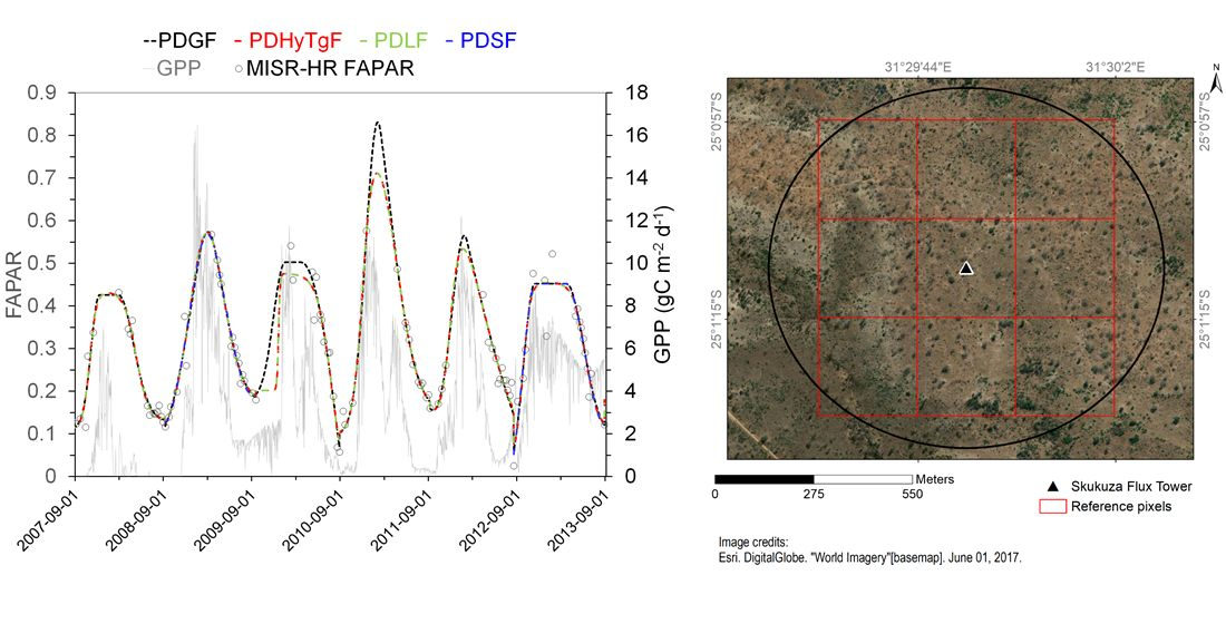
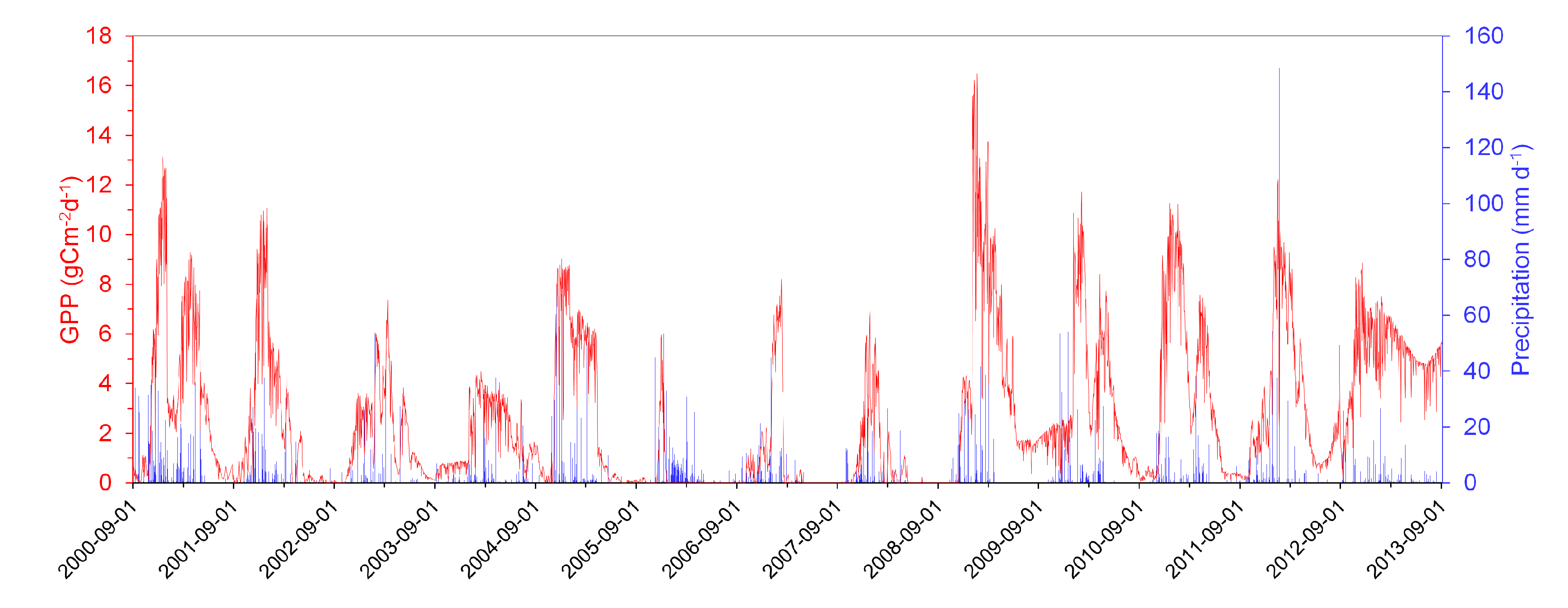
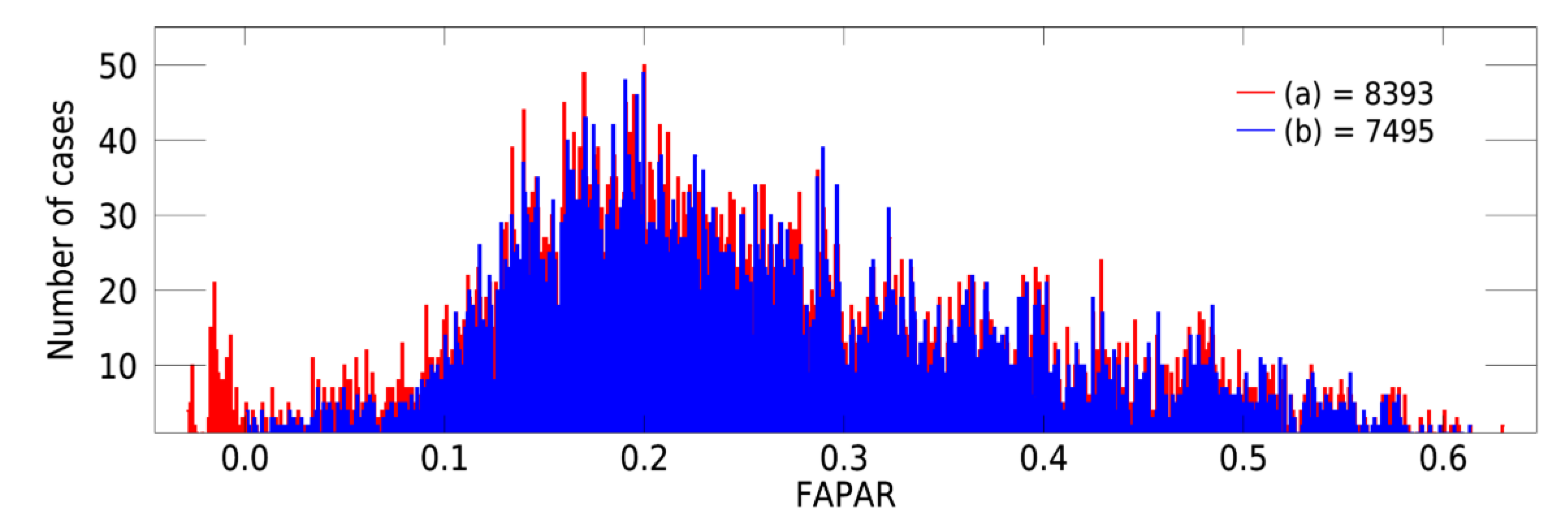
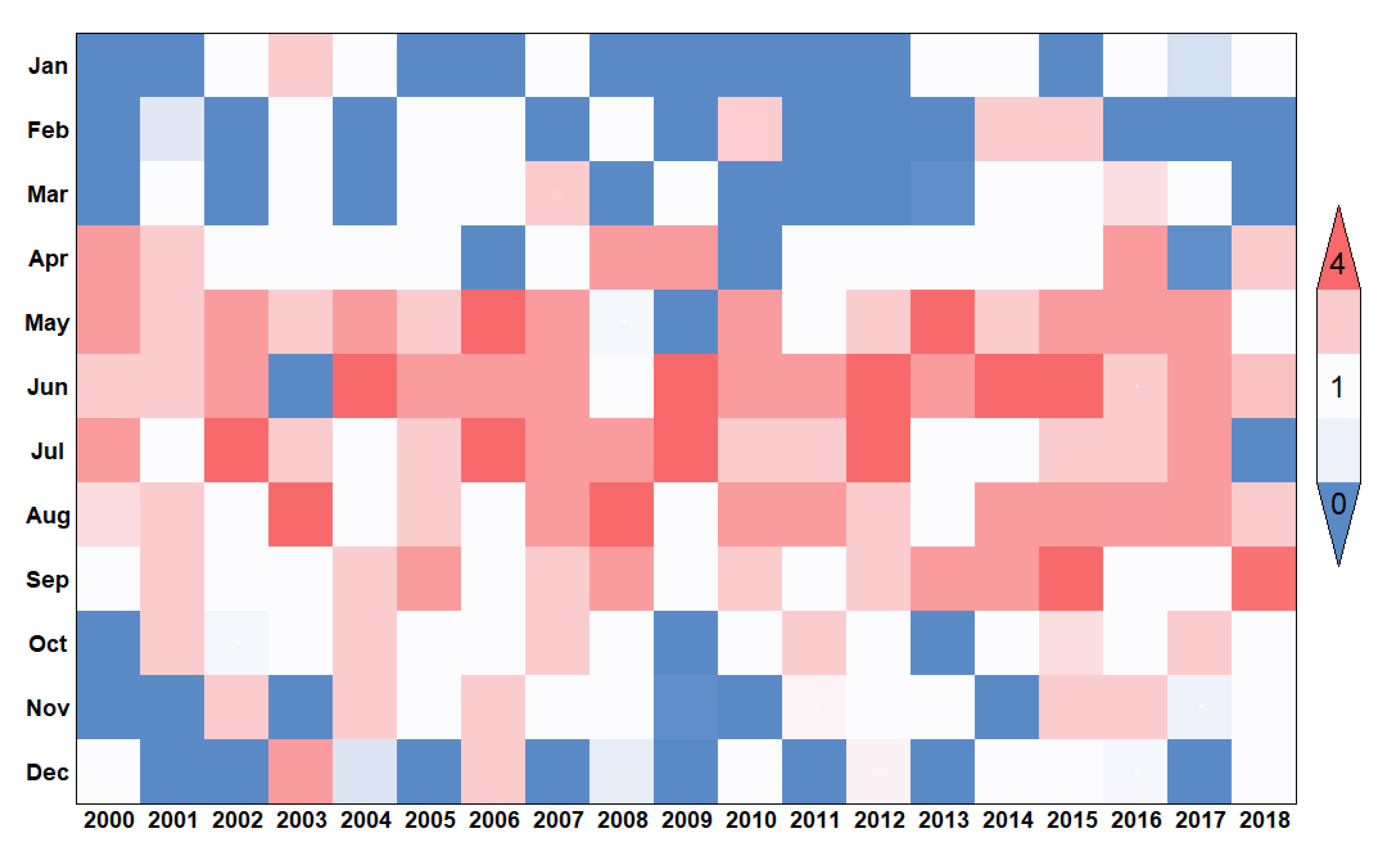
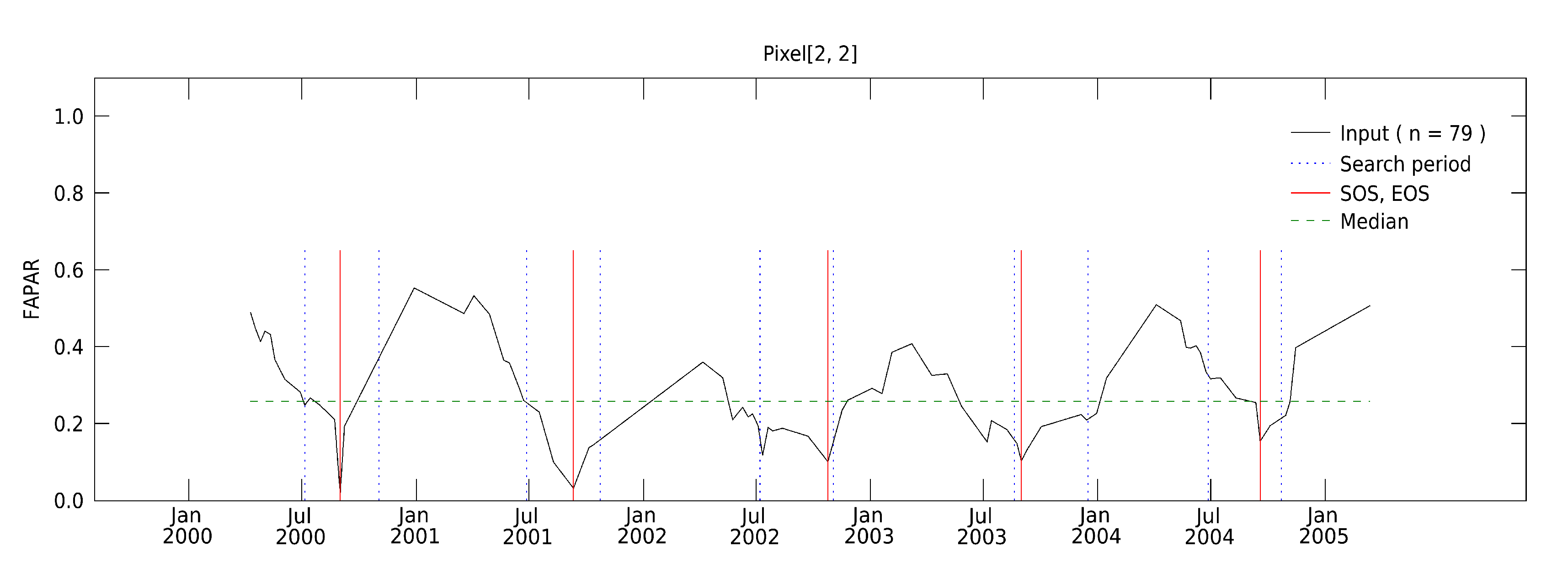
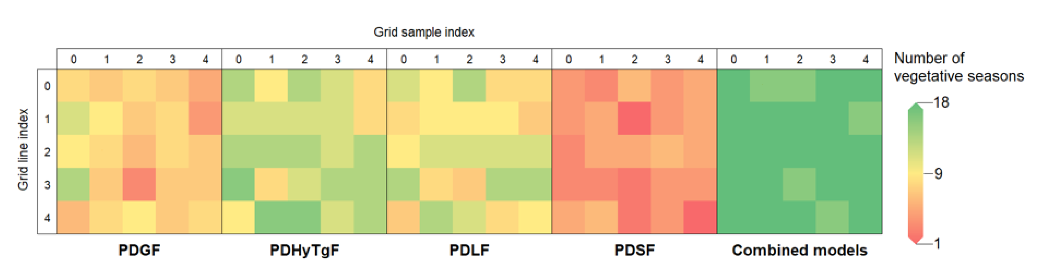
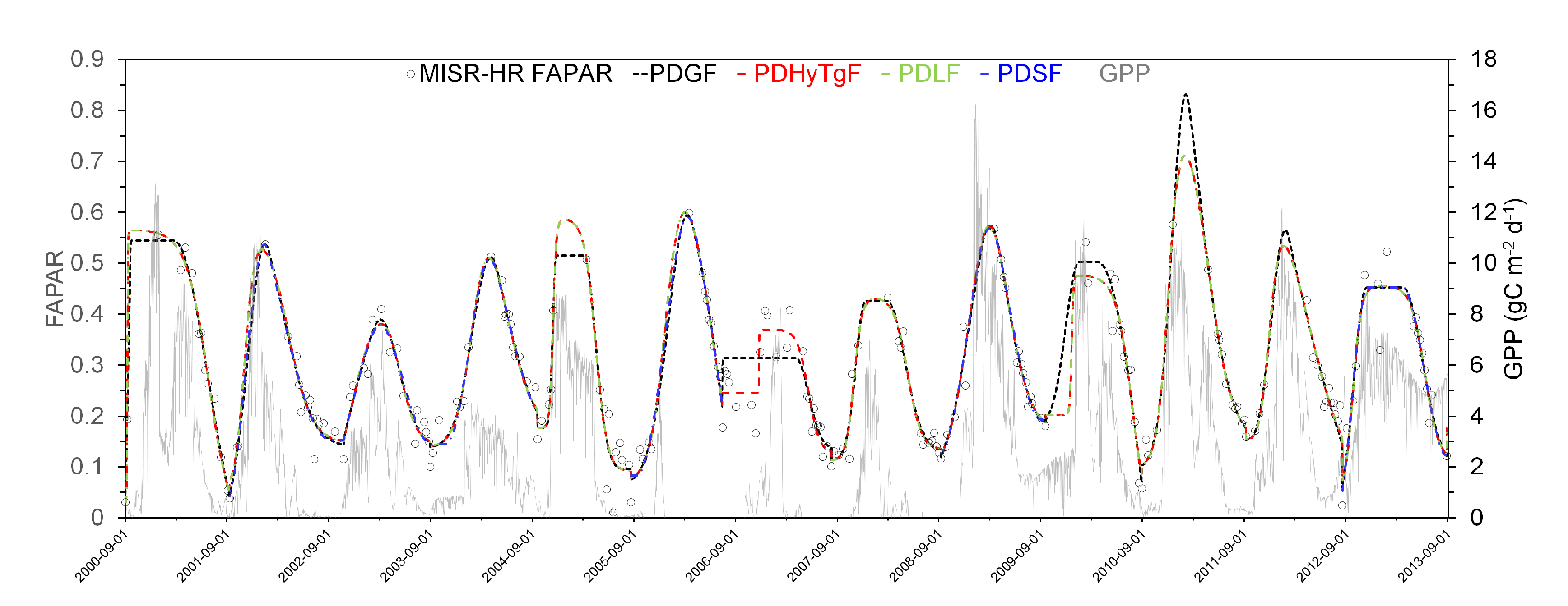
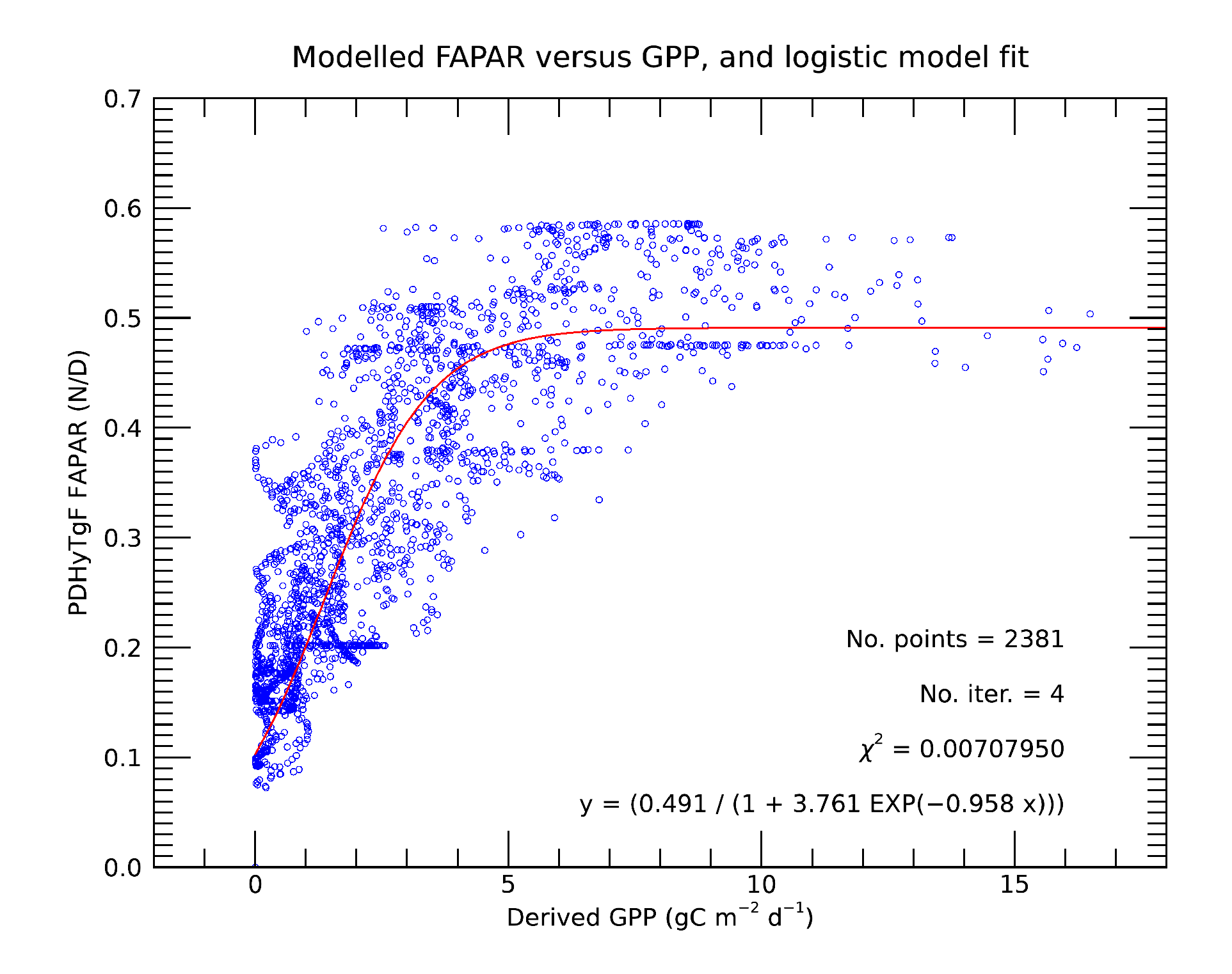
Table 1.
Relation between the largest allowable cost function value (Threshold), the number of data points identified as outliers, and the number of data points remaining available for further analysis in the time series of Figure 3.
Table 1.
Relation between the largest allowable cost function value (Threshold), the number of data points identified as outliers, and the number of data points remaining available for further analysis in the time series of Figure 3.
| Threshold | 0.1 | 0.08 | 0.06 | 0.04 |
|---|---|---|---|---|
| Outliers | 34 | 59 | 110 | 211 |
| Remaining | 303 | 278 | 227 | 126 |
Table 2.
Correlation coefficients (r) between the daily GPP and daily FAPAR estimates from the PDGF, PDHyTgF, PDLF, PDSF, and combined models for each vegetative season and for the area around the Skukuza flux tower. Entry A indicates that fewer than half of the expected GPP values were available, while entry B means that the model could not simulate the available FAPAR data.
| SOS/EOS | Vegetative Season | Season Length | GPP % | PDGFr | PDHyTgFr | PDLFr | PDSFr | Combinedr |
|---|---|---|---|---|---|---|---|---|
| 2000–08–31 | ||||||||
| 2001–09–10 | 1 | 375 | 99.2 | 0.56 | 0.52 | 0.52 | B | 0.56 |
| 2002–10–24 | 2 | 409 | 86.8 | 0.72 | 0.78 | 0.78 | 0.74 | 0.72 |
| 2003–08–31 | 3 | 311 | 100 | 0.71 | 0.70 | 0.70 | 0.70 | 0.71 |
| 2004–09–18 | 4 | 384 | 100 | 0.81 | 0.82 | 0.82 | 0.82 | 0.81 |
| 2005–08–20 | 5 | 336 | 94.6 | 0.92 | 0.93 | 0.93 | B | 0.93 |
| 2006–07–15 | 6 | 329 | 24.9 | A | A | A | A | A |
| 2007–08–10 | 7 | 391 | 41.4 | A | A | AB | AB | A |
| 2008–09–06 | 8 | 393 | 45.3 | A | A | A | AB | A |
| 2009–09–16 | 9 | 375 | 82.1 | 0.79 | 0.80 | 0.80 | 0.80 | 0.79 |
| 2010–08–27 | 10 | 345 | 100 | 0.69 | 0.72 | 0.72 | B | 0.69 |
| 2011–09–06 | 11 | 375 | 100 | 0.80 | 0.82 | 0.82 | B | 0.80 |
| 2012–09–01 | 12 | 361 | 100 | 0.82 | 0.80 | 0.80 | B | 0.82 |
| 2013–08–26 | 13 | 359 | 100 | 0.56 | 0.56 | 0.56 | 0.55 | 0.56 |
Table 3.
Correlations coefficients (r) between the integrated GPP and Cumulated FAPAR (CFAPAR) obtained by integrating the PDGF, PDHyTgF, PDLF, PDSG, and combined models during the indicated vegetative seasons. Computations were skipped whenever fewer than half of the expected GPP observations were available during the season, or when the correlation between the daily GPP and model values dropped below 0.70 in Table 2 (see text for details).
| SOS/EOS | Vegetative Season | Integrated GPP | CFAPAR | ||||
|---|---|---|---|---|---|---|---|
| PDGF | PDHyTgF | PDLF | PDSF | Combined | |||
| 2001–09–10 | |||||||
| 2002-10-24 | 2 | 815.25 | 117.72 | 122.26 | 122.26 | 118.50 | 117.72 |
| 2003–08–31 | 3 | 656.65 | 84.19 | 84.14 | 84.14 | 84.40 | 84.19 |
| 2004–09–18 | 4 | 682.33 | 119.50 | 119.91 | 119.91 | 119.24 | 119.50 |
| 2005–08–20 | 5 | 1043.88 | 105.95 | 111.70 | 111.70 | 111.70 | |
| 2009–09–16 | 9 | 1522.03 | 130.12 | 130.87 | 130.87 | 130.44 | 130.12 |
| 2010–08–27 | 10 | 1185.21 | 129.29 | 117.07 | 117.07 | 129.29 | |
| 2011–09–06 | 11 | 1314.19 | 155.09 | 148.36 | 148.36 | 155.09 | |
| 2012–09–01 | 12 | 1178.08 | 116.34 | 115.56 | 115.56 | 116.34 | |
| r | 0.65 | 0.62 | 0.62 | 0.65 | 0.65 | ||
| p-value | 0.35 | 0.38 | 0.38 | 0.35 | 0.35 | ||
Table 4.
Number and proportion of successful model inversions.
| Successes | PDGF | PDHyTgF | PDLF | PDSF |
|---|---|---|---|---|
| Number | 309 | 382 | 355 | 224 |
| Proportion (%) | 68.6 | 84.8 | 78.8 | 49.7 |
Table 5.
Number of iterations required, for successful (s) and unsuccessful (u) model inversions.
| Iterations | PDGF | PDHyTgF | PDLF | PDSF | ||||
|---|---|---|---|---|---|---|---|---|
| Cases | s | u | s | u | s | u | s | u |
| Minimum | 2 | 1 | 1 | 1 | 1 | 1 | 2 | 1 |
| 25th percentile | 7 | 1 | 8 | 2 | 8 | 1 | 7 | 1 |
| Median | 10 | 2 | 12 | 2 | 12 | 3 | 9 | 2 |
| Mean | 20.8 | 3 | 18.6 | 7.2 | 18.7 | 7.2 | 10.8 | 4 |
| 25th percentile | 14 | 3 | 19 | 4 | 19.5 | 4 | 11 | 3 |
| Maximum | 71 | 8 | 53 | 27 | 53 | 27 | 25 | 13 |
Table 6.
Execution time, relative to the fastest case (successful PDLF model inversion in 0.00299978 second), for successful (s) and unsuccessful (u) model inversions.
Table 6.
Execution time, relative to the fastest case (successful PDLF model inversion in 0.00299978 second), for successful (s) and unsuccessful (u) model inversions.
| Iterations | PDGF | PDHyTgF | PDLF | PDSF | ||||
|---|---|---|---|---|---|---|---|---|
| Cases | s | u | s | u | s | u | s | u |
| Minimum | 1.00008 | 1.00008 | 1.00008 | 1.33341 | 1.00000 | 1.00008 | 1.00008 | 1.00008 |
| 25th percentile | 1.66675 | 1.66675 | 1.66683 | 1.66675 | 1.66675 | 1.66675 | 1.66683 | 1.33341 |
| Median | 2.00008 | 2.00008 | 2.00016 | 2.00016 | 2.00016 | 1.66683 | 2.00016 | 1.66683 |
| Mean | 2.26680 | 2.53349 | 2.66686 | 2.13346 | 2.26680 | 2.06678 | 2.46685 | 1.93348 |
| 75th percentile | 2.00016 | 2.33349 | 2.33357 | 2.33349 | 2.33349 | 2.00016 | 2.33349 | 2.00016 |
| Maximum | 4.66708 | 5.66708 | 6.33383 | 3.33357 | 4.33365 | 4.00023 | 5.33372 | 3.66700 |
Table 7.
Average value at the end of the model inversion step.
| PDGF | PDHyTgF | PDLF | PDSF |
|---|---|---|---|
| 0.022 | 0.020 | 0.018 | 0.015 |
Publisher’s Note: MDPI stays neutral with regard to jurisdictional claims in published maps and institutional affiliations. |
© 2020 by the authors. Licensee MDPI, Basel, Switzerland. This article is an open access article distributed under the terms and conditions of the Creative Commons Attribution (CC BY) license (http://creativecommons.org/licenses/by/4.0/).
Share and Cite
MDPI and ACS Style
De Lemos, H.; Verstraete, M.M.; Scholes, M. Parametric Models to Characterize the Phenology of the Lowveld Savanna at Skukuza, South Africa. Remote Sens. 2020, 12, 3927. https://0-doi-org.brum.beds.ac.uk/10.3390/rs12233927
AMA Style
De Lemos H, Verstraete MM, Scholes M. Parametric Models to Characterize the Phenology of the Lowveld Savanna at Skukuza, South Africa. Remote Sensing. 2020; 12(23):3927. https://0-doi-org.brum.beds.ac.uk/10.3390/rs12233927
Chicago/Turabian StyleDe Lemos, Hugo, Michel M. Verstraete, and Mary Scholes. 2020. "Parametric Models to Characterize the Phenology of the Lowveld Savanna at Skukuza, South Africa" Remote Sensing 12, no. 23: 3927. https://0-doi-org.brum.beds.ac.uk/10.3390/rs12233927
Note that from the first issue of 2016, this journal uses article numbers instead of page numbers. See further details here.