Change Detection within Remotely Sensed Satellite Image Time Series via Spectral Analysis


1
Faculty of Science, University of Calgary, 2500 University Drive NW, Calgary, AB T2N 1N4, Canada
2
Faculty of Management, University of Lethbridge, 4401 University Drive W, Lethbridge, AB T1K 3M4, Canada
*
Author to whom correspondence should be addressed.
Remote Sens. 2020, 12(23), 4001; https://0-doi-org.brum.beds.ac.uk/10.3390/rs12234001
Submission received: 15 October 2020
/
Revised: 28 November 2020
/
Accepted: 3 December 2020
/
Published: 7 December 2020
(This article belongs to the Section Remote Sensing in Agriculture and Vegetation)
Abstract
:Jump or break detection within a non-stationary time series is a crucial and challenging problem in a broad range of applications including environmental monitoring. Remotely sensed time series are not only non-stationary and unequally spaced (irregularly sampled) but also noisy due to atmospheric effects, such as clouds, haze, and smoke. To address this challenge, a robust method of jump detection is proposed based on the Anti-Leakage Least-Squares Spectral Analysis (ALLSSA) along with an appropriate temporal segmentation. This method, namely, Jumps Upon Spectrum and Trend (JUST), can simultaneously search for trends and statistically significant spectral components of each time series segment to identify the potential jumps by considering appropriate weights associated with the time series. JUST is successfully applied to simulated vegetation time series with varying jump location and magnitude, the number of observations, seasonal component, and noises. Using a collection of simulated and real-world vegetation time series in southeastern Australia, it is shown that JUST performs better than Breaks For Additive Seasonal and Trend (BFAST) in identifying jumps within the trend component of time series with various types. Furthermore, JUST is applied to Landsat 8 composites for a forested region in California, U.S., to show its potential in characterizing spatial and temporal changes in a forested landscape. Therefore, JUST is recommended as a robust and alternative change detection method which can consider the observational uncertainties and does not require any interpolations and/or gap fillings.
Keywords:
EVI; jump detection; Landsat 8; Least-Squares estimation; NDVI; spectral analysis; Terra; time series; trend analysis
1. Introduction
Monitoring land cover changes using remote sensing satellite imagery has been well-established observationally and theoretically over the past few decades. Detecting changes within a remotely sensed time series and identifying their driving mechanisms can help policymakers, natural resource managers, and scientists to address many issues facing the planet, such as carbon budgets, global climate change, drought, and wildfires [1,2,3,4].
Remotely sensed time series usually contain trend and seasonal components, where the trend component represents variations of low frequency and the seasonal component is part of the variations representing intra-annual fluctuations that are more or less stable year after year [5,6]. Typically, changes occurring in the trend component are due to disturbances, including fires, deforestation, urbanization, insect attack, and flood, whereas, changes in the seasonal component are usually driven by the influence of temperature and rainfall on plant phenology [7,8].
Vegetation dynamics are often monitored at different spatial and temporal scales through vegetation index time series obtained from multi-spectral sensors onboard various Earth observation satellite systems, such as Terra, Landsat, Sentinel, and RapidEye. Two widely used spectral indices are Normalized Difference Vegetation Index (NDVI) [9] and Enhanced Vegetation Index (EVI) [10]. Once the topographic effects are removed via certain techniques, EVI (with respect to NDVI) can reduce the adverse effects of environmental factors, such as atmospheric conditions and soil background [11]. In fact, EVI can be considered as an improved NDVI because of its non-saturation property in high biomass regions and its ability to attenuate background and atmospheric noises.
Satellite images are not always available, and so most satellite image time series are unequally spaced (irregularly sampled over time with possibly large gaps). Popular time series analysis methods, such as the Fourier and wavelet transforms (e.g., [12,13,14]) require equally spaced time series, and thus many researchers strive to apply some interpolation techniques to make the time series equally spaced so that they can use these methods. However, data pre-processing, such as interpolation, may perform poorly and introduce undesirable biases in the results [15,16]. On the other hand, current change detection algorithms rely heavily on an effective cloud masking procedure (e.g., [17,18,19]) to remove contaminated pixels (e.g., cloudy, hazy, smoky) in advance of the analysis. Thus, depending on the robustness of a cloud detection method and weather conditions, many pixels may be ignored, and thus many researchers apply some questionable methods to fill in the gaps and make the time series equally spaced [7,20]. A robust cloud detection method should provide the degree or level of uncertainties for possibly contaminated pixels, and a robust change detection method must consider these uncertainties instead of simply removing such pixels that can create large data gaps in the time series. One may define appropriate weights associated with the time series values to account for such uncertainties, making time series unequally weighted [21,22].
Change detection within remotely sensed time series is a challenging problem because such time series are often unequally spaced and have trend, seasonal, and other components. Many methods have been proposed for detecting changes within non-stationary time series, such as the Breaks For Additive Seasonal and Trend (BFAST) [7,8], Continuous Change Detection and Classification (CCDC) [23], Seasonal-Trend decomposition procedure based on Loess (STL) [24,25], Detecting Breakpoints and Estimating Segments in Trend (DBEST) [26], and others [27,28,29]. However, almost all of these methods are limited to equally (regularly) spaced time series and do not consider the observational uncertainties in the time series values that can significantly improve the estimation of breakpoints (jump locations), trend and seasonal components.
The Least-Squares Wavelet Analysis (LSWA) is a novel technique of time series analysis based on the Least-Squares principle and an appropriate segmentation [30]. LSWA decomposes a time series into the time-frequency domain which enables the detection of periodic and aperiodic signals. The Anti-Leakage Least-Squares Spectral Analysis (ALLSSA) is an iterative algorithm that can accurately estimate the trend and seasonal components [31]. ALLSSA and LSWA are the main tools in the Least-Squares Wavelet (LSWAVE) software [32,33]. They are successfully applied to estimate the trend and seasonal components in the NDVI and EVI time series [21,34]. One of the main advantages of ALLSSA and LSWA is their ability to analyze unequally spaced and weighted time series as they are given without any need for pre-processing including interpolations and gap-fillings. The LSWAVE software currently requires the user to manually enter the time instances when datum shifts (offsets) occur for a more accurate estimation of the seasonal component. Herein, an ALLSSA based method is proposed to estimate such time instances in a more general case.
Therefore, the goal of this research is to develop a robust change detection method for time series which involves the detection and characterization of Jumps Upon Spectrum and Trend (JUST). The main objectives of this research are:
- The detection of jumps (sudden changes) in the trend component of an unequally spaced time series;
- Accounting for uncertainties in the time series values (observational uncertainties) to improve the estimation of trend and seasonal components, and jump locations; and
- The characterization of the gradual and sudden changes in the ecosystem by estimating the jump direction and magnitude.
The ALLSSA season-trend model, the core of JUST proposed herein, was used for selecting a stable history period for near-real-time monitoring [21]. In this article, the focus is detecting disturbances within the historical time series like BFAST [7,8]. JUST segments the entire historical time series and applies ALLSSA to each segment to find potential jumps. JUST then finds an optimal set of jump locations for the entire time series and finally divides the time series into trend, seasonal, and remainder components like BFAST. JUST is assessed by simulating EVI time series and changing the number of observations, seasonality, noise level, and by adding sudden changes with different magnitudes. JUST is also compared with BFAST using simulated time series with various types and two NDVI time series for a forested region in southeastern Australia. Another reason for choosing BFAST for the comparison herein is that BFAST is a popular change detection method whose advantages and weaknesses are shown by many researchers [35,36,37,38,39], and herein it is also aimed to show the source of some of its weaknesses. The potential of JUST for jump detection and classification is also shown on a collection of Landsat 8 images covering a forested region in the northeast part of Santa Rosa in California, U.S., where BFAST cannot be directly applied as the time series are (inherently) unequally spaced, and BFAST does not consider the observational uncertainties.
2. Materials and Methods
2.1. Study Regions
The top right panel of Figure 1 illustrates two different study regions chosen herein to test and validate the performance of JUST in detecting and classifying changes within real-world vegetation time series. The first region is a forested area (Pinus radiata plantation) in southeastern Australia, selected herein to compare BFAST with JUST [8]. The second study region is mainly a forested region (≈1600 km) located in the northeast part of Santa Rosa, the main city in California’s famous Wine Country. The second region is covered by a mixture of shrubs and trees, such as oak, madrone, alder, and redwood [40,41]. The ground reference areas, displayed as polygons with semi-transparent fill color toward the north and east of Santa Rosa in the magnified section of Figure 1, are mainly impacted by the massive wildfires in October 2017, known as Tubbs Fire, Nuns Fire, and Atlas Fire [42]. The polygon shapefiles for the burned areas within the second study region, used for validation herein, are obtained from the Monitoring Trends in Burn Severity, conducted through a partnership between the U.S. Geological Survey National Center for Earth Resources Observation and Science and Forest Service Remote Sensing Applications Center, the U.S. Department of Agriculture [43]. Another reason for selecting the second study region is the availability of Landsat 8 satellite imagery every seven and nine days (because of the spatial overlapping of satellite images in higher latitudes), making the image time series (inherently) unequally spaced, see below and [21,44] for more details.
2.2. Data Sets and Pre-Processing
Two NDVI time series from 2000 to 2009 are used for the first study region to compare BFAST with JUST. The 16-day Moderate Resolution Imaging Spectroradiometer (MODIS) NDVI composites (250 m spatial resolution) are used to obtain these two time series which are the same as the ones shown in the middle and bottom panels of Figure 8 in [8], downloaded from [45]. The binary MODIS Quality Assurance flags are used to choose the cloud-free data with optimal quality. The NDVI time series corresponding to the bottom panel of Figure 8 in [8] has several missing values, replaced by linear interpolation between neighboring values within the time series before applying BFAST [8,45]. However, no interpolation technique is required when applying JUST.
For the second study region, Landsat 8 surface reflectance data products from the U.S. Geological Survey (USGS) with 30 m spatial resolution are used [47]. The Landsat 8 satellite is in a near-polar, sun-synchronous, circular orbit with 705 km altitude and has a 16-day repeat cycle [48]. The Landsat orbits are poleward convergent, and thus Landsat 8 sensor can acquire more frequent scene coverage at higher latitudes [49]. The amount of Landsat data in the U.S. Landsat archive is not constant temporally and spatially among Landsat sensors due to various factors, such as sensor health, and the capability of data reception and acquisition [48,49,50]. According to the product guide for the Landsat 8 surface reflectance code, the calibration parameters from the metadata files associated with the Landsat 8 data are used to generate Top Of Atmosphere (TOA) reflectance and TOA brightness temperature. Then an atmospheric correction procedure is applied to Landsat 8 TOA reflectance data, using additional input data, such as water vapor, ozone, and aerosol optical thickness, as well as a digital elevation derived model to generate the surface reflectance data products.
The surface reflectance bands 2 (Blue), 4 (Red), and 5 (Near Infrared) are used to calculate EVI defined as follows
where , , and signify the spectral reflectance measurements acquired in the Near Infrared, Red, and Blue regions, respectively. Coefficients G, L, , and are the gain factor, canopy background adjustment, and aerosol resistance terms, respectively [10]. Herein, the adopted coefficients , , , and for the Landsat 8 imagery are used [51]. The scale factor is multiplied by each band value to convert their values to floating point values from 0.0 to 1.0 before calculating EVI. This scale multiplication is not necessary for NDVI because NDVI defined by
with the value range from to 1, does not have the adjustment factor L [11,34,52]. The value range for EVI is usually from to 1 (may exceed) and varies between and for healthy vegetation [52].
2.3. Weighted Vegetation Time Series
A per-pixel vegetation time series is obtained from a set of spatially aligned pixels in the vegetation images, also referred to as vegetation time series [21]. Figure 2 demonstrates the process of obtaining an EVI time series from a set of spatially aligned pixels (shown in solid colors). The Pixel Quality Assessment (PQA) band obtained for each Landsat 8 satellite image is used to define the weights. According to the product guide for Landsat 8, if a pixel value in the PQA band is 322, 386, 834, 898, or 1346, then the pixel is clear, otherwise, there is a high chance that the pixel is contaminated with clouds, cloud shadows, water, snow, ice, smoke, or haze. The following technique shows how one may obtain a weighted vegetation time series using the PQA band.
The key point here is to assign lower weights to the observations with higher uncertainties, and vice versa. For a given Landsat 8 EVI image, first count the number of pixels for each spatial window of size nine whose PQA band values are not equal to 322, 386, 834, 898, or 1346 and denote it by . To account more for the observational uncertainty corresponding to the pixel located at the window center, add one unit to if that pixel is contaminated, so . If , then there is a high chance that the pixel in the center of the spatial window is contaminated, and so one may mask out that pixel (ignore the observation). Otherwise, assign an appropriate weight to each pixel located at the window center, herein defined by and multiplied by 100 to express it as percentage. Therefore, for all spatially aligned windows with the same region coverage, a weighted vegetation time series will be obtained for the spatially aligned pixels located at centers of the spatial windows, see the shaded gray and solid pixels in Figure 2 used to define weights for the solid pixels. Continuing this process for all the spatially aligned pixels located at the centers of the spatially aligned windows, a set of weighted vegetation time series will be obtained covering a region of interest (the second study region herein). For each pixel, considering the uncertainties in its neighboring pixels can reduce the noise effect of the pixel during the season-trend analysis because it is possible that the PQA band incorrectly states that the pixel is clear (cloud-free, etc.) while the PQA band shows some of the neighboring pixels are in fact contaminated. Choosing larger sizes for the spatial window (e.g., 25 pixels) may also provide a more reliable weight for the pixel in the center of the spatial window. The weighting procedure presented here could be applied to image time series prior to any change detection method. Therefore, this is an option for a generally improved pre-processing of optical satellite data.
2.4. Jumps Upon Spectrum and Trend (JUST)
This section focuses on analyzing a time series that can be a weighted vegetation time series. JUST is established by simultaneous estimation of spectrum and trend for a given time series with an associated covariance matrix whose inverse, denoted by (weight matrix), can be used to control the effect of noisy measurements [30]. Please note that the relative weights play a significant role for improving the estimation of trend and seasonal components, but the proposed method is not sensitive to any covariance factor [53]. In the next section, the weight matrix is a diagonal matrix whose diagonal entries are obtained from the observational uncertainties and is treated as a vector for the sake of computational efficiency. The seasonal component of the time series may not be stable over time, i.e., its frequencies and amplitudes may change over time, and so performing the spectral analysis on the entire time series can potentially reduce the accuracy of estimating the trend and seasonal components [30]. To detect jumps, a temporal segmentation technique is proposed to account for changes within the trend and seasonal components. A sequential approach is then performed that scans each time series segment using ALLSSA to determine statistically at which location there exists a significant jump in the segment.
For a better understanding of the segmentation of the time series, the term window (temporal window) is used. In this terminology, a window contains a time series segment with its associated statistical weights as well as the constituents of known forms (e.g., linear trend) and sinusoidal functions being fitted to the segment [30]. The window size R is defined as the number of observations within the window or simply the segment size. However, the window length is the time difference between the last and the first observations within the window [30]. For an unequally spaced time series, a translating window with a fixed size rather than a fixed length may contain additional observations from the neighboring seasons which may allow better estimation of trend and seasonal components, a useful approach when there are few observations available within a particular season [54]. Please note that the window size selected herein is fixed during translation by observations over time, and it is independent of frequency, a special case of LSWA when the window size parameter is zero [30].
For each segment of size R within the translating window, ALLSSA can be set up to find an optimal piece-wise linear function with two pieces along with a set of estimated sinusoidal functions (the sequential approach). In other words, the constituents of known forms in ALLSSA may be selected as the linear functions with two pieces whose intercepts and slopes will be simultaneously estimated with the sinusoidal functions. Therefore, sequentially two linear pieces will be selected that along with the estimated sinusoids minimize the weighted L2 norm of the residual segment, where the residual segment is the original segment minus the estimated linear trend with two pieces and the estimated sinusoids. In ALLSSA, for a given linear trend with two pieces as the constituents of known forms, the frequencies and amplitudes of the sinusoidal functions will be estimated simultaneously with the intercepts and slopes of the two linear pieces until there is no more statistically significant peak in the spectrum at a certain confidence level (usually selected at which corresponds to the significance level ).
Now, let and be the estimated slopes and and be the estimated intercepts of the two linear pieces for the segment, respectively. These estimated coefficients can be used to derive the direction and magnitude of the potential jump respectively as
where the hat symbol stands for estimation, and is the time of the potential jump determined by the sequential approach. Please note that JUST can also detect as the time when a jump in trend occurs even if because the intercepts and slopes of the two linear trends can be different ( but still making the magnitude equal to zero (the word “jump” is used loosely in this case).
Figure 3a demonstrates three time series such that each has a jump at (the ninth observation). The time series whose observations are shown by the blue circles has a weak jump at with a small negative direction and a small positive magnitude. For example, a very small and negligible part of an arid region, corresponding to a per-pixel NDVI time series, starts growing plants around the jump location. One may disregard this jump by applying certain thresholds (e.g., and , where is the absolute value). The time series, shown by red diamonds, has a jump with . For example, in real-world applications, a jump with a negative magnitude may have been created by harvesting, wildfire, insect attack, etc. The time series, shown by green squares, has a jump with positive direction and zero magnitude, e.g., it may have been created indirectly by irrigation after a gradual drought.
JUST evaluates a determined jump location (breakpoint) by its occurrence that is the number of times that is determined as a jump location within all the windows containing . When there are several identical or close enough jump locations, each detected within a window, JUST selects the one that has the maximum occurrence, then the one whose time index ℓ is closer to the time index of its corresponding window location [30]. The latter is because the selected has data support from both sides of the window, making the magnitude and direction of the jump more accurate [30,31]. Certain thresholds for the direction and magnitude of a jump may be applied at this point to ignore weak changes and to reduce false-positive rates in real-world applications.
Given the jump locations, ALLSSA may optionally be applied to a new set of segments to estimate the trend and seasonal components within each segment. A weighted moving average method, whose weights are obtained from a symmetric Gaussian function [30], may then be applied to estimate the trend and seasonal components of the entire time series. Alternatively, given the jump locations, the LSWAVE software may be implemented to study seasonal changes in the time-frequency domain [32].
To understand the JUST algorithm better, an NDVI time series along with two windows are illustrated in Figure 3b. The red window translates to the green window by observations (the windowing or segmentation approach). Within each window, the sequential approach is performed which finds a potential jump in the segment, see the red and green arrows pointing to the jumps detected within the red and green windows, respectively. Since the two detected jump locations are close to each other, JUST selects the point in the segment within the green window (see the green arrow) because it has more observations on its right hand side within the green window to support a more reliable simultaneous estimation of trend and seasonal components. Having the list of all detected jump locations within translating windows is useful as it may also reveal the potential outliers. For example, the observation shown by the red arrow in Figure 3b, may be an outlier due to the presence of atmospheric or background noise that could not be detected from a cloud masking method, neither an appropriate weight could be assigned to this observation to mitigate its effect [21,55]. Please note that within each window, ALLSSA estimates a separate set of sinusoidal functions that can change as the window translates to account for the phenological changes [7,8,56]. Figure 4 shows the flowchart of JUST for the sake of completeness.
The Ordinary Least-Squares (OLS) estimation simply fits the constituents of known forms, such as trends and sinusoids of known frequencies to the time series to estimate their coefficients [22]. For each time series segment, the OLS-based method proposed herein (the simple case of JUST) finds an optimal piece-wise linear function with two pieces along with sinusoidal functions of fixed cyclic frequencies ( cycles per year) like in BFAST. The flowchart of the OLS-based method for a given time series is the same as the one shown in Figure 4 but instead of applying ALLSSA, OLS is applied to estimate the trend and sinusoids of fixed cyclic frequencies ( cycles per year) for each segment. The OLS estimation not only may increase the false-positive rate for change detection but it may also cause the over/under-fitting problem [21,57]. Unlike the OLS-based method, JUST searches each segment to find statistically significant spectral peaks without any assumptions on the existence of seasonal component and its frequencies. JUST simultaneously estimates the trend and statistically significant seasonal components within each segment, introducing a robust change detection method.
To validate the sequential approach and also to seek an effective window size for the segmentation approach, in Section 3.1.1 and Section 3.1.2, the results of jump detection methods using two window sizes and are compared, where M is an average sampling rate. For an unequally spaced time series, the sampling rate cannot be a fixed number [58], and so an average sampling rate may be computed as , where n is the number of observations, is the start time, and is the end time, e.g., observations per year, where and . Both window sizes can account for inter-annual variations caused by several factors, such as climate change, land management or land degradation [7,59]. It is shown that selecting window size performs better in identifying true jumps within time series with poorer signal-to-noise ratio than , however, can be a better choice for less noisy time series whose components have more variability of amplitude and frequency over time. Please note that noise in this context refers to components other than trend and seasonal, such as random noise from cloud contamination, and other high-frequency signatures. For the automation purposes in environmental applications, and are recommended. This selection is capable of detecting jumps occurred approximately one year apart and is robust in capturing inter-annual and seasonal variations within satellite image time series. The main inputs and outputs of the JUST code are listed in Table 1.
2.5. Breaks for Additive Seasonal and Trend (BFAST)
This section briefly describes BFAST due to its similarities to JUST and the numerical comparisons made in the next section. BFAST is an iterative algorithm that decomposes a time series into trend, seasonal, and remainder components [7]. The trend component between any two consecutive jump locations is assumed to be linear and the seasonal component is estimated by summing the cosine and sine (sinusoidal) functions of fixed frequencies (e.g., 1, 2, 3 cycles per year). The OLS residual segment is obtained by subtracting the estimated trend and/or sinusoidal functions of fixed frequencies via the Least-Squares fit from the segment [22,60].
The iterative process starts by estimating the seasonal component using a standard season-trend decomposition. The Ordinary Least-Squares Residuals-Based Moving Sum (OLS-MOSUM) is performed to verify whether there are any jumps occurring in the trend component. If the OLS-MOSUM test shows breakpoints are occurring in the trend component, then their numbers and locations are estimated by the Least-Squares from the seasonally adjusted data, i.e., from the time series minus the estimated seasonal component. Given the breakpoints, the intercepts and slopes of the linear trends are estimated using a robust regression based on M-estimation [61]. If the OLS-MOSUM test shows breakpoints are occurring in the seasonal component, then their numbers and locations are estimated by the Least-Squares from the detrended data, i.e., from the time series minus the estimated trend component. The amplitudes of the sinusoidal functions are estimated using a robust regression based on M-estimation to estimate the seasonal component. This process is iterated until the numbers and positions of the breakpoints no longer change.
2.6. Validation through Descriptive Statistics
Suppose that there are K time series where each time series has a known jump at a specific location, and a change detection method is set to detect a maximum of one jump in each time series. The following statistical measures are used for validation in the next section:
- Jump error for the K time series: the number of incorrectly detected jump locations divided by K, i.e., normalized.
- Root Mean Square Error (RMSE) for the jump magnitude when the jump location is correctly detected:where m is the number of correctly detected jump locations (), and are the true and estimated magnitudes of a correctly detected jump, respectively, see Equation (4).
- Mean Normalized Residual Norm (MNRN): compute the Normalized Residual Norm (NRN) for each of the K time series, then find their average. For a given time series, NRN is defined as the weighted L2 norm of estimated residual series divided by the weighted L2 norm of the original series. More precisely:where f is a time series with its associated weights w (if available), n is the number of observations, and r is the residual series obtained after subtracting the estimated trend and seasonal components from f.
3. Results and Discussion
JUST can be applied to any non-stationary time series, and it is not limited to satellite image time series. In JUST, a time series can be equally or unequally spaced and does not require any interpolations or gap fillings, neither it manipulates the observations (i.e., JUST does not repair the data and analyzes them as they are provided). JUST determines whether there are any statistically significant components in the time series, and it accurately estimates the components by considering the observational uncertainties. In this section, JUST and its simple case (the OLS-based method) are validated using simulated and real-world vegetation time series with varying trend and seasonal components, and noises. Furthermore, JUST is compared with BFAST using both simulated and real-world vegetation time series.
3.1. Simulation Experiment
Simulation of satellite image time series is very challenging due to its immense dependence on various factors, such as vegetation phenology, inter-annual climate variations, sensor conditions (e.g., viewing angle), and signal contamination (e.g., clouds) [20]. Therefore, if there are any periodic signals in the time series, their cyclic frequencies can be any real numbers, and so it is necessary to estimate them accurately using statistical inference in order to detect jumps rigorously. Below, the advantages of JUST over the OLS-based method and BFAST are shown by simulating noisy time series with unknown seasonality, i.e., when the seasonal component of the time series cannot be well estimated by the sum of sinusoidal functions whose cyclic frequencies are integers.
3.1.1. Simulation of Time Series with Unknown Seasonality
To show the advantages of JUST over the OLS-based method, an EVI time series is simulated by summing a seasonal component S:
and a piece-wise liner trend function with two pieces:
To represent cloud contamination that may remain after atmospheric and cloud masking procedures, a noise component is added using a random number generator following a normal distribution with mean zero and standard deviation [7]. Thus, , . Hereafter, the noise level is expressed as , which is approximately of the noise range to allow one to compare the noise level with magnitude.
Since in the Landsat 8 data example, the images are acquired every nine and seven days consecutively, in the simulated examples, the distribution of the are set up accordingly unless stated otherwise. In other words, follow the sequence of divided by . Note that JUST does not depend on the distribution of , and it can be directly applied to any equally or unequally spaced time series without the need for any interpolations.
For some given sets of amplitudes from 0 to , phases from 0 to , and cyclic frequencies from to 4 (), 1000 time series are generated for each noise level in , while randomly removing up to of observations from each time series and changing the jump location. The locations of true jumps in all the simulated time series are recorded to check them against the estimated ones (model sensitivity test). For each noise level, the OLS-based method and JUST are applied to the same 1000 time series to estimate the jump locations, magnitudes, and residual series. Therefore, for each noise level and for each change detection method, the jump error, RMSE, and MNRN for the 1000 time series are also computed, see Section 2.6 where and the weights w are not considered.
Figure 5 shows the results of analyzing the 1000 time series for each noise level when the parameters in Equations (7) and (8) are given by , , , , , , , and . Each panel in Figure 5 shows four different plots for each method, obtained for four different magnitudes listed in Table 2, in red, in pink, in green, and in blue, where . Comparing the two methods, the OLS-based (dashed lines) and JUST (solid lines), one can clearly observe that JUST performs much better than the OLS-based method in all aspects of jump error, RMSE, and MNRN.
Figure 5a shows that when the noise level is less than the magnitude, the jump error in JUST is less than . The jump error gradually increases when the noise level increases for each magnitude. On the other hand, the jump error in the OLS-based method decreases when the magnitude increases because the effect of the seasonal component decreases. The RMSE results shown in Figure 5b also indicates that accurate estimation of seasonal component in JUST significantly improves the estimation of magnitudes. RMSE in the OLS-based method decreases as the magnitude increases because increasing the magnitude mitigates the effect of seasonal component. Figure 5c shows how MNRN in JUST is less than MNRN in the OLS-based method, signifying that the accuracy of estimated trend and seasonal components using OLS is generally poorer than ALLSSA.
The same analyses with the same values for the parameters mentioned above are performed on a longer time series (a three-year period), and the results are illustrated in Figure 6. The results show that when the noise level is less than the magnitude, the jump error in JUST is less than . Comparing Figure 6 with Figure 5, one can clearly observe that the jump error and RMSE of magnitudes decrease significantly when three years of data are used. The increase in MNRN values using OLS for the three years case is mainly due to the additional errors coming from the additional observations. Therefore, when a time series has stable seasonal component over time and three years of data are used to estimate the jump locations and magnitudes, the results are more resistant to poorer signal-to-noise ratio. However, this conclusion is more valid when the components are almost stable over time, and the time series does not have multiple jumps within the specified time period.
JUST is also tested for other values of amplitudes, phases, frequencies, and trend coefficients, and similar results are obtained, but not shown here for brevity. When the seasonal component can be well estimated by sinusoidal functions whose cyclic frequencies are integers, the OLS-based method and JUST produced very similar results (e.g., when setting , , and ). However, in practice, the cyclic frequencies can be any real numbers.
To compare JUST with BFAST, since BFAST R-code [45] does not support unequally spaced time series, for each noise level, 1000 equally spaced time series are simulated for a three-year period (16-day, about 23 observations per year) with the same set of coefficients for the sinusoidal functions (except in Equation (7)) and with the trend coefficients listed in Table 3.
BFAST and JUST are applied to the same set of time series, and the jump detection results are shown in Table 4. As the results in this table show, JUST performed much better than BFAST in detecting the true jump and estimating its magnitude particularly when . The higher the magnitude gets, the closer the results of BFAST become to the ones in JUST because the seasonal component is less dominant at higher magnitudes. In fact, since BFAST is designed according to OLS-MOSUM with fixed frequencies [7], it cannot rigorously estimate the true seasonal component, causing significant biases into its model, and thus performs poorly in cases when the seasonal component is unknown (e.g., waves whose frequencies are any real numbers and can change over time). The jump error in BFAST appears to slightly decrease with noise for (with ) and . This is likely due to the accidental detection of jumps at higher noise levels as the unknown seasonal component possibly becomes less dominant. The jump error in BFAST increases with noise when as the effect of seasonal component reduces at higher magnitudes and the increased noise level decreases the accurate detection of jumps. However, the jump error in BFAST is significantly higher than JUST in this example.
3.1.2. Simulation of Time Series with Two Noises of the Same Type
To demonstrate another advantage of JUST, the performance of JUST is examined when considering the weights. To do so, in addition to , another noise component is added to the time series as described below. To show the possibility of the existence of other types of seasonal component in certain land covers, the following asymmetric Gaussian function G is used:
where A is the amplitude, is the position of the maximum with respect to the independent time variable t, and and are positive numbers that determine the width of the left and right hand sides, respectively [7]. Herein, only a case is shown when , and S is defined as
Let , , where is the absolute value and is given by Equation (8). The noise level for is set to to account for noise that may remain after the cloud masking and atmospheric correction procedures, see Figure 7. Since in forested and vegetated lands, the EVI values are positive, cloud contamination will typically decrease the EVI values, the reason why the absolute value of is subtracted from the simulated EVI time series [21]. For each noise level in , 1000 time series are generated while randomly removing up to of observations from each time series and changing the jump locations. The true jump locations are recorded to test the model sensitivity. Noise is defined after the cloud masking procedure that can be partially controlled by introducing appropriate weights, e.g., , , so that the noisier measurements get lower weights during the analysis [21,30].
JUST is applied with and without considering the weights to estimate the jump locations, magnitudes of change, and residual series. Figure 8 shows the results of JUST with (solid lines) and without (dashed lines) considering the weights for the four different magnitudes listed in Table 2. From Figure 8, one can clearly observe that considering the weights in JUST (weighted JUST) reduces the jump error, RMSE of magnitudes and MNRN, and the differences between the results of weighted and unweighted JUST increase gradually as the noise level increases.
To test how considering an additional year of data can alter these results, the seasonal component of the time series is simulated by
while other components have the same structures as before. Figure 9 shows the new results, signifying that using three years of data in this example can also decrease the jump error and RMSE of magnitudes significantly for noisy observations.
JUST has been successfully tested for some other values for A, , , , and trend coefficients, and similar results are obtained, not illustrated here. Generally, for time series with almost stable seasonality over time, using three years of data improves the accuracy of jump locations and magnitudes, and it is more resistant to the poorer signal-to-noise ratio (having higher true positive rate). This accuracy will improve when the weights associated with the time series values are also considered in JUST.
To compare BFAST with the unweighted JUST when the seasonal component is defined by Equation (11), for each noise level , 1000 equally spaced time series are simulated (16-day, for a three-year period) with the trend coefficients listed in Table 3. The results of both methods on the same set of time series are shown in Table 5. Comparing Table 4 and Table 5, the BFAST results are improved in this case because the asymmetric Gaussian components can be estimated better using the harmonic functions with fixed frequencies. However, JUST still performed better than BFAST in most cases.
3.1.3. A Simulated EVI Time Series with Multiple Jumps
To show how JUST can detect multiple jumps in the trend component of an inherently unequally spaced time series, an EVI time series is simulated that has one observation every nine and seven days since 2013 with missing values. The seasonal component of this time series is defined using Equation (7), where , , , , , , and . Two jumps are introduced in years 2016 and 2018 with magnitudes and (EVI), and directions and (EVI per year), respectively. The seasonal, trend, and noise ( noise level) components are added to generate the time series. Then the absolute value of noise ( noise level) is subtracted from half of randomly selected time series values, see Figure 10a. The JUST decomposition results are shown in Figure 10, signifying that the proposed approach can rigorously considers the weights to accurately detect the jump locations and estimate the trend and seasonal components without any need for interpolation.
As described earlier, noise is used to define the weights. As it can be seen in Figure 10b, half of the observations are associated with weights equal to 100 because they are assumed clean observations (cloud-free, etc.), although they are still contaminated by noise (the noise that often remains after the atmospheric correction and cloud detection procedures). The other half of observations are associated with weights less than 100 according to noise . In real-world applications, these weights may be defined from a cloud detection algorithm (see Section 2.3). Many researchers mask the noisy observations using a cloud score threshold (e.g., remove the observations whose corresponding cloud scores are greater than ). However, removing such observations may result in getting a very coarsely sampled time series. JUST has this feature to keep these observations, but instead it considers their uncertainties because these observations may still be clean and valid.
3.2. Detecting and Characterizing Jumps in the NDVI Time Series for the First Study Region
For the first NDVI time series shown in Figure 11, one can observe that JUST and BFAST with their default parameters have detected four jumps. JUST has accurately detected a jump corresponding to the harvesting operation activity in August 2004, however, BFAST detected a jump in September 2004. When the number of jump locations is set to two, BFAST detects a jump in October 2004 that is more than one month ahead of the harvesting period. Furthermore, in Figure 11c, BFAST shows an unusual seasonal anomaly in the early 2005 which disappears when the number of jump locations is set to two, signifying the model sensitivity to the input parameters. BFAST has detected another jump in December 2005 with a small magnitude but large direction while JUST has detected a jump in May 2006. Setting two jumps as the input, BFAST detects a jump in February 2006, see the middle panel in Figure 8 in [8] for the demonstration.
For the second NDVI time series shown in Figure 12, JUST with its default parameters has detected four jumps while BFAST with has detected three jumps, where h is the minimal segment size between potentially detected jumps in the trend model given as fraction relative to the sample size [45]. BFAST with its default parameter () detects three jumps that are in late 2002, early 2004, and late 2006 as shown in the bottom panel in Figure 8 in [8]. In 2002, the region experienced a severe drought which stressed on the pine plantations, and so it resulted in decreasing the NDVI values. The jump detected in late 2006 is due to severe tree mortality as trees were drought-stressed and could not protect themselves against insect attacks [8]. The linear interpolation used before applying BFAST introduced some biases in the BFAST model which may have altered the jump detection results [39,62]. The slight curvature in the trend component in JUST from 2003 to 2007 as seen in Figure 12b is due to the smoothing operation, i.e., when the Gaussian moving average is used for all the estimated linear trends within the translating windows. This example shows how JUST and BFAST can detect and characterize jumps related to forest health.
3.3. Detecting and Characterizing Jumps in the Landsat 8 Image Time Series for the Second Study Region
JUST is only applied to all the weighted EVI time series (30 m spatial resolution) whose weighted averages are above EVI, see Figure 13a. Figure 13b demonstrates the year of the major jump, i.e., when JUST has detected a jump whose absolute value of magnitude is the largest among the magnitudes of other detected jumps within the EVI time series. The magnitude and direction maps of the major jumps are also illustrated in Figure 13c,d, respectively. In environmental applications, it is interesting to see whether a jump corresponds to a sudden increase or decrease in the signal (the sign of the magnitude). Furthermore, the direction of jump, as expressed here, shows the change in the slope of two linear trends. The per-pixel EVI time series inside the polygon shapefiles shown in Figure 1 are analyzed by JUST and the OLS-based method. JUST and the OLS-based method could successfully detect the locations of the jumps with negative magnitudes, caused by wildfires in October 2017, for approximately and of these time series within one-month accuracy, respectively.
To see more details of the analyses and compare JUST with the OLS-based method, three locations (pixels) on the map are selected, labeled by A, B, and C in Figure 13c. Locations A and B are known to be impacted by the Nuns Fire and Tubbs Fire, respectively. The decomposition results for time series corresponding to pixels A, B, and C are illustrated in Figure 14, Figure 15 and Figure 16, respectively. The time series have gaps mainly during the winter, but neither of JUST and the OLS-based method requires gap-filling. From Figure 14c, one can observe that JUST and the OLS-based method have truly detected the jump in October 2017 with , explaining why the magnitude of the sudden change is negative and the slope of the gradual change is positive afterward (recovery). Figure 15 shows an example when the OLS-based method could not detect the jump with a small magnitude caused by the wildfire in October 2017. Furthermore, this example shows why the absolute value of noise was subtracted from the simulated time series, see the downward spikes in the time series whose weights are close to zero, panels (a) and (b) in Figure 15. Please note that the cloud contamination may not always reduce the EVI values [55]. Finally, Figure 16 shows how both methods have detected identical jumps, except for the jump in 2016, in the time series corresponding to pixel C in the northeast part of the second study region. The overall estimated trend and seasonal components using both JUST and the OLS-based method in these three time series are approximately the same, although JUST has detected the jump locations more accurately.
As mentioned above, Figure 13 shows the JUST results for only the jumps with the largest absolute values of magnitudes, e.g., out of the few jumps detected in the time series corresponding to pixels A, B, and C (see blue lines in Figure 14c, Figure 15c and Figure 16c), only the details of the jumps in 2017 for A and B and the jump in 2014 for C are illustrated in Figure 13b–d. Overall, the results illustrated in Figure 13 not only show the robustness of JUST in detecting and characterizing changes but also emphasize the significance of simulating time series in a controlled environment because it is not easy to find validation data for all land cover changes.
The computational complexity of JUST depends on several factors, including hardware, implementation, the covariance matrix (fully populated or diagonal), and the number of statistically significant spectral peaks that are generally unknown. A fully populated covariance matrix contains the variances of observations in its diagonal and the covariances between the observations in its off-diagonal. When the observations are statistically independent of each other (zero covariances), then the diagonal entries of the covariance matrix can be treated as an array for the sake of computational efficiency. In the simulated results shown in Table 4 and Table 5, the processing of 1000 time series of size 69 (three-year period) using JUST on a normal desktop computer took approximately 75 s in MATLAB and 460 seconds in Python, while the processing of the same time series using BFAST took 225 s in R [63]. The OLS-based method proposed herein generally performs faster than JUST (about ten times or more). The MATLAB and Python codes for JUST and the OLS-based method are available and will appear freely online soon [64].
4. Conclusions and Future Work
In this paper, a robust jump detection method is proposed for non-stationary satellite image time series, namely, JUST (with its simple case, the OLS-based method). JUST is successfully applied to estimate the jump locations and magnitudes in many unequally spaced and weighted time series. The results showed that the jump detection depends on the signal-to-noise ratio, but JUST is more resistant to poorer signal-to-noise ratio than the change detection using the OLS-based method and BFAST, especially when the seasonal component cannot be well estimated by sinusoidal functions of integer cyclic frequencies (see Figure 5 and Figure 6 and Table 4 and Table 5). It was shown how one may use the uncertainties associated with likely contaminated pixels (e.g., cloudy, smoky, hazy) to define appropriate weights. It was demonstrated in Figure 8, Figure 9 and Figure 10, Figure 14 and Figure 15 how JUST can take these weights into account to mitigate the effect of noisy measurements and can consequently improve the estimation of the jump locations and components in the time series.
JUST can rigorously analyze time series corresponding to any geographical location without any assumption on the existence and type of seasonal component. JUST is not limited to any particular time series, and it can be applied to any type of time series without the need for interpolation or editing the original measurements. JUST uses the original data to determine whether there are any statistically significant spectral peaks in the least-squares spectrum. JUST is able to accurately estimate the frequencies and amplitudes of sinusoidal functions which results in a more accurate estimation of jump locations and magnitudes. Section 3.1.1 discussed cases when the seasonal component cannot be estimated well using the sinusoidal functions of fixed cyclic frequencies (e.g., 1, 2, 3 cycles per year) assumed in the OLS-based method or BFAST. The poor estimation of the seasonal component results in propagating error in the BFAST model when the time series is subtracted from its estimated seasonal to search for jumps in the trend component, failing to accurately estimate the jump locations. Postulating a finite set of possible frequencies in a remotely sensed time series, as in the case of the OLS-based method and BFAST, is however a fair assumption in majority of cases. It is worth mentioning that the statistical testing in JUST is not limited to the harmonic functions and linear trend, and other types of constituents, such as quadratic trend, cubic trend, and wavelets, can be integrated into the model.
Another advantage of JUST over BFAST is that JUST simultaneously estimates the trend and statistically significant seasonal components for each time series segment, and it does not simply remove the seasonal or trend components from the time series without considering the effect of removing one or another in the residual time series as done in BFAST, see Appendices A and B in [31]. This means that the correlation between the trend and seasonal components is not carried forward in BFAST, making it less accurate and less compatible with unequally spaced time series or even equally spaced time series with unknown signal frequencies. Therefore, we recommend JUST as an alternative method for detecting and classifying jumps within non-stationary satellite image time series, knowing the fact that BFAST with its recent modifications (BFAST monitor) is considered as a powerful change detection method in a variety of ecosystems and applications [65]. JUST promises nice features and great opportunities, but like any other method, its usability in real-world applications still has to be further investigated. Such investigation is strongly recommended as it will provide the opportunity to improve the methods and learn more about the ecosystems.
In JUST, the temporal window size is fixed during translation, and two effective and reasonable sizes (double and triple the sampling rate) are investigated herein. A common shortcoming of all the three change detection methods (JUST, the OLS-based method, and BFAST) is their sensitivity to the segment size. In certain applications, when there is significant variability of frequency and amplitude within the seasonal component over time, the window size may be defined to have variable sizes for different frequencies to account for all the irregularities like in LSWA [22,30,32]. Further research and development need to be done to adapt JUST to the spectrogram rather than the spectrum. The proposed windowing approach may also be used to find the most recent significant jump to determine a stable historical period in a time series. Then, the stable historical series can be used to forecast the series from which a disturbance can be detected in near-real-time [21,62,65].
Author Contributions
Conceptualization, E.G. and T.V.; methodology, E.G.; software, E.G.; validation, E.G.; formal analysis, E.G.; investigation, E.G.; data curation, E.G.; writing—original draft preparation, E.G.; writing—review and editing, E.G. and T.V.; visualization, E.G. and T.V. All authors have read and agreed to the published version of the manuscript.
Funding
This research received no external funding.
Acknowledgments
The authors acknowledge the Landsat mission scientists, and associated USGS and NASA personnel for the production of the data used in this research. The authors would like to thank Spiros Pagiatakis, Tony Ware, Babak Farjad, David Bekaert, Zhe Zhu, and the anonymous reviewers for their time and comments that significantly improved the presentation of the paper.
Conflicts of Interest
The authors declare no conflict of interest.
Abbreviations
The following abbreviations are used in this article:
| ALLSSA | Anti-Leakage Least-Squares Spectral Analysis |
| BFAST | Breaks For Additive Seasonal and Trend |
| CCDC | Continuous Change Detection and Classification |
| DBEST | Detecting Breakpoints and Estimating Segments in Trend |
| EVI | Enhanced Vegetation Index |
| JUST | Jumps Upon Spectrum and Trend |
| LSWA | Least-Squares Wavelet Analysis |
| LSWAVE | Least-Squares Wavelet (software) |
| MNRN | Mean Normalized Residual Norm |
| MODIS | Moderate Resolution Imaging Spectroradiometer |
| NASA | National Aeronautics and Space Administration |
| NDVI | Normalized Difference Vegetation Index |
| OLS | Ordinary Least-Squares |
| OLS-MOSUM | Ordinary Least-Squares Residuals-Based Moving Sum |
| PQA | Pixel Quality Assessment |
| RMSE | Root Mean Square Error |
| STL | Seasonal-Trend decomposition procedure based on Loess |
| TOA | Top Of Atmosphere |
| USGS | U.S. Geological Survey |
References
- DeFries, R.S.; Field, C.B.; Fung, I.; Collatz, G.J.; Bounoua, L. Combining satellite data and biogeochemical models to estimate global effects of human-induced land cover change on carbon emissions and primary productivity. Glob. Biogeochem. Cycles 1999, 13, 803–815. [Google Scholar] [CrossRef]
- Luo, L.; Wood, E.F. Monitoring and predicting the 2007 U.S. drought. Geophys. Res. Lett. 2007, 34, 6. [Google Scholar] [CrossRef] [Green Version]
- Akther, M.S.; Hassan, Q.K. Remote sensing-based assessment of fire danger conditions over boreal forest. IEEE J. Sel. Top. Appl. Earth Obs. Remote Sens. 2011, 4, 992–999. [Google Scholar] [CrossRef]
- Farjad, B.; Gupta, A.; Sartipizadeh, H.; Cannon, A.J. A novel approach for selecting extreme climate change scenarios for climate change impact studies. Sci. Total Environ. 2019, 678, 476–485. [Google Scholar] [CrossRef]
- Zhang, K.; Thapa, B.; Ross, M.; Gann, D. Remote sensing of seasonal changes and disturbances in mangrove forest: A case study from South Florida. Ecosphere 2016, 7, 1–23. [Google Scholar] [CrossRef] [Green Version]
- Xu, Y.; Yu, L.; Cai, Z.; Zhao, J.; Peng, D.; Li, C.; Lu, H.; Yu, C.; Gong, P. Exploring intra-annual variation in cropland classification accuracy using monthly, seasonal, and yearly sample set. Int. J. Remote Sens. 2019, 40, 8748–8763. [Google Scholar] [CrossRef]
- Verbesselt, J.; Hyndman, R.; Zeileis, A.; Culvenor, D. Phenological change detection while accounting for abrupt and gradual trends in satellite image time series. Remote Sens. Environ. 2010, 114, 2970–2980. [Google Scholar] [CrossRef] [Green Version]
- Verbesselt, J.; Hyndman, R.; Newnham, G.; Culvenor, D. Detecting trend and seasonal changes in satellite image time series. Remote Sens. Environ. 2010, 114, 106–115. [Google Scholar] [CrossRef]
- Rouse, J.W.; Hass, R.H., Jr.; Schell, J.A.; Deering, D.W. Monitoring vegetation systems in the great plains with ERTS. In Proceedings of the Third Earth Resources Technology Satellite-1 Symposium 1 (A), Texas A&M University, College Station, TX, USA, 1 January 1974; pp. 309–317. [Google Scholar]
- Liu, H.Q.; Huete, A. A feedback based modification of the NDVI to minimize canopy background and atmospheric noise. IEEE Trans. Geosci. Remote Sens. 1995, 33, 457–465. [Google Scholar] [CrossRef]
- Matsushita, B.; Yang, W.; Chen, J.; Onda, Y.; Qiu, G. Sensitivity of the Enhanced Vegetation Index (EVI) and Normalized Difference Vegetation Index (NDVI) to topographic effects: A case study in high-density Cypress forest. Sensors 2007, 7, 2636–2651. [Google Scholar] [CrossRef] [PubMed] [Green Version]
- Ware, A.F. Fast approximate Fourier transforms for irregularly spaced data. SIAM Rev. 1988, 40, 838–856. [Google Scholar] [CrossRef]
- Mallat, S. A Wavelet Tour of Signal Processing; Academic Press: Cambridge, UK, 1999. [Google Scholar]
- Percival, D.B.; Wang, M.; Overland, J.E. An introduction to wavelet analysis with applications to vegetation time series. Community Ecol. 2004, 5, 19–30. [Google Scholar] [CrossRef]
- Press, W.H.; Teukolsky, A. Search algorithm for weak signals in unevenly spaced data. Comput. Phys. 1988, 2, 77–82. [Google Scholar] [CrossRef]
- Samanta, A.; Costa, M.H.; Nunes, E.L.; Vieira, S.A.; Xu, L.; Myneni, R.B. Comment on “Drought-Induced Reduction in Global Terrestrial Net Primary Production from 2000 Through 2009”. Science 2011, 333, 1093. [Google Scholar] [CrossRef] [Green Version]
- Zhu, Z.; Wang, S.; Woodcock, C.E. Improvement and expansion of the Fmask algorithm: Cloud, cloud shadow, and snow detection for Landsats 4–7, 8, and Sentinel 2 images. Remote Sens. Environ. 2015, 159, 269–277. [Google Scholar] [CrossRef]
- Jeppesen, J.H.; Jacobsen, R.H.; Inceoglu, F.; Toftegaard, T.S. A cloud detection algorithm for satellite imagery based on deep learning. Remote Sens. Environ. 2019, 229, 247–259. [Google Scholar] [CrossRef]
- Shao, Z.; Pan, Y.; Diao, C.; Cai, J. Cloud detection in remote sensing images based on multiscale features-convolutional neural network. IEEE Trans. Geosci. Remote Sens. 2019, 57, 4062–4076. [Google Scholar] [CrossRef]
- Zhang, X.Y.; Friedl, M.A.; Schaaf, C.B. Sensitivity of vegetation phenology detection to the temporal resolution of satellite data. Int. J. Remote Sens. 2009, 30, 2061–2074. [Google Scholar] [CrossRef]
- Ghaderpour, E.; Vujadinovic, T. The Potential of the Least-Squares Spectral and Cross-Wavelet Analyses for Near-Real-Time Disturbance Detection within Unequally Spaced Satellite Image Time Series. Remote Sens. 2020, 12, 2446. [Google Scholar] [CrossRef]
- Ghaderpour, E. Least-Squares Wavelet Analysis and Its Applications in Geodesy and Geophysics. Ph.D. Thesis, York University, Toronto, ON, Canada, 2018. [Google Scholar]
- Zhu, Z.; Woodcock, C.E. Continuous change detection and classification of land cover using all available Landsat data. Remote Sens. Environ. 2014, 144, 152–171. [Google Scholar] [CrossRef] [Green Version]
- Cleveland, R.B.; Cleveland, W.S.; McRae, J.E.; Terpenning, I. STL: A seasonal-trend decomposition procedure based on loess. J. Off. Stat. 1990, 6, 3–73. [Google Scholar]
- Brandt, M.; Verger, A.; Diouf, A.A.; Baret, F.; Samimi, C. Local vegetation trends in the Sahel of Mali and Senegal using long time series FAPAR satellite products and field measurement (1982–2010). Remote Sens. 2014, 6, 2408–2434. [Google Scholar] [CrossRef] [Green Version]
- Jamali, S.; Jönsson, P.; Eklundh, L.; Ardö, J.; Seaquist, J. Detecting changes in vegetation trends using time series segmentation. Remote Sens. Environ. 2015, 156, 182–195. [Google Scholar] [CrossRef]
- Rodionov, S.N. A sequential algorithm for testing climate regime shifts. Geophys. Res. Lett. 2004, 31, L09204. [Google Scholar] [CrossRef] [Green Version]
- Aminikhanghahi, S.; Cook, D.J. A survey of methods for time series change point detection. Knowl. Inf. Syst. 2017, 51, 339–367. [Google Scholar] [CrossRef] [Green Version]
- Khan, S.H.; He, X.; Porikli, F.; Bennamoun, M. Forest change detection in incomplete satellite images with deep neural networks. IEEE Trans. Geosci. Remote Sens. 2017, 55, 5407–5423. [Google Scholar] [CrossRef]
- Ghaderpour, E.; Pagiatakis, S.D. Least-squares wavelet analysis of unequally spaced and non-stationary time series and its applications. Math. Geosci. 2017, 49, 819–844. [Google Scholar] [CrossRef]
- Ghaderpour, E.; Liao, W.; Lamoureux, M.P. Antileakage least-squares spectral analysis for seismic data regularization and random noise attenuation. Geophysics 2018, 8, V157–V170. [Google Scholar] [CrossRef]
- Ghaderpour, E.; Pagiatakis, S.D. LSWAVE: A MATLAB software for the least-squares wavelet and cross-wavelet analyses. GPS Solut. 2019, 23, 8. [Google Scholar] [CrossRef]
- LSWAVE: A MATLAB Software for the Least-Squares Wavelet and Cross-Wavelet Analyses–by E. Ghaderpour and S. D. Pagiatakis. National Geodetic Survey (NGS)—National Oceanic and Atmospheric Administration (NOAA). Available online: https://www.ngs.noaa.gov/gps-toolbox/LSWAVE.htm (accessed on 1 October 2020).
- Ghaderpour, E.; Ben Abbes, A.; Rhif, M.; Pagiatakis, S.D.; Farah, I.R. Non-stationary and unequally spaced NDVI time series analyses by the LSWAVE software. Int. J. Remote Sens. 2019, 41, 2374–2390. [Google Scholar] [CrossRef]
- Forkel, M.; Carvalhais, N.; Verbesselt, J.; Mahecha, M.D.; Neigh, C.S.R.; Reichstein, M. Trend change detection in NDVI time series: Effects of inter-annual variability and methodology. Remote Sens. 2013, 5, 2113–2144. [Google Scholar] [CrossRef] [Green Version]
- Watts, L.M.; Laffan, S.W. Effectiveness of the BFAST algorithm for detecting vegetation response patterns in a semi-arid region. Remote Sens. Environ. 2014, 154, 234–245. [Google Scholar] [CrossRef]
- Zhu, Z. Change detection using Landsat time series: A review of frequencies, preprocessing, algorithms, and applications. ISPRS J. Photogramm. Remote Sens. 2017, 130, 370–384. [Google Scholar] [CrossRef]
- Ben Abbes, A.; Bounouh, O.; Farah, I.R.; de Jong, R.; Martinez, B. Comparative study of three satellite image time-series decomposition methods for vegetation change detection. Eur. J. Remote Sens. 2018, 61, 607–615. [Google Scholar] [CrossRef] [Green Version]
- Awty-Carroll, K.; Bunting, P.; Hardy, A.; Bell, G. An evaluation and comparison of four dense time series change detection methods using simulated data. Remote Sens. 2019, 11, 2779. [Google Scholar] [CrossRef] [Green Version]
- Stuart, J.D.; Sawyer, J.O. Trees and Shrubs of California; University of California Press: Berkeley, CA, USA, 2001. [Google Scholar]
- Lightfoot, K.G.; Parrish, O. California Indians and Their Environment: An Introduction; University of California Press: Berkeley, CA, USA, 2009. [Google Scholar]
- Li, A.X.; Wang, Y.; Yung, Y.L. Inducing factors and impacts of the October 2017 California wildfires. Earth Space Sci. 2019, 6, 1480–1488. [Google Scholar] [CrossRef]
- Monitoring Trends in Burn Severity: Fire Occurrence Locations and Burned Area Boundaries. Available online: https://apps.fs.usda.gov/arcx/rest/services/EDW/EDW_MTBS_01/MapServer (accessed on 1 October 2020).
- Runge, A.; Grosse, G. Comparing Spectral Characteristics of Landsat-8 and Sentinel-2 Same-Day Data for Arctic-Boreal Regions. Remote Sens. 2019, 11, 1730. [Google Scholar] [CrossRef] [Green Version]
- Breaks for Additive Seasonal and Trend (BFAST) R-Code. Available online: https://cran.r-project.org/web/packages/bfast/index.html (accessed on 1 October 2020).
- Shorthouse, D.P. SimpleMappr, An Online Tool to Produce Publication-Quality Point Maps. 2019. Available online: https://www.simplemappr.net (accessed on 13 November 2020).
- USGS—Science for a Changing World—Earth Explorer. Available online: https://earthexplorer.usgs.gov/ (accessed on 1 October 2020).
- Roy, D.P.; Wulder, M.A.; Loveland, T.R.; Woodcock, C.E.; Allen, R.G.; Anderson, M.C.; Helderg, D.; Ironsh, J.R.; Johnsoni, D.M.; Kennedy, R.; et al. Landsat-8: Science and product vision for terrestrial global change research. Remote Sens. Environ. 2014, 145, 154–172. [Google Scholar] [CrossRef] [Green Version]
- Kovalskyy, V.; Roy, D.P. The global availability of Landsat 5 TM and Landsat 7 ETM+ land surface observations and implications for global 30m Landsat data product generation. Remote Sens. Environ. 2013, 130, 280–293. [Google Scholar] [CrossRef] [Green Version]
- Loveland, T.R.; Dwyer, J.L. Landsat: Building a strong future. Remote Sens. Environ. 2012, 122, 22–29. [Google Scholar] [CrossRef]
- She, X.; Zhang, L.; Cen, Y.; Wu, T.; Huang, C.; Baig, M.H.A. Comparison of the continuity of vegetation indices derived from Landsat 8 OLI and Landsat 7 ETM+ data among different vegetation types. Remote Sens. 2015, 7, 13485–13506. [Google Scholar] [CrossRef] [Green Version]
- Huete, A.; Didan, K.; Miura, T.; Rodriguez, E.P.; Gao, X.; Ferreira, L.G. Overview of the radiometric and biophysical performance of the MODIS vegetation indices. Remote Sens. Environ. 2002, 83, 195–213. [Google Scholar] [CrossRef]
- Wells, D.E.; Krakiwsky, E.J. The Method of Least-Squares; Department of Surveying Engineering, University of New Brunswick: Fredericton, NB, Canada, 1971. [Google Scholar]
- Foster, G. Wavelet for period analysis of unevenly sampled time series. Astron. J. 1996, 112, 1709–1729. [Google Scholar] [CrossRef]
- Motohka, T.; Nasahara, K.N.; Murakami, K.; Nagai, S. Evaluation of sub-pixel cloud noises on MODIS daily spectral indices based on in situ measurements. Remote Sens. 2011, 3, 1644–1662. [Google Scholar] [CrossRef] [Green Version]
- Bento, J. On the complexity of the weighted fused lasso. IEEE Signal Process. Lett. 2018, 25, 1595–1599. [Google Scholar] [CrossRef] [Green Version]
- Zhu, Z.; Woodcock, C.E.; Holden, C.; Yang, Z. Generating synthetic Landsat images based on all available Landsat data: Predicting Landsat surface reflectance at any given time. Remote Sens. Environ. 2015, 162, 67–83. [Google Scholar] [CrossRef]
- VanderPlas, J.T. Understanding the Lomb–Scargle Periodogram. Astrophys. J. Suppl. Ser. 2018, 236, 28. [Google Scholar] [CrossRef]
- Schwartz, M.D. Advancing to full bloom: Planning phenological research for the 21st century. Int. J. Biometeorol. 1999, 42, 113–118. [Google Scholar] [CrossRef]
- Zeileis, A. A unified approach to structural change tests based on ML scores, F statistics, and OLS residuals. Econom. Rev. 2005, 24, 445–466. [Google Scholar] [CrossRef]
- Venables, W.N.; Ripley, B.D. Modern Applied Statistics with S-PLUS; Springer: Berlin, Germany, 2013. [Google Scholar]
- Verbesselt, J.; Zeileis, A.; Herold, M. Near real-time disturbance detection using satellite image time series. Remote Sens. Environ. 2012, 123, 98–108. [Google Scholar] [CrossRef]
- Özgür, C.; Colliau, T.; Rogers, G.; Hughes, Z.; Myer-Tyson, E. MATLAB vs. Python vs. R. J. Data Sci. 2017, 15, 355–372. [Google Scholar]
- Signal Processing by E. Ghaderpour. GitHub. Available online: https://github.com/Ghaderpour/LSWAVE-SignalProcessing/ (accessed on 1 October 2020).
- Hamunyela, E.; Rosca, S.; Mirt, A.; Engle, E.; Herold, M.; Gieseke, F.; Verbesselt, J. Implementation of BFASTmonitor Algorithm on Google Earth Engine to Support Large-Area and Sub-Annual Change Monitoring Using Earth Observation Data. Remote Sens. 2020, 12, 2953. [Google Scholar] [CrossRef]
Figure 1.
Study regions: the first region is a forested region in New South Wales, Australia, the same region studied in [8]. The second region is a forested region in California, U.S. The magnified section shows a view of the second study region in January 2020 by Google Earth. The transparent areas in the magnified section are generated by adding a layer containing the polygon shapefiles for the burned areas in October 2017 obtained from [43]. The topographic maps are generated by the SimpleMappr online tool [46].

Figure 2.
An illustration of obtaining per-pixel weighted EVI time series. EVI images are acquired over unequally spaced time intervals due to availability of valid satellite imagery that provide unequally spaced EVI image time series. In this illustration, each EVI image consists of 100 pixels, and so in total there are 100 unequally spaced time series whose sizes may not be the same due to several reasons, such as cloud contamination and high aerosol content. The cloud score for each spatial window of size nine is used to define an appropriate weight for the pixel located at the window center (see the shaded gray pixels around the pixel in a solid color for each image).

Figure 3.
(a) an illustration of jumps in the trend component of three different NDVI time series. and denote the true direction and magnitude of the jump located at , respectively, and (b) the translating window of size observations, translating (sliding) by observations. JUST has detected a jump within the first window (see the red arrow) and another jump within the second window (see the green arrow). The solid red and green lines are the estimated linear trends (each trend has two pieces) corresponding to the segments within the red and green windows, respectively.

Figure 4.
Flowchart of JUST. The weights are optional inputs and in general can also be entered in the form of a matrix , the inverse of the covariance matrix associated with the time series. The constituents of known forms are the linear trends by default (). Symbol denotes the absolute value. The flowchart of ALLSSA used in JUST is in Figure 3.4 of [22], or see [31].

Figure 5.
Statistical results for the (a) detection of the true jumps, (b) magnitudes of the true jumps, and (c) residual series using the OLS-based method and JUST shown by dashed and solid lines, respectively. The results are for a collection of 1000 unequally spaced two-year-long time series per each noise level.

Figure 6.
Same caption as Figure 5 but for collections of three-year-long time series.
Figure 6.
Same caption as Figure 5 but for collections of three-year-long time series.

Figure 7.
Simulation of an EVI time series for a two-year period, (a) the simulated seasonal component given by Equation (10) (the symmetric Gaussian function is shown by dashed lines for comparison), (b) the trend components with magnitude given in Table 2, (c) the noise with level and noise with level, (d) the weights defined by , and (e) the simulated EVI time series that is the sum of the seasonal, trend, and components minus the absolute value of . To help comparisons, the solid bars with the same data range are displayed on the right-hand side of the plot.

Figure 8.
Statistical results for the (a) detection of true jumps, (b) magnitudes of the true jumps, and (c) residual series using the unweighted and weighted JUST shown by dashed and solid lines, respectively. The initial noise level is . These results are for a collection of 1000 unequally spaced two-year-long time series per each noise level, one of such time series is illustrated in Figure 7e.

Figure 9.
Same caption as Figure 8 but for collections of three-year-long time series.
Figure 9.
Same caption as Figure 8 but for collections of three-year-long time series.

Figure 10.
Decomposition of a noisy unequally spaced EVI time series into trend, seasonal, and remainder components. (a) the simulated EVI time series, (b) the weights associated with the time series values derived from the noise, and (c–e) the estimated and simulated results for trend, seasonal, and remainder components, shown in blue and red, respectively. The solid bars with the same data range are displayed on the right-hand side of the plot to help comparison.

Figure 11.
Decomposition of an equally spaced NDVI time series into trend, seasonal, and remainder components. (a) NDVI time series (harvest), and (b–d) the JUST and BFAST results for trend, seasonal, and remainder components, shown in blue and red, respectively. To help comparisons, the solid bars with the same data range are displayed on the right-hand side of the plot.

Figure 12.
Decomposition of a NDVI time series (drought, insect attacks) with several missing values into trend, seasonal, and remainder components, see the caption of Figure 11 for more details.
Figure 12.
Decomposition of a NDVI time series (drought, insect attacks) with several missing values into trend, seasonal, and remainder components, see the caption of Figure 11 for more details.

Figure 13.
The results of analyzing the Landsat 8 weighted EVI time series since 2013. (a) The weighted average of all EVI images as a proxy for vegetation coverage within the second study region during 2013–2020, (b) the year of jump with the largest absolute value of magnitude ( is shown in green), (c) the magnitude of jump, and (d) the direction of jump. Panels (b–d) are only for the areas where the weighted average of EVIs is greater than 0.2. The more detailed analyses of EVI time series corresponding to pixels A, B, and C in panel (c) are demonstrated in Figure 14, Figure 15 and Figure 16, respectively.

Figure 14.
Decomposition of a real-world unequally spaced EVI time series into trend, seasonal, and remainder components. (a) EVI time series corresponding to pixel A shown in Figure 13c, (b) the weights associated with the time series values derived from the PQA band, and (c–e) the estimated trend, seasonal, and remainder components. The solid bars with the same data range are displayed on the right-hand side of the plot to help comparison.

Figure 15.
Decomposition results of the EVI time series corresponding to pixel B shown in Figure 13c, see the caption of Figure 14 for more details.

Figure 16.
Decomposition results of the EVI time series corresponding to pixel C shown in Figure 13c, see the caption of Figure 14 for more details.


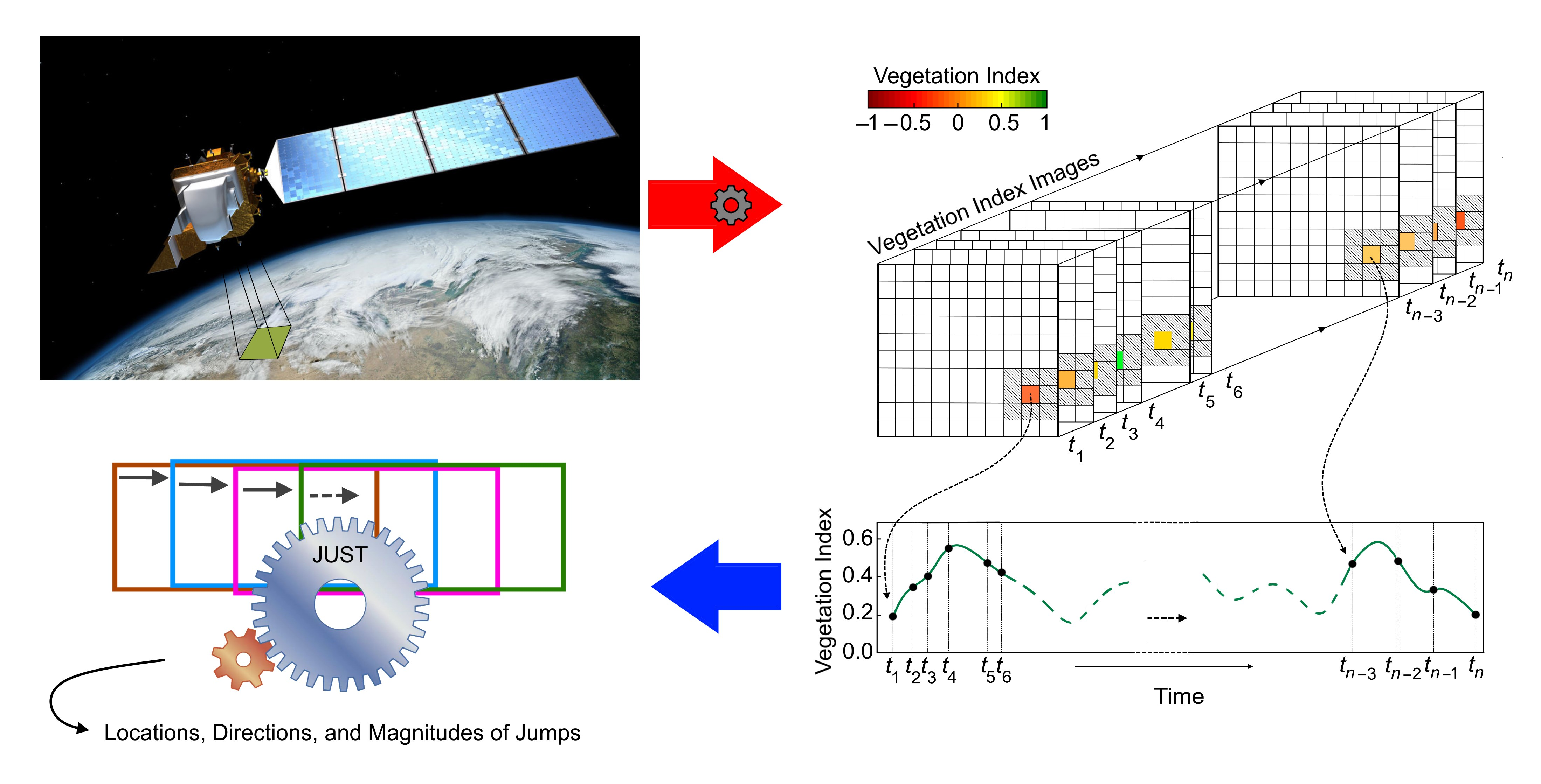
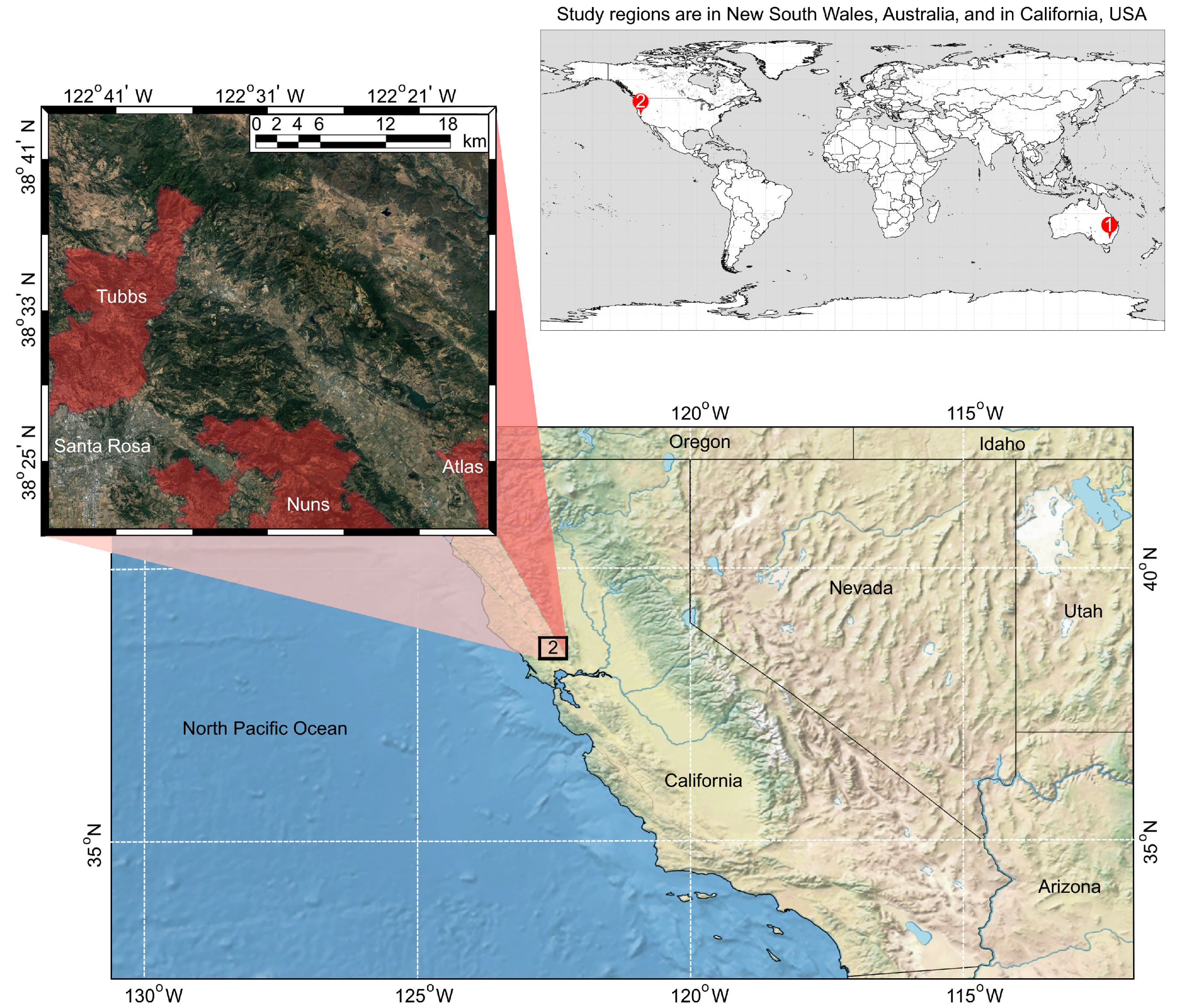
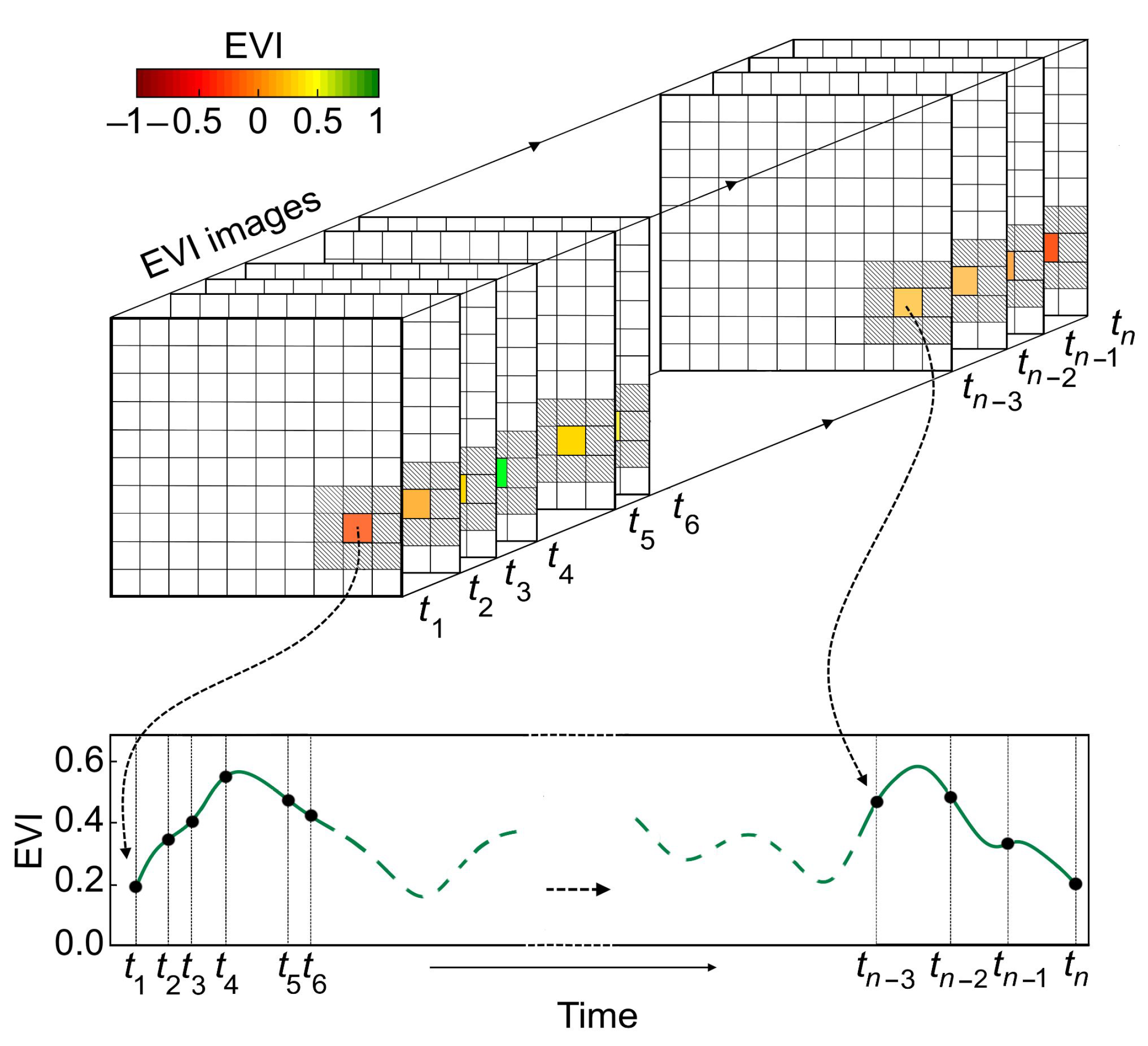
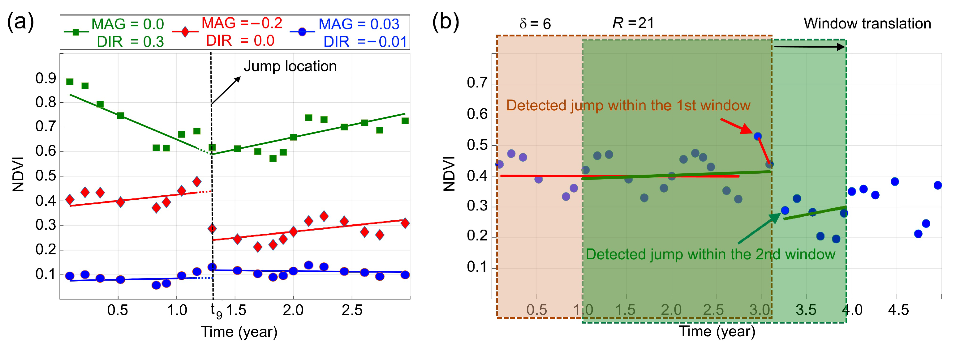
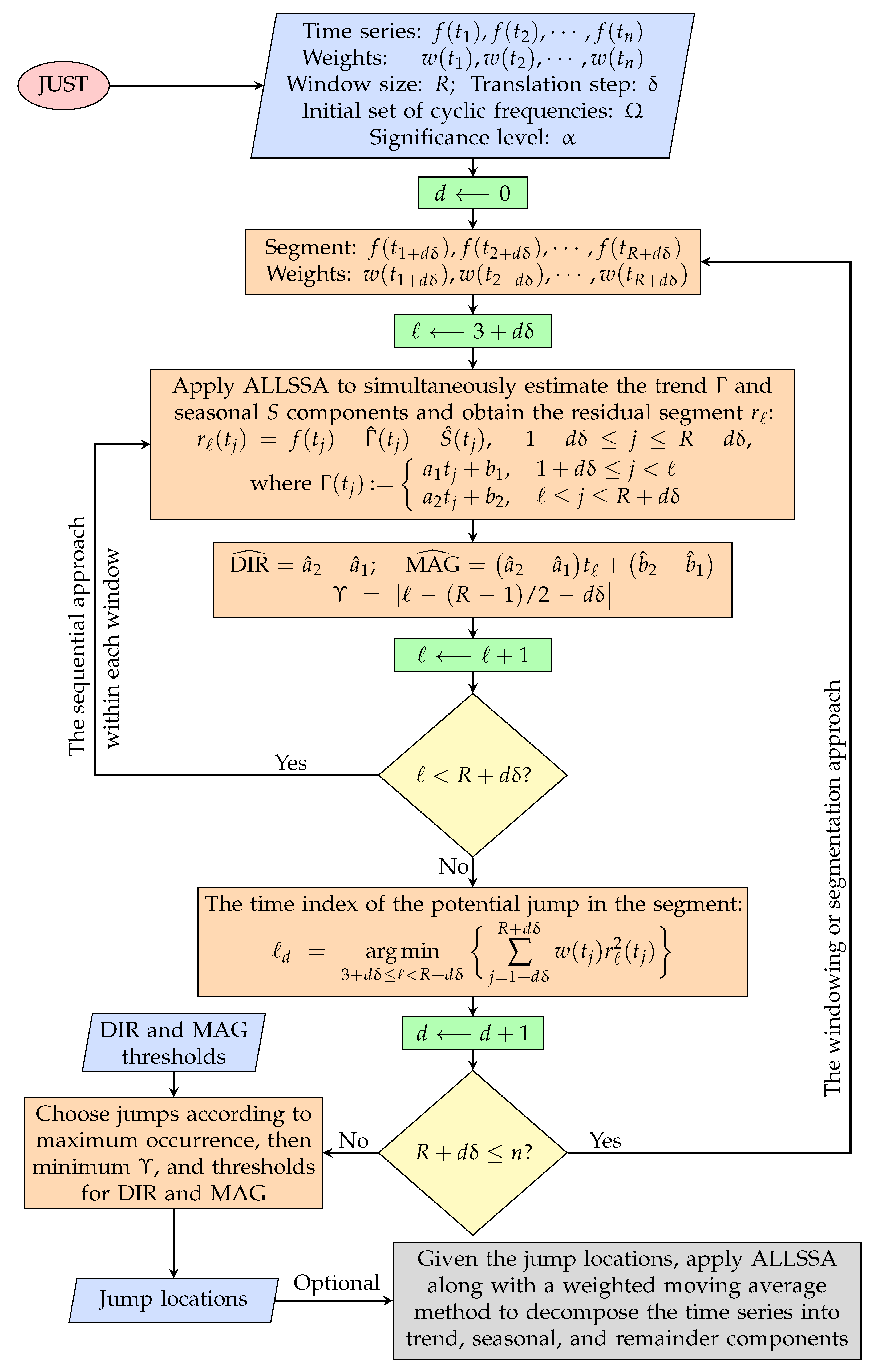
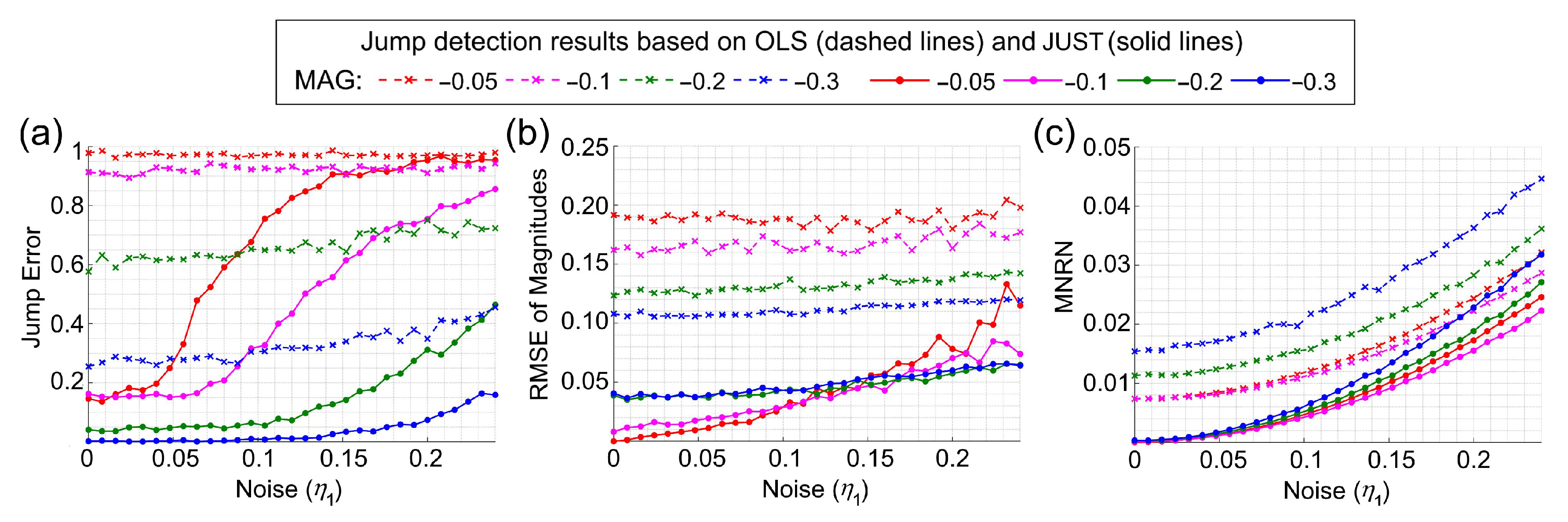
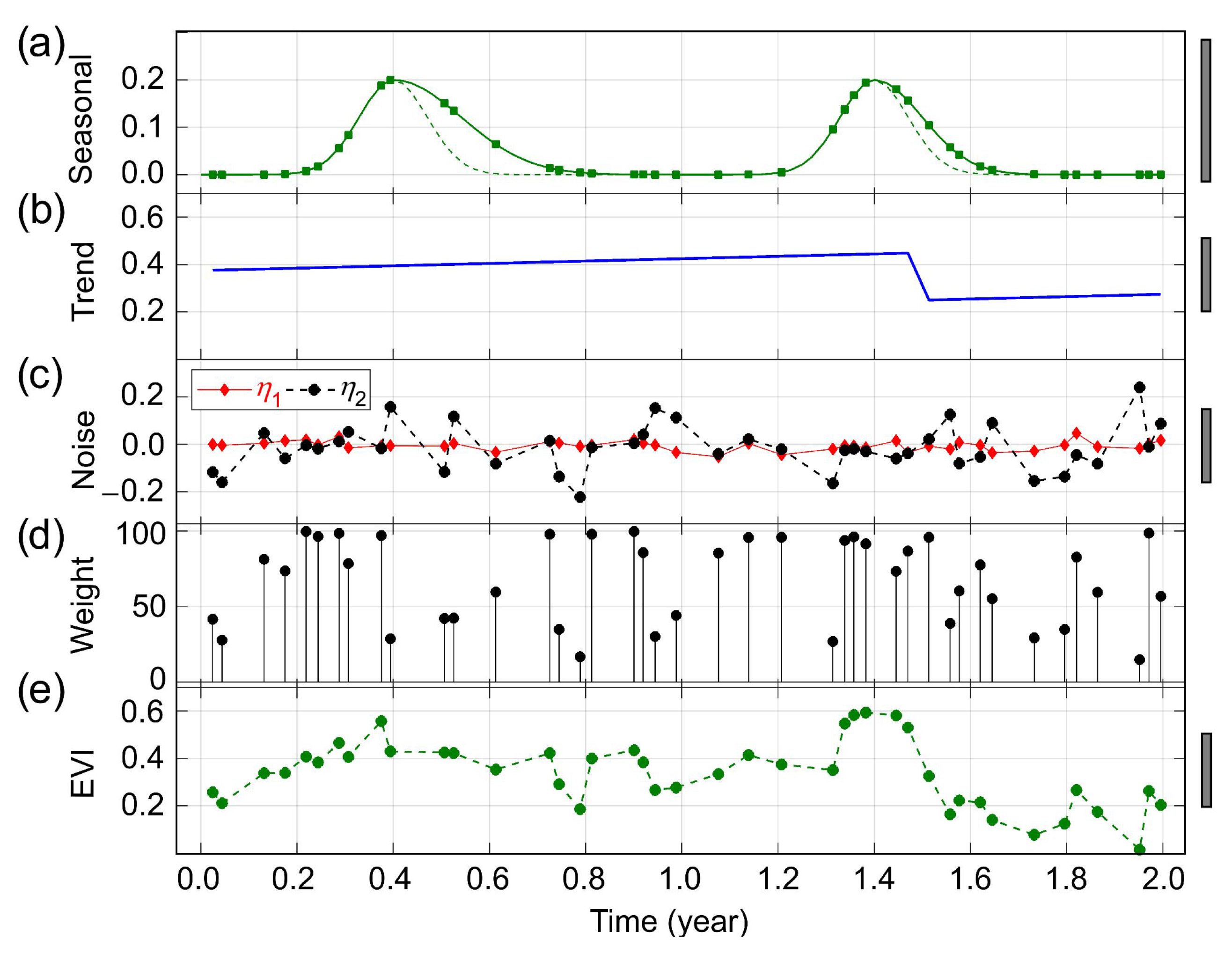
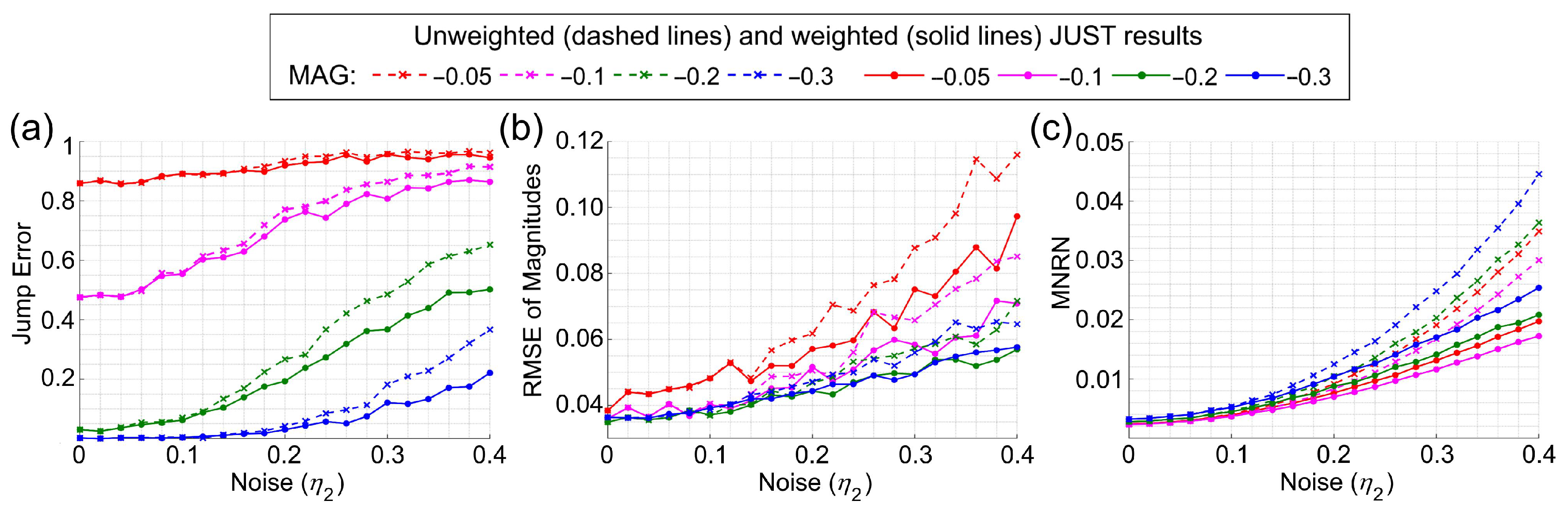
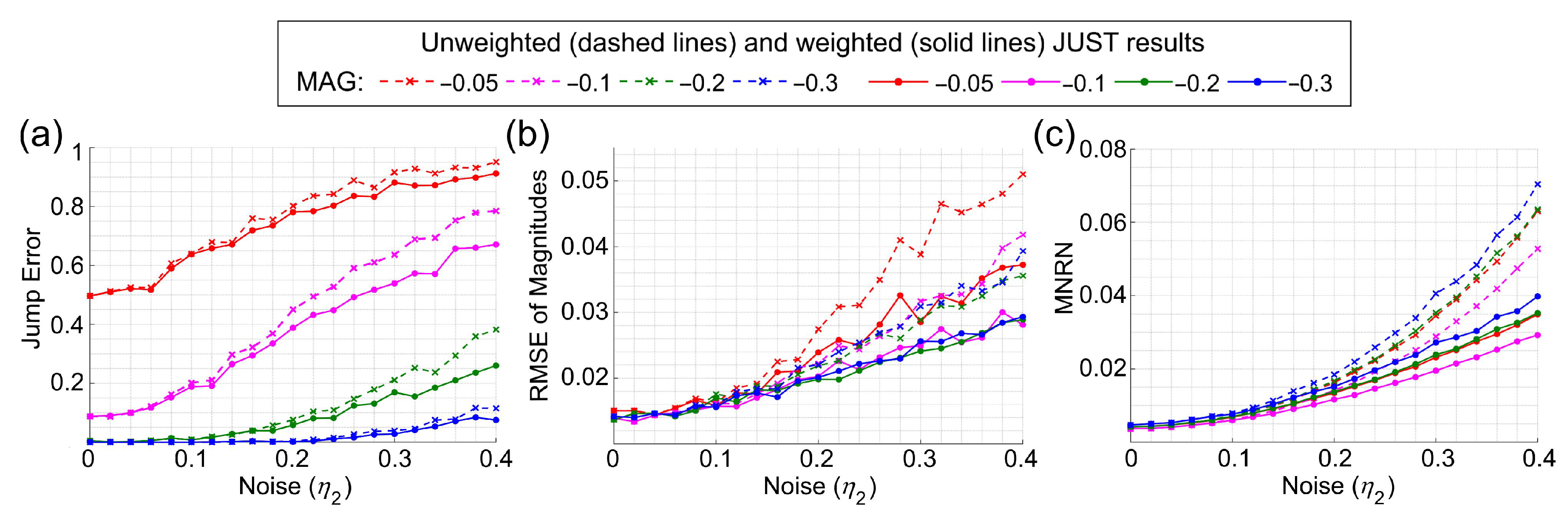
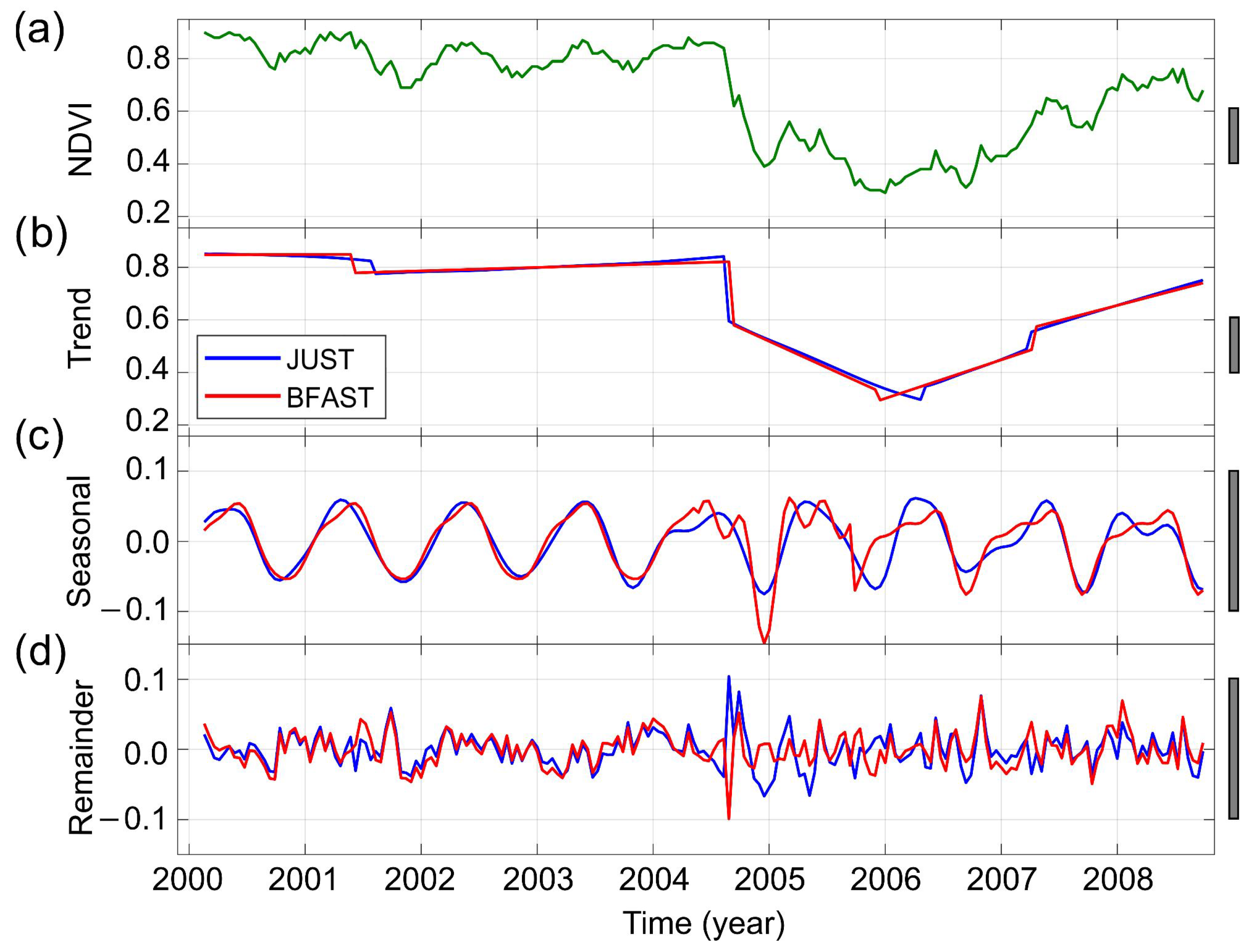
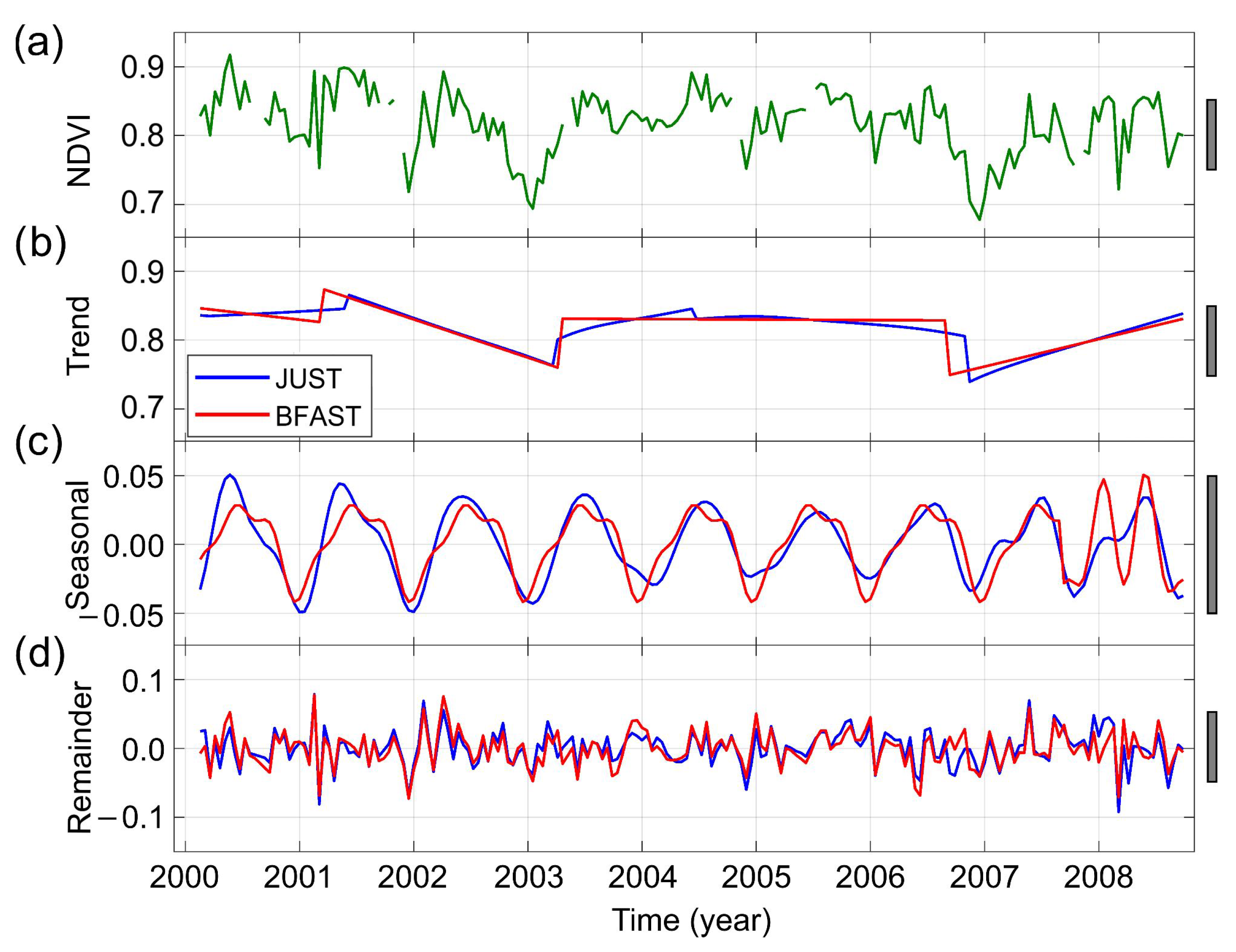
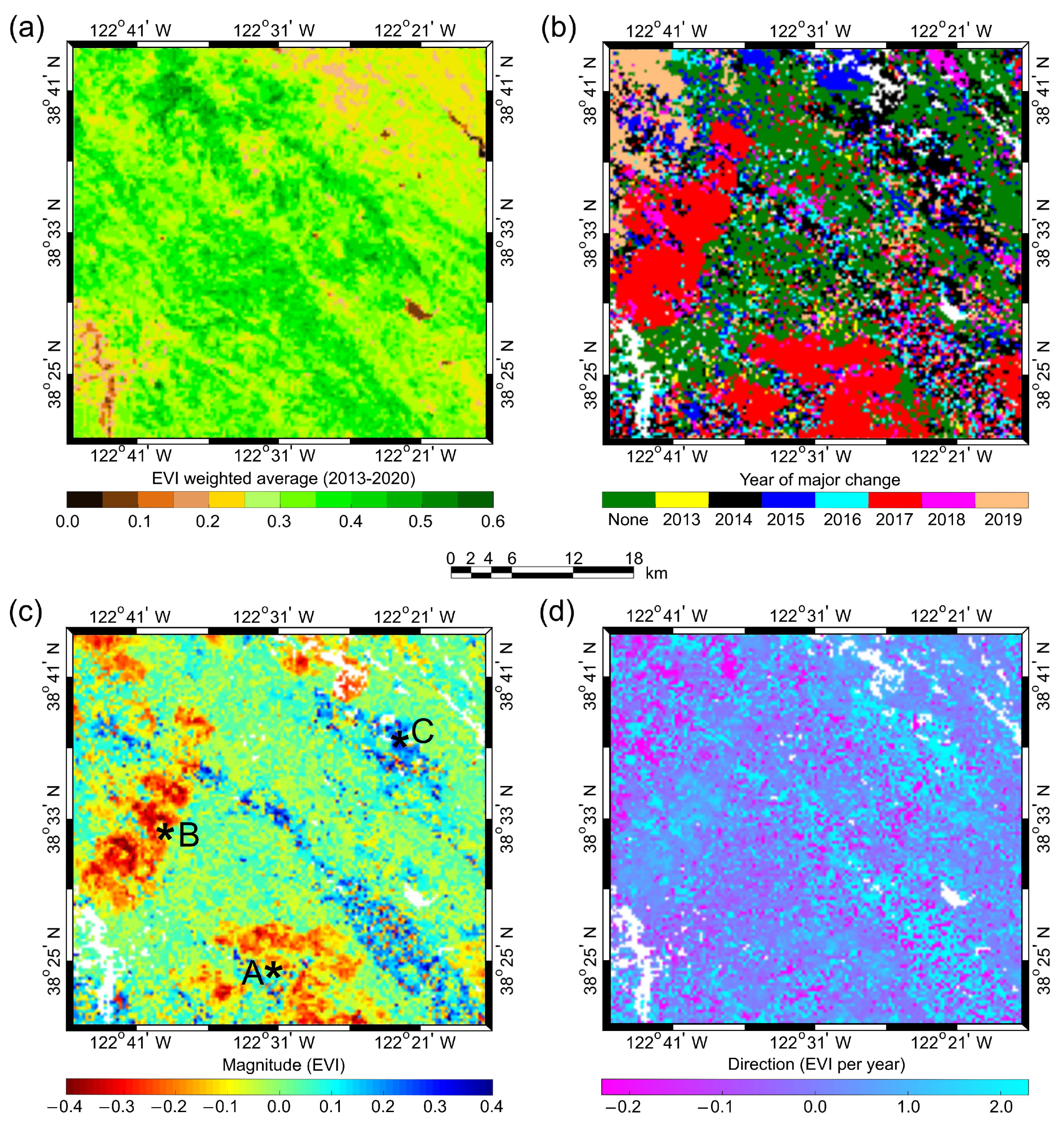
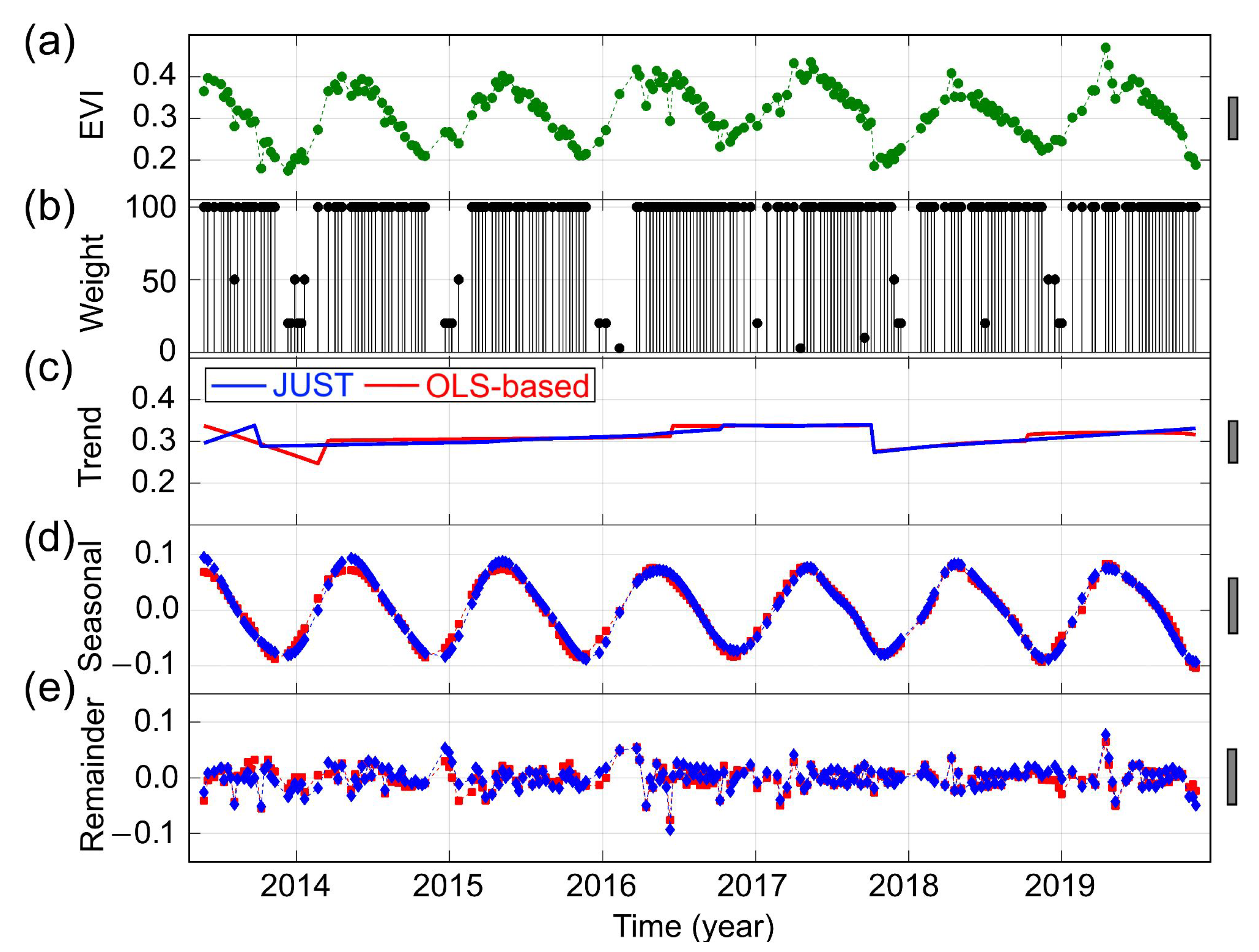
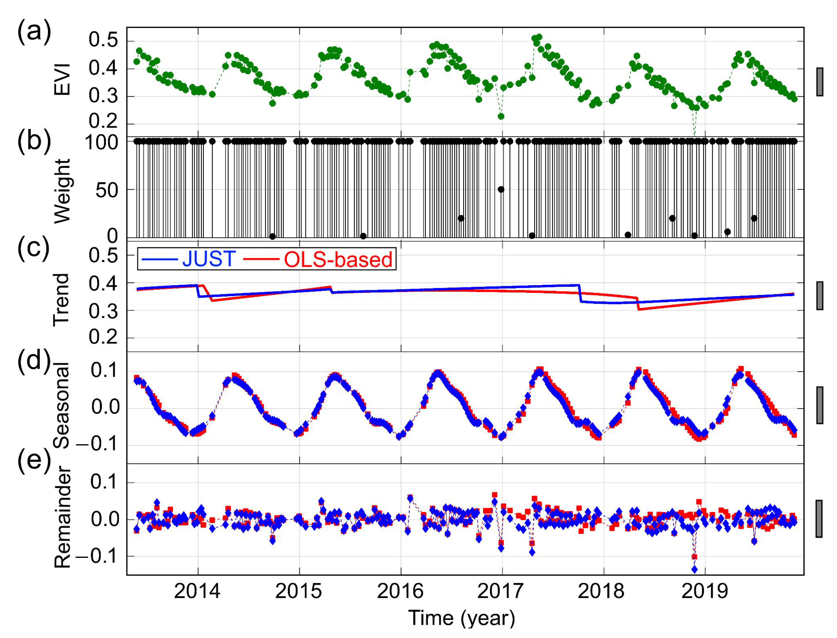
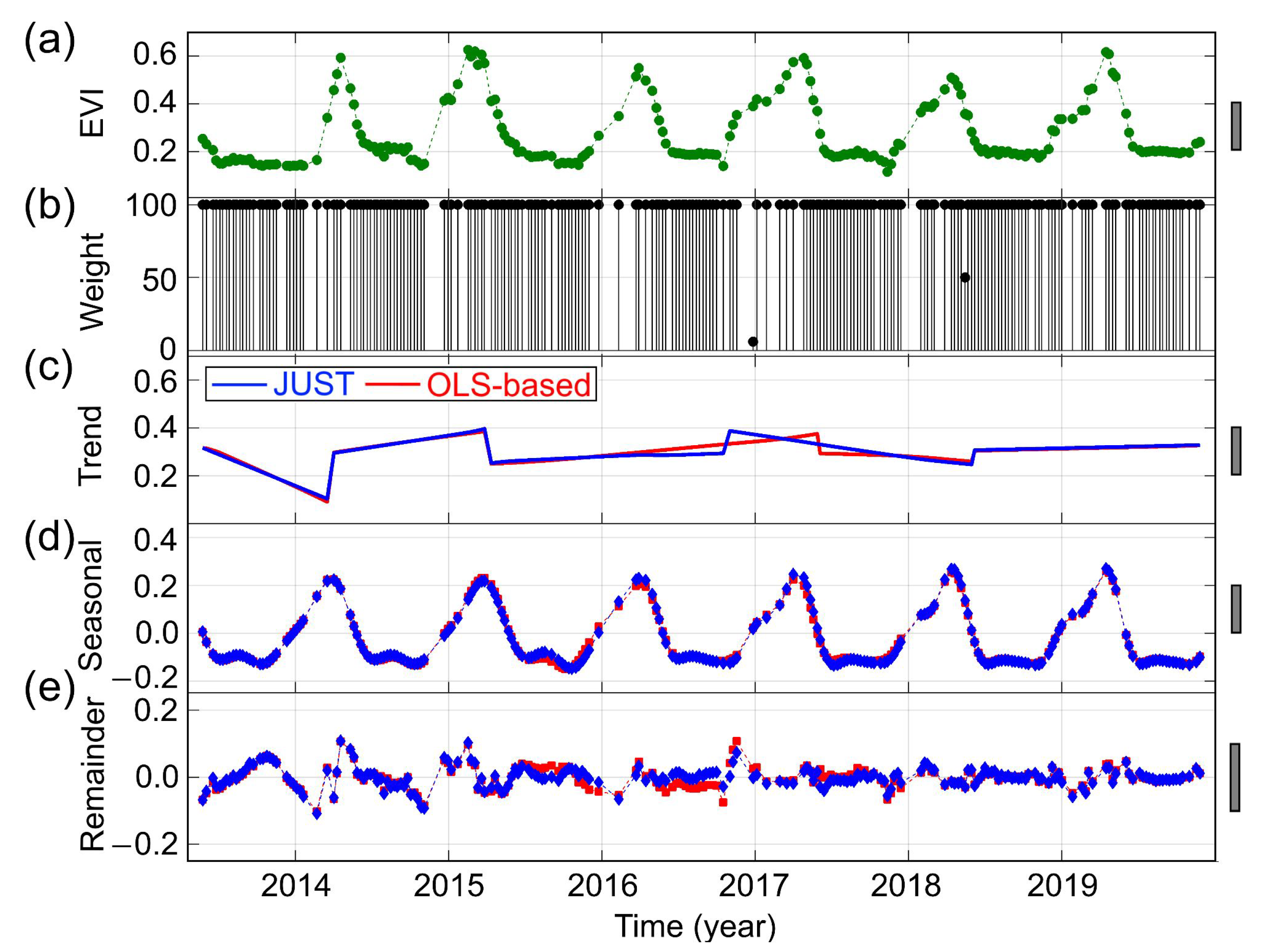
Table 1.
Main inputs and outputs of JUST.
| Inputs | Description | Default |
|---|---|---|
| t | Time values | |
| f | Time series values | |
| Weight matrix | None | |
| R | Window size | Sampling rate tripled: |
| Translation step | Sampling rate: M | |
| Cyclic frequencies | ||
| Constituents | Known forms | Linear trend |
| Significance level | ||
| Outputs: the estimated jump locations, and their directions and magnitudes; | ||
| the estimated trend, seasonal, and remainder components | ||
Table 2.
Parameter values for simulation of the linear trends in Equation (8) to compare JUST with the OLS-based method for jump detection.
Table 2.
Parameter values for simulation of the linear trends in Equation (8) to compare JUST with the OLS-based method for jump detection.
| MAG | ||||
|---|---|---|---|---|
Table 3.
Parameter values for simulation of the trend in Equation (8) to compare JUST with BFAST.
Table 3.
Parameter values for simulation of the trend in Equation (8) to compare JUST with BFAST.
| MAG | ||||
|---|---|---|---|---|
Table 4.
Comparison between JUST and BFAST for the time series simulated by the seasonal component given in Equation (7) with trend coefficients given in Table 3 and added noise. N/A means no answer. Please note that in this example the jump (break) with zero magnitude has positive direction.
| Noise Level () | ||||||
|---|---|---|---|---|---|---|
| Method | Jump Error | |||||
| JUST | ||||||
| BFAST | ||||||
| JUST | ||||||
| BFAST | ||||||
| JUST | ||||||
| BFAST | ||||||
| Method | RMSE | |||||
| JUST | ||||||
| BFAST | N/A | N/A | ||||
| JUST | ||||||
| BFAST | N/A | |||||
| JUST | ||||||
| BFAST | ||||||
Table 5.
Comparison between JUST and BFAST for the time series simulated by the asymmetric Gaussian function in Equation (11) with trend coefficients given in Table 3, and added noise. Please note that in this example the jump (break) with zero magnitude has positive direction.
| Noise Level () | ||||||
|---|---|---|---|---|---|---|
| Method | Jump Error | |||||
| JUST | ||||||
| BFAST | ||||||
| JUST | ||||||
| BFAST | ||||||
| JUST | ||||||
| BFAST | ||||||
| Method | RMSE | |||||
| JUST | ||||||
| BFAST | ||||||
| JUST | ||||||
| BFAST | ||||||
| JUST | ||||||
| BFAST | ||||||
Publisher’s Note: MDPI stays neutral with regard to jurisdictional claims in published maps and institutional affiliations. |
© 2020 by the authors. Licensee MDPI, Basel, Switzerland. This article is an open access article distributed under the terms and conditions of the Creative Commons Attribution (CC BY) license (http://creativecommons.org/licenses/by/4.0/).
Share and Cite
MDPI and ACS Style
Ghaderpour, E.; Vujadinovic, T. Change Detection within Remotely Sensed Satellite Image Time Series via Spectral Analysis. Remote Sens. 2020, 12, 4001. https://0-doi-org.brum.beds.ac.uk/10.3390/rs12234001
AMA Style
Ghaderpour E, Vujadinovic T. Change Detection within Remotely Sensed Satellite Image Time Series via Spectral Analysis. Remote Sensing. 2020; 12(23):4001. https://0-doi-org.brum.beds.ac.uk/10.3390/rs12234001
Chicago/Turabian StyleGhaderpour, Ebrahim, and Tijana Vujadinovic. 2020. "Change Detection within Remotely Sensed Satellite Image Time Series via Spectral Analysis" Remote Sensing 12, no. 23: 4001. https://0-doi-org.brum.beds.ac.uk/10.3390/rs12234001
Note that from the first issue of 2016, this journal uses article numbers instead of page numbers. See further details here.