1. Introduction
Around the world, the effects of changing plant phenology are evident in many ways: from earlier and longer growing seasons to altering the relationships between plants and their natural pollinators [
1,
2,
3]. Remote sensing techniques allow us to detect subtle changes in plant phenology, and here we present a novel approach to describe phenological cycles of mangrove ecosystems. We contribute to a better understanding of mangrove phenology by investigating physical changes of mangrove ecosystems and how the evidence of change is captured by satellite images. Accurately modelling and predicting mangrove phenology will help us understand not only the seasonal variations but also the long-term trends in the natural cycles of these forests. New models, such as the one presented here, will advance our understanding of how drought, heatwaves and other extreme weather events affect mangrove health and growth. Similar to using sea temperature to predict coral bleaching events, we could use phenology to predict mangrove dieback events akin to those of 2015 and 2016 in the Gulf of Carpentaria in northern Australia.
Phenology is related to the life cycle events of plants and animals and their relationship to climatic and other abiotic factors [
3,
4]. Plant phenology also plays an important role in the carbon cycle in the form of sequestration and storage. Phenological cycles of plants ensure that leafing, flowering and fruiting events occur during the most appropriate season to achieve maximum growth and reproductive success. Mangrove phenology is often described at the species level by relating the time of year when trees flower, fruit or defoliate with suspected drivers like temperature and rainfall [
5,
6]. For example, [
7] described the phenology and distribution of
Avicennia marina mangroves along the Australian coastline, and [
8] described the flowering and leafing phenologies of mangroves in the Darwin region. While these descriptions provide a very valuable baseline for comparison, they often lack the spatial extent and frequency needed for phenological studies [
9].
We can monitor mangrove phenology using remote sensing or we can collect in situ data. The main advantage of in situ monitoring is that it provides information at the tree and species level, where observations can be very detailed over a wide range of variables. However, in situ monitoring is challenging, time-consuming and variation in methods and survey effort can make it difficult to compare results [
10]. In contrast, the remote sensing approach provides information at the landscape and continental scales and is consistently acquired over time and space [
9]. While many studies used space-borne sensors to map mangroves at the global [
11,
12], continental [
13,
14], and local scales [
15], few have used these sensors to monitor mangrove phenology. [
16] used MODIS (Moderate Resolution Imaging Spectroradiometer) data between 2000–2014 to detect mangrove phenology using four different spectral indices in the Yucatan peninsula in Mexico. Similarly, [
17] compared the phenology of mangroves to that of the surrounding forests using MODIS imagery. While the temporal resolution of the MODIS sensors is very high (1–2 days), the spatial resolution is coarse (250–500 m). Landsat satellites offer a better spatial resolution at the cost of a lower temporal resolution. Despite this tradeoff, the Landsat archive is key to using remote sensing to monitor mangrove phenology as it provides more than 30 years of imagery at a spatial resolution of 30 m x 30 m and a temporal resolution of 8–16 days [
18].
To date, most studies on plant phenology have used fully parametric models, mainly in the form of double logistic or sinusoidal functions [
19,
20,
21]. These functions may perform well in deciduous or temperate forests, where there is a single, well defined period of leaf production, and a single, well defined period of leaf senescence [
22,
23], but these methods may not be well suited for mangroves and other evergreen forests. When detecting phenology, one of the main limitations of parametric models (e.g., logistic functions) is that they fail to detect asymmetric trends in leaf growth or senescence [
22]. Considering that the growing season of some evergreen forests consists of two periods of leaf growth and death, fully parametric (or model-driven) models have the potential to oversimplify the phenology of these ecosystems. Other, more complex models have also been used to examine plant phenology, mainly in the form of artificial neural networks, however, these methods are known to have mostly been used in croplands [
24]. Semi-parametric (or data-driven) models, on the other hand, may be better suited for this task as they do not necessarily assume that there will be a single peak or trough in leaf growth or death. Rather, semi-parametric models use the data to determine the shape of the phenology.
Studies have documented the dual phenology of mangroves [
6] and other evergreen forests [
25] in the field, but this dual phenology has not been recorded using satellite imagery. Dual phenology refers to two periods of leaf growth; unlike deciduous forests which grow their leaves during the spring, some evergreen forests have two periods of leaf growth every year. In mangrove forests these events have never been documented using satellite imagery, probably due to the use of fully parametric models to detect phenology, or because in situ data collection focuses mainly on litterfall rather than leaf production. The novelty of this study is that we use a semi-parametric method to model mangrove phenology and in doing that we present, for the first time, these two distinct periods of leaf growth described in the literature.
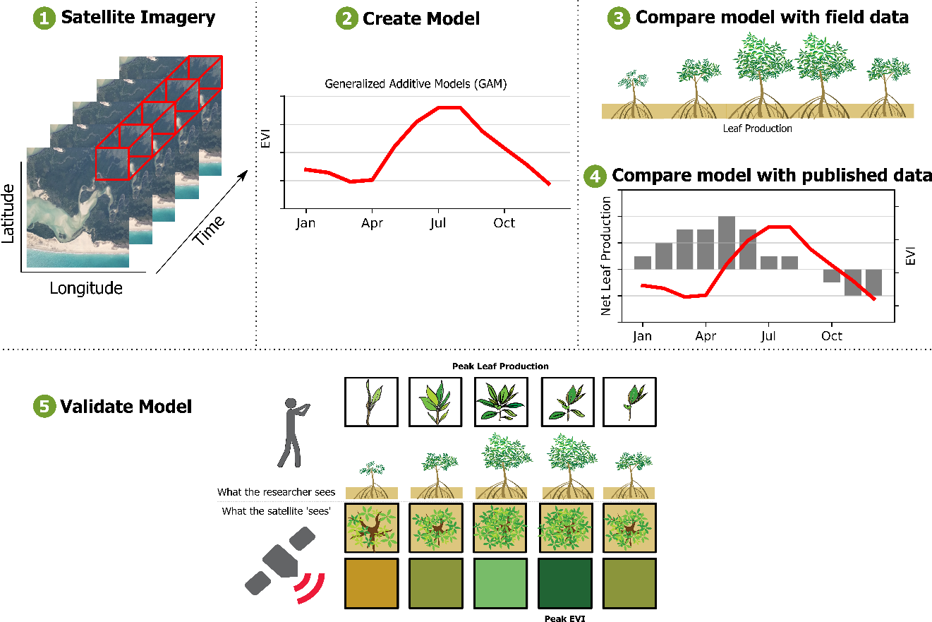
Generalized Additive Models (GAMs) are commonly used in ecology and climate sciences, to examine non-linear relationships between response and independent variables. Here we present a novel, data-driven method to extracting mangrove phenology from a series of Landsat images. We use discrete observations of mangrove forests (i.e., satellite images) and Generalized Additive Models (GAMs) to create a continuous curve of phenology over time, without assuming a certain shape, amplitude, or frequency. Our aims are to (1) use a semi-parametric approach (GAMs) to examine if seasonal changes in biophysical variables are related to seasonal changes in the spectral reflectance of mangrove forests; (2) compare the satellite-derived phenology with a set of field observations and measurements; (3) compare the satellite-derived phenology to peer-reviewed literature describing the phenology of mangrove forests, and (4) determine how the Enhanced Vegetation Index (EVI) responds to leaf gain, leaf fall or net leaf production in mangrove ecosystems across Australia.
This manuscript is organized in the following way: firstly, we describe the site and methods used to collect the field data. Then we describe how we use the literature to create a proxy for mangrove phenology. Afterwards, we describe the use of GAMs and satellite images to detect the apparent phenology of mangroves across northern Australia. Having done this, we present the models of apparent phenology and compare them with the data collected in the field, and the proxies from the literature. Finally, we discuss the results, limitations, and future work.
2. Materials and Methods
We selected six study sites across Australia to evaluate mangrove phenology from satellite imagery using GAMs. One site corresponds to field observations collected in the Gladstone region (Queensland) in the late 1990s, and the remaining sites (
n = 5) correspond to qualitative data extracted from peer-reviewed publications (
Figure 1). In this section, we first describe the field site followed by the peer-reviewed studies, the image acquisition process, and the time series analysis using GAMs. Finally, we describe the phenology model validation.
2.1. Field Site Description
The Gladstone region in central Queensland is home to over 100,000 ha of intertidal wetlands, out of which 30% are mangrove forests [
26]. The annual mean temperature ranges between 18.4 °C and 27.5 °C, the mean annual rainfall is 874 mm, and the semi-diurnal tides often range from 1.5–3.5 m but reach up to 6 m. In this region, mangroves of the
Rhizophora, Avicenna, and
Ceriops genera are among the most common [
5,
27]. The field data were collected between July 1996 and August 1998 in two plots located in Fisherman’s Landing and one plot on Curtis Island (
Figure 2). The sites were dominated by
Rhizophora stylosa trees and located within the Landsat World Reference System 2 (WRS-2) path 91 and rows 76 and 77.
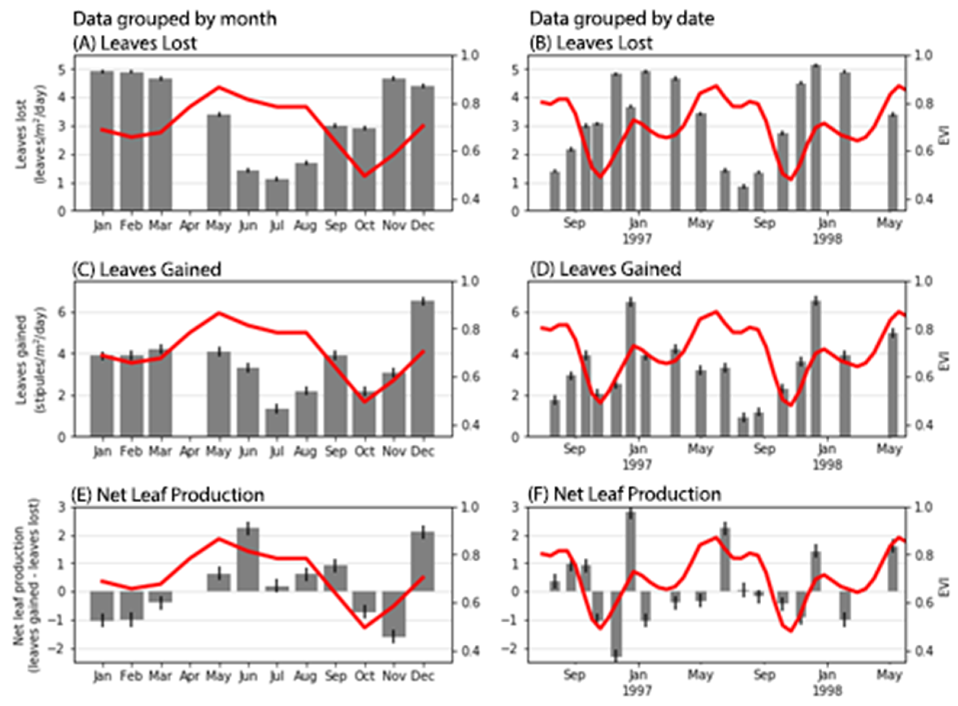
2.2. Field Observations and Measurements
The data were collected by [
26] in the following way: in each plot, the authors selected mature
R. stylosa trees between 4–9 m tall and tagged 21 leafy shoots in the upper two meters of the canopy totaling around 378 shoots. The authors conducted monthly inspections and recorded the shoot growth, number of leaves, reproductive parts and number of branch shoots. To measure the amount of litterfall, the authors suspended litter traps (1 m
2 in area) under the selected trees. The traps were suspended above the high tide mark and litter was collected, sorted and weighed on a monthly basis. During the data collection period, the average tide height was 2.49 m according to the historical record for the site [
28]. Importantly, [
26] never intended to validate satellite imagery with their data, therefore (1) no spectral data were collected, making these data completely independent from the satellite-derived phenology, and (2) we do not anticipate a high correlation between satellite-derived phenology and the field data. The data consist of the mean monthly values of six phenological variables, however, we selected the three that were more relevant for our study (see ([
26], pp 105–108) for details). The selected biophysical variables are detailed below:
Leaves lost [leaves × m−2 × day−1]: The number of leaves that fell into the litter traps.
Leaves gained [stipules × m−2 × day−1]: The number of stipules that fell into the litter traps. This variable serves as a proxy for the number of leaves produced in a tree.
Net leaf production [leaves gained-leaves lost]: The difference between leaves gained and fallen leaves. This measure is an indication the net balance of leaves in the canopy with more or less leaves as leaves appear or fall, leaving the canopy in either debit (=stressed), credit (=growth) or neutral condition.
2.3. Published Literature on the Phenology of R. stylosa
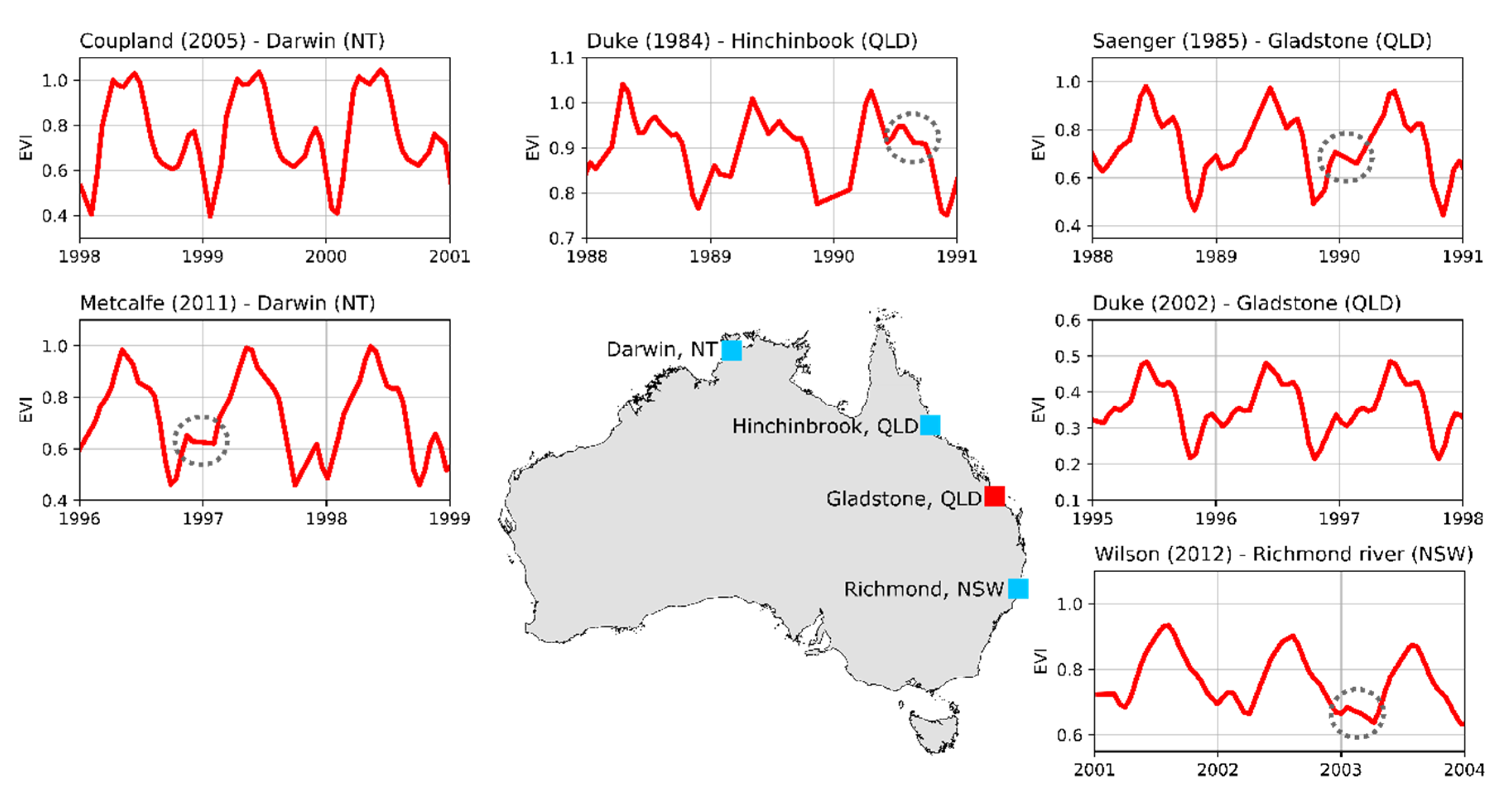
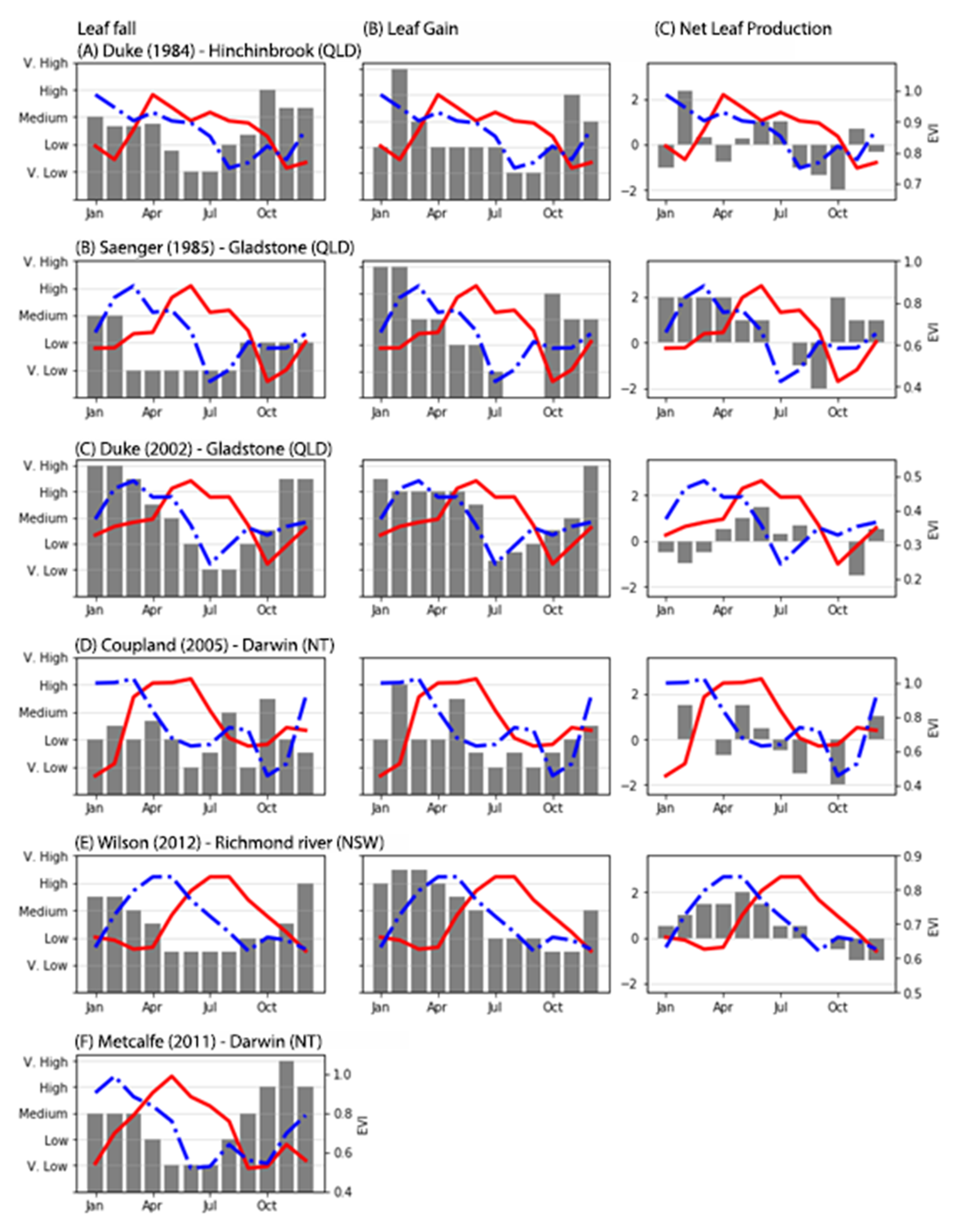
To compare the apparent phenology (i.e., from the GAMs) to other sources of information, we gathered a set of peer-reviewed papers that included
R. stylosa as target species. The reasons for selecting this species were twofold: (1) it is common throughout northern Australia; (2) a number of studies have described its phenology over a wide geographic area across the Indo West Pacific region. We looked for papers that had a graphical interpretation of leaf fall and/or leaf gain over time and we found six examples (
Table 1). We used the published graphical interpretations of leaf fall and leaf gain to determine, in a qualitative way, the times of the year where most leaves grew or fell. All published graphs show “Time” on the horizontal axis and a measure of leaf fall or gain on the vertical axis. In each study, we divided the vertical axis into five equidistant categories (i.e., very low, low, medium, high, very high) and recoded the category for each month (not shown). Finally, we calculated the net leaf production from each study by subtracting the leaf fall from leaf gain values and then compared the three variables with the apparent phenology of each site (
Table 1).
From
Table 1 one can see that the studies by [
29,
30] predate the time where Landsat imagery was collected. Between 1974 and 1989, cyclones Dawn (March 1976), Keith (January 1977), Gordon (January 1979), and Kerry (March 1979) affected Hinchinbrook Island, Gladstone, or Proserpine in Queensland. Neither [
29] nor [
30] mention the effects of cyclones, drought on their respective study sites, either because the field campaigns happened before the cyclones, or there was no significant damage to the trees. While there is no certainty about the effects of extreme weather events for those studies, here we assume that the phenology observed by the authors did not change until satellite imagery was acquired.
2.4. Landsat Image Acquisition and Processing
Digital Earth Australia holds a copy of the Landsat archive (1987–present) for the whole of Australia [
18,
34]. Digital Earth Australia provided all L1T images (
n = 668) of our sites between 1987 and 2006 for the Landsat 5 (TM) and Landsat 7 (ETM+) sensors, and performed (1) geometric, (2) atmospheric and (3) Nadir-adjusted Bidirectional reflectance distribution function Reflectance (NBAR) corrections following [
35]. All corrections were performed within Digital Earth Australia, using the python programming language. Digital Earth Australia uses the ‘Pixel Quality Assessment’ algorithm [
18] to remove pixels with clouds and cloud shadows, as well as all missing pixels resulting from the Landsat 7 Scan Line Corrector failure; these pixels were removed from the datasets and not used (i.e., there was no gap-filling for ETM+ data). The main reason for not filling the missing pixels is that we wanted to use the GAM with only true values, rather than including additional uncertainty to the GAMs. Having done this, we calculated the Enhanced Vegetation Index (EVI) [
36] for each pixel in each image. We chose EVI because studies show that this spectral index does not saturate with high vegetation densities [
36], it is better suited than other indices for discriminating vegetation fraction in mangrove ecosystems [
37], and it is commonly used for phenology investigations [
16,
17].
Our study leverages the high temporal density of the Landsat archive, and the overlapping footprints of two or more Landsat scenes, hence increasing the number of usable pixels in a given area. On average, the difference between the dates when field data was collected and the closest satellite image acquired is 5 days, as shown in
Table 2. To compare the GAMs with peer-reviewed literature, we selected a period equal to the time of the data collection plus and minus one year, thereby ensuring that the models had enough input data. In the cases where studies were dated before 1987, we used the first three years of available imagery of the area to create the GAM (
Table 1). We estimated the location of the studies from the site descriptions in each publication and created a region of interest of approximately 17 ha of mangrove forests surrounding the study area. Afterwards, we selected only the pixels that corresponded to mangrove forests using the “Mangrove Canopy Cover” product developed by Geoscience Australia ([
13]) and applied the GAM to every pixel within our region of interest. This approach ensured that we captured the phenology of the mangrove community instead of a small plot.
2.5. Time Series Analysis Using Generalized Additive Models
With all images pre-processed, georeferenced and sorted by time of acquisition, we proceeded to create a model of phenology for every available pixel in our study sites using GAMs. Contrary to linear additive models, GAMs are statistical models in which the relationship of predictor and response variables is captured by smooth functions instead of coefficients [
38]. Equations (1) and (2) show the respective linear and generalized additive relationships between one response variable
and two predictor variables
for
i observations [
39]:
Noticeably, there is no change in the form of the model, however, there is no assumption that the relationship between predictor and response variables is linear. In Equation (1) an additive linear relationship between
and
is captured by the slope terms
and
, while in Equation (2) the additive relationship is captured by the “smooth” functions
and
. The shape of the “smooth” functions (
, also known as “splines” or “smooth splines”, is determined during the computation in an iterative way and can take many forms (e.g., polynomial, linear, quadratic) [
39,
40]. Each ‘smooth’ function (
), or spline, is comprised of several basis functions (
bn), their coefficients (
), and where
K determines the maximum complexity of each smooth function:
As explained by [
41], GAMs use several types of splines to determine the relationship between each predictor variable (
) and the response (
) is evaluated at every data point in an iterative way, for every predictor variable (see [
42] a detailed description). In this case, and following [
43], the base function is a Fourier basis with 2N parameters
, that allow the construction of a matrix of seasonality vectors for each past and future value of
t. Importantly, we are neither fitting a Fourier series to the data, nor assuming that the relationship of EVI and time is symmetric. Here, the apparent phenology of each pixel results from the Fourier basis expansion evaluated at each data point, and adding the weighted basis functions. In summary, the detecting apparent phenology is a curve-fitting exercise rather than a time series decomposition one.
Another characteristic of GAMs is that measurements do not need to be evenly spaced in time [
43]. This works well in our case for two reasons: (1) pixels with clouds, shadows and other errors are flagged as invalid observations leading to time series with random gaps in both length and timing; and (2) areas where the footprints of two or more scenes overlap will have more observations than areas with no overlap.
To detect mangrove phenology from a satellite-derived data series, we used the Python programming language and the “Prophet” package (version 0.3.post2) developed by Facebook [
43]. Facebook designed this package to analyze user engagement with the social network at different time scales, and to investigate how periodic events such as holidays affect that engagement. Similar to mangrove phenology, user engagement on the social media platform is affected by regular and irregular events such as weekends (i.e., regular events) and public holidays, which change every year [
43]. In a similar fashion, mangroves are affected by regular changes in temperature and rainfall (i.e., seasons) and irregular events such as cyclones or drought. While the time scales may differ, the concept of tracing an event (e.g., phenology or user engagement) over time remains the same. We selected this package due to its ease of use and re-purposed it to extract seasonal variations in greenness and phenological metrics from satellite images of mangrove forests.
2.6. Phenological Metrics
With the data ingested, Prophet separates the seasonal components of the time series from the trend and the residual components. The seasonal component of the GAMs is used as an approximation of phenological cycles and several techniques can be adapted to extract the start, end, and duration of the mangrove “green-up” season. In this study, we adopted similar definitions to those by [
44] to identify the Start of Season, End of Season and Peak Growing Season, however, as our study does not involve a sinusoidal curve the definitions vary slightly. For simplicity, we define the start of season and end of season as the lowest points, and peak growing season as the highest points of the de-trended time series (
Figure 3). We also define the length of the growing season as the time between the start of season and end of season. Because we use start of season, end of season and peak growing season as phenological metrics of the landscape, they do not represent individual species.
We extracted the start of season and peak growing season for each pixel in our field study site in the following way: from the seasonal component, we selected the predicted index values from the GAMs that were lower or higher than the 5 or 95 percentile as the potential start of season or peak growing season dates, respectively (
Figure 3C). Then we selected the median of the image acquisition dates as the start of season, peak growing season and end of season dates. In case the selected date was not a date in which an image was acquired, we searched for the image with the closest date and used that date instead.
Because we wanted to determine if the GAMs were correlated with biophysical processes described in the literature (i.e., leaf gain, leaf loss, net leaf production), we decided to shift the models (i.e., displace the models along the time axis) by one, two and three months. We then examined if the EVI response was immediate or delayed. An immediate response of EVI to a biophysical process would imply that remote sensing techniques could be used for real-time monitoring. In contrast, a delayed response would help us understand which processes drive the changes in EVI. After comparing the biophysical processes to the EVI, we examined their relationship using linear regressions.
2.7. Validation of the GAMs
We assessed the precision of our model by running linear and non-linear regressions between the apparent phenology and (1) observed EVI values from satellite imagery; (2) in situ data from [
26]; and (3) leaf fall, leaf gain and net leaf production values from published literature. We did this using the Scikit-Learn package for python [
45], specifically, we used simple linear regressions and support vector regression with linear, polynomial and radial basis function kernels. We chose support vector regression because it is robust against outliers, it is easily implemented, and it allowed us to compare linear and nonlinear relationships between apparent phenology and the data measured in the field. In addition, we performed 5-fold cross-validation using the performance metrics functionality provided by “Prophet” (see the
Supplementary Information section, Figure S2.
4. Discussion
Extracting phenological metrics of mangrove forests from satellite images is an ongoing field of research. We contribute to this field by (1) presenting a novel, data-driven method to extracting phenology from satellite imagery; and (2) applying the method in evergreen forests across Australia. We also expand this field of research by presenting the dual phenology of mangrove forests, as described in the literature. By demonstrating that there is more than one period of leaf growth in these ecosystems, we also highlight the need for deeper investigation into the detection and causes of dual phenology in evergreen forests and the need for long term field studies that validate satellite observations. Importantly, with the use of satellite images, we have demonstrated that plots with similar species can have different phenologies. Phenology is, in turn, site-dependent and hence should not be described using a single logistic or sinusoidal curve.
Because phenology is site-dependent, methods like the one presented here can be used with long term imagery archives to determine the baseline of mangrove phenology in stable ecosystems, and compare it to stressed ecosystems. Early detection of ecosystem stress, indicated by changes in phenology, could lead us to detect, predict, and hopefully prevent, mangrove dieback events.
4.1. The Phenology of Rhizophora Stylosa
Authors have described, in situ, the phenological traits of
R. stylosa around the world, however, few have attempted to compare mangrove phenology across regions. [
16], for example, used satellite imagery and a sinusoidal model to describe seasonal variations of mangrove forests in the Yucatan peninsula in Mexico. They found that the spectral index values are lower during the dry season and higher during the wet season, an outcome that differs from our findings. Across all our study sites, we found lower EVI values during the wet season and higher EVI values during the dry season. These differences may be due to the geographical location and the species composition of both studies.
R. mangle,
Laguncularia racemosa,
Avicennia germinans and
Conocarpus erectus dominated their study site, while
R. stylosa, A. marina and C. tagal dominated ours. Despite
R. stylosa being the dominant species in our site, several species of mangroves may contribute to the apparent phenology of each pixel given the resolution of the Landsat images (i.e., 30 m). Determining the contribution of each species to the apparent phenology is an ongoing field of research.
Another big difference between our study and that of [
16] is that the species that dominate mangrove forests in their study sites show a unimodal phenology response across the Yucatan peninsula. In contrast, we found bimodal phenology signals in our field study site, as well as in the sites described in the peer-reviewed literature (
Figure 4). This bimodal phenology is not new. [
29], and later [
6] described
R. stylosa and other mangrove species as having two distinct periods of leaf growth each year. The novelty of our analysis has allowed us to demonstrate that these two periods of leaf growth can be detected from satellite imagery using semi-parametric methods. While not all mangrove ecosystems display dual phenology, GAMs create the capability to detect it, giving researchers a tool for inductive reasoning and opening the doors for further mangrove research to validate satellite observations.
Moreover, the method presented here accounts for differences in leaf growth intensity between the sites (e.g.,
Figure 6C,E). Resolving these two periods of leaf growth is important to improve current models of carbon and water fluxes and their relationship to climate forcing. Descriptions at the plot level certainly help us understand the bimodal response of EVI over time, however, the number of leaves that a tree produces might not be the only explanation for a bimodal response in EVI.
Recently, [
46] suggested that the seasonal response of EVI in an evergreen forest was bimodal due to layers of the canopy responding in opposing seasonal patterns. When there is a decrease in leaf area index of the upper canopy, the lower canopy takes advantage of the extra light to increase its leaf area. Following the findings by [
46,
47], propose that the seasonal response of EVI comes from variations in leaf area index and photosynthetic capacity (i.e., younger, more efficient leaves), rather than from climate and weather patterns alone. Indeed, leaf ontogeny, demography and longevity could influence satellite observations, with leaves of different ages having varying amounts of chlorophyll, carotenoids, and water, resulting in slightly different spectral signatures. These assertions need to be tested in mangrove ecosystems, to determine if the bimodal response of EVI is related to the canopy structure or net leaf production.
In this study, we have demonstrated that seasonal and inter-annual changes in leaf gain and net leaf production are related to changes in EVI. [
32] suggested that leaf production of
R. stylosa in Northern Australia is most evident during the wet season (December through May), however, this species produces new leaves throughout the year. Similarly, [
33] found that
R. stylosa has the highest values of leaf production and leaf fall between December and April. The authors also indicated that this species has a net leaf gain between January and August, and a net leaf loss between September and December, which coincides with upward and downward trends in the apparent phenology for that site (
Figure 6E). Despite the strength of the apparent phenology-net leaf production relationship, when using satellite imagery, other factors affect the phenology response of mangrove forests.
Environmental and biological factors such as cyclones, rainfall and tree age are known to alter the phenology and spectral response of mangrove ecosystems [
16,
48,
49]. With the help of satellite imagery and GAMs, we can now look at inter-annual changes in mangrove phenology (e.g.,
Figure 4) and relate them to environmental or biological factors. Because these factors may change one by one, or several at a time, inter-annual predictions of mangrove phenology are difficult. A way to improve the prediction of seasonal and inter-annual phenology is to include past and present observations of these factors during the creation of the GAMs. GAMs create a numerical relationship between each factor and the phenology model to determine how influential is the former over the latter. This is an ongoing avenue of research.
Similarly, biological variables such as species composition, growth rate and forest maturity may also affect the spectral response of mangroves, and thus, any model derived from satellite sensors. A mature, dense forest will have a different response to a newly-planted mangrove patch or one that is recovering from a natural or manmade disaster [
50]. Because relating 30 years of satellite observations to biological processes requires that in situ data is collected frequently and over long periods, the need for long-term (five or more years) monitoring sites in mangrove forests is evident. Long-term monitoring of mangrove ecosystems is important, especially when relating variations in spectral indices, to changes in tree growth and temperature such as those presented by [
51,
52].
4.2. GAMs vs. Parametric Methods
Our ability to detect and forecast mangrove phenology improves our understanding of the ecosystem [
1], and our approach greatly differs from others, more commonly used [
53]. For example, [
54] derived a mathematical function that resembles the phenological phases of forests in the northeastern United States. They aimed to use satellite images to monitor vegetation dynamics at the landscape level, and one of their biggest achievements was that the method did not require any fixed constants or thresholds to be applicable. This method has been used at the local [
55] and global scales [
23], however the premise that a parametrized mathematical curve fits every plot of land has remained unchanged. The method derived by [
54] assumes that the selected model of phenology is: (1) correct, (2) already known and (3) is invariant through space and time [
39,
56]. Even recent studies [
17] insist on these assumptions when applying smoothers and filter to the data prior to detecting the phenology without considering that the data they discard may provide insights into the phenomenon they are trying to model (i.e., phenology). This in itself is not a limitation of the parametric models, but of the analysis workflow selected by the authors. We, on the other hand, used semiparametric GAMs as an estimation method to describe the changing relationship between mangrove phenology and EVI. GAMs let the data define the shape of the phenology curve, allowing for bimodality and skewness to be detected and modelled [
56].
As shown above, the relationship between EVI and mangrove phenology changes with space and time. The main limitation of parametric approaches is that those methods are constrained to the particular models evaluated (e.g., [
54,
57,
58]). That is to say, parametric methods assume that the shape of the phenological curve remains invariant and only variations in the frequency and amplitude of the signals are allowed. As demonstrated by [
46,
47] leaf demography and ontogeny can change the way we detect phenology from remotely sensed data, and as such, we need models that can tell us more than just seasonal variations in greenness. GAMs can fill this gap.
In contrast to parametric methods, GAMs use the data itself (in this case EVI values from satellite imagery) to determine the shape of the relationship. Because the relationship between the predictor and response variable is unknown beforehand, GAMs apply a series of smooth functions and use the data to determine which function is the best fit for a given dataset. This data-driven approach enabled us to demonstrate three key things: (1) the phenology response of mangroves forests dominated by
R. stylosa is not unimodal, but often bimodal across our study sites; (2) the second leaf growth phase varies in intensity depending on the site. For example, the second leaf flush is much lower in New South Wales (
Figure 6E) than in Queensland and the Northern Territory (
Figure 6B,D). The reasons behind these differences are not fully understood but may be due, in part, to differences in air temperature, rainfall and water temperature; (3) the phenology response of mangrove ecosystems is site-dependent and GAMs allow us to see small seasonal and inter-annual variations that are otherwise impossible to detect using fully parametric methods. However, to provide a better, more accurate, description of mangrove phenology we need ecophysiological descriptions that span more than 18–24 months to compare to satellite-derived phenology.
4.3. Validation of the GAMs
Peer-reviewed literature of phenological models often lacks a description of the methods used to validate the models, making it difficult to compare the performance of the GAMs versus other approaches. Despite this limitation, we validated our apparent phenology using three different, independent sources of information and found that GAMs are good tools to extract the phenology response of mangrove forests from satellite images.
Linear regressions between Observed and apparent phenology values showed a good model fit, with R
2 > 0.40 in half of our study sites despite variations in the raw EVI values (
Figure S1, see
supplementary materials). Correlation values between the GAM and in situ (
Table 3, and
Figure S1) data were low (as expected), but there are valid reasons for this. The study by [
26] focused on three sites in the Gladstone region in Queensland and aimed at examining potential bioremediation strategies in case an oil spill hit the Queensland coast. The authors never intended to use the field data to validate satellite imagery, hence the difficulties in correlating one with the other. Furthermore, the dataset consisted of one value per date per site i.e., only three data points per date, and some dates had no values (e.g., April 1997), which reduced the potential for correlation even more. Lastly, the study only gathered data over an 18-month period, limiting our information to one and a half growing seasons. Having only one full season of information limits the number of links we could create between the apparent phenology and the field data. We need longer field studies to understand fully the phenology curves extracted from satellite imagery and to examine the response of mangrove forests to changes in weather and climate patterns.
The validation of the apparent phenology with peer-reviewed literature provided us with two important pieces of information: (1) our models correlate well with the leaf gain intensity and net leaf production reported in the literature, regardless of the year in which those data were acquired; (2) apparent phenology has a two- to three-month lag with leaf gain intensity in most of our study sites. The former is important because it highlights the usefulness of GAMs. The latter tells us that, from a biophysical perspective, EVI responds to the canopy elements that absorb red light for photosynthesis and scatter near infra-red light, while field phenology traces leaf formation and drop. The delayed response of EVI is expected for two reasons: (1) the time it takes newly formed leaves to reach their maximum size, and (2) the net leaf production varies throughout the year. In
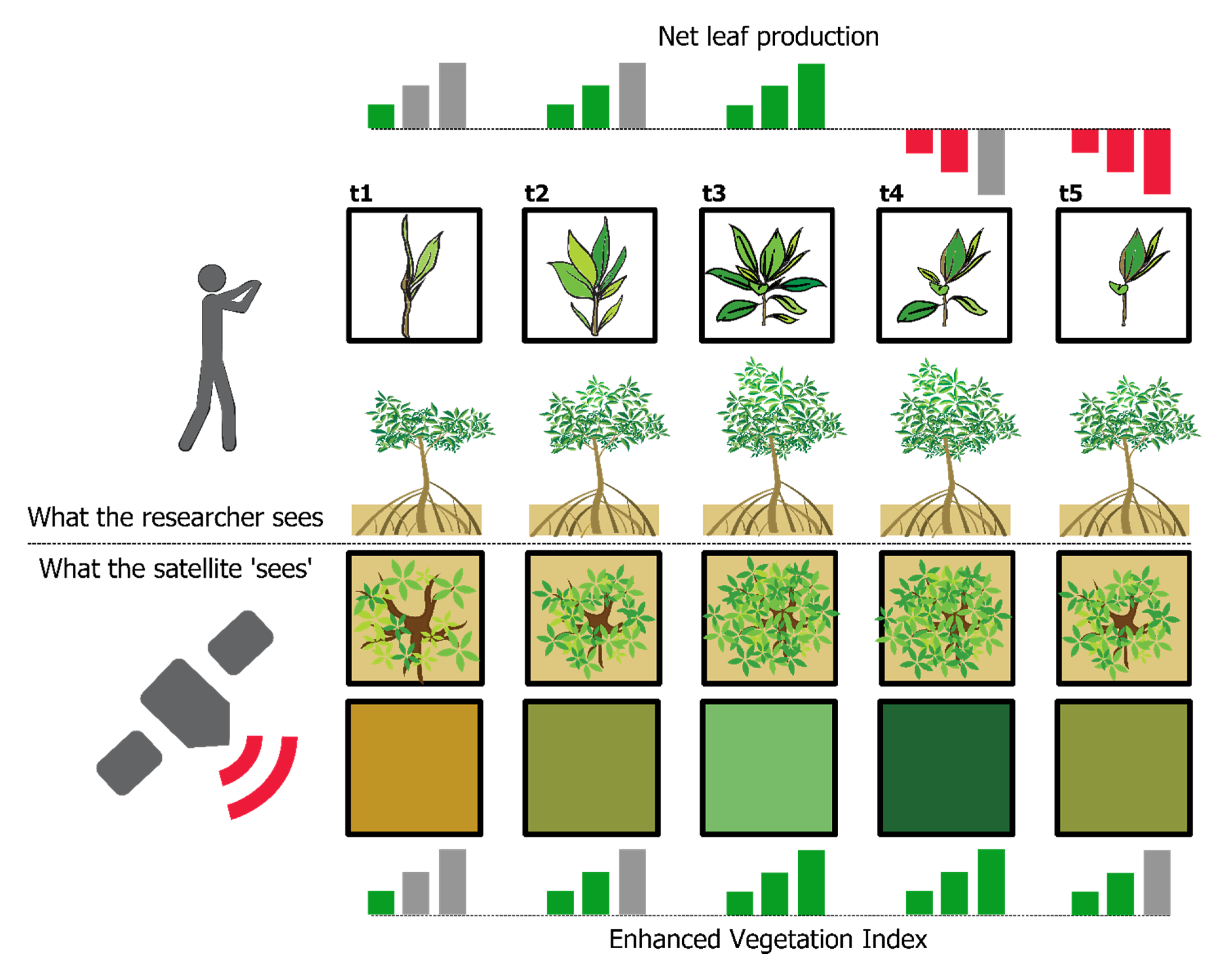
Figure 8 we show an example of this. At “t1”, leaves are scarce and bud breaking, net leaf production and chlorophyll content are low but positive and the satellite captures mainly the background of the mangrove tree (i.e., exposed soil and understory water). At “t2”, leaves are growing and new leaves are bud breaking. At “t3”, net leaf production peaks, meaning that there are many leaves growing and bud breaking, the satellite captures mainly green material, including chlorophyll, thus EVI is high as well. When “t4” arrives EVI is still high, more leaves are dropping than bud breaking, but leaves from “t3” are still growing and reaching maturity (i.e., high chlorophyll content) hence the lag between peak EVI and peak leaf gain/production. Finally, the tree loses more leaves and the background in the satellite images starts to show again (“t5”) and the cycle starts again. The implications of this delayed response of EVI need to be explored because the growth/recovery rate after a natural disaster may not be as evident from satellite imagery as previously thought [
50].
As demonstrated here, GAMs can be used in different locations, and with different species. Single species mangrove ecosystems are rare, and it is common to have a variety of species, especially within a 30 m pixel. Each study site here (
Figure 1) was chosen due to the dominance of
R. stylosa, however, the associated species varied from study to study. From the Northern Territory to the New South Wales coast, our study covers different regions of the Australian coastline and uses data from different points in time, thereby we have demonstrated that GAMs are easily transferable through location and time. As a result, GAMs can be used in local, continental, and global scale models of phenology spanning years or decades. We contribute to the remote sensing community by demonstrating that GAMs can be used in combination with remotely sensed data and presenting an alternative to fully parametric models.
4.4. Moving Forward
Apparent phenology can be detected using a variety of spectral indices, and EVI is only one of several that has been used for coastal ecosystem investigations [
14,
16,
59]. Future studies could use EVI in combination with other spectral indices to improve the detection of phenological events such as accurate measurement of leaf production and different stages of leaf growth. It would also be important to assess whether other spectral indices also display a time lag with relation to net leaf production and whether other phenology models show this temporal shift as well. For example, spectral indices that use the short-wave infra-red region of the spectrum could provide information on water content and indirectly inform the number of leaves in the forest. Establishing this relationship is important, especially in scenarios where mangroves are at risk of massive diebacks such as drought and heatwaves.
Besides temperature, rainfall, and other climate data, other sources of information that can potentially provide additional insights to our model: (1) Fractional Vegetation cover, and (2) radar imagery from Sentinel 1 or Advanced Land Observing Satellite (ALOS) sensors. The use of Radar datasets to monitor mangrove forests has been increasing in the past few years, mainly providing insights on mangrove zonation [
60,
61], canopy structure and height [
62], while Fractional Vegetation Cover informs mangrove dynamics [
13]. The spatial resolution of many of these sensors, including Landsat, does not allow the discrimination of species, however, estimating general trends in mangrove phenology could be more important to protect these forests rather than species-specific values.
We have also identified several ways in which the remote sensing and ecology communities can take phenology modelling to the next level. Firstly, we can evaluate accuracy by gathering and/or sharing field data with sufficient temporal resolution to compare it with satellite imagery. These data could include leaf area index, litterfall, leaf onset, biomass, and other measurements of plant phenology and growth that aid in assessing model accuracy and potential bias. For these efforts to be successful, data collection has to use identical, or at least comparable, techniques to identify and measure the variables of interest. Agreements on how to define and measure mangrove phenology, coupled with high-resolution imagery could greatly benefit this type of studies.
Secondly, GAMs and high-resolution imagery (i.e., equal or better than 1.5 × 1.5 m) can be used to model phenological changes on individual plants. By modelling phenology and the factors that affect it, users can take preventive or corrective measurements before the plant (or crop) fails or dies. More importantly, high-resolution imagery could potentially be used to create models at the same scale as the data collection plots, could be used to monitor restoration projects [
63], and couple phenology to functional traits [
64].
Thirdly, incorporating independent datasets to the GAMs will allow us to examine which environmental variables have the most influence on mangrove phenology at a continental scale. These datasets could include parameters like temperature, rainfall, humidity and tidal range. Besides altering spectral reflectance value values in the near and short-wave infrared bands [
9], the tidal range at the time of image acquisition may play an important role in mangrove phenology. Just like temperature and rainfall, the tides vary seasonally across Australia [
65] and their impact on mangrove phenology is yet to be assessed.
Lastly, we have demonstrated the usefulness of GAMs with a dense time-series of remotely sensed imagery, but the applications of this work could also be used with Moderate-Resolution Imaging Spectroradiometer (MODIS), Sentinel or other satellite sensors. Creating maps of mangroves around the world is important, but we currently have the technology to process large datasets in just hours, so why not model (and forecast) phenology under different climate change scenarios? This means detecting changes in the start of season and peak growing season dates over time and how that may correlate with changing weather and climatic patterns.
5. Conclusions
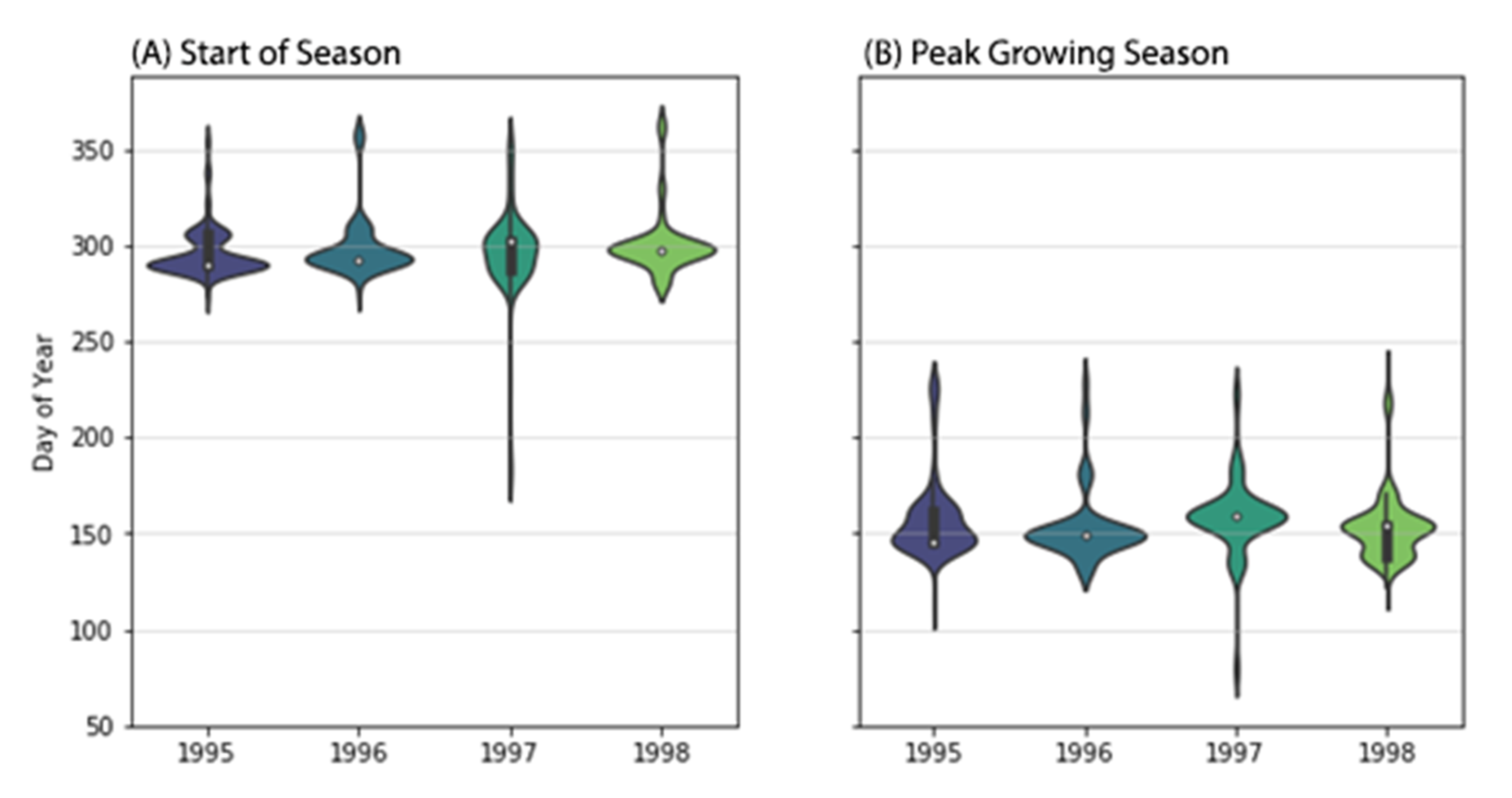
In this paper, we demonstrated that GAMs help us detect (1) the dual phenology of mangrove forests, and (2) seasonal and inter-annual changes in mangrove phenology by using 668 satellite images of different study sites across Australia. The two distinct periods of leaf growth in mangrove forests had not been detected using satellite imager until now. We compared our model to the field and published data to explore which biophysical variables help explain the seasonal changes in EVI. When compared to field data, we found that seasonal and inter-annual variations of EVI correlate well with the leaf production rate, net leaf production of mangrove forests. When compared to published data, we found that there is a time lag between leaf gain and the EVI. Overall, leaf gain and net leaf production are more closely related to higher EVI values than leaf fall. Regarding the phenological metrics, in our Gladstone site, the start of season occurs more frequently between September and October each year and the peak growing season between May and July.
Rather than imposing a parameterized mathematical curve to the data, our study leverages the ability of GAMs to let the data determine the type of relationship between a given spectral index and plant phenology. This data-driven approach helped us detect a bimodal phenology in mangrove forests dominated by R. stylosa; bimodal phenology has been reported in the literature but it has never been seen with remote sensing techniques. More importantly, GAMs allowed us to determine that mangrove phenology is site-dependent. Fully parametric methods, when applied to remotely sensed data, have over-simplified the phenology of mangrove ecosystems and other evergreen forests worldwide.
By understanding how phenology changes from site to site, and year to year, this study provides a tool for regional and continental-scale assessments of mangrove phenology. We expect to see an increase in the use of GAMs, especially in conjunction with the Landsat and other long-term, worldwide imagery archives.

 ,
, 


