Data Fusion Using a Multi-Sensor Sparse-Based Clustering Algorithm

Abstract

The increasing amount of information acquired by imaging sensors in Earth Sciences results in the availability of a multitude of complementary data (e.g., spectral, spatial, elevation) for monitoring of the Earth’s surface. Many studies were devoted to investigating the usage of multi-sensor data sets in the performance of supervised learning-based approaches at various tasks (i.e., classification and regression) while unsupervised learning-based approaches have received less attention. In this paper, we propose a new approach to fuse multiple data sets from imaging sensors using a multi-sensor sparse-based clustering algorithm (Multi-SSC). A technique for the extraction of spatial features (i.e., morphological profiles (MPs) and invariant attribute profiles (IAPs)) is applied to high spatial-resolution data to derive the spatial and contextual information. This information is then fused with spectrally rich data such as multi- or hyperspectral data. In order to fuse multi-sensor data sets a hierarchical sparse subspace clustering approach is employed. More specifically, a lasso-based binary algorithm is used to fuse the spectral and spatial information prior to automatic clustering. The proposed framework ensures that the generated clustering map is smooth and preserves the spatial structures of the scene. In order to evaluate the generalization capability of the proposed approach, we investigate its performance not only on diverse scenes but also on different sensors and data types. The first two data sets are geological data sets, which consist of hyperspectral and RGB data. The third data set is the well-known benchmark Trento data set, including hyperspectral and LiDAR data. Experimental results indicate that this novel multi-sensor clustering algorithm can provide an accurate clustering map compared to the state-of-the-art sparse subspace-based clustering algorithms.

1. Introduction

The recent advances in imaging technology have resulted in the acquisition of high spectral-spatial resolution imaging data [1]. Among the designed imaging sensors, hyperspectral cameras have become the main source of fine spectral-resolution data in hundreds of narrow spectral bands [2]. The spectral channels (bands) of hyperspectral imaging data (HSI) cover the electromagnetic spectrum ranging from the visible to the near-infrared (VNIR, 0.4–1 $\mathsf{\mu }$m) and shortwave infrared (SWIR, 1–2.5 $\mathsf{\mu }$m). An HSI can be employed to identify and discriminate different materials and biological targets [2]. The rich spectral information derived from an HSI has been widely used in remote sensing applications such as land-cover- [3], urban- [4] and mineral-mapping [5,6], or the estimation of above ground biomass [7]. For instance, in the mineral exploration stage, information that is obtained by an HSI can be used as a useful support for geologists to distinguish and track mineralogical features of interest [8].

The analysis of HSI data can be challenging due to (1) their high dimensionality and the often limited availability of representative samples (also known as training samples ), which results in the so-called curse of dimensionality [9] and (2) the highly mixed nature of pixels [10]. In order to overcome these challenges, different machine learning algorithms have been developed and proposed in the last decades [11]. Supervised learning algorithms have become popular for HSI analysis because of their empirical success and adjustability to solve classification and regression problems [12,13]. However, these algorithms strongly rely on training samples, which still remain challenging to obtain.

This issue has been tackled by developing unsupervised algorithms (also known as clustering algorithms) [14]. Clustering algorithms use unlabeled data to group the data into meaningful clusters. Conventional clustering algorithms (e.g., K-means [15], Fuzzy C-means [16]) distribute the data around several cluster centers, the so-called centroids. By using different distance measures, data points are assigned to the cluster with the closest centroid [15]. These clustering algorithms are iterative algorithms and strongly depend on the random initialization of the centroids [17]. Moreover, conventional clustering algorithms are pixel-based, and do not include any spatial information. Additionally, they are only applicable to single-sensor data.

In the past decades, HSIs have been extensively used to detect and characterize different materials, as they provide rich spectral information. At the same time, RGB sensors can generate very detailed high spatial resolution images, while light detection and ranging sensors (LiDAR) can yield geometrical and elevation data [18,19]. All the above-mentioned multi-sensor data sets lead to complementary information (i.e., spectral, spatial, elevation), and the fusion of these data sets has received much attention. In many studies (to name a few [4,5,19,20,21,22,23,24]), the integration of spectral, spatial and elevation information, extracted from multi-sensors has led to significant improvements in the performance of supervised learning-based approaches. In [19], a low-rank subspace-based fusion technique (SubFus) is proposed to incorporate contextual features from multi-sensor data for classification. In [5], the authors proposed to fuse HSI and fine spatial-resolution RGB images using orthogonal total variation component analysis (OTVCA) as a spectral-spatial feature extraction technique. In [21], WorldView 2/3 and LiDAR images were integrated using a deep learning algorithm, the so-called dense convolutional network to map individual tree species in urban areas. A comprehensive review on the integration of multi-sensor and multi-temporal data sets is given in [4].

It has been demonstrated in different studies that high dimensional data can lie in a union of lower dimensional subspaces [14,17,25,26,27,28]. In this way, data points can be grouped into meaningful clusters using subspace information rather than using the complete high dimensional data, and thus reducing the complexity and computational cost [17]. Among the subspace-based clustering algorithms, sparse representation-based algorithms have received much attention in many fields (e.g., feature fusion [29] and image segmentation [14,17,30,31]). The main motivation to use sparsity-based clustering is that the sparse subspace-based clustering algorithm (SSC) was proven to be robust against noise [32]. In addition, the complexity of the optimization with sparse representations is lower than with other representations such as low-rank representations. The sparse subspace clustering method (SSC) is a well-known clustering algorithm, which benefits from the self-expressiveness property. This property states that data points of an HSI can be written as a linear combination of other data points from the same subspace [17]. To solve the SSC optimization problem, the alternative direction method of multipliers (ADMM) is employed. Nevertheless, SSC has some drawbacks: (1) it uses the entire data set for the clustering process, which makes it hard to handle large data sets (this is known as the scalability issue), (2) it only uses spectral information and does not account for the spatial continuity between the data points [14].

During the last decades, several studies have been conducted to cope with the scalability issue. In [33], the authors proposed a landmark-based spectral clustering method (LSC) to handle large data sets. In LSC, spectral clustering is applied on a few representative points (also known as landmark points), which are selected from the data by clustering or random sampling. In [34], a sparse subspace clustering method by using orthogonal matching pursuit (SSC-OMP) was proposed. In [14], an exemplar-based subspace clustering method (ESC) was proposed, which searches for a subset of representative samples, the so-called exemplars that can describe the entire data. Moreover, such an approach allows ESC to reduce the computational cost and to analyze larger data sets. However, the random initialization in search for the exemplars of a data set, results in a less robust performance of ESC. We recently proposed a hierarchical sparse subspace-based clustering (HESSC), as a fast and robust HSI clustering algorithm [28]. In HESSC, the entire data set is explained in different levels of detail using a hierarchical structure, using a lasso-based binary tree and a criterion to split nodes and automatically determine the number of clusters. Nonetheless, all the introduced advanced sparse subspace-based clustering algorithms merely utilize spectral information.

On the other hand, several methods were developed to incorporate spatial information in the sparse subspace-based clustering procedure. In [35], a spatial subspace-based clustering algorithm (SpatSC) was proposed to employ spatial constraints in favor of utilizing information derived from neighboring pixels that have similar features in mineralogical and geological structures. In [26,36], spatial information is exploited by applying a mean or median filter on the computed sparse coefficient matrix in the upgrade phase of ADMM. The above-mentioned algorithms use the entire HSI for clustering, and do not cope with the scalability issue. Additionally, all the mentioned spectral-spatial clustering algorithms use information derived from single-sensor data.

In recent years, several morphological-based algorithms were developed that exploit spatial information for image processing. In [37], for the first time, it was proposed to use morphological profiles (MPs), using opening and closing by reconstruction operators with different structuring elements (SEs) to segment high resolution satellite images. As a follow-up, in [38], extended MPs (EMPs) were introduced as the MPs, which are extracted from the first principle components of an HSI. MPs and EMPs are powerful tools to extract spatial information, but are suffering from a few limitations: (1) the SEs have fixed shapes, (2) they are not suitable to map all the different characteristics of spatial information. In [39], morphological attribute profiles (APs) were proposed to extract structural information of very high resolution images. In APs, morphological attribute filters (i.e., attribute thinning and thickening) are applied on connected components of a gray-scale image to extract different spatial characteristics of a scene. Therefore, APs can be considered as a generalization of MPs that are better able to capture region-based attributes. In order to handle HSIs with APs, extended morphological APs (EMAPs) were proposed [40]. Additionally, in [41,42], different feature extraction techniques (e.g., kernel PCA, multi-linear PCA, and the like) were investigated on the performances of EMPs and EMAPs.

Nevertheless, APs may suffer from an under-segmentation problem, as it may group different regions belonging to several objects. To overcome this problem, invariant attribute profiles (IAPs) were proposed recently [43]. IAPs are built in two phases, the first phase is a spatial invariant feature extraction, where isotropic filtering (by convolutional kernels) is employed to extract the convolutional features of the HSI. This process is followed by a simple linear iterative clustering to spatially aggregate the filtered features. In the second phase, continuous APs are obtained by modeling the variant behaviors of pixels of the HSI. The aforementioned procedure is applied in a Fourier polar coordinate system to avoid discretization artifacts and capture frequency features [44].

In this paper, we propose a spectral-spatial multi-sensor-based clustering algorithm. The proposed algorithm extracts information from both HSI and fine spatial-resolution images. Spectral information is extracted from the HSI, while spatial features (i.e., MPs and IAPs) contain the spatial and elevation information from RGB and LiDAR data. In order to fuse and cluster the obtained information from the different sensors, the concept of HESSC is adopted, in which a fusion between the spectral and spatial features is accomplished at each hierarchical level of the binary tree structure.

The following items summarize the proposed contribution of this paper:

1.

We propose a novel multi-sensor sparse-based clustering algorithm that describes the data at different levels of detail.

2.

To the best of our knowledge, this is the first attempt to incorporate spatial information in the form of morphological-based profiles extracted from multi-sensor data sets in a hierarchical sparse-based clustering algorithm.

3.

In the proposed algorithm, both spectral and spatial features equally contribute at each level of the tree.

4.

The proposed algorithm is able to cluster large-scale data sets.

5.

The proposed algorithm can be adapted to different ancillary remote sensing data sets (e.g., RGB, multi-spectral images, HSI, LiDAR, synthetic aperture radar).

2. Methodology

In this section, we provide a brief overview of the proposed methodology. The workflow of the proposed algorithm is presented in Figure 1. As can be observed from the figure, spatial features are extracted from high-spatial resolution images (i.e., RGB, LiDAR). The process is then followed by establishing a hierarchical (tree) structure to describe the data at various levels of detail. In order to build the tree structure and fuse the spectral and spatial features at the level of the nodes, a lasso-based binary clustering was employed. Finally, if an end-node cannot be divided further, all data points corresponding to this end-node are assigned to one cluster.

2.1. Spatial Feature Extraction

We start to describe the spatial features that are obtained from the auxiliary high spatial-resolution image. As the spatial features, we propose to employ MPs and IAPs, the concepts of which will be described in detail in the following paragraphs.

2.1.1. Morphological Profiles

In [37], extracted MPs rely on two mathematical morphology operators (i.e., opening and closing). These operators are applied on an image with a series of structuring elements (SEs), that can have different shapes (e.g., disc, square, cube) with a user-defined size $r^{\prime }$. With morphological opening, an eroded image is dilated to capture the bright structures in a scene, while with morphological closing, a dilated image is eroded to filter out the dark structures in the scene. Additionally, to preserve the original image structure, a reconstruction filter is applied after the aforementioned morphological operators [41].

Let us assume that $\mathbf{X}={[{\mathbf{x}}_1,{\mathbf{x}}_2,...,{\mathbf{x}}_N]}^T\in {\mathbb{R}}^{b\times N}$ expresses a high spatial-resolution image, where b is the number of spectral channels (e.g., 3 for an RGB image), and N represents the number of pixels in the image. In addition, the location of each pixel in $\mathbf{X}$ is denoted by $(x,y)$ in the Cartesian coordinates. Let ${\gamma }^{SE}\left(\mathbf{X}\right)$ and ${\delta }^{SE}\left(\mathbf{X}\right)$ denote the opening and closing by reconstruction operators on $\mathbf{X}$ with a set of SEs, respectively. In this study, only disk-shaped SEs with variable size are used. MPs are then computed as:

$$\begin{array}{cc}\hfill M{P}_{\gamma }=\{M{P}_{\gamma }^{r^{\prime }}\left(\mathbf{X}\right)=& {\gamma }^{r^{\prime }}\left(\mathbf{X}\right),\forall r^{\prime }\in [0,n]\}\hfill \\ \hfill M{P}_{\delta }=\{M{P}_{\delta }^{r^{\prime }}\left(\mathbf{X}\right)=& {\delta }^{r^{\prime }}\left(\mathbf{X}\right),\forall r^{\prime }\in [0,n]\}\hfill \\ \hfill S.t.{\gamma }^0\left(\mathbf{X}\right)& ={\delta }^0\left(\mathbf{X}\right)=\mathbf{X}\hfill \end{array}$$

(1)

where $r^{\prime }$ is the radius of a disk-shaped SE, and $M{P}_{\gamma }$ and $M{P}_{\delta }$ are the extracted opening and closing MPs by reconstruction [38]; n is a non-negative integer. For more information, we refer to [37,38]. MPs have been widely applied to extract spatial information in remote sensing applications, although they cannot provide all characteristics of the spatial information [11].

2.1.2. Invariant Attribute Profiles

In [43], invariant attribute profiles (IAPs) were defined as the concatenation of two different types of invariant features, i.e., spatial invariant features (SIFs) and frequency invariant features (FIFs).

In order to extract the SIFs, initially, robust convolutional features ${\mathcal{F}}_{RCF}$ are obtained by isotropic filtering of $\mathbf{X}$. For this, each band of the image is convolved with a convolutional kernel in order to aggregate the local spatial information. Then, a simple linear iterative clustering (SLIC), a well-known super-pixel segmentation approach, is applied on $\mathbf{X}$ [45]. Eventually, the extracted convolutional features ${\mathcal{F}}_{RCF}$ are spatially aggregated by the super-pixels. For each pixel i, the SIFs are defined as:

$${\mathcal{F}}_{SIFs}^i=\frac{1}{N_q}\sum _{j=1}^{N_q}{\mathcal{F}}_{RCF}^j,j\in {\varphi }_{i,q}$$

(2)

where ${\varphi }_{i,q}$ is the pixel set of the q-th super-pixel, containing the i-th targeted pixel and a total of $N_q$ pixels.

To derive the frequency invariant features (FIFs), first a polarized Fourier transformation is applied on $\mathbf{X}$. In this way, rotation invariance is obtained by accessing the angular information. From this transformation, three groups of rotation-invariant features are calculated: ${\mathcal{F}}_m^1(x,y)$ are magnitude features corresponding to m different Fourier orders; ${\mathcal{F}}_m^2(x,y)$ are absolute rotation-invariant features, obtained by removing the phase information; ${\mathcal{F}}_m^3(x,y)$ are relative rotation-invariant features, that compensate for the loss of rich phase information. The FIFs are obtained by concatenating these rotation-invariant features and aggregating them into region-based features by using isotropic convolutional filters.

Finally, IAPs are produced by stacking the SIFs and the FIFs: ${\mathcal{F}}_{IAPs}=[{\mathcal{F}}_{SIFs}\cup {\mathcal{F}}_{FIFs}]$. More detailed information on the generation of the IAPs can be found in [43].

2.2. Sparse Subspace Clustering (SSC)

Let $\mathbf{Y}$ denote the input HSI with size $\mathcal{D}\times N$, where $\mathcal{D}$ is the number of spectral bands. ${\mathbf{y}}_i$ represents the ith column vector of $\mathbf{Y}$, where $i\in \{1,2,...,N$} is the pixel index in the HSI, and $y_{ji}$ is the element in row j and column i and denotes band j of that pixel.

The main assumption in sparse subspace clustering methods is that each data point can be described as a linear combination of a dictionary of data points from the same subspace and that all pixels are drawn from a union of L linear subspaces ${\left\{{\mathcal{S}}_l\right\}}_{l=1}^L$ of dimension ${\left\{d_l\right\}}_{l=1}^L$ [17]. Therefore, $\mathbf{Y}$ = $\mathbf{Y}={\mathbf{Y}}_1\cup {\mathbf{Y}}_2\cup {\mathbf{Y}}_3\cup ...\cup {\mathbf{Y}}_L$, where each ${\mathbf{Y}}_l\in {\mathbb{R}}^{\mathcal{D}\times N_l}$ is a sub-matrix of $\mathbf{Y}$, containing $N_l$ pixels from subspace ${\mathcal{S}}_l$. Remark that the number of pixels of each subspace should be larger than the dimension of the subspace ($N_l>d_l$). In most subspace-based clustering algorithms, the number and the dimensions of the subspaces need to be known a priori.

SSC addresses the aforementioned issue by employing the data itself as a dictionary. Accordingly, the following sparse optimization problem is obtained:

$$\begin{array}{cc}\hfill \underset{\mathbf{C}}{arg\; min}{\left|\right|\mathbf{C}\left|\right|}_1& +\frac{\lambda }{2}\left|\right|\mathbf{Y}-{\mathbf{Y}\mathbf{C}\left|\right|}_F^2\hfill \\ \hfill S.t.,& diag\left(\mathbf{C}\right)=\mathbf{0},\hfill \end{array}$$

(3)

where $\mathbf{C}=[{\mathbf{c}}_1,{\mathbf{c}}_2,...,{\mathbf{c}}_N]\in {\mathbb{R}}^{N\times N}$ is the sparse coefficient matrix derived from $\mathbf{Y}$. ${\left|\right|.\left|\right|}_1$ is the ${\ell }_1$-norm: ${\left|\right|\mathbf{C}\left|\right|}_1={\Sigma }_{i=1}^N({\Sigma }_{j=1}^N|c_{ji}\left|\right)$, and ${\left|\right|\mathbf{C}\left|\right|}_F={\Sigma }_{i=1}^N({\Sigma }_{j=1}^N|c_{ji}{{|}^2)}^{\frac{1}{2}}$ represents the Frobenius-norm [17]. $\lambda$ is a trade off parameter between the sparsity and fidelity terms. The constraint $diag\left(\mathbf{C}\right)=\mathbf{0}$ is required to avoid a point being represented as a linear combination of itself. The alternating direction method of multipliers (ADMM) solver is employed to solve the sparse optimization problem of Equation (3) [46]. Consequently, the non-zero elements ($c_{ji}$) of $\mathbf{C}$ identify all data points j that are from the same subspace as i. From $\mathbf{C}$, a symmetrical similarity matrix $\mathbf{W}=\left|\mathbf{C}\right|+{\left|\mathbf{C}\right|}^T$ is obtained, to assure that all pixels from the same subspace are connected to each other.

As the final step, to reduce the dimensionality of the problem, a spectral clustering algorithm [47] is applied on $\mathbf{W}$. For this, the normalized Laplacian matrix is computed: $\mathbf{L}:=\mathbf{D}-\mathbf{W}$, where $\mathbf{D}\in {\mathbb{R}}^{N\times N}$ is a diagonal matrix, with $d_{ii}={\sum }_{j=1}^N{w}_{ij}$. Then, singular-value decomposition (SVD) is applied on $\mathbf{L}$, to obtain the eigenvectors $\mathbf{V}\in {\mathbb{R}}^{N\times A}$, corresponding to the A smallest non-zero eigenvalues of $\mathbf{L}$. Finally, clustering (we used K-means clustering) is applied on $\mathbf{V}$ to generate the clustering map [17,47].

The main advantage of SSC is that the clustering is applied on the similarity matrix of the sparse coefficient matrix, rather than directly on the data. In this way, the subspace structure of the data is accounted for, and makes the clustering more robust to the initialization compared to the conventional clustering algorithms (e.g., K-means, FCM) [48].

Although SSC performs well to cluster HSIs, it also has shortcomings. SSC has a scalability issue, in which it requires to use all data points to solve the optimization problem in Equation (3), which can be computationally expensive in the case of large data sets. Another shortcoming of SSC is that the algorithm only uses spectral information and does not take into account the spatial context of the HSI.

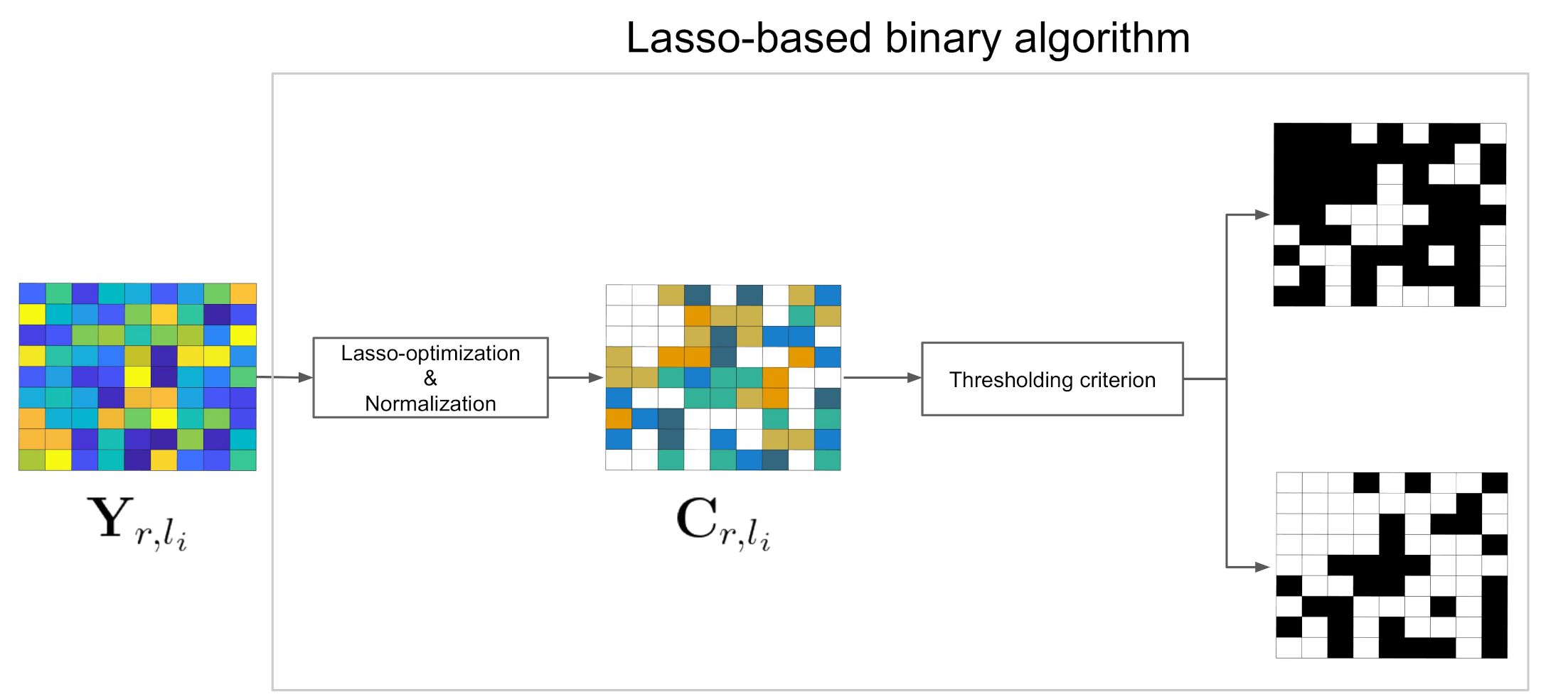
2.3. Hierarchical Sparse Subspace Clustering (HESSC)

Several sparse subspace-based clustering algorithms have been proposed in order to tackle the scalability issue, [14,27,28,49]. In our earlier work [28], we proposed an automatic hierarchical sparse subspace-based clustering (HESSC) algorithm to analyze HSIs. HESSC is able to describe an HSI at different hierarchical levels in a robust and automatic manner by employing a binary tree structure.

Starting from all data points in the HSI, at each level, nodes are split into two groups. Let us denote ${\mathbf{Y}}_{l_i}$ as the collection of all the data points in one of the parental nodes at level $l_i$. Then, ${\mathbf{Y}}_{l_i}={\cup }_{r=1}^2{\mathbf{Y}}_{r,l_{i+1}}$, where ${\mathbf{Y}}_{r,l_{i+1}}$ denote the collection of all data points in each of the two child nodes at level $i+1$. The criterion to split the nodes is based on the generation of a binary matrix, obtained by the following sparse optimization problem:

$$\underset{{\mathbf{C}}_{l_i}}{arg\; min}\left|\right|{\mathbf{C}}_{l_i}{\left|\right|}_1+\frac{\lambda }{2}\left|\right|{\mathbf{Y}}_{l_i}-{\mathbf{y}}_j{\mathbf{C}}_{l_i}{\left|\right|}_F^2,$$

(4)

where ${\mathbf{C}}_{l_i}$ is the computed sparse coefficients derived from ${\mathbf{Y}}_{l_i}$, and ${\mathbf{y}}_j$ is the j-th column vector of ${\mathbf{Y}}_{l_i}$, where j is randomly selected. To solve the above optimization problem, the lasso version of the least angle regression algorithm is used [50]. Subsequently, the computed ${\mathbf{C}}_{l_i}$ is normalized, and thresholded (with a user-defined threshold) to generate a binary matrix (BM) (Figure 2). In order to assure the robustness of HESSC, the aforementioned procedure is repeated 100 times, with randomly selected ${\mathbf{y}}_j$, each time generating a binary matrix. Subsequently, the generated BMs are fed to an entropy-based consensus clustering algorithm (ECC) [51] to produce the final binary matrix that eventually splits the current node into two child nodes.

A stopping criterion is applied to decide whether a node should be further split. The stopping criterion is either manual, when the required number of clusters is known prior and pre-defined by the user, or automatic, based on a Singular Value Decomposition of the data [52]. When a node is not split any further, its’ corresponding data points are labeled as one cluster.

Although HESSC is able to cluster an HSI in a robust and fast manner, only spectral information is utilized. In this work, we will extend HESSC to include spatial information that is derived from high spatial-resolution data from the same scene as the HSI.

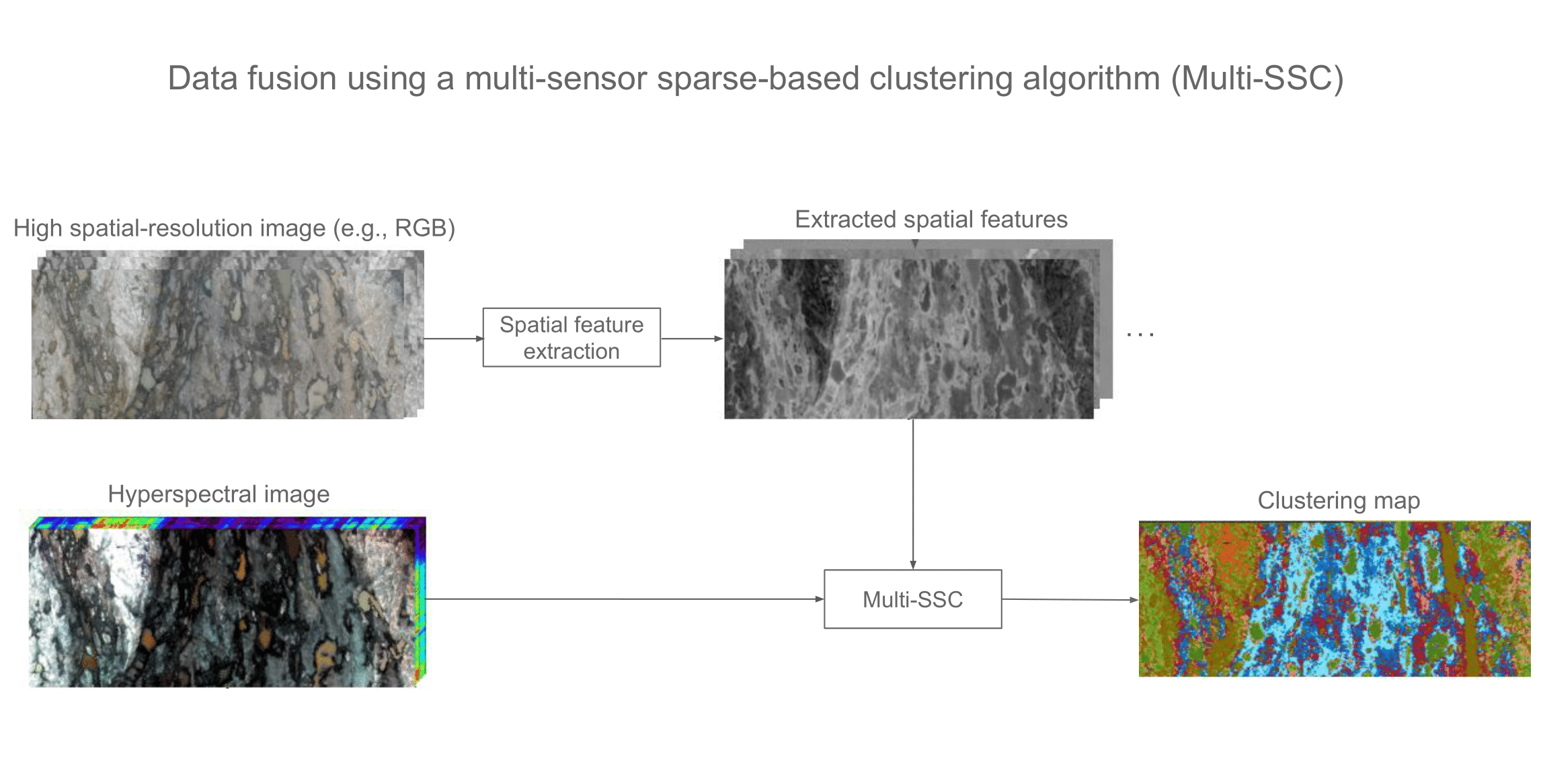
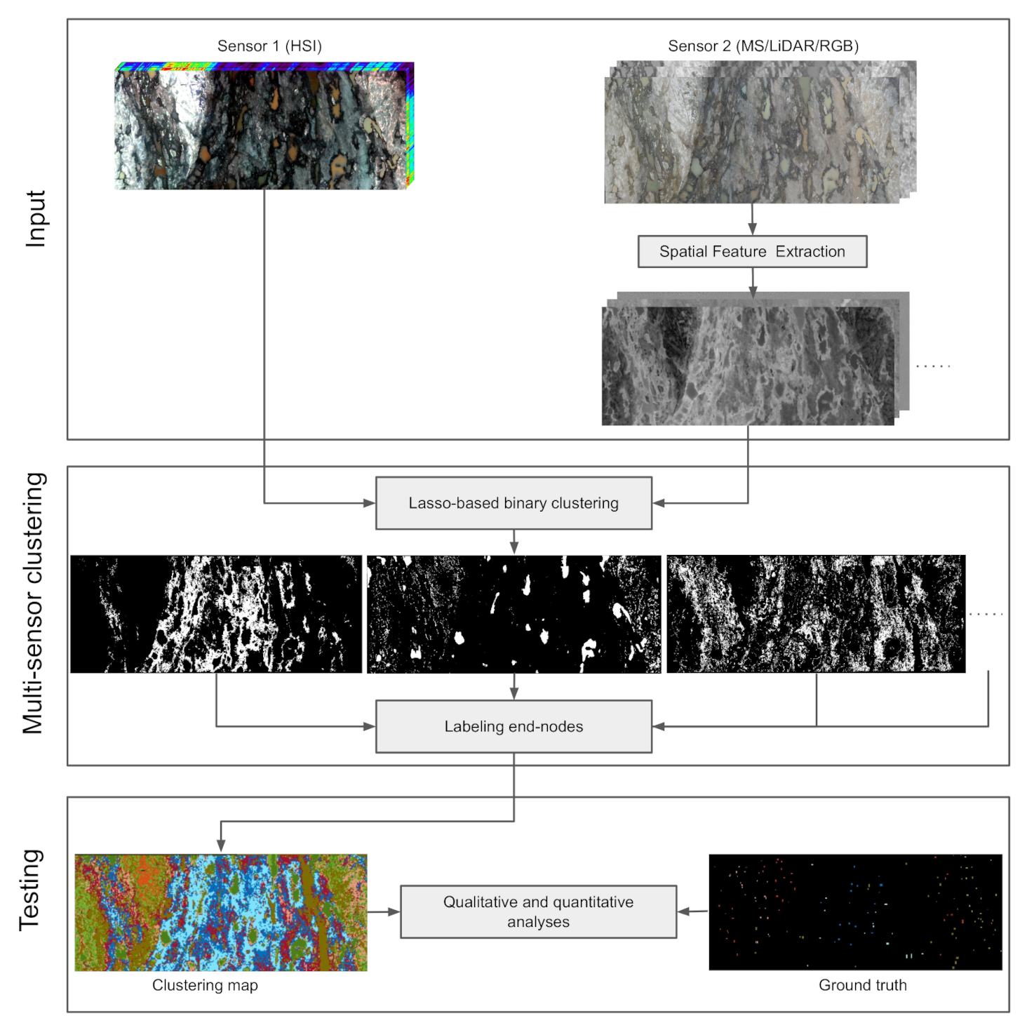
2.4. Multi-Sensor Spectral-Spatial Sparse-Based Clustering (Multi-SSC)

One way of fusing spectral and spatial information is to extract spatial features from an HSI, and combining (e.g., concatenating) the extracted spatial features with the spectral channels [53]. However, such a single-sensor integration approach might not contain sufficient spatial and contextual information. We therefore propose to explicitly incorporate the spatial information derived from high spatial-resolution data sets (i.e., high spatial-resolution RGB and LiDAR images) [19].

In the proposed Multi-SSC, a hierarchical tree approach, similar to the HESSC algorithm is used. However, at each level of the binary tree, a parental node is split, based on binary matrices, each of which is generated from either spectral or spatial information. To generate a BM from spectral information, the sparse optimization problem of Equation (4) is solved and the obtained sparse coefficient matrix is thresholded. To generate a BM from spatial information, the following sparse optimization problem is defined:

$$\underset{{\mathbf{C}}_{l_i}}{arg\; min}\left|\right|{\mathbf{C}}_{l_i}{\left|\right|}_1+\frac{\lambda }{2}\left|\right|{\mathcal{F}}_{SF{E}_{l_i}}-{\mathcal{F}}_{SF{E}_j}{\mathbf{C}}_{r,l_i}{\left|\right|}_F^2,$$

(5)

where ${\mathcal{F}}_{SF{E}_{l_i}}$ denotes the extracted spatial features (either MPs or IAPs) from all data points at the specific parental node of level $l_i$. ${\mathcal{F}}_{SF{E}_j}$ is the j-th column vector of ${\mathcal{F}}_{SF{E}_{l_i}}$, which has been randomly selected. The obtained sparse coefficient matrix is then thresholded to generate the BM.

To cope with uncertainties of the model [54] that may be introduced by the random selection of both ${\mathcal{F}}_{SF{E}_j}$ and ${\mathbf{y}}_j$, we apply the ECC algorithm [51]. Additionally, to include both spectral and spatial information in a balanced way, an equal number of BMs are generated from the optimizations of Equations (4) and (5). Depending on the specific application, this ratio can be adapted. In this work, we choose to apply each of the optimizations 50 times. The total of 100 BMs are then processed by the ECC algorithm to produce the final binary matrix, which is used for the further division of the current node. The stopping criterion is the same as applied in Section 2.3. The final clustering map is generated by labeling the nodes of the tree, which are not further split.

3. Experiments

3.1. Data Acquisition and Description

In order to evaluate the generalization capability of the proposed method, we take into account two important factors for the selection of data sets: (1) the investigated data sets cover different scene types (i.e., geological and rural areas) and (2) different sensor combinations and types are investigated (i.e., HSI, RGB, and LiDAR). For this reason, we chose the following data sets:

(1)

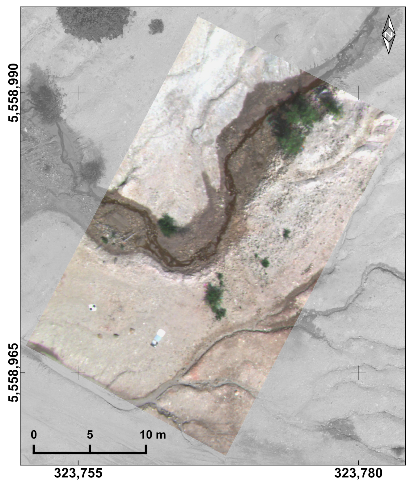
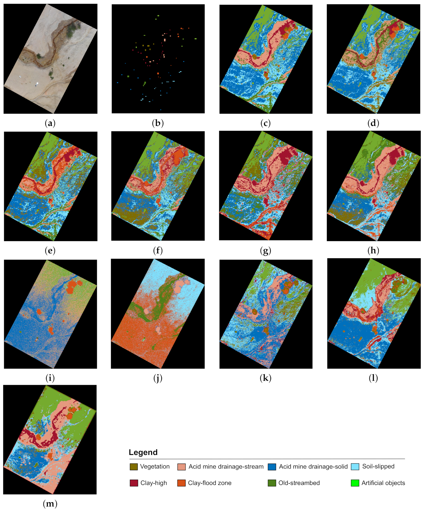
Czech data : The first data set was acquired near the Litov tailing lake and its adjacent waste heap, situated in the Sokolov district of the Czech Republic. Both HSI and RGB images were acquired. The HSI was acquired by a hyperspectral frame-based camera (0.6 Mp Rikola Hyperspectral Imager), which was deployed on a hexacopter unmanned aerial vehicle (UAV; Aibotix Aibot X6v2) along with a pre-programmed stop-scan-motion flight plan to capture a complete set of HSIs for the subsequent image mosaicking. The RGB image was captured by employing a senseFly S.O.D.A. RGB camera, deployed on a fixed-wing UAV. The spatial resolution of the captured RGB image is 1.5 cm. It is downsampled to the size of the HSI data ($1066\times 909$ pixels), which has a spatial resolution of 3.3 cm and is composed of 50 spectral bands ranging from 0.50–0.90 $\mathsf{\mu }$m. Figure 3 illustrates the acquired RGB image of the Czech data set.

(2)

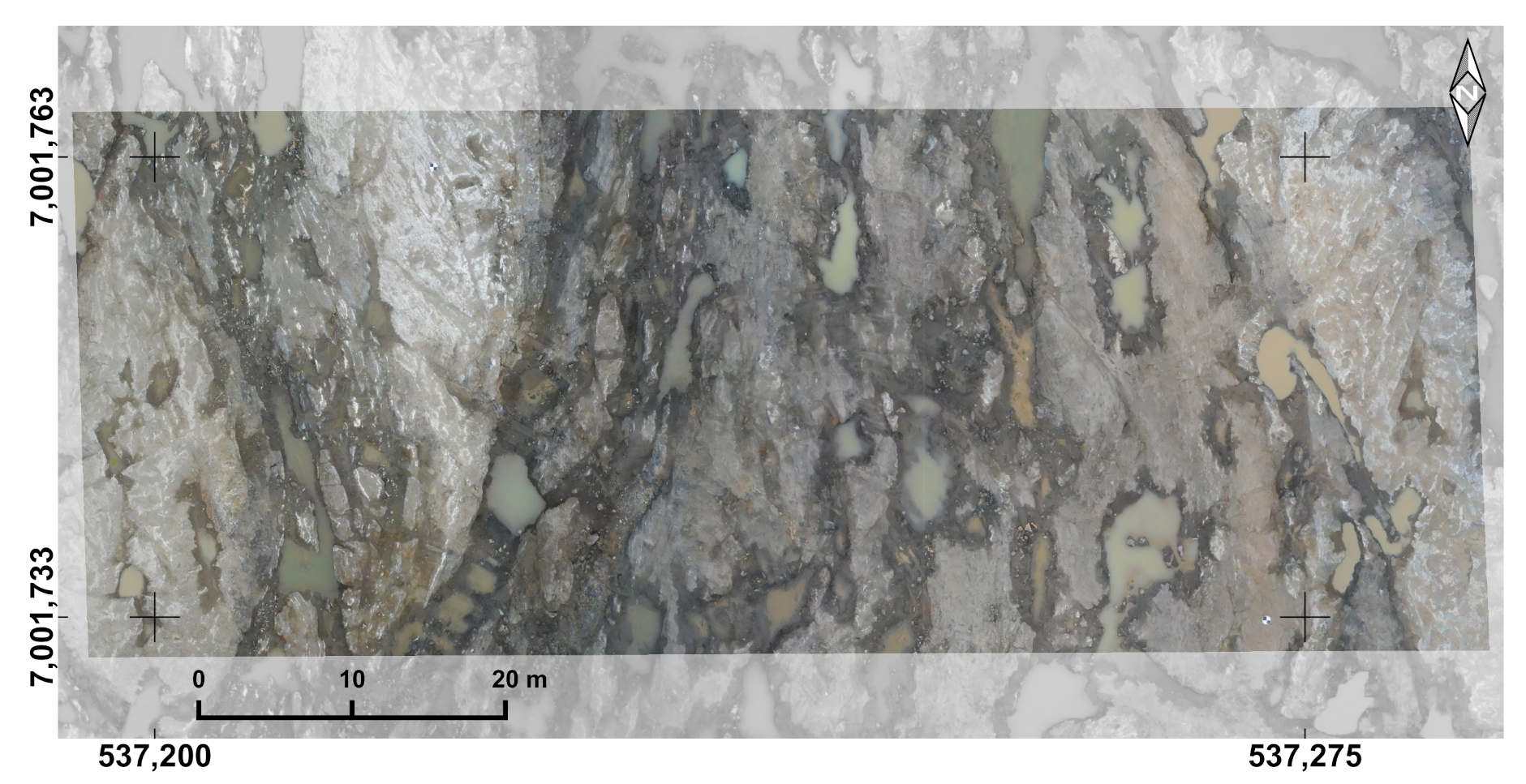
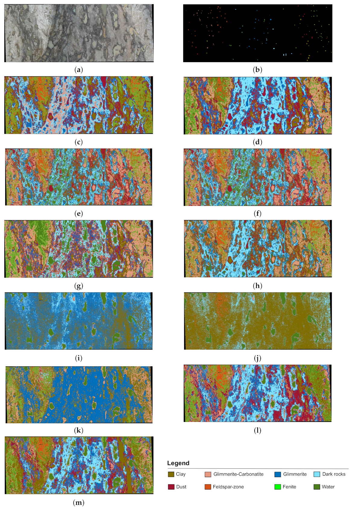
Finland data: The second data set was captured over an outcrop of the Archean Siilinjärvi glimmerite-carbonatite complex in Finland, which is currently mined for large phosphate-rich apatite occurrences used in fertilizer production [55]. In the Finland data set, the same instruments were employed to acquire the HSI and RGB data. The HSI and downsampled RGB images are composed of $718\times 1848$ pixels. Figure 4 displays the acquired RGB image of the Finland data set.

(3)

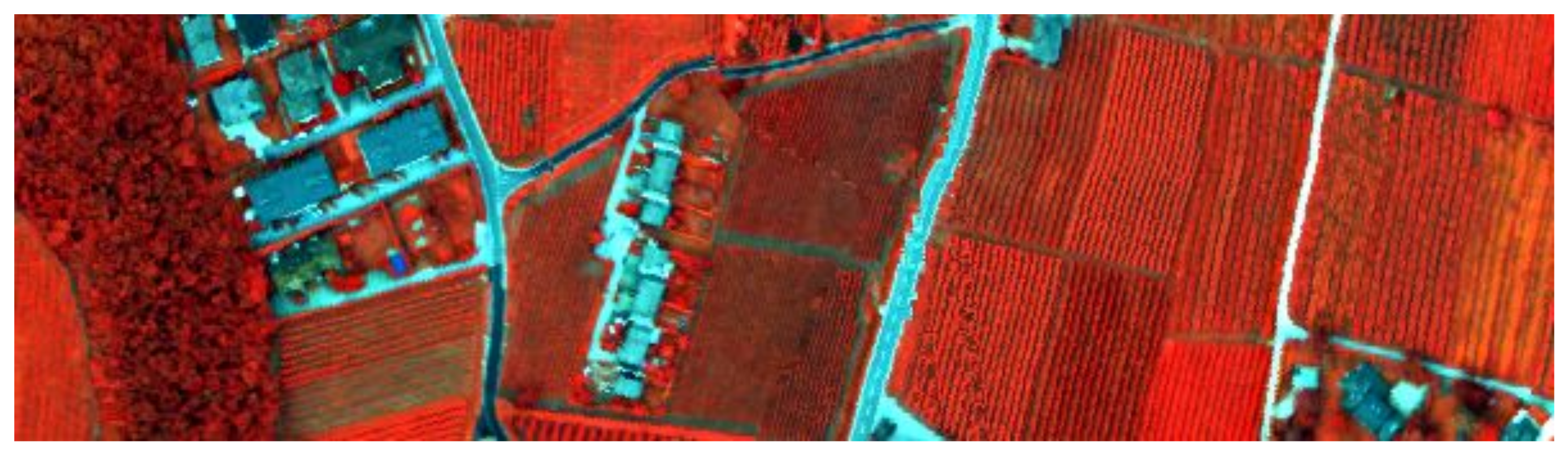
Trento data: The third data set was captured over a rural area in the south of the city of Trento, Italy. It consists of LiDAR and HSI data that are composed of 600 by 166 pixels with a spatial sampling of 1 m. The HSI was acquired by the AISA Eagle sensor, and contains 63 spectral bands ranging between 0.40 and 0.98 $\mathsf{\mu }$m. The LiDAR data were captured by the Optech ALTM 3100EA sensor. The color-composite image of the HSI from the Trento data is shown in Figure 5.

For the fusion procedure, the co-registered high-spatial resolution RGB/LiDAR images have already been downsampled to their corresponding HSIs. In the case of geological data sets, the resampling was carried out by using the nearest-neighborhood method in Quantum GIS (version 3.4, QGIS development team, Open Source Geospatial Foundation). The internal image co-registration of hyperspectral scans was done by registering all bands on a distinct master band per hypercube, using the MEPHySTo image processing toolbox [56], used for pre-processing of the hypercubes. Georeferencing of all images was done on high-resolution drone-based RGB orthophotos, created by structure-from-motion photogrammetry in Agisoft Photoscan (version 1.4, Agisoft LLC, St. Petersburg, Russia). The UAV-based, GPS-tagged Orthophotos were acquired over the target area and their positioning was refined by using ground control points. Further data acquisition details for the Czech data set are referenced in [57], and for the Finland data set in [58].

3.2. Experimental Setup

Quantitative and qualitative analyses were conducted to evaluate the performance of our proposed algorithm. The clustering results obtained by Multi-SSC with MPs and IAPs were compared with the results of two conventional clustering algorithms K-means and FCM, along with the scalable clustering algorithms, LSC [33], ESC [14], and HESSC [28]. Additionally, to allow a fair comparison, the concatenation of the HSI and RGB/LiDAR images (e.g., the combination of HSI and RGB has $\mathcal{D}+3$ features) is fed into all of the applied clustering algorithms to evaluate their performances. Moreover, to assess the effect of extracted IAPs on the clustering performance, IAPs are stacked with the spectral bands of the HSI and used as the input for the competitive clustering algorithms. For the remaining, the following acronyms are used: $A{L}_{sensor}$, where $AL$ is the name of the applied clustering algorithm and $sensor$ refers to the applied data (HSI is only spectral data, HSI+RGB and HSI+LiDAR representing the concatenation of spectral bands and RGB/LiDAR bands, HSI+IAPs denotes the concatenation of spectral bands and IAPs).

All utilized parameters in ESC were set as the default parameters proposed by the developers [14]. In LSC, the K-means sampling strategy was used to produce the landmark points. In HESSC, the threshold $\tau$ in the lasso-based binary was set to $0.5$, the default by the developers [28]. For the MPs, suitable radii $r^{\prime }$ for the SEs were selected for the first and second data sets by visual inspection. In the first data set, $r^{\prime }=[1,5,10,15,20,40,60,80,100]$ were chosen. In the second data set, $r^{\prime }=[10,20,40,60,80,100]$, and for the last data set, $r^{\prime }=[10,20,40,60]$ were used, as in [19]. Regarding the parameters used in extracting the IAPs, we followed the same setup as suggested by the developers in [43], where the number of scaled convolutions and their radii were set to 3 and [2,4,6], respectively. The Fourier orders to derive the frequency features were set to $m=[0,1,2]$, and for all data sets, we used the first three principal components to generate the IAPs.

All quantitative results are reported as an average of 10 runs. All the applied algorithms in this study were implemented in MATLAB version 2019b on a computer with an Intel© core-i9 7900X with 128 GB RAM.

3.3. Evaluation Metrics

Three commonly used evaluation metrics are employed: overall accuracy (OA), average accuracy (AA), and kappa coefficient ($\kappa$). The ground truth data set is represented by $\mathbf{G}=[g_1,g_2,...,g_N]$. The clustering result can be presented as $\mathbf{M}=[m_1,m_2,...,m_N]$, where $m_i=1,...,\mathcal{L}$, the index of the class label, assigned to each pixel. To assess the clustering performance, $m_i$ needs to be matched with $g_i$. We thus employed $m_i^{\prime }=bestMap(g_i,m_i)$ as a matching function, based on the Hungarian algorithm, where $m_i^{\prime }$ is the clustering map for which the best match between $g_i$ and $m_i$ is produced by $bestMap(.)$ [59]. Consequently, OA is defined as ${\Sigma }_{i=1}^N\Gamma (m_i^{\prime },g_i)/N$, where $\Gamma (m_i^{\prime },g_i)$ is 1 if $g_i=m_i^{\prime }$ and 0 otherwise.

In addition to the three aforementioned metrics, two generally applied clustering indices are employed:

(1) The adjusted rand index (ARI) is used as a similarity (or dissimilarity) measure between two partitions and it is an adjusted version of the original rand index [60]. According to [60], ARI can be formulated as:

$$\frac{{\sum }_{ij}\left(\genfrac{}{}{0pt}{}{n_{ij}}{2}\right)-{\sum }_i\left(\genfrac{}{}{0pt}{}{n_{i+}}{2}\right){\sum }_j\left(\genfrac{}{}{0pt}{}{n_{+j}}{2}\right)/\left(\genfrac{}{}{0pt}{}{n}{2}\right)}{\frac{1}{2}[{\sum }_i\left(\genfrac{}{}{0pt}{}{n_{i+}}{2}\right)+{\sum }_j\left(\genfrac{}{}{0pt}{}{n_{+j}}{2}\right)]-{\sum }_i\left(\genfrac{}{}{0pt}{}{n_{i+}}{2}\right){\sum }_j\left(\genfrac{}{}{0pt}{}{n_{+j}}{2}\right)/\left(\genfrac{}{}{0pt}{}{n}{2}\right)}$$

(6)

where, $n_{ij}=|m_i^{\prime }\cap g_j|$, $n_{i+}$ and $n_{+j}$ are equal to ${\sum }_{j=1}^N{n}_{ij}$ and ${\sum }_{i=1}^N{n}_{ij}$, respectively. The range of ARI is usually between 0 and 1. An ARI closer to one means that $\mathbf{M}$ and $\mathbf{G}$ highly agree. However, it is also possible that the ARI becomes negative, indicating that the agreement between $\mathbf{M}$ and $\mathbf{G}$ is even less than what is expected from a random result.

(2) The normalized mutual information (NMI) is calculated based on the mutual information between $\mathbf{M}$ and $\mathbf{G}$. The mutual information is normalized to range NMI between 0 and 1 [61]. NMI can be calculated as:

$$\frac{{\sum }_{ij}{n}_{ij}log\frac{n_i{n}_{ij}}{n_{i+}{n}_{+j}}}{\sqrt{({\sum }_i{n}_{i+}log\frac{n_{i+}}{n})({\sum }_j{n}_{+j}log\frac{n_{+j}}{n})}}$$

(7)

Similar to ARI, the agreement between $\mathbf{M}$ and $\mathbf{G}$ is higher when NMI is closer to 1.

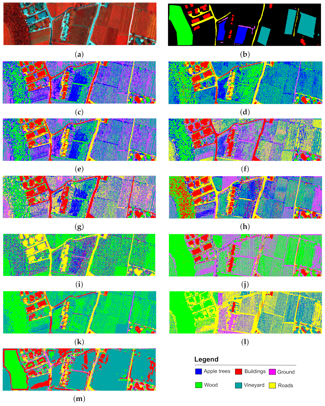
3.4. Results and Discussion

Results of all experiments are summarized in

Table 1. Quantitative assessment of the performances of the clustering algorithms applied to the Czech data. The clustering accuracy is reported using OA, AA, $\kappa$, ARI, and NMI. In addition, the processing time is reported as well.

Class	No. Ground Truth Samples	K-means${}_{\mathit{HSI}}$	K-means${}_{\mathit{HSI}+\mathit{RGB}}$	K-means${}_{\mathit{HSI}+\mathit{IAPs}}$	FCM${}_{\mathit{HSI}}$	FCM${}_{\mathit{HSI}+\mathit{RGB}}$	FCM${}_{\mathit{HSI}+\mathit{IAPs}}$	LSC${}_{\mathit{HSI}}$	LSC${}_{\mathit{HSI}+\mathit{RGB}}$	LSC${}_{\mathit{HSI}+\mathit{IAPs}}$	ESC${}_{\mathit{HSI}}$	ESC${}_{\mathit{HSI}+\mathit{RGB}}$	ESC${}_{\mathit{HSI}+\mathit{IAPs}}$	HESSC${}_{\mathit{HSI}}$	HESSC${}_{\mathit{HSI}+\mathit{IAPs}}$	Multi-SSC (MPs)	Multi-SSC (IAPs)
1	1018	50.49	87.92	91.06	36.05	84.87	44.40	100	93.42	80.35	100	99.71	98.04	63.06	89.00	55.50	97.05
2	901	98.67	93.01	88.67	97.34	10.54	66.89	0.00	0.11	99.00	99.00	99.67	53.50	66.26	26.53	77.36	99.67
3	1119	73.73	71.40	71.94	63.81	71.67	46.85	50.67	79.54	67.74	41.82	0.54	41.82	22.88	0.00	51.03	36.73
4	874	52.86	0.00	3.43	65.90	29.18	60.64	64.30	16.82	65.22	0.57	2.17	94.16	47.94	86.61	80.32	56.86
5	838	97.61	99.05	87.61	96.06	98.69	86.42	95.94	97.02	0.12	41.77	80.19	0.00	65.75	68.50	56.44	85.68
6	863	31.29	66.74	68.25	58.86	42.53	59.10	35.57	42.41	47.74	0.12	86.33	0.00	12.05	98.73	86.79	29.66
7	777	38.74	49.55	35.39	35.91	46.72	35.65	35.39	55.08	33.33	10.29	0.00	11.45	65.89	16.22	28.06	32.95
8	785	0.00	7.39	31.97	4.59	2.55	4.59	8.54	19.75	9.94	43.95	51.72	79.36	43.82	38.85	17.71	80.13
OA		56.85	61.06	61.37	58.00	50.08	56.70	50.17	52.28	55.68	43.05	52.42	45.45	47.74	52.13	57.34	64.85
AA		55.42	59.38	59.79	57.31	48.34	50.57	48.80	50.51	50.43	42.19	52.54	47.29	48.45	53.05	56.65	64.84
$\kappa$		0.50	0.55	0.58	0.51	0.42	0.48	0.42	0.45	0.45	0.34	0.45	0.48	0.40	0.46	0.51	0.59
$ARI$		0.50	0.47	0.49	0.41	0.42	0.36	0.37	0.45	0.33	0.22	0.36	0.53	0.31	0.35	0.53	0.54
$NMI$		0.63	0.62	0.63	0.54	0.56	0.51	0.53	0.58	0.51	0.41	0.55	0.62	0.50	0.52	0.64	0.66
t (seconds)		1.16	1.01	1.66	145.12	187.09	196.62	34.65	34.94	35.01	13,387.00	9859.00	11,130.00	3562.80	3557.20	3086.51	3114.80

,

Table 2. Quantitative assessment of the performances of the clustering algorithms applied to the Finland data. The clustering accuracy is reported using OA, AA, $\kappa$, ARI, and NMI. In addition, the processing time is reported as well.

Class	No. Ground Truth Samples	K-means${}_{\mathit{HSI}}$	K-means${}_{\mathit{HSI}+\mathit{RGB}}$	K-means${}_{\mathit{HSI}+\mathit{IAPs}}$	FCM${}_{\mathit{HSI}}$	FCM${}_{\mathit{HSI}+\mathit{RGB}}$	FCM${}_{\mathit{HSI}+\mathit{IAPs}}$	LSC${}_{\mathit{HSI}}$	LSC${}_{\mathit{HSI}+\mathit{RGB}}$	LSC${}_{\mathit{HSI}+\mathit{IAPs}}$	ESC${}_{\mathit{HSI}}$	ESC${}_{\mathit{HSI}+\mathit{RGB}}$	ESC${}_{\mathit{HSI}+\mathit{IAPs}}$	HESSC${}_{\mathit{HSI}}$	HESSC${}_{\mathit{HSI}+\mathit{IAPs}}$	Multi-SSC (MPs)	Multi-SSC (IAPs)
1	1062	53.58	54.43	71.28	48.96	49.81	66.20	68.17	50.85	31.17	77.78	95.67	13.75	54.90	75.33	56.97	100
2	791	0.00	25.92	20.86	0.00	0.00	0.00	3.92	1.64	9.99	1.39	1.90	41.09	22.12	4.23	8.34	2.28
3	1048	54.48	65.55	61.45	31.58	32.44	55.15	41.70	37.40	52.86	71.28	0.00	7.63	0.00	89.50	53.34	71.18
4	994	50.80	94.16	55.33	43.86	44.47	52.11	47.38	56.94	66.90	0.00	0.80	0.00	96.38	24.14	85.92	85.01
5	964	56.64	45.33	65.66	61.51	62.14	68.67	40.87	39.63	43.57	1.04	0.00	45.75	0.21	7.57	3.01	12.34
6	1061	88.22	69.18	87.75	86.90	86.71	88.03	0.00	89.44	94.25	0.19	30.73	26.86	42.79	82.75	83.69	71.25
7	1065	35.87	58.59	0.00	37.84	38.12	11.87	70.05	30.42	16.42	34.46	37.46	94.96	57.46	15.83	98.22	56.81
8	1011	0.00	10.29	68.83	37.29	38.67	57.28	85.66	29.28	37.93	100	100	19.15	88.82	33.71	49.11	91.10
OA		43.88	53.84	53.15	44.80	45.36	51.62	45.89	43.30	44.68	37.19	34.70	40.71	46.05	44.56	56.49	63.43
AA		42.45	52.93	53.90	43.49	44.05	49.91	44.72	41.95	44.14	35.77	33.32	31.15	45.34	41.63	54.82	61.25
$\kappa$		0.35	0.47	0.48	0.36	0.37	0.44	0.38	0.35	0.37	0.27	0.24	0.21	0.38	0.42	0.50	0.58
$ARI$		0.27	0.38	0.32	0.28	0.27	0.36	0.30	0.27	0.33	0.16	0.11	0.28	0.34	0.23	0.41	0.46
$NMI$		0.42	0.52	0.49	0.43	0.42	0.51	0.49	0.42	0.51	0.37	0.35	0.38	0.51	0.42	0.55	0.57
t (seconds)		27.81	54.56	55.45	318.40	339.15	338.18	52.05	57.71	71.11	100,890.00	100,210.00	110,700.00	12,085.00	70,492.00	90,436.00	98,752.00

and

Table 3. Quantitative assessment of the performances of the clustering algorithms applied to the Trento data. The clustering accuracy is reported using OA, AA, $\kappa$, ARI, and NMI. In addition, the processing time is reported as well.

Clusters	No. Ground Truth Samples	K-means${}_{\mathit{HSI}}$	K-means${}_{\mathit{HSI}+\mathit{LiDAR}}$	K-means${}_{\mathit{HSI}+\mathit{IAPs}}$	FCM${}_{\mathit{HSI}}$	FCM${}_{\mathit{HSI}+\mathit{LiDAR}}$	FCM${}_{\mathit{HSI}+\mathit{IAPs}}$	LSC${}_{\mathit{HSI}}$	LSC${}_{\mathit{HSI}+\mathit{LiDAR}}$	LSC${}_{\mathit{HSI}+\mathit{IAPs}}$	ESC${}_{\mathit{HSI}}$	ESC${}_{\mathit{HSI}+\mathit{LiDAR}}$	ESC${}_{\mathit{HSI}+\mathit{IAPs}}$	HESSC${}_{\mathit{HSI}}$	HESSC${}_{\mathit{HSI}+\mathit{IAPs}}$	Multi-SSC (MPs)	Multi-SSC (IAPs)
1	4034	70.91	38.34	59.67	75.90	24.86	55.35	60.13	43.27	55.33	10.55	26.82	2.78	0.00	45.70	29.30	0.00
2	2903	89.25	98.97	0.55	84.46	99.44	0.65	0.00	35.59	2.17	10.08	99.22	64.17	80.26	81.46	36.33	68.55
3	479	0.00	15.64	30.90	59.46	59.67	32.36	10.77	16.16	24.84	42.78	4.13	63.67	21.71	25.65	9.60	26.72
4	9123	57.07	86.35	99.93	0.00	69.86	99.91	56.70	68.82	99.62	34.35	74.15	54.58	91.69	70.65	99.95	90.57
5	10,501	42.79	48.68	69.05	39.18	22.42	68.50	35.81	36.88	60.01	69.37	44.05	73.32	43.70	39.11	59.26	94.47
6	3174	31.23	15.72	52.96	53.09	7.63	53.02	94.72	90.65	70.01	83.81	46.84	50.50	55.45	34.00	82.89	44.83
OA		51.97	59.52	63.22	53.88	54.21	58.65	47.71	52.96	63.76	46.34	63.95	54.13	56.76	52.09	65.12	71.90
AA		48.54	50.61	52.18	51.18	44.77	51.63	43.02	49.23	52.00	41.82	49.20	51.50	48.80	49.43	52.89	54.19
$\kappa$		0.46	0.46	0.53	0.43	0.42	0.54	0.37	0.45	0.54	0.27	0.50	0.51	0.41	0.49	0.55	0.61
$ARI$		0.27	0.16	0.50	0.28	0.16	0.51	0.28	0.18	0.42	0.21	0.30	0.32	0.37	0.36	0.44	0.53
$NMI$		0.43	0.25	0.54	0.46	0.25	0.54	0.45	0.26	0.56	0.37	0.44	0.38	0.49	0.46	0.58	0.64
t (seconds)		2.55	2.73	3.01	21.69	20.42	11.60	3.86	2.48	2.96	763.52	118.92	764.79	478.94	576.11	407.49	518.63

, for the Czech, Finland and Trento data, respectively.

3.4.1. The Czech Data Set

The Czech data set contains 8 classes: (1) Vegetation, (2) Acid mine drainage-stream, (3) Acid mine drainage-solid, (4) Soil-slipped, (5) Clay-high, (6) Clay-flood zone, (7) Old-stream bed and (8) Artificial objects.

Table 1 summarizes all clustering results. The proposed method outperforms all other clustering approaches. The clustering performance of HESSC${}_{HSI}$ is weak, when compared to K-means${}_{HSI}$, FCM${}_{HSI}$, and LSC${}_{HSI}$, which may be due to the high similarity between the spectral signatures of the different classes. The concatenation of extracted IAPs improves the accuracy of HESSC${}_{HSI+IAPs}$ with 5% over HESSC${}_{HSI}$. Another 12% improvement is observed when fusing the spectral and IAPs in the proposed approach Multi-SSC, when compared to concatenating them in HESSC${}_{HSI+IAPs}$. With respect to the clustering results of individual classes, one can observe that class 2 and 8 are accurately mapped using Multi-SSC (IAPs), while class 4 and 6 are better mapped using Multi-SSC (MPs). ESC${}_{HSI+RGB}$ is able to capture class 2 perfectly, while both versions of LSC perform very poor on class 2.

Figure 6 shows the obtained clustering maps (results with concatenated IAPs are not shown). It can be observed that K-means, FCM, and LSC capture the general structure, yet, both their single and multi-sensor versions generate heterogeneous clustering maps. The clustering maps obtained by Multi-SSC with MPs and IAPs are more homogeneous.

In general, the clustering results on the Czech data show that incorporating spatial information by stacking derived IAPs with the spectral bands of the HSI improves the single-sensor version of the algorithms. However, fusion of the IAPs with the HSI by employing the proposed Multi-SSC leads to the most accurate result. These results can be attributed to the structure of Multi-SSC. In the proposed fusion strategy of Multi-SSC, both spectral and spatial features contribute equally. In the competitive algorithms, i.e., K-means, FCM, LSC, and ESC, it is not possible to balance the contribution of spectral and spatial features. In the Czech data, the obtained values of ARI and NMI show that in K-means, FCM, and LSC, the mere concatenation of the IAPs, extracted from the HSI does not improve results. In ESC, however, stacking the extracted IAPs with the HSI improves ARI and NMI by almost 0.31 and 0.21, respectively. This can be attributed to the ability of ESC to select exemplars that are representative of the entire data set.

3.4.2. The Finland Data Set

The Finland data set contains eight classes: (1) Clay, (2) Glimmerite-Carbonatite, (3) Glimmerite, (4) Dark-rocks (which is a mixture of soil and Glimmerite), (5) Dust, (6) Feldspar-vein, (7) Fenite and (8) Water.

With respect to Table 2, Multi-SSC shows the highest accuracy, both with MPs and IAPs. HESSC${}_{HSI}$ performs better than the other considered spectral-based clustering algorithms. However, the proposed algorithm (using IAPs) surpasses the original HESSC${}_{HSI}$ by almost 17% in terms of OA. The inclusion of a high spatial-resolution RGB image in the K-means algorithm improves the clustering accuracy by 10%. Replacing RGB bands by IAPs does not further improve the results. With respect to clustering results for individual classes, ESC${}_{HSI+IAPs}$ outperforms the other approaches on class 2 (Glimmerite-Carbonatite). However, overall, ESC${}_{HSI+IAPs}$ has a poor performance compared to its competitors, which can be attributed to its dependence on initial conditions, i.e., the random selection of the first exemplars. HESSC${}_{HSI+IAPs}$ and ESC${}_{HSI}$ capture class 3 (Glimmerite) better than the other applied algorithms.

Figure 7 presents the obtained clustering maps. Multi-SSC, both with MPs and IAPs generate homogeneous regions and preserve the structures within the data set. In particular, for both geological data sets, it is desirable to obtain homogeneous clusters corresponding to individual geological features of interest. As it can be observed from Table 2, the concatenation of the extracted IAPs with the HSI in K-means, FCM, LSC, and ESC considerably increases the calculated ARI and NMI. This proves that the extracted IAPs are informative and increase the performance of the clustering algorithms. Nevertheless, the fusion strategy of Multi-SSC plays an eminent role. The equal contribution of the extracted IAPs and the HSI results in the highest ARI and NMI.

3.4.3. The Trento Data Set

In the Trento data set, there are six classes: (1) Apple trees, (2) Buildings, (3) Ground, (4) Wood, (5) Vineyard and (6) Roads. As it is shown in Table 3, also in this dataset, Multi-SSC with IAPs performs the best (OA = 71.90%) and Multi-SSC with MPs (OA = 65.12%) is the second best clustering algorithm. The clustering maps are presented in Figure 8. Overall, Multi-SSC (IAPs) generates a smooth clustering map compared to the other considered clustering algorithms. The clustering results in Table 3 show that the proposed method with IAPs miss-clustered class 1 (Apple trees) as class 5 (Vineyard). While Multi-SSC with MPs was able to cluster class 1 correctly. Such miss-clustering in Multi-SSC with IAPs can be attributed to the used parameters in the spatial extraction phase. More specifically, the used radii in the scaled convolutions lead to over-smoothed clustering results, as is shown in Figure 8m. This can be alleviated by modifying the radii of the scaled convolutions. Such modifications may, however, result in a decrease of the overall accuracy.

3.4.4. Discussion

Experimental results on all three data sets confirmed that spectral-based clustering algorithms using single-sensor data sets obtained less distinct clustering results for different classes of interest (e.g., Wood, Vineyard). The obtained values of OA, AA, $\kappa$, ARI, NMI, and t (seconds) of the applied clustering algorithms show that the inclusion of multi-sensor data sets in the clustering procedure leads to an improvement of the final clustering results. Moreover, the incorporation of spatial information using extracted spatial features IAPs versus MPs was investigated. It can be observed that the use of IAPs significantly improves the clustering performance. The results prove that the extracted IAPs consist of more informative spatial features compared to MPs, mainly due to the fact that they cover spatial information extracted from both spatial and frequency domains.

Multi-SSC was designed to fuse the rich spectral, spatial, and contextual information derived from multi-sensor data sets. The algorithm has the potential capability to be adjusted for processing any type of data set. Multi-SSC benefits from a hierarchical structure, which makes the algorithm able to describe multi-sensor data sets at different levels of detail. In addition, Multi-SSC employs the sparse representation matrix to cluster data sets. Such information allows the algorithm to explore and identify the relation between data points from the same subspace. Due to its effective structure, Multi-SSC is able to handle large scale data sets by using limited number of data points. Multi-SSC utilizes both spectral and spatial information in order to generate the final clustering map. As can be seen in Table 1, Table 2 and Table 3, the best results are obtained with the proposed algorithm. Multi-SSC is, thus, able to fuse and exploit spatial information in more accurate manner compared to simply concatenating two data sets. In addition, Multi-SSC ensures a balanced use of the spectral and spatial information in its clustering procedure.

Therefore, it can be summarized that Multi-SSC, both using MPs and IAPs, performs well to capture the classes of interest in both rural and geological areas. Multi-SSC consistently performs better with IAPs than with MPs. This can be attributed to the fixed shape of the SEs in MPs, which cannot fully exploit the spatial characteristics of regions within a scene of an image. Additionally, due to the fixed parameters, IAPs can be automatically extracted, which makes them more efficient compared to MPs for unsupervised learning purposes.

Processing times are reported in Table 1, Table 2 and Table 3. Overall, K-means and LSC perform fast, compared to the other applied clustering algorithms. K-means is a distance-based algorithm that measures the Euclidean distance between each data point and its corresponding centroid, which does not demand high computational power. In LSC, landmark points are identified by adopting the K-means algorithm, leading to similar processing times. Also, based on the reported ARIs and NMIs on different data sets, K-means and LSC performed similarly. According to the reported processing time for all data sets, Multi-SSC, both with MPs and IAPs takes more time than the other approaches K-means, FCM, LSC, and HESSC. This can be attributed to (1) the spatial feature extraction step, which can be time consuming when extracting the spatial information from larger data sets, and (2) the ECC step, which generates the final binary clustering result from a binary matrix that is composed of 100 individual binary clustering results) [28,51]. Nonetheless, with respect to the calculated ARI and NMI, the most accurate performance on all data sets is obtained by Multi-SSC with IAPs. This observation shows that our proposed algorithm is able to effectively fuse the spatial/contextual and spectral information from multiple-sensor data sets. As another observation, among all the applied clustering algorithms, ESC performs the slowest. This can be attributed to the high number of exemplars selected by ESC. By increasing the number of exemplars, not only the processing step will increase, but also the capability of ESC to handle large-scale data sets will drastically drop.

4. Conclusions

In this paper, we proposed Multi-SSC, a novel multi-sensor clustering algorithm that integrates high spectral and spatial resolution images. In Multi-SSC, invariant attribute profiles (IAPs) were extracted to incorporate the spatial information derived from a fine spatial-resolution image (RGB/ LiDAR). Then, the hierarchical sparse subspace clustering algorithm (HESSC) was adopted to fuse the spectral information derived from an HSI with the extracted IAPs to produce the final clustering map. The clustering performance of Multi-SSC was validated on three different data sets. Two data sets were acquired over mining sites and used to identify the minerals of interest. The third data set is the well-known Trento benchmark data set containing HSI and LiDAR data over a rural area. Multi-SSC along with some conventional and state-of-the-art subspace clustering algorithms were applied on all three data sets.

The experiments imply that in most cases, the concatenation of IAPs with spectral bands of an HSI has the superiority to merely stacking the HSI bands with RGB and LiDAR bands. Furthermore, it is also observed that, fusing the multi sensor data sets using Multi-SSC considerably increases the clustering accuracies. The clustering maps obtained by Multi-SSC contain homogeneous areas and preserve the structures present in the scene. The proposed multi-sensor algorithm evenly balances the contribution of spectral and spatial information, and allows to adapt the ratio of employing spectral to spatial information according to the applications at hand.

References

1. Meng, T.; Jing, X.; Yan, Z.; Pedrycz, W. A survey on machine learning for data fusion. Inf. Fusion 2020, 57, 115–129. [Google Scholar] [CrossRef]
2. Goetz, A.F.; Vane, G.; Solomon, J.E.; Rock, B.N. Imaging Spectrometry for Earth Remote Sensing. Science 1985, 228, 1147–1153. [Google Scholar] [CrossRef] [PubMed]
3. Orynbaikyzy, A.; Gessner, U.; Conrad, C. Crop type classification using a combination of optical and radar remote sensing data: A review. Int. J. Remote Sens. 2019, 40, 6553–6595. [Google Scholar] [CrossRef]
4. Ghamisi, P.; Rasti, B.; Yokoya, N.; Wang, Q.; Hofle, B.; Bruzzone, L.; Bovolo, F.; Chi, M.; Anders, K.; Gloaguen, R.; et al. Multisource and Multitemporal Data Fusion in Remote Sensing: A Comprehensive Review of the State of the Art. IEEE Geosci. Remote Sens. Mag. 2019, 7, 6–39. [Google Scholar] [CrossRef] [Green Version]
5. Lorenz, S.; Seidel, P.; Ghamisi, P.; Zimmermann, R.; Tusa, L.; Khodadadzadeh, M.; Contreras, I.C.; Gloaguen, R. Multi-Sensor Spectral Imaging of Geological Samples: A Data Fusion Approach Using Spatio-Spectral Feature Extraction. Sensors 2019, 19, 2787. [Google Scholar] [CrossRef] [PubMed] [Green Version]
6. Tusa, L.; Andreani, L.; Khodadadzadeh, M.; Contreras, C.; Ivascanu, P.; Gloaguen, R.; Gutzmer, J. Mineral Mapping and Vein Detection in Hyperspectral Drill-Core Scans: Application to Porphyry-Type Mineralization. Minerals 2019, 9, 122. [Google Scholar] [CrossRef] [Green Version]
7. Cho, M.A.; Skidmore, A.; Corsi, F.; van Wieren, S.E.; Sobhan, I. Estimation of green grass/herb biomass from airborne hyperspectral imagery using spectral indices and partial least squares regression. Int. J. Appl. Earth Obs. Geoinf. 2007, 9, 414–424. [Google Scholar] [CrossRef]
8. Tuşa, L.; Khodadadzadeh, M.; Contreras, C.; Rafiezadeh Shahi, K.; Fuchs, M.; Gloaguen, R.; Gutzmer, J. Drill-Core Mineral Abundance Estimation Using Hyperspectral and High-Resolution Mineralogical Data. Remote Sens. 2020, 12, 1218. [Google Scholar] [CrossRef] [Green Version]
9. Hughes, G. On the mean accuracy of statistical pattern recognizers. IEEE Trans. Inf. Theory 1968, 55–63. [Google Scholar] [CrossRef] [Green Version]
10. Ghamisi, P.; Yokoya, N.; Li, J.; Liao, W.; Liu, S.; Plaza, J.; Rasti, B.; Plaza, A. Advances in Hyperspectral Image and Signal Processing: A Comprehensive Overview of the State of the Art. IEEE Geosci. Remote Sens. Mag. 2017, 5, 37–78. [Google Scholar] [CrossRef] [Green Version]
11. Ghamisi, P.; Maggiori, E.; Li, S.; Souza, R.; Tarablaka, Y.; Moser, G.; De Giorgi, A.; Fang, L.; Chen, Y.; Chi, M.; et al. New Frontiers in Spectral-Spatial Hyperspectral Image Classification: The Latest Advances Based on Mathematical Morphology, Markov Random Fields, Segmentation, Sparse Representation, and Deep Learning. IEEE Geosci. Remote Sens. Mag. 2018, 6, 10–43. [Google Scholar] [CrossRef]
12. Ghamisi, P.; Plaza, J.; Chen, Y.; Li, J.; Plaza, A.J. Advanced Spectral Classifiers for Hyperspectral Images: A review. IEEE Geosci. Remote Sens. Mag. 2017, 5, 8–32. [Google Scholar] [CrossRef] [Green Version]
13. He, L.; Li, J.; Liu, C.; Li, S. Recent Advances on Spectral–Spatial Hyperspectral Image Classification: An Overview and New Guidelines. IEEE Trans. Geosci. Remote Sens. 2018, 56, 1579–1597. [Google Scholar] [CrossRef]
14. You, C.; Li, C.; Robinson, D.P.; Vidal, R. Self-Representation Based Unsupervised Exemplar Selection in a Union of Subspaces. arXiv 2020, arXiv:2006.04246. [Google Scholar] [CrossRef] [PubMed]
15. Arthur, D.; Vassilvitskii, S. k-Means plus plus: The advantages of careful seeding. In Proceedings of the Eighteenth Annual Acm-Siam Symposium on Discrete Algorithms, New Orleans, LA, USA, 7–9 January 2007; pp. 1027–1035. [Google Scholar]
16. Bezdek, J.C. Pattern Recognition with Fuzzy Objective Function Algorithms; Springer Science & Business Media: Berlin/Heidelberg, Germany, 2013. [Google Scholar]
17. Elhamifar, E.; Vidal, R. Sparse Subspace Clustering: Algorithm, Theory, and Applications. IEEE Trans. Pattern Anal. Mach. Intell. 2013, 35, 2765–2781. [Google Scholar] [CrossRef] [PubMed] [Green Version]
18. Li, H.; Ghamisi, P.; Soergel, U.; Zhu, X.X. Hyperspectral and lidar fusion using deep three-stream convolutional neural networks. Remote Sens. 2018, 10, 1649. [Google Scholar] [CrossRef] [Green Version]
19. Rasti, B.; Ghamisi, P. Remote sensing image classification using subspace sensor fusion. Inf. Fusion 2020, 64, 121–130. [Google Scholar] [CrossRef]
20. Rasti, B.; Ghamisi, P.; Gloaguen, R. Hyperspectral and LiDAR Fusion Using Extinction Profiles and Total Variation Component Analysis. IEEE Trans. Geosci. Remote Sens. 2017, 55, 3997–4007. [Google Scholar] [CrossRef]
21. Hartling, S.; Sagan, V.; Sidike, P.; Maimaitijiang, M.; Carron, J. Urban Tree Species Classification Using a WorldView-2/3 and LiDAR Data Fusion Approach and Deep Learning. Sensors 2019, 19, 1284. [Google Scholar] [CrossRef] [Green Version]
22. Yokoya, N.; Grohnfeldt, C.; Chanussot, J. Hyperspectral and Multispectral Data Fusion: A comparative review of the recent literature. IEEE Geosci. Remote Sens. Mag. 2017, 5, 29–56. [Google Scholar] [CrossRef]
23. Pelizari, P.A.; Spröhnle, K.; Geiß, C.; Schoepfer, E.; Plank, S.; Taubenböck, H. Multi-sensor feature fusion for very high spatial resolution built-up area extraction in temporary settlements. Remote Sens. Environ. 2018, 209, 793–807. [Google Scholar] [CrossRef]
24. Sellami, A.; Abbes, A.B.; Barra, V.; Farah, I.R. Fused 3-D spectral-spatial deep neural networks and spectral clustering for hyperspectral image classification. Pattern Recognit. Lett. 2020, 138, 594–600. [Google Scholar] [CrossRef]
25. Pourkamali-Anaraki, F.; Folberth, J.; Becker, S. Efficient Solvers for Sparse Subspace Clustering. Signal Process. 2020, 172, 107548. [Google Scholar] [CrossRef] [Green Version]
26. Zhang, H.; Zhai, H.; Zhang, L.; Li, P. Spectral–Spatial Sparse Subspace Clustering for Hyperspectral Remote Sensing Images. IEEE Trans. Geosci. Remote Sens. 2016, 54, 3672–3684. [Google Scholar] [CrossRef]
27. You, C.; Vidal, R. Sparse Subspace Clustering by Orthogonal Matching Pursuit. In Proceedings of the IEEE Conference on Computer Vision and Pattern Recognition (CVPR), Las Vegas, NV, USA, 27–30 June 2016; pp. 3918–3927. [Google Scholar]
28. Rafiezadeh Shahi, K.; Khodadadzadeh, M.; Tusa, L.; Ghamisi, P.; Tolosana-Delgado, R.; Gloaguen, R. Hierarchical Sparse Subspace Clustering (HESSC): An Automatic Approach for Hyperspectral Image Analysis. Remote Sens. 2020, 12, 2421. [Google Scholar] [CrossRef]
29. Zhang, Q.; Liu, Y.; Blum, R.S.; Han, J.; Tao, D. Sparse representation based multi-sensor image fusion for multi-focus and multi-modality images: A review. Inf. Fusion 2018, 40, 57–75. [Google Scholar] [CrossRef]
30. Shahi, K.R.; Khodadadzadeh, M.; Tolosana-delgado, R.; Tusa, L.; Gloaguen, R. The Application Of Subspace Clustering Algorithms In Drill-Core Hyperspectral Domaining. In Proceedings of the 2019 10th Workshop on Hyperspectral Imaging and Signal Processing: Evolution in Remote Sensing (WHISPERS), Amsterdam, The Netherlands, 24–26 September 2019; pp. 1–5. [Google Scholar] [CrossRef]
31. Rafiezadeh Shahi, K.; Ghamisi, P.; Jackisch, R.; Khodadadzadeh, M.; Lorenz, S.; Gloaguen, R. A new spectral-spatial subspace clustering algorithm for hyperspectral image analysis. ISPRS Ann. Photogramm. Remote. Sens. Spat. Inf. Sci. 2020, 3, 185–191. [Google Scholar] [CrossRef]
32. Vidal, R. Subspace Clustering. IEEE Signal Process. Mag. 2011, 28, 52–68. [Google Scholar] [CrossRef]
33. Cai, D.; Chen, X. Large scale spectral clustering via landmark-based sparse representation. IEEE Trans. Cybern. 2014, 45, 1669–1680. [Google Scholar]
34. Dyer, E.; Sankaranarayanan, A.; Baraniuk, R. Greedy feature selection for subspace clustering. J. Mach. Learn. Res. 2013, 14, 2487–2517. [Google Scholar]
35. Guo, Y.; Gao, J.; Li, F. Spatial subspace clustering for drill hole spectral data. J. Appl. Remote Sens. 2014, 8, 1–20. [Google Scholar] [CrossRef]
36. Hinojosa, C.; Bacca, J.; Arguello, H. Coded Aperture Design for Compressive Spectral Subspace Clustering. IEEE J. Sel. Top. Signal Process. 2018, 12, 1589–1600. [Google Scholar] [CrossRef]
37. Pesaresi, M.; Benediktsson, J.A. A new approach for the morphological segmentation of high-resolution satellite imagery. IEEE Trans. Geosci. Remote Sens. 2001, 39, 309–320. [Google Scholar] [CrossRef] [Green Version]
38. Benediktsson, J.A.; Palmason, J.A.; Sveinsson, J.R. Classification of hyperspectral data from urban areas based on extended morphological profiles. IEEE Trans. Geosci. Remote Sens. 2005, 43, 480–491. [Google Scholar] [CrossRef]
39. Dalla Mura, M.; Benediktsson, J.A.; Waske, B.; Bruzzone, L. Morphological Attribute Profiles for the Analysis of Very High Resolution Images. IEEE Trans. Geosci. Remote Sens. 2010, 48, 3747–3762. [Google Scholar] [CrossRef]
40. Dalla Mura, M.; Villa, A.; Benediktsson, J.A.; Chanussot, J.; Bruzzone, L. Classification of Hyperspectral Images by Using Extended Morphological Attribute Profiles and Independent Component Analysis. IEEE Geosci. Remote Sens. Lett. 2011, 8, 542–546. [Google Scholar] [CrossRef] [Green Version]
41. Huang, X.; Guan, X.; Benediktsson, J.A.; Zhang, L.; Li, J.; Plaza, A.; Dalla Mura, M. Multiple Morphological Profiles From Multicomponent-Base Images for Hyperspectral Image Classification. IEEE J. Sel. Top. Appl. Earth Obs. Remote Sens. 2014, 7, 4653–4669. [Google Scholar] [CrossRef]
42. Ghamisi, P.; Dalla Mura, M.; Benediktsson, J.A. A Survey on Spectral–Spatial Classification Techniques Based on Attribute Profiles. IEEE Trans. Geosci. Remote Sens. 2015, 53, 2335–2353. [Google Scholar] [CrossRef]
43. Hong, D.; Wu, X.; Ghamisi, P.; Chanussot, J.; Yokoya, N.; Zhu, X.X. Invariant Attribute Profiles: A Spatial-Frequency Joint Feature Extractor for Hyperspectral Image Classification. IEEE Trans. Geosci. Remote Sens. 2020, 58, 3791–3808. [Google Scholar] [CrossRef] [Green Version]
44. Liu, K.; Skibbe, H.; Schmidt, T.; Blein, T.; Palme, K.; Brox, T.; Ronneberger, O. Rotation-invariant HOG descriptors using Fourier analysis in polar and spherical coordinates. Int. J. Comput. Vis. 2014, 106, 342–364. [Google Scholar] [CrossRef]
45. Achanta, R.; Shaji, A.; Smith, K.; Lucchi, A.; Fua, P.; Süsstrunk, S. SLIC Superpixels Compared to State-of-the-Art Superpixel Methods. IEEE Trans. Pattern Anal. Mach. Intell. 2012, 34, 2274–2282. [Google Scholar] [CrossRef] [Green Version]
46. Boyd, S.; Parikh, N.; Chu, E.; Peleato, B.; Eckstein, J. Distributed optimization and statistical learning via the alternating direction method of multipliers. Found. Trends® Mach. Learn. 2011, 3, 1–122. [Google Scholar]
47. Von Luxburg, U. A tutorial on spectral clustering. Stat. Comput. 2007, 17, 395–416. [Google Scholar] [CrossRef]
48. Ng, A.Y.; Jordan, M.I.; Weiss, Y. On spectral clustering: Analysis and an algorithm. In Proceedings of the Advances in Neural Information Processing Systems, Vancouver, BC, Canada, 9–14 December 2002; pp. 849–856. [Google Scholar]
49. Chen, X.; Cai, D. Large scale spectral clustering with landmark-based representation. In Proceedings of the Twenty-Fifth AAAI Conference on Artificial Intelligence, San Francisco, CA, USA, 7–11 August 2011. [Google Scholar]
50. Efron, B.; Hastie, T.; Johnstone, I.; Tibshirani, R. Least angle regression. Ann. Statist. 2004, 32, 407–499. [Google Scholar]
51. Liu, H.; Zhao, R.; Fang, H.; Cheng, F.; Fu, Y.; Liu, Y.Y. Entropy-based consensus clustering for patient stratification. Bioinformatics 2017, 33, 2691–2698. [Google Scholar] [CrossRef]
52. Wu, T.; Gurram, P.; Rao, R.M.; Bajwa, W.U. Hierarchical union-of-subspaces model for human activity summarization. In Proceedings of the IEEE International Conference on Computer Vision Workshops, Santiago, Chile, 11–12 December 2015; pp. 1–9. [Google Scholar]
53. Gu, Y.; Zhang, Y.; Zhang, J. Integration of Spatial–Spectral Information for Resolution Enhancement in Hyperspectral Images. IEEE Trans. Geosci. Remote Sens. 2008, 46, 1347–1358. [Google Scholar]
54. Gillmann, C.; Arbelaez, P.; Hernandez, J.T.; Hagen, H.; Wischgoll, T. An uncertainty-aware visual system for image pre-processing. J. Imaging 2018, 4, 109. [Google Scholar] [CrossRef] [Green Version]
55. O’Brien, H.; Heilimo, E.; Heino, P. Chapter 4.3—The Archean Siilinjärvi Carbonatite Complex. In Mineral Deposits of Finland; Maier, W.D., Lahtinen, R., O’Brien, H., Eds.; Elsevier: Amsterdam, The Netherlands, 2015; pp. 327–343. [Google Scholar] [CrossRef]
56. Jakob, S.; Zimmermann, R.; Gloaguen, R. The Need for Accurate Geometric and Radiometric Corrections of Drone-Borne Hyperspectral Data for Mineral Exploration: MEPHySTo—A Toolbox for Pre-Processing Drone-Borne Hyperspectral Data. Remote Sens. 2017, 9, 88. [Google Scholar] [CrossRef] [Green Version]
57. Jackisch, R.; Lorenz, S.; Zimmermann, R.; Möckel, R.; Gloaguen, R. Drone-Borne Hyperspectral Monitoring of Acid Mine Drainage: An Example from the Sokolov Lignite District. Remote Sens. 2018, 10, 385. [Google Scholar] [CrossRef] [Green Version]
58. Jackisch, R.; Lorenz, S.; Kirsch, M.; Zimmermann, R.; Tusa, L.; Pirttijaervi, M.; Saartenoja, A.; Ugalde, H.; Madriz, Y.; Savolainen, M.; et al. Integrated Geological and Geophysical Mapping of a Carbonatite-Hosting Outcrop in Siilinjärvi, Finland, Using Unmanned Aerial Systems. Remote Sens. 2020, 12, 2998. [Google Scholar] [CrossRef]
59. Rezaei, M.; Fränti, P. Set Matching Measures for External Cluster Validity. IEEE Trans. Knowl. Data Eng. 2016, 28, 2173–2186. [Google Scholar] [CrossRef]
60. Hubert, L.; Arabie, P. Comparing partitions. J. Classif. 1985, 2, 193–218. [Google Scholar] [CrossRef]
61. Wu, J.; Xiong, H.; Chen, J. Adapting the Right Measures for K-means Clustering. In Proceedings of the 15th ACM SIGKDD International Conference on Knowledge Discovery and Data Mining, Paris, France, 28 June–1 July 2009; pp. 877–886. [Google Scholar] [CrossRef]
Figure 1. The proposed multi-sensor sparse-based clustering algorithm for HSI analysis.
Remotesensing 12 04007 g001
Figure 2. The lasso-based binary algorithm employed in hierarchical sparse subspace clustering algorithm (HESSC) in one iteration.
Remotesensing 12 04007 g002
Figure 3. RGB image from the Czech data in which the HSI and RGB images were captured over a tailing area with an adjacent lake near Litov in Sokolov, Czech Republic.
Remotesensing 12 04007 g003
Figure 4. RGB image from the Finland data in which the HSI and RGB images were captured at Siilinjärvi in Finland.
Remotesensing 12 04007 g004
Figure 5. False color-composite image of the HSI from the Trento data using bands R:40, G:20, B:10.
Remotesensing 12 04007 g005
Figure 6. The Czech data. (a) RGB image, (b) ground truth, and clustering maps obtained by (c) K-means H S I , (d) K-means H S I + R G B , (e) FCM H S I , (f) FCM H S I + R G B , (g) LSC H S I , (h) LSC H S I + R G B , (i) ESC H S I , (j) ESC H S I + R G B , (k) HESSC H S I , (l) Multi-SSC (MPs), (m) Multi-SSC (IAPs).
Remotesensing 12 04007 g006
Figure 7. The Finland data. (a) RGB image, (b) ground truth, and clustering maps obtained by (c) K-means H S I , (d) K-means H S I + R G B , (e) FCM H S I , (f) FCM H S I + R G B , (g) LSC H S I , (h) LSC H S I + R G B , (i) ESC H S I , (j) ESC H S I + R G B , (k) HESSC H S I , (l) Multi-SSC (MPs), (m) Multi-SSC (IAPs).
Remotesensing 12 04007 g007
Figure 8. The Trento data. (a) HSI, (b) ground truth, and clustering maps obtained by (c) K-means H S I , (d) K-means H S I + L i D A R , (e) FCM H S I , (f) FCM H S I + L i D A R , (g) LSC H S I , (h) LSC H S I + L i D A R , (i) ESC H S I , (j) ESC H S I + L i D A R , (k) HESSC H S I , (l) Multi-SSC (MPs), (m) Multi-SSC (IAPs).
Remotesensing 12 04007 g008