Comment on “Pre-Collapse Space Geodetic Observations of Critical Infrastructure: The Morandi Bridge, Genoa, Italy” by Milillo et al. (2019)

 , , , , , and
Abstract
:1. Introduction
2. Exploited Data and Multi-Temporal SAR Techniques
2.1. CSK Dataset
2.2. The SBAS Technique
2.3. The TomoSAR Technique
3. Results
4. Discussion and Conclusions
Supplementary Materials
Author Contributions
Funding
Acknowledgments
Conflicts of Interest
References
- Genova, le 43 Vittime del Crollo del Ponte Morandi. Available online: https://www.ansa.it/liguria/notizie/2018/08/18/-le-43-vittime-del-crollo-del-ponte-morandi_9f53cd46-1b85-45ae-a23a-dc92c9c5cef3.html (accessed on 3 December 2020).
- Milillo, P.; Giardina, G.; Perissin, D.; Milillo, G.; Coletta, A.; Terranova, C. Pre-Collapse Space Geodetic Observations of Critical Infrastructure: The Morandi Bridge, Genoa, Italy. Remote Sens. 2019, 11, 1403. [Google Scholar] [CrossRef] [Green Version]
- Bonano, M.; Manunta, M.; Pepe, A.; Paglia, L.; Lanari, R. From previous C-band to new X-band SAR systems: Assessment of the DInSAR mapping improvement for deformation time-series retrieval in urban areas. IEEE Trans. Geosci. Remote Sens. 2013, 51, 1973–1984. [Google Scholar] [CrossRef]
- Sansosti, E.; Berardino, P.; Bonano, M.; Calò, F.; Castaldo, R.; Casu, F.; Manunta, M.; Manzo, M.; Pepe, A.; Pepe, S.; et al. How second generation SAR systems are impacting the analysis of ground deformation. Int. J. Appl. Earth Obs. Geoinf. 2014, 28, 1–11. [Google Scholar] [CrossRef] [Green Version]
- Berardino, P.; Fornaro, G.; Lanari, R.; Sansosti, E. A New Algorithm for Surface Deformation Monitoring Based on Small Baseline Differential SAR Interferograms. IEEE Trans. Geosci. Remote Sens. 2002, 40, 2375–2383. [Google Scholar] [CrossRef] [Green Version]
- Lanari, R.; Mora, O.; Manunta, M.; Mallorquí, J.J.; Berardino, P.; Sansosti, E. A small-baseline approach for investigating deformations on full-resolution differential SAR interferograms. IEEE Trans. Geosci. Remote Sens. 2004, 42, 1377–1386. [Google Scholar] [CrossRef]
- Bonano, M.; Manunta, M.; Marsella, M.; Lanari, R. Long-term ERS/ENVISAT deformation time-series generation at full spatial resolution via the extended SBAS technique. Int. J. Remote Sens. 2012, 33, 4756–4783. [Google Scholar] [CrossRef]
- Fornaro, G.; Reale, D.; Serafino, F. Four-Dimensional SAR Imaging for Height Estimation and Monitoring of Single and Double Scatterers. IEEE Trans. Geosci. Remote Sens. 2009, 47, 224–237. [Google Scholar] [CrossRef]
- Fornaro, G.; Lombardini, F.; Pauciullo, A.; Reale, D.; Viviani, F. Tomographic Processing of Interferometric SAR Data: Developments, applications, and future research perspectives. IEEE Signal Process. Mag. 2014, 31, 41–50. [Google Scholar] [CrossRef]
- Manunta, M.; Marsella, M.; Zeni, G.; Sciotti, M.; Atzori, S.; Lanari, R. Two-scale surface deformation analysis using the SBAS-DInSAR technique: A case study of the city of Rome, Italy. Int. J. Remote Sens. 2008, 29, 1665–1684. [Google Scholar] [CrossRef]
- Arangio, S.; Calò, F.; Di Mauro, M.; Bonano, M.; Marsella, M.; Manunta, M. An application of the SBAS-DInSAR technique for the assessment of structural damage in the city of Rome. Struct. Infrastruct. Eng. 2014, 10, 1469–1483. [Google Scholar] [CrossRef]
- Fornaro, G.; Verde, S.; Reale, D.; Pauciullo, A. CAESAR: An Approach Based on Covariance Matrix Decomposition to Improve Multibaseline-Multitemporal Interferometric SAR Processing. IEEE Trans. Geosci. Remote Sens. 2015, 53, 2050–2065. [Google Scholar] [CrossRef]
- Scifoni, S.; Bonano, M.; Marsella, M.; Sonnessa, A.; Tagliafierro, V.; Manunta, M.; Lanari, R.; Ojha, C.; Sciotti, M. On the joint exploitation of long-term DInSAR time series and geological information for the investigation of ground settlements in the town of Roma (Italy). Remote Sens. Environ. 2016, 182, 113–127. [Google Scholar] [CrossRef]
- Solari, L.; Ciampalini, A.; Raspini, F.; Bianchini, S.; Zinno, I.; Bonano, M.; Manunta, M.; Moretti, S.; Casagli, N. Combined use of C- and X-band SAR data for subsidence monitoring in an urban area. Geosciences 2017, 7, 21. [Google Scholar] [CrossRef] [Green Version]
- Wang, Y.; Zhu, X.X.; Shi, Y.; Bamler, R. Operational TomoSAR processing using TerraSAR-X high resolution spotlight stacks from multiple view angles. In Proceedings of the 2012 IEEE International Geoscience and Remote Sensing Symposium, Munich, Germany, 22–27 July 2012; pp. 7047–7050. [Google Scholar] [CrossRef]
- Zhu, M.; Wan, X.; Fei, B.; Qiao, Z.; Ge, C.; Minati, F.; Vecchioli, F.; Li, J.; Costantini, M. Detection of Building and Infrastructure Instabilities by Automatic Spatiotemporal Analysis of Satellite SAR Interferometry Measurements. Remote Sens. 2018, 10, 1816. [Google Scholar] [CrossRef] [Green Version]
- Zhu, X.X. Very High Resolution Tomographic SAR Inversion for Urban Infrastructure Monitoring—A Sparse and Nonlinear Tour. Ph.D. Thesis, Technische Universität München, Verlag der Bayerischen Akademie der Wissenschaften, München, Germany, 2011. [Google Scholar]
- Reale, D.; Fornaro, G.; Pauciullo, A.; Zhu, X.; Bamler, R. Tomographic Imaging and Monitoring of Buildings with Very High Resolution SAR Data. IEEE Geosci. Remote Sens. Lett. 2011, 8, 661–665. [Google Scholar] [CrossRef] [Green Version]
- Fornaro, G.; Reale, D.; Verde, S. Bridge thermal dilation monitoring with millimeter sensitivity via multidimensional SAR imaging. IEEE Geosci. Remote Sens. Lett. 2013, 10, 677–681. [Google Scholar] [CrossRef]
- Reale, D.; Noviello, C.; Verde, S.; Cascini, L.; Terracciano, G.; Arena, L. A multi-disciplinary approach for the damage analysis of cultural heritage: The case study of the St. Gerlando Cathedral in Agrigento. Remote Sens. Environ. 2019, 235, 111464. [Google Scholar] [CrossRef]
- Franceschetti, G.; Lanari, R. Synthetic Aperture Radar Processing; CRC Press: Boca Raton, FL, USA, 1999. [Google Scholar]
- Grandoni, D.; Battagliere, M.L.; Daraio, M.G.; Sacco, P.; Coletta, A.; Di Federico, A.; Mastracci, F. Space-based technology for emergency management: The COSMO-SkyMed constellation contribution|Copernicus Emergency Management Service. Procedia Technol. 2014, 16, 858–866. [Google Scholar] [CrossRef] [Green Version]
- Zebker, H.A.; Villasenor, J. Decorrelation in interferometric radar echoes. IEEE Trans. Geosci. Remote Sens. 1992, 30, 950–959. [Google Scholar] [CrossRef] [Green Version]
- Casu, F.; Manzo, M.; Lanari, R. A quantitative assessment of the SBAS algorithm performance for surface deformation retrieval from DInSAR data. Remote Sens. Environ. 2006, 102, 195–210. [Google Scholar] [CrossRef]
- Pepe, A.; Sansosti, E.; Berardino, P.; Lanari, R. On the generation of ERS/ENVISAT DInSAR time-series via the SBAS technique. IEEE Geosci. Remote Sens. Lett. 2005, 2, 265–269. [Google Scholar] [CrossRef]
- Notti, D.; Calò, F.; Cigna, F.; Manunta, M.; Herrera, G.; Berti, M.; Meisina, C.; Tapete, D.; Zucca, F. A User-Oriented Methodology for DInSAR Time Series Analysis and Interpretation: Landslides and Subsidence Case Studies. Pure Appl. Geophys. 2015, 172, 3081–3105. [Google Scholar] [CrossRef] [Green Version]
- D’Auria, L.; Pepe, S.; Castaldo, R.; Giudicepietro, F.; Macedonio, G.; Ricciolino, P.; Tizzani, P.; Casu, F.; Lanari, R.; Manzo, M.; et al. Magma injection beneath the urban area of Naples: A new mechanism for the 2012–2013 volcanic unrest at Campi Flegrei caldera. Sci. Rep. 2015, 5, 13100. [Google Scholar] [CrossRef] [PubMed] [Green Version]
- Fernández, J.; Tizzani, P.; Manzo, M.; Borgia, A.; González, P.J.; Martí, J.; Pepe, A.; Camacho, A.G.; Casu, F.; Berardino, P.; et al. Gravity-driven deformation of Tenerife measured by InSAR time series analysis. Geophys. Res. Lett. 2009, 36, L04306. [Google Scholar] [CrossRef] [Green Version]
- Lanari, R.; Berardino, P.; Bonano, M.; Casu, F.; Manconi, A.; Manunta, M.; Manzo, M.; Pepe, A.; Pepe, S.; Sansosti, E.; et al. Surface displacements associated with the L’Aquila 2009 Mw 6.3 earthquake (central Italy): New evidence from SBAS-DInSAR time series analysis. Geophys. Res. Lett. 2010, 37, L20309. [Google Scholar] [CrossRef]
- Diao, F.; Walter, T.R.; Solaro, G.; Wang, R.; Bonano, M.; Manzo, M.; Ergintav, S.; Zheng, Y.; Xiong, X.; Lanari, R. Fault locking near Istanbul: Indication of earthquake potential from InSAR and GPS observations. Geophys. J. Int. 2016, 205, 490–498. [Google Scholar] [CrossRef] [Green Version]
- Calò, F.; Ardizzone, F.; Castaldo, R.; Lollino, P.; Tizzani, P.; Guzzetti, F.; Lanari, R.; Angeli, M.G.; Pontoni, F.; Manunta, M. Enhanced landslide investigations through advanced DInSAR techniques: The Ivancich case study, Assisi, Italy. Remote Sens. Environ. 2014, 142, 69–82. [Google Scholar] [CrossRef] [Green Version]
- Cignetti, M.; Manconi, A.; Manunta, M.; Giordan, D.; De Luca, C.; Allasia, P.; Ardizzone, F. Taking Advantage of the ESA G-POD Service to Study Ground Deformation Processes in High Mountain Areas: A Valle d’Aosta Case Study, Northern Italy. Remote Sens. 2016, 8, 852. [Google Scholar] [CrossRef] [Green Version]
- Zhao, Q.; Pepe, A.; Gao, W.; Lu, Z.; Bonano, M.; He, M.L.; Wang, J.; Tang, X. A DInSAR investigation of the ground settlement time evolution of ocean-reclaimed lands in Shanghai. IEEE J. Sel. Top. Appl. Earth Obs. Remote Sens. 2015, 8, 1763–1781. [Google Scholar] [CrossRef]
- Zeni, G.; Bonano, M.; Casu, F.; Manunta, M.; Manzo, M.; Marsella, M.; Pepe, A.; Lanari, R. Long-term deformation analysis of historical buildings through the advanced SBAS-DInSAR technique: The case study of the city of Rome, Italy. J. Geophys. Eng. 2011. [Google Scholar] [CrossRef]
- Ferretti, A.; Prati, C.; Rocca, F. Permanent Scatterers in SAR Interferometry. IEEE Trans. Geosci. Remote Sens. 2001, 39, 8–20. [Google Scholar] [CrossRef]
- Ferretti, A.; Fumagalli, A.; Novali, C.; Prati, C.; Rocca, F.; Rucci, A. A new algorithm for processing interferometric data-stacks: SqueeSAR. IEEE Trans. Geosci. Remote Sens. 2011, 49, 3460–3470. [Google Scholar] [CrossRef]
- Fornaro, G.; Serafino, F.; Soldovieri, F. Three-dimensional focusing with multipass SAR data. IEEE Trans. Geosci. Remote Sens. 2003, 41, 507–517. [Google Scholar] [CrossRef]
- Gini, F.; Lombardini, F.; Montanari, M. Layover solution in multibaseline SAR Interferometry. IEEE Trans. Aerosp. Electron. Syst. 2002, 38, 1344–1356. [Google Scholar] [CrossRef]
- Reigber, A.; Moreira, A. First demonstration of airborne SAR tomography using multibaseline L-band data. IEEE Trans. Geosci. Remote Sens. 2000, 38, 2142–2152. [Google Scholar] [CrossRef]
- Lombardini, F. Differential Tomography: A new framework for SAR Interferometry. IEEE Trans. Geosci. Remote Sens. 2005, 43, 37–44. [Google Scholar] [CrossRef]
- Reale, D.; Fornaro, G.; Pauciullo, A. Extension of 4-D SAR Imaging to the Monitoring of Thermally Dilating Scatterers. IEEE Trans. Geosci. Remote Sens. 2013, 51, 5296–5306. [Google Scholar] [CrossRef]
- Zhu, X.X.; Bamler, R. Let’s Do the Time Warp: Multicomponent Nonlinear Motion Estimation in Differential SAR Tomography. IEEE Geosci. Remote Sens. Lett. 2011, 8, 735–739. [Google Scholar] [CrossRef] [Green Version]
- Fornaro, G.; Pauciullo, A.; Serafino, F. Deformation monitoring over large areas with multipass differential SAR interferometry: A new approach based on the use of spatial differences. Int. J. Remote Sens. 2009. [Google Scholar] [CrossRef]
- De Maio, A.; Fornaro, G.; Pauciullo, A. Detection of Single Scatterers in Multidimensional SAR Imaging. IEEE Trans. Geosci. Remote Sens. 2009, 47, 2284–2297. [Google Scholar] [CrossRef]
- Ministero delle Infrastrutture e dei Trasporti, Consiglio Superiore dei Lavori Pubblici. Linee Guida per la Classificazione e Gestione del Rischio, la Valutazione della Sicurezza ed il Monitoraggio dei Ponti Esistenti. Available online: https://www.mit.gov.it/sites/default/files/media/notizia/2020-05/1_Testo_Linee_Guida_ponti.pdf (accessed on 3 December 2020).


| Ascending | Descending | |
|---|---|---|
| Wavelength | ~3,1 cm | |
| Acquisition mode | H-IMAGE | |
| Average look angle | ~34° | ~27° |
| Spatial resolution of the interferometric data | ~3 m × 3 m | |
| Beam-ID | H4-05 | H4-01 |
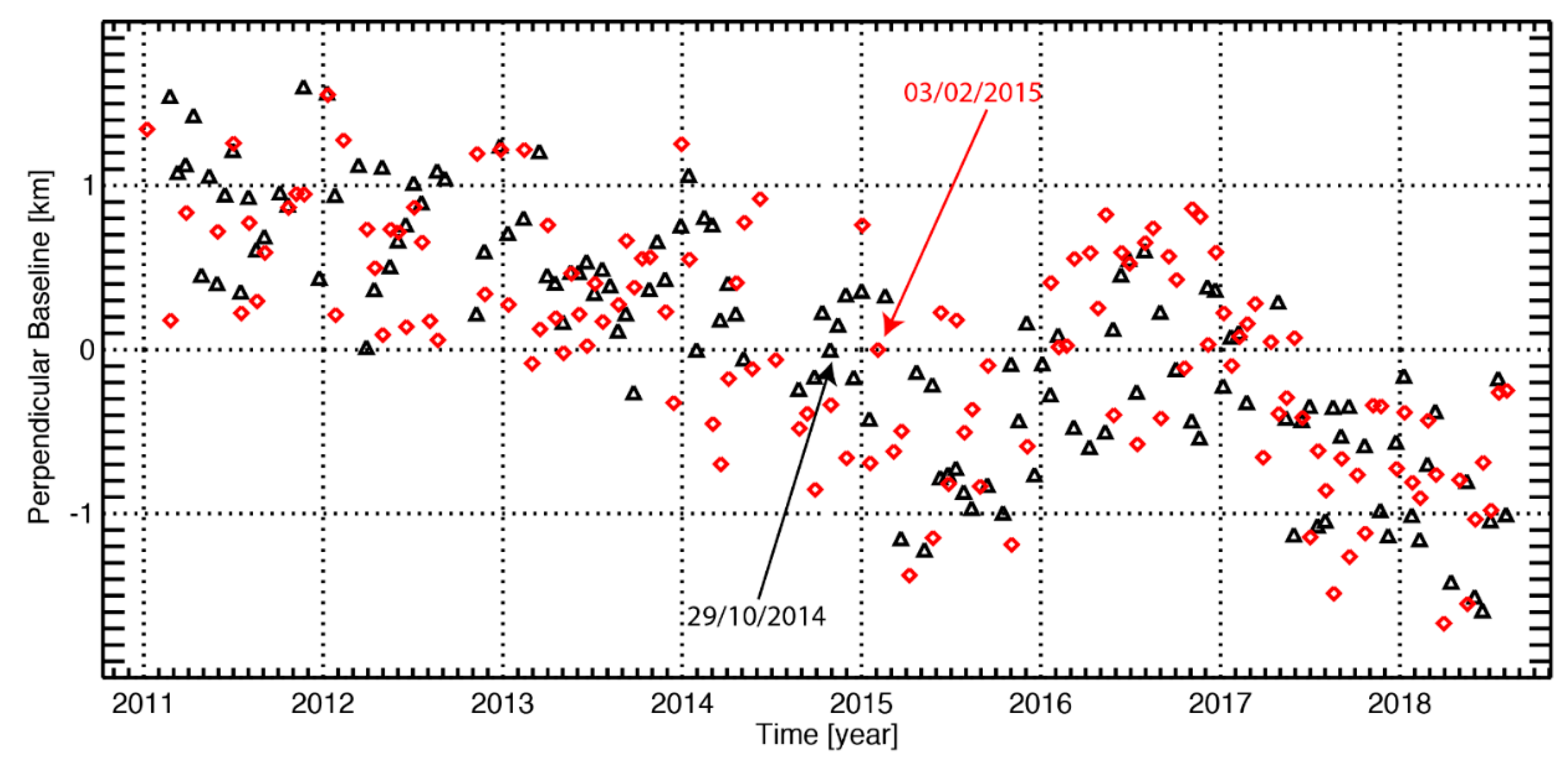
| Time interval | 23 February 2011–5 August 2018 | 7 January 2011–6 August 2018 |
| Number of acquisitions | 132 | 134 |
Publisher’s Note: MDPI stays neutral with regard to jurisdictional claims in published maps and institutional affiliations. |
© 2020 by the authors. Licensee MDPI, Basel, Switzerland. This article is an open access article distributed under the terms and conditions of the Creative Commons Attribution (CC BY) license (http://creativecommons.org/licenses/by/4.0/).
Share and Cite
Lanari, R.; Reale, D.; Bonano, M.; Verde, S.; Muhammad, Y.; Fornaro, G.; Casu, F.; Manunta, M. Comment on “Pre-Collapse Space Geodetic Observations of Critical Infrastructure: The Morandi Bridge, Genoa, Italy” by Milillo et al. (2019). Remote Sens. 2020, 12, 4011. https://0-doi-org.brum.beds.ac.uk/10.3390/rs12244011
Lanari R, Reale D, Bonano M, Verde S, Muhammad Y, Fornaro G, Casu F, Manunta M. Comment on “Pre-Collapse Space Geodetic Observations of Critical Infrastructure: The Morandi Bridge, Genoa, Italy” by Milillo et al. (2019). Remote Sensing. 2020; 12(24):4011. https://0-doi-org.brum.beds.ac.uk/10.3390/rs12244011
Chicago/Turabian StyleLanari, Riccardo, Diego Reale, Manuela Bonano, Simona Verde, Yasir Muhammad, Gianfranco Fornaro, Francesco Casu, and Michele Manunta. 2020. "Comment on “Pre-Collapse Space Geodetic Observations of Critical Infrastructure: The Morandi Bridge, Genoa, Italy” by Milillo et al. (2019)" Remote Sensing 12, no. 24: 4011. https://0-doi-org.brum.beds.ac.uk/10.3390/rs12244011