Bi-Temporal Analysis of Spatial Changes of Boreal Forest Cover and Species in Siberia for the Years 1985 and 2015

Key Lab. of Digital Earth Science, Aerospace Information Research Institute, Chinese Academy of Sciences, Beijing 100094, China
*
Author to whom correspondence should be addressed.
Remote Sens. 2020, 12(24), 4116; https://0-doi-org.brum.beds.ac.uk/10.3390/rs12244116
Submission received: 2 November 2020
/
Revised: 14 December 2020
/
Accepted: 14 December 2020
/
Published: 16 December 2020
(This article belongs to the Special Issue Mapping Tree Species Diversity)
Abstract
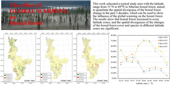
:Boreal forest is a sensitive indicator of the influence of climate change. It can quantify the level and spatial divergence of forest change for forest resources and carbon cycle research. This study selected a typical boreal forest affected by few human activities as a research area, in Siberia, with a latitude span of 51°N–69°N. A total of 150 Landsat images of this area acquired in 1985 and 2015 were collected. A hierarchical classification approach was first established to retrieve the information of forest cover and species. The forested and nonforested lands were discriminated by the decision tree method and, furthermore, the forested land was classified to broad-leaved and coniferous forests by a random forest algorithm. The overall accuracy was 90.37%, which indicates the validity of the approach. Finally, the quantitative information of the forest cover and species changes in each latitude zone of every 2° was analyzed. The results show that the overall boreal forest cover increased by 5.11% over the past three decades, with broad-leaved forest increasing by 3.54% and coniferous forest increasing by 1.57%. In addition, boreal forest increased in every latitude zone, and the spatial divergence of the changes of the boreal forest cover and species in different latitude zones were significant. Finally, broad-leaved forest increased more rapidly than coniferous forest, and the greatest increase, of up to 5.77%, occurred in the zone of 55°N–57°N.
1. Introduction
Forests cover more than one-third of the earth’s land surface. They are one of the critical biomes globally and provide ecosystem services that benefit society at levels ranging from local to global [1,2]. Forests have been shown to strongly interact with climate change [3]. Furthermore, forests can modify the global carbon budget by altering the sequestration and release of carbon to influence climate change. Conversely, climate change has a profound impact on global forestry, and continues to accelerate with increasing anthropogenic greenhouse gas (GHG) emissions [4]. Due to rapid climate change, forest cover and species ranges continue to shift [5]. To a degree, the above coupling process balances climate change, and these influences also cause changes in forest cover and abundance of species. Therefore, quantifying the spatial changes of forest cover and species is important for improving carbon accounting, climate change modeling, and biodiversity monitoring.
It is an indisputable fact that the global climate is now warming [6,7,8,9,10]. Recent years (2015–2018) have been the warmest since 1850 [11,12]. In addition, higher latitudinal areas, such as boreal forest areas, are expected to undergo the largest increases in temperature [13,14,15,16] and experience variable shifts in precipitation regimes [17,18,19]. Global warming has influenced the suitable climate conditions for different forest species, and studies have shown that climate zones in boreal forests are moving northwards ten times faster than trees’ ability to migrate [20,21].
Boreal forests, which span the northern hemisphere across three continents and ten different countries, comprise about 30% of the total forest area globally [20,22] and are considered among the most vulnerable to climate change [13]. The boreal forest is floristically simple and consists of hardy genera of larch (Larix), pine (Pinus), spruce (Picea), and fir (Abies), interspersed with deciduous hardwoods of birch (Betula), aspen (Populus), willow (Salix), and alder (Alnus). With temperatures in the arctic and boreal domains recently warming, boreal forests have been shown as one of the ecosystems most affected by climate change [23]. Furthermore, quantitative rates of the spatial changes of boreal forest cover and species are important indicators for research of the influence of climate change and are helpful for improving carbon accounting and biodiversity monitoring, which are not yet fully understood. A practical solution to examining trends in forest cover change at a large scale is to employ remotely sensed data [24]. Satellite-based monitoring can be implemented consistently across large regions at annual and interannual intervals [25,26,27].
Numerous studies have investigated the effect of climate change on boreal forest by remote sensing techniques. It has been observed that the growth of boreal forest was influenced by global warming over the past decade using Moderate-resolution Imaging Spectroradiometer (MODIS) images; however, there is obvious spatial divergence [28,29]. In practice, it is a challenge to quantify the effects of climate change using remote sensing data with low spatial resolution because, due to the low resolution, it is difficult to distinguish the subtle spatial distribution of different forest species. Furthermore, significant uncertainties are attached to possible interactions among forests and climate change, in addition to other land-use pressures [3].
Landsat images provide an ideal option for remote sensing with a medium spatial resolution of 30 m and temporal resolution of 16 days, thus allowing for monitoring of natural and human-induced landscape changes at local or regional scales over years and decades [30,31]. Landsat satellite data have been most widely adopted for studying vegetation phenology, agriculture and forestry, surface temperature monitoring, and air pollution monitoring due to their high spatial resolution and global coverage [32,33,34,35]. The long-term data record of nearly five decades allows it to be used for forest investigations for any number of time periods. However, longer time series will require more data processing and storage capacity [36].
In this work, we selected a typical study area in Siberia in which the boreal forests have been affected primarily by natural factors to quantify the spatial changes and divergences of boreal forest cover and species over the past three decades using the Landsat series dataset. The aim was to reveal the latitude zones in which the forest cover and species were more sensitive to climate change, and to provide quantitative information for climate change and ecosystem research.
2. Study Area and Datasets
2.1. Study Area
The boreal forest in Krasnoyarskiy Kray in Central Russia, located in the middle of Siberia (Figure 1), was selected as the study area. The approximate latitude range of the area is 51°N to 69°N, and the longitude is 84°E to 110°E. This work concerns the spatial changes of forest cover and forest species related to latitude in the context of climate change. We divided the study area into nine latitude zones by every 2° from south to north. The information for every latitude zone is shown in Table 1. The latitude range of this area is considered sufficiently large for sensitivity analysis of the forest change.
The climate in the area is strongly continental, with large temperature variations from south to north. The territory of the study area experiences the conditions of three climate belts: Arctic, Subarctic, and moderate. For the central and southern regions, long winters and short hot summers are characteristic. In the north, there are fewer than 40 days with temperatures above 10 ℃, whereas, in the south, there are 110–120 such days. The average temperature in January is −36 ℃ in the north and −18 ℃ in the south, and in July it is 10 ℃ in the north and 20 ℃ in the south. The annual precipitation is 200–300 mm in the north and about 1000 mm in the south. Permafrost is widespread in this area, particularly in the north. The south of the permafrost zone is covered by primeval forest, and the forest species are mainly broad-leaved and coniferous. This area is sparsely populated, with a small number of towns and villages spread throughout the south, surrounded by areas of farmland.
2.2. Datasets
A total of 150 Landsat Thematic Mapper (TM) and Operational Land Imager (OLI) series scenes with little to no cloud cover in the study area, collected from the United States Geological Survey (USGS) (http://glovis.usgs.gov/), were used in this work. These images were acquired during 1985 and 2015, respectively. Most of the images were acquired during summer, mainly between June and September. To account for lacking data, three images with no snow over the south area acquired in October were also used. Some data from adjacent years were used to make up the images due to data deficiencies in the current years. The data product is L1T level with a spatial resolution of 30 m.
3. Data Process
3.1. Data Preprocess
The dataset was preprocessed to eliminate radiometric and geometric distortions. Image preprocessing includes radiometric and atmospheric corrections (Figure 2). To minimize the influence of cloud noise, a haze optimized transformation (HOT) algorithm was used to identify and remove thin clouds [37,38,39]. Firstly, the clear line was determined according to the high correlation between the blue and red bands in the clear region, and then the HOT value was calculated using the transform equation:
where ρ1 and ρ3 are the reflectance of the blue and red bands of TM and OLI images, respectively. I represents the intercept of the clear line, and θ is the inclination of the clear line.
The cloud images were classified by the HOT value which represented the cloud thickness, and then the Landsat image in the cloud region and clear region was automatically classified using just one near-infrared band and two shortwave infrared bands. The image in the cloud region of visible bands was matched to the image in the clear region according to the cloud class and object classification to remove the effect of the cloud.
3.2. Forest Classification Approach
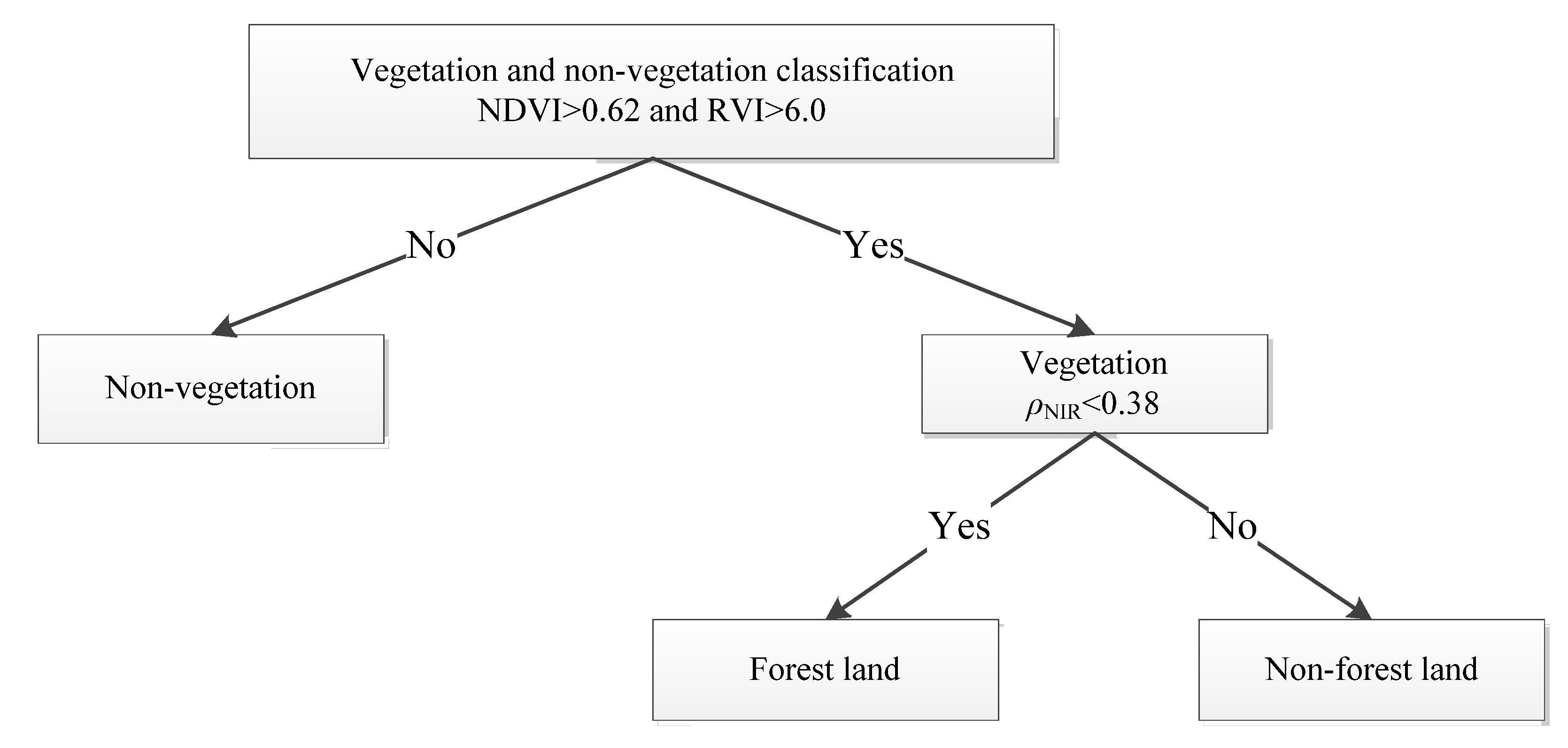
This study focused on the changes of boreal forest coverage and species in Siberia, and a hierarchical information extraction approach was established and used for the forest classification. Firstly, a simple decision tree method was adopted to discriminate between forest and nonforest land in the Landsat images, and then a random forest (RF) algorithm was employed to distinguish the broad-leaved and coniferous species from forest land.
3.2.1. Forest and Nonforest Land Classification by Decision Tree Method
The decision tree algorithm is intuitive and flexible, and has high computational efficiency in processing a large quantity of data. In this classification, two vegetation indices, normalized vegetation index (NDVI) and ratio vegetation index (RVI), were used for the discrimination between forest and nonforest land. NDVI can effectively weaken the effects of complex terrain in image information extraction, and enhance the distinction between vegetation and other land types, which is helpful for improving the accuracy and credibility of forest information extraction. The RVI can better reflect the difference of vegetation growth and coverage, and is suitable for vegetation monitoring in areas with vigorous vegetation growth and high coverage. The annual maximum NDVI (NDVImax) values of built-up areas, barren lands, and sparsely vegetated lands are usually lower than 0.30, whereas forest NDVImax values are usually higher than 0.50 [40]. Subsequently, we determined the decision tree classification rules based on sample training: NDVI values greater than 0.62 and RVI values greater than 6.0 were selected as vegetation land, otherwise land was regarded as nonvegetation land.
Next, we distinguished the vegetation land between forest and other vegetation. We found that different plants have different spectral reflectance peaks in the near-infrared band, which is highly sensitive to the difference in reflectance caused by the internal structure of different leaves. Therefore, the reflectance of the near-infrared band can be used to distinguish forest and other vegetation. The vegetation objects classified in the upper layer with reflectance values in the near-infrared band of less than 0.38 were selected as forest land, otherwise they were categorized as nonforest land. The first layer of nonvegetation land and the second layer of nonforest land were combined as the final nonforest land classification result, and the second layer of forest land classification as the final forested land classification result (Figure 3).
3.2.2. Broad-Leaved and Coniferous Forest Classification by Random Forest Algorithm
The distinction of natural attributes within forest species is limited by the spectral resolution. It is difficult to detect the subtle spectral differences between coniferous forest and broad-leaved forest with a single image spectral feature. Therefore, it is necessary to use a combination of various spectral features and vegetation indices to classify coniferous and broad-leaved forests. To avoid the impact of other ground features, the nonforested lands were masked.
The random forest algorithm is an extension of the concept of the decision tree [41,42,43]. As a common algorithm applied in the field of machine learning, RF is often used as a classification method [44,45,46,47]. Representative training samples are one of the most critical components in the RF algorithm. The quality and distribution of these samples are also important. In this work, we selected the broad-leaved and coniferous forest sample points from Landsat images following the following principles: (1) the training samples must avoid land-cover mixtures and heterogeneous areas; (2) the sample points should be distributed in a scene that is as representative as possible; (3) the forest-cover category must be interpretable using TM images. Additionally, Google Earth images of the same areas were also used as a reference [48]. Six bands, Landsat TM bands 1–5 and 7, and Landsat OLI bands 2–7, were selected as spectral characteristic variables; NDVI, normalized difference index (NDI) [49] and RVI were selected as index characteristic variables for classification in RF. Additionally, in the RF algorithm, the parameter ntree controls the growth number of decision trees, and another parameter mtry represents the maximum number of features randomly selected from the above nine variables in the individual tree. In this study, considering the computational efficiency and classification accuracy, the values of ntree and mtry were set to 1000 and 3, respectively. Finally, the broad-leaved and coniferous forests were classified using the above random sample points using the RF algorithm.
3.2.3. Accuracy Assessment
In this study, four simultaneous Gaofen-2 (GF-2) satellite panchromatic band images acquired in 2015 were used to validate the classification results. The spatial resolution of GF-2 images was 0.81 m. We selected 987 randomly distributed sampling points from GF-2 images for the validation, and the overall accuracy (OA) and F1-score were calculated to evaluate the reliability of the classification results [50], as shown in Table 2. The overall accuracy was 90.37%, and the F1-scores of broad-leaved, coniferous and nonforest land were 0.85, 0.93, and 0.91, respectively. Considering the consistency of the Landsat series images, the above validation result is still considered to be valid for 1985 because it is difficult to obtain the measured data or the high-resolution satellite images of the study area for 1985.
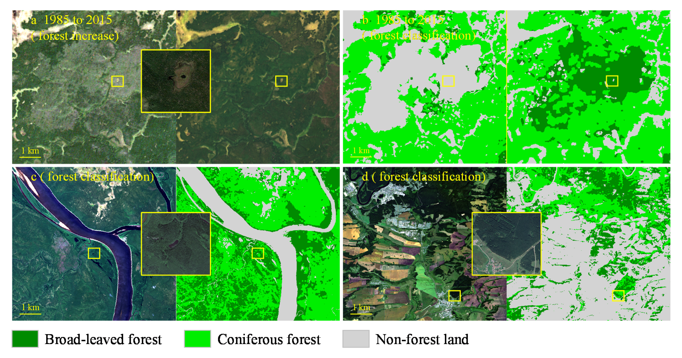
Moreover, the tree-cover-2010 data from Global Forest Watch (GFW) was also used to validate the classification results by spatial overlay analysis [51]. The GFW project is focused on developing global tree cover change data products based on Landsat satellite imagery, and provides global tree cover data with a resolution of 30 m [52]. The spatial consistency of the tree-cover-2010 data and our classification results of forest land was 85.26%. Additionally, Figure 4 presents examples of classified scenes from various areas.
4. Result and Analysis
4.1. Spatial Change of Boreal Forest Cover
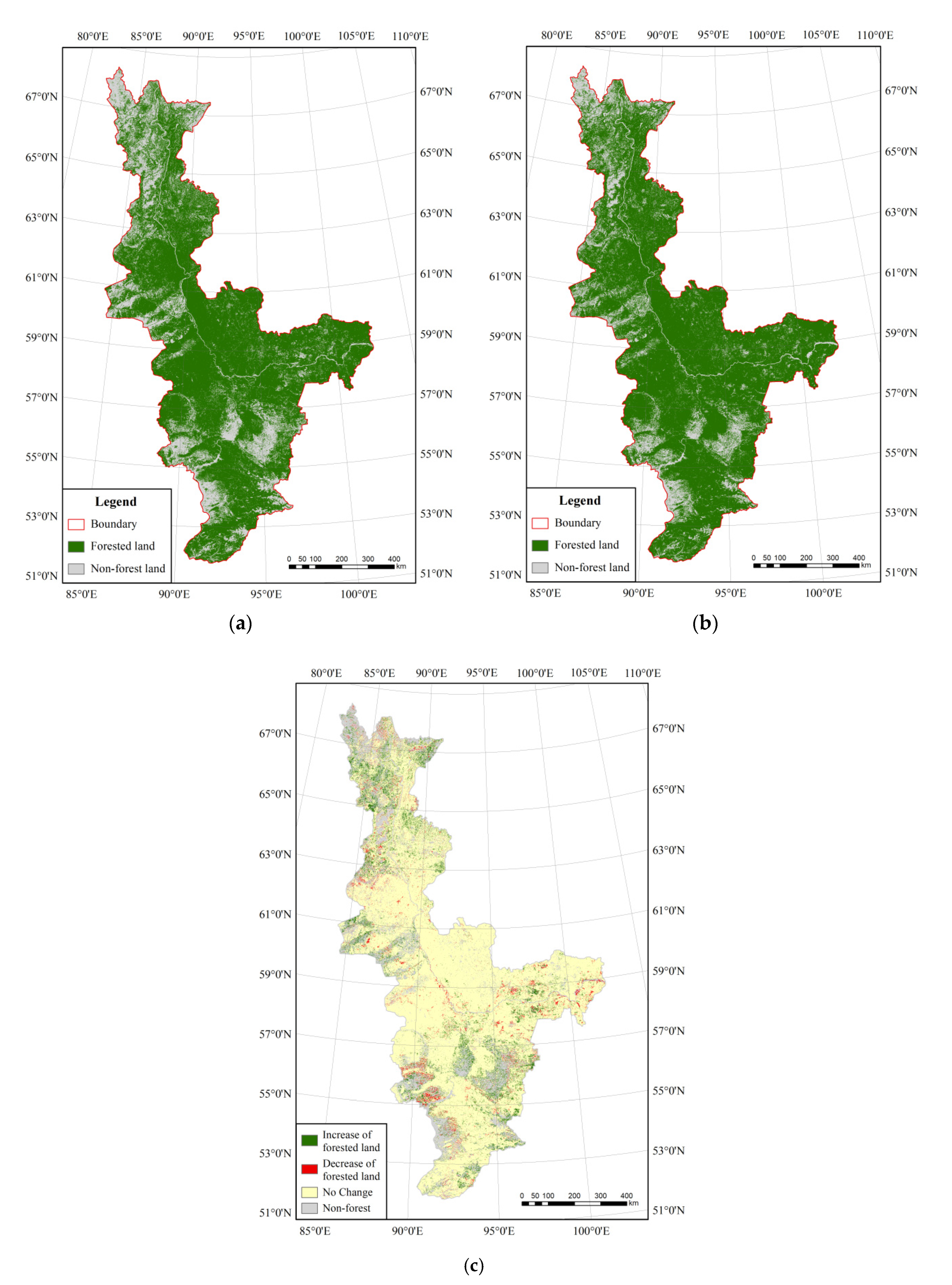
Firstly, the forest and nonforest lands in the two periods of 1985 and 2015 were classified, and the results are shown in Figure 5a,b. The spatial change of the boreal forest cover between the two years is shown in Figure 5c, and the quantitative information is displayed in Table 3 and Figure 6.
From Figure 5 and Table 3, it can be seen that substantial change has occurred in the boreal forest cover in the research area over the past three decades. Overall, the rate of forest cover Rfl, expressed as the ratio between the area of forest land and the total land area, increased by 5.11% from 75.42% to 80.52%, and Rfl was high in the south and low in the north. In 53°N–57°N, human activities occurred that slightly reduced the forest cover. In the region 57°N–69°N, the forest cover and change were mainly influenced by natural factors, with little human activity taking place. The largest rate of forest cover was in 57°N–59°N, of about 91.00%, in 2015. In the latitude zone 67°N–69°N, the north border of the boreal forest, Rfl was as high as 34.35% in 2015.
In this research, we were particularly concerned about the quantitative spatial divergence of the forest change in different latitude zones. Thus, we calculated the change of forest cover rate ΔRfl between 1985 and 2015 for every latitude zone to reflect the absolute change velocity of forest cover (Table 3). It can be seen that the rates of forest cover increased in all latitude zones from 1985 to 2015, although with a clear divergence. Compared to other zones, the increase in forest cover was greatest in the north region from 63°N to 69°N, and the greatest increase was up to 13.50% in 65°N–67°N, indicating that the forest cover was more sensitive to climate change in this latitude zone. A relatively slow increase of 1.00% occurred in the latitude zone from 57°N to 59°N, in which the forest cover was up to about 91.00% (Figure 6).
Additionally, we also calculated ΔRfo, expressed as the ratio between the area of changed forest cover and the original forest land, which can be used to reflect the relative increase rate of the forest area itself. The result shows that the greatest ΔRfo was up to 24.61% in the latitude zone 65°N–67°N (Figure 6), which indicates that the forest has the strongest regeneration ability in this region against the background of global warming.
4.2. Spatial Changes of Boreal Forest Species
The broad-leaved and coniferous forests were distinguished from forest land, as shown in Figure 7a,b, and the quantitative information of the two forest species is shown Table 4. The total broad-leaved forest area in the research region increased by 39,341.30 km2 over the past three decades. Overall, the broad-leaved and coniferous forest cover increased in the research area. First, we calculated the ratio Rbl between the areas of broad-leaved forest and the total land, and Rcl for the coniferous forest. These two ratios can be used to reflect the absolute cover of the two forest species of the total land. The line charts of the cover and change of the forest species are shown in Figure 8. In the study area, the broad-leaved forest cover increased by 3.54%, from 23.83% to 27.37%, and coniferous forest increased by 1.57%, from 51.58% to 53.15%. It also can be seen that overall coniferous forest was more dominant than broad-leaved forest during the study period; however, the broad-leaved forest increased more rapidly than the coniferous forest.
We also analyzed the spatial divergence of the cover of each forest species in different latitude zones. The largest Rbl was about 45.00%, and occurred in the latitude zone 55°N–57°N in 2015. It can also be seen that, in 51°N–65°N, the change trend of Rbl and Rcl were almost contrary with the latitude zones (Figure 8a). Rbl and Rcl were both lowest in the 67°N–69°N zone, which was the north border of boreal forest in Siberia, with values of about 5.35% and 29.00% in 2015, respectively.
The ratio Rbo between the area of broad-leaved forest and the area of forested land, and Rco for coniferous forest, can be used to reflect the abundances of the two forest species in the forested land. The broad-leaved forest was the dominant species in 53°N–57°N (Figure 8b). However, in the 51°N–53°N zone, the Rbo of broad-leaved forest was about 32.79% in 1985 and 35.59% in 2015, and significantly less than that in 53°N–57°N. This is because the average altitude is over 1000 m in the 51°N–53°N zone, which is significantly higher than that of about 450 m in 53°N–57°N. In the latitude zones from 57°N to 69°N, coniferous forests were more abundant than broad-leaved forests, mainly due to the relatively cold weather in this region. However, an abnormal phenomenon is that Rbl in the 59°N–61°N zone was almost the lowest in the research area, and surprisingly was substantially lower than that in 63°N–65°N, which may be due to the influence of multiple factors, such as climate and artificial logging.
It is important for carbon cycle research that the spatial divergence of the boreal forest species changes in different latitude zones (Figure 8c,d). Here, we firstly calculated ΔRbl and ΔRbo, which represent the changes of Rbl and Rbo over the past three decades, respectively (Table 4 and Figure 8c). It can be seen that the broad-leaved forest cover Rbl increased in all latitude zones. The greatest increase was up to 5.77% in 55°N–57°N. The lowest was about 0.45% in 67°N–69°N, which can be considered to represent no change in the broad-leaved forest cover in this zone considering the accuracy of the classification. We also note that the change of Rbl was about 1.33% in 59°N–61°N, which is relatively low compared with other latitude zones, with the exception of 67°N–69°N. The explanation for this phenomenon requires further study. ΔRbo in 67°N–69°N was −0.89%, which indicates that the proportion of broad-leaved forest decreased slightly in this zone, although Rbl increased.
In addition, ΔRcl was also calculated, and represents the change of Rcl over the past three decades (Figure 8d). It can be seen that the coniferous forest cover decreased in the zones 57°N–59°N and 61°N–63°N; however, coniferous forest increased significantly in the latitude from 65°N to 69°N, where broad-leaved forest increased relatively slowly.
5. Conclusions
Boreal forests have been affected by climate change over the past three decades, which is predominantly reflected in the changes of forest cover and species. This work selected a typical area in central Siberia, and collected 150 Landsat TM/OLI images covering this area acquired in 1985 and 2015. A hierarchical classification process was established for the retrieval of boreal forest cover and species. Finally, quantitative spatial information of the forest cover and species was compiled for latitude zones for every 2°. The results show that the impact of climate change on the boreal forest has a significant spatial divergence. Compared with other zones, the increase in forest cover was greatest in the region from 63°N to 69°N, indicating that the forest cover was more sensitive to climate change in this region. Furthermore, the broad-leaved forest cover increased by 3.54% and coniferous forest increased by 1.57%. Overall, coniferous forest was also more dominant than broad-leaved forest during the study period, although broad-leaved forest increased more rapidly than coniferous forest. In 67°N–69°N, the proportion of broad-leaved forest decreased slightly.
This study considered only two periods, i.e., 1985 and 2015. However, it will be necessary in future work to study forest change during other periods. In addition, more research is required to determine which climate factors, such as temperature or precipitation, are the main driving forces of forest change.
Author Contributions
Conceptualization, W.F.; methodology, W.F. and L.T.; investigation, L.T. Both wrote the original draft and performed the final review. All authors have read and agreed to the published version of the manuscript.
Funding
This work was supported by the Strategic Priority Research Program of the Chinese Academy of Sciences (XDA19070102) and supported by the National Natural Science Foundation of China (No. 61971417).
Conflicts of Interest
The authors declare no conflict of interest.
References
- Trumbore, S.; Brando, P.; Hartmann, H. Forest health and global change. Science 2015, 349, 814–818. [Google Scholar] [CrossRef] [PubMed] [Green Version]
- Bos, A.B.; Sy, V.D.; Duchelle, A.E.; Herold, M.; Martius, C.; Tsendbazar, N.E. Global data and tools for local forest cover loss and REDD+ performance assessment: Accuracy, uncertainty, complementarity and impact. Int. J. Appl. Earth Obs. Geoinf. 2019, 80, 295–311. [Google Scholar] [CrossRef]
- Price, D.T.; Alfaro, R.I.; Brown, K.J.; Flannigan, M.D.; Fleming, R.A.; Hogg, E.H. Anticipating the consequences of climate change for Canada’s boreal forest ecosystems1. Environ. Rev. 2013, 21, 322–365. [Google Scholar] [CrossRef]
- IPCC. Summary for policy makers. In Climate Change 2014: Synthesis Report. Contibution of Working Groups I, II, and III to the Fifth Assessment Report if the Intergovernmental Panel on Climate Change; IPCC: Geneva, Switzerland, 2014. [Google Scholar]
- Pecl, G.T.; Araújo, M.B.; Bell, J.D.; Blanchard, J.; Bonebrake, T.C.; Chen, I.C. Biodiversity redistribution under climate change: Impacts on ecosystems and human well-being. Science 2017, 355, 1–9. [Google Scholar] [CrossRef] [PubMed]
- Folland, C.K.; Karl, T.R.; Christy, J.R.; Clarke, R.A.; Gruza, G.V.; Jouzel, J.; Mann, M.E.; Oerlemands, J.; Salinger, M.J.; Wang, S.W. Observed climate variability and change. In The Scientific Basis: Contribution of Working Group I to the Third Assessment Report of the Intergovernmental Panel on Climate Change; Cambridge University Press: New York, NY, USA, 2001; pp. 99–181. [Google Scholar]
- Thuiller, W. Biodiversity: Climate change and the ecologist. Nature 2007, 448, 550–552. [Google Scholar] [CrossRef] [PubMed]
- Gauthier, S.; Bernier, P.; Burton, P.J.; Edwards, J.; Isaac, K.; Isabel, N.; Jayen, K.; Le Goff, H.; Nelson, E.A. Climate change vulnerability and adaptation in the managed. Environ. Rev. 2014, 22, 256–285. [Google Scholar] [CrossRef]
- Lawal, S.; Lennard, C.; Hewitson, B. Response of southern African vegetation to climate change at 1.5 and 2.0° global warming above the pre-industrial level. Clim. Serv. 2019, 16, 1–16. [Google Scholar] [CrossRef]
- Engelbrecht, C.J.; Engelbrecht, F.A. Shifts in Köppen-Geiger climate zones over southern Africa in relation to key global temperature goals. Theor. Appl. Climatol. 2015, 123, 247–261. [Google Scholar] [CrossRef]
- Jones, P.D.; Osborn, T.J. Climate record: Surface temperature trends. In Reference Module in Earth Systems and Environmental Sciences; 2018; pp. 110–120. Available online: https://0-doi-org.brum.beds.ac.uk/10.1016/B978-0-12-382225-3.00005-0 (accessed on 16 December 2020).
- Kumar, A.; Yadav, J.; Mohan, R. Global warming leading to alarming recession of the Arctic sea-ice cover: Insights from remote sensing observations and model reanalysis. Heliyon 2020, 6, 1–10. [Google Scholar] [CrossRef]
- Diffenbaugh, N.S.; Field, C.B. Changes in ecologically critical terrestrial climate conditions. Science 2013, 341, 486–492. [Google Scholar] [CrossRef] [Green Version]
- Ouyang, W.; Gao, X.; Hao, Z.; Liu, H.; Hao, F. Farmland shift due to climate warming and impacts on temporal-spatial distributions of water resources in a middle-high latitude agricultural watershed. J. Hydrol. 2017, 547, 156–167. [Google Scholar] [CrossRef]
- Sun, Q.; Miao, C.; Duan, Q. Projected changes in temperature and precipitation in ten river basins over China in 21st century. Int. J. Climatol. 2015, 35, 1125–1141. [Google Scholar] [CrossRef]
- Huang, J.; Zhang, X.; Zhang, Q.; Lin, Y.; Hao, M.; Luo, Y.; Zhao, Z.; Yao, Y.; Chen, X.; Wang, L.; et al. Recently amplified arctic warming has contributed to a continual global warming trend. Nat. Clim. Chang. 2017, 7, 875–879. [Google Scholar] [CrossRef]
- Gauthier, S.; Bernier, P.; Kuuluvainen, T.; Shvidenko, A.Z.; Schepaschenko, D.G. Boreal forest health and global change. Science 2015, 349, 819–822. [Google Scholar] [CrossRef]
- Reyer, C.P.O.; Brouwers, N.; Rammig, A.; Brook, B.W.; Epila, J.; Grant, R.F. Forest resilience and tipping points at different spatio-temporal scales: Approaches and challenges. J. Ecol. 2015, 103, 5–15. [Google Scholar] [CrossRef] [Green Version]
- Donnelly, C.; Wouter, G.; Andersson, J.; Gerten, D.; Pisacane, G.; Roudier, P.; Ludwig, F. Impacts of climate change on European hydrology at 1.5, 2 and 3 degree mean global warming above preindustrial level. Clim. Chang. 2017, 143, 13–26. [Google Scholar] [CrossRef] [Green Version]
- Soja, A.J.; Tchebakova, N.M.; French, N.H.F.; Flannigan, M.D.; Shugart, H.H.; Stocks, B.J.; Sukhinin, A.I.; Parfenova, E.I.; Chapin, F.S.; Stackhouse, P.W. Climate-induced boreal forest change: Predictions versus current observations. Glob. Planet. Chang. 2007, 56, 274–296. [Google Scholar] [CrossRef] [Green Version]
- Toshichika, I.; Ramankutty, N. How do weather and climate influence cropping area and intensity? Glob. Food Secur. 2015, 4, 46–50. [Google Scholar]
- Brecka, A.F.J.; Shahi, C.; Chen, H.Y.H. Climate change impacts on boreal forest timber supply. For. Policy Econ. 2018, 92, 11–21. [Google Scholar] [CrossRef]
- Oboite, F.O.; Comeau, P.G. Competition and climate influence growth of black spruce in western boreal forests. For. Ecol. Manag. 2019, 443, 84–94. [Google Scholar] [CrossRef]
- Kivinen, S.; Koivisto, E.; Keski-Saari, S.; Poikolainen, L.; Tanhuanpää, T.; Kuzmin, A.; Viinikka, A.; Heikkinen, R.K.; Pykälä, J.; Virkkala, R.; et al. A keystone species, European aspen (Populus tremula L.), in boreal forests: Ecological role, knowledge needs and mapping using remote sensing. For. Ecol. Manag. 2020, 462, 118008. [Google Scholar] [CrossRef]
- Ols, C.; Kålås, I.H.; Drobyshev, I.; Söderström, L.; Hofgaard, A. Spatiotemporal variation in the relationship between boreal forest productivity proxies and climate data. Dendrochronologia 2019, 58, 125648. [Google Scholar] [CrossRef]
- Kato, A.; Thau, D.; Hudak, A.T.; Meigs, G.W.; Moskal, L.M. Quantifying fire trends in boreal forests with Landsat time series and self-organized criticality. Remote Sens. Environ. 2020, 237, 111525. [Google Scholar] [CrossRef]
- Moreno-Martínez, Á.; Camps-Valls, G.; Kattge, J.; Robinsona, N.; Reichstein, M.; van Bodegom, P.; Kramer, K.; Cornelissen, J.H.C.; Reich, P.; Bahn, M.; et al. A methodology to derive global maps of leaf traits using remote sensing and climate data. Remote Sens. Environ. 2018, 218, 69–88. [Google Scholar] [CrossRef] [Green Version]
- Hou, M.; Venäläinen, A.K.; Wang, L.; Pirinen, I.P.; Gao, Y.; Jin, S.; Zhu, Y.; Qin, F.; Hu, Y. Spatio-temporal divergence in the responses of Finland’s boreal forests to climate variables. Int. J. Appl. Earth Obs. Geoinf. 2020, 92, 1–9. [Google Scholar] [CrossRef]
- Alibakhshi, S.; Naimi, B.; Hovi, A.; Crowther, T.W.; Rautiainen, M. Quantitative analysis of the links between forest structure and land surface albedo on a global scale. Remote Sens. Environ. 2020, 246, 1–12. [Google Scholar] [CrossRef]
- Rendenieks, Z.; Nita, M.D.; Nikodemus, O.; Radeloff, V.C. Half a century of forest cover change along the Latvian-Russian border captured by object-based image analysis of Corona and Landsat TM/OLI data. Remote Sens. Environ. 2020, 249, 1–14. [Google Scholar] [CrossRef]
- Senf, C.; Laštovička, J.; Okujeni, A.; Heurich, M.; Linden, S. A generalized regression-based unmixing model for mapping forest cover fractions throughout three decades of Landsat data. Remote Sens. Environ. 2020, 240, 1–10. [Google Scholar] [CrossRef]
- Wulder, M.; Loveland, T.; Roy, D.; Crawford, C.; Masek, J.; Woodcock, C. Current status of Landsat program, science, and applications. Remote Sens. Environ. 2019, 225, 127–147. [Google Scholar] [CrossRef]
- Wu, Z.; Snyder, G.; Vadnais, C.; Arora, R.; Babcock, M.; Stensaas, G.; Doucette, P.; Newman, T. User needs for future Landsat missions. Remote Sens. Environ. 2019, 231, 1–13. [Google Scholar] [CrossRef]
- Jönsson, P.; Cai, Z.; Melaas, E.; Friedl, M.A.; Eklundh, L. A method for robust estimation of vegetation seasonality from Landsat and sentinel-2 time series data. Remote Sens. 2018, 10, 635. [Google Scholar] [CrossRef] [Green Version]
- Restrepo, A.M.C.; Yang, Y.R.; Hamm, N.A.; Gray, D.J.; Barnes, T.S.; Williams, G.M.; Clements, A.C. Land cover change during a period of extensive landscape restoration in Ningxia Hui autonomous region. China Sci. Total Environ. 2017, 598, 669–679. [Google Scholar] [CrossRef]
- Bolton, D.K.; Tompalski, P.; Coops, N.C.; White, J.C.; Wulder, M.A.; Hermosilla, T.; Queinnec, M.; Luther, J.E.; Lier, O.R.; Fournier, R.A.; et al. Optimizing Landsat time series length for regional mapping of lidar-derived forest structure. Remote Sens. Environ. 2020, 239, 111645. [Google Scholar] [CrossRef]
- Zhang, Y.; Guindon, B.; Cihlar, J. An image transform to characterize and compensate for spatial variations in thin cloud contamination of Landsat images. Remote Sens. Environ. 2002, 82, 173–187. [Google Scholar] [CrossRef]
- Li, W.; Li, Y.; Chen, D.; Chan, J.C. Thin cloud removal with residual symmetrical concatenation network. ISPRS J. Photogramm. Remote Sens. 2019, 153, 137–150. [Google Scholar] [CrossRef]
- Liu, Q.; Gao, X.; He, L.; Lu, W. Haze removal for a single visible remote sensing image. Signal Process. 2017, 137, 33–43. [Google Scholar] [CrossRef]
- Qin, Y.; Xiao, X.; Dong, J.; Zhang, G.; Shimada, M.; Liu, J. Forest cover maps of china in 2010 from multiple approaches and data sources: PALSAR, Landsat, MODIS, FRA, and NFI. ISPRS J. Photogramm. Remote Sens. 2015, 109, 1–16. [Google Scholar] [CrossRef] [Green Version]
- Breiman, L. Random forests. Mach. Learn. 2001, 45, 5–32. [Google Scholar] [CrossRef] [Green Version]
- Strobl, C.; Boulesteix, A.L.; Zeileis, A.; Hothorn, T. Bias in random forest variable importance measures: Illustrations, sources and a solution. BMC Bioinform. 2007, 8, 25. [Google Scholar] [CrossRef] [Green Version]
- Cutler, D.R.; Edwards, J.T.C.; Beard, K.H.; Cutler, A.; Hess, K.T.; Gibson, J.; Lawler, J.J. Random forest for classification in ecology. ESA Online J. 2008. [Google Scholar] [CrossRef]
- Svetnik, V.; Liaw, A.; Tong, C.; Culberson, J.C.; Sheridan, R.P.; Feuston, B.P. Random forest: A classification and regression tool for compound classification and QSAR modeling. J. Chem. Inf. Comput. Sci. 2003, 43, 1947–1958. [Google Scholar] [CrossRef]
- Rodriguez-Galiano, V.F.; Ghimire, B.; Rogan, J.; Chica-Olmo, M.; Rigol-Sanchez, J.P. An assessment of the effectiveness of a random forest classifier for land-cover classification. ISPRS J. Photogramm. Remote Sens. 2012, 67, 93–104. [Google Scholar] [CrossRef]
- Assiri, A. Anomaly classification using genetic algorithm-based random forest model for network attack detection. Comput. Mater. Contin. 2021, 66, 769–778. [Google Scholar] [CrossRef]
- Climent, F.; Momparler, A.; Carmona, P. Anticipating bank distress in the Eurozone: An Extreme Gradient Boosting approach. J. Bus. Res. 2019, 101, 885–896. [Google Scholar] [CrossRef]
- Gong, P.; Wang, J.; Yu, L.; Zhao, Y.C.; Zhao, Y.Y.; Liang, L.; Niu, Z.G.; Huang, X.M.; Fu, H.H.; Liu, S.; et al. Fine resolution observation and monitoring of global land cover: First mapping results with Landsat TM and ETM+ data. Int. J. Remote Sens. 2013, 34, 2607–2654. [Google Scholar] [CrossRef] [Green Version]
- Rodríguez-Moreno, V.M.; Bullock, S.H. Vegetation response to hydrologic and geomorphic factors in an arid region of the Baja California Peninsula. Environ. Monit. Assess. 2014, 186, 1009–1021. [Google Scholar] [CrossRef] [Green Version]
- Pontius, R.G., Jr.; Millones, M. Death to Kappa: Birth of quantity disagreement and allocation disagreement for accuracy assessment. Int. J. Remote Sens. 2011, 32, 4407–4429. [Google Scholar] [CrossRef]
- Zhao, K.; Jin, B.; Fan, H.; Song, W.; Zhou, S.; Jiang, Y. High-performance overlay analysis of massive geographic polygons that considers shape complexity in a cloud environment. ISPRS Int. J. Geo-Inf. 2019, 8, 290. [Google Scholar] [CrossRef] [Green Version]
- Hansen, M.C.; Potapov, P.V.; Moore, R.; Hancher, M.; Turubanova, S.A.; Thau, D.; Stehman, S.V.; Goetz, S.J.; Loveland, T.R.; Kommareddy, A.; et al. High-resolution global maps of 21st-century forest cover change. Science 2013, 342, 850–853. [Google Scholar] [CrossRef] [Green Version]
Figure 1.
Location of the study area.

Figure 2.
Preprocessing of Landsat Thematic Mapper (TM)/Operational Land Imager (OLI) scenes.

Figure 3.
TM/OLI scene classification based on the decision tree classification model.

Figure 4.
Typical classified scenes in various areas. (a) Images of forest increase; (b) classification results of the images in (a); (c,d) forest classification results in different areas.
Figure 4.
Typical classified scenes in various areas. (a) Images of forest increase; (b) classification results of the images in (a); (c,d) forest classification results in different areas.

Figure 5.
Forest and nonforest land classification: (a) in 1985; (b) in 2015; (c) the spatial change of the forest and nonforest lands.
Figure 5.
Forest and nonforest land classification: (a) in 1985; (b) in 2015; (c) the spatial change of the forest and nonforest lands.

Figure 6.
Line chart of the rates and the changes of forest cover in different latitude zones.

Figure 7.
Broad-leaf forest and coniferous forest classification: (a) 1985; (b) 2015; (c) change in the broad-leaved forest; (d) change in the coniferous forest.
Figure 7.
Broad-leaf forest and coniferous forest classification: (a) 1985; (b) 2015; (c) change in the broad-leaved forest; (d) change in the coniferous forest.


Figure 8.
Spatial divergence of the cover and change of forest species with different latitude zones: (a) Rbl and Rcl in 1985 and 2015; (b) Rbo in 1985 and 2015; (c) ΔRbl and ΔRbo; (d) ΔRcl.
Figure 8.
Spatial divergence of the cover and change of forest species with different latitude zones: (a) Rbl and Rcl in 1985 and 2015; (b) Rbo in 1985 and 2015; (c) ΔRbl and ΔRbo; (d) ΔRcl.


Table 1.
The areas of each latitude zone.
| Latitude Zones (°N) | Area (km2) |
| 67–69 | 19,596.45 |
| 65–67 | 58,813.18 |
| 63–65 | 58,364.09 |
| 61–63 | 66,364.15 |
| 59–61 | 130,507.24 |
| 57–59 | 155,232.73 |
| 55–57 | 114,456.67 |
| 53–55 | 77,579.58 |
| 51–53 | 33,564.27 |
| Total | 714,478.36 |
Table 2.
Accuracy assessment using Gaofen-2 (GF-2) images.
| Land Classification | GF-2 Results | ||||
|---|---|---|---|---|---|
| Broad-Leaved Forest | Coniferous Forest | Nonforest Land | Total | ||
| Landsat Results | Broad-leaved forest | 202 | 12 | 22 | 236 |
| Coniferous forest | 29 | 421 | 24 | 474 | |
| Nonforest land | 8 | 0 | 269 | 277 | |
| Total | 239 | 433 | 315 | 987 | |
| F1-score | 0.85 | 0.93 | 0.91 | ||
| Overall accuracy = 90.37% | |||||
Table 3.
Forest land area and ratio.
| Latitude Zone (°N) | 1985 | 2015 | 1985–2015 | |
|---|---|---|---|---|
| Rfl | Rfl | ΔRfl | ΔRfo | |
| 67–69 | 29.80% | 34.35% | 4.55% | 15.28% |
| 65–67 | 54.84% | 68.34% | 13.50% | 24.61% |
| 63–65 | 68.68% | 77.52% | 8.84% | 12.87% |
| 61–63 | 84.25% | 85.82% | 1.57% | 1.86% |
| 59–61 | 81.73% | 84.97% | 3.24% | 3.96% |
| 57–59 | 89.99% | 90.99% | 1.00% | 1.11% |
| 55–57 | 69.07% | 77.03% | 7.96% | 11.52% |
| 53–55 | 68.65% | 74.93% | 6.28% | 9.14% |
| 51–53 | 77.64% | 82.66% | 5.02% | 6.47% |
| Total | 75.42% | 80.52% | 5.11% | 6.77% |
Table 4.
Broad-leaved forest area.
| Latitude Zone (°N) | Broad-Leaved Forest | Coniferous Forest | |||||||||
|---|---|---|---|---|---|---|---|---|---|---|---|
| 1985 | 2015 | 1985–2015 | 1985 | 2015 | 1985–2015 | ||||||
| Rbl | Rbo | Rbl | Rbo | ΔRbl | ΔRbo | Rcl | Rco | Rcl | Rco | ΔRcl | |
| 67–69 | 4.91% | 16.47% | 5.35% | 15.59% | 0.45% | −0.89% | 24.89% | 83.53% | 29.00% | 84.41% | 4.11% |
| 65–67 | 14.08% | 25.68% | 17.97% | 26.29% | 3.89% | 0.62% | 40.76% | 74.32% | 50.37% | 73.71% | 9.61% |
| 63–65 | 17.51% | 25.50% | 21.41% | 27.61% | 3.89% | 2.11% | 51.17% | 74.50% | 56.11% | 72.39% | 4.95% |
| 61–63 | 14.47% | 17.18% | 18.22% | 21.23% | 3.74% | 4.05% | 69.77% | 82.82% | 67.60% | 78.77% | −2.18% |
| 59–61 | 12.03% | 14.71% | 13.36% | 15.72% | 1.33% | 1.01% | 69.71% | 85.29% | 71.62% | 84.28% | 1.91% |
| 57–59 | 28.20% | 31.34% | 31.92% | 35.08% | 3.72% | 3.74% | 61.79% | 68.66% | 59.07% | 64.92% | −2.72% |
| 55–57 | 39.22% | 56.78% | 44.99% | 58.41% | 5.77% | 1.63% | 29.85% | 43.22% | 32.04% | 41.59% | 2.19% |
| 53–55 | 36.50% | 53.17% | 39.98% | 53.35% | 3.47% | 0.18% | 32.15% | 46.83% | 34.96% | 46.65% | 2.80% |
| 51–53 | 25.46% | 32.79% | 29.42% | 35.59% | 3.96% | 2.79% | 52.18% | 67.21% | 53.25% | 64.41% | 1.06% |
| Total | 23.83% | 31.60% | 27.37% | 33.99% | 3.54% | 2.39% | 51.58% | 68.40% | 53.15% | 66.01% | 1.57% |
Publisher’s Note: MDPI stays neutral with regard to jurisdictional claims in published maps and institutional affiliations. |
© 2020 by the authors. Licensee MDPI, Basel, Switzerland. This article is an open access article distributed under the terms and conditions of the Creative Commons Attribution (CC BY) license (http://creativecommons.org/licenses/by/4.0/).
Share and Cite
MDPI and ACS Style
Tian, L.; Fu, W. Bi-Temporal Analysis of Spatial Changes of Boreal Forest Cover and Species in Siberia for the Years 1985 and 2015. Remote Sens. 2020, 12, 4116. https://0-doi-org.brum.beds.ac.uk/10.3390/rs12244116
AMA Style
Tian L, Fu W. Bi-Temporal Analysis of Spatial Changes of Boreal Forest Cover and Species in Siberia for the Years 1985 and 2015. Remote Sensing. 2020; 12(24):4116. https://0-doi-org.brum.beds.ac.uk/10.3390/rs12244116
Chicago/Turabian StyleTian, Lei, and Wenxue Fu. 2020. "Bi-Temporal Analysis of Spatial Changes of Boreal Forest Cover and Species in Siberia for the Years 1985 and 2015" Remote Sensing 12, no. 24: 4116. https://0-doi-org.brum.beds.ac.uk/10.3390/rs12244116
Note that from the first issue of 2016, this journal uses article numbers instead of page numbers. See further details here.