Hyperspectral Nonlinear Unmixing by Using Plug-and-Play Prior for Abundance Maps

Abstract

Spectral unmixing (SU) aims at decomposing the mixed pixel into basic components, called endmembers with corresponding abundance fractions. Linear mixing model (LMM) and nonlinear mixing models (NLMMs) are two main classes to solve the SU. This paper proposes a new nonlinear unmixing method base on general bilinear model, which is one of the NLMMs. Since retrieving the endmembers’ abundances represents an ill-posed inverse problem, prior knowledge of abundances has been investigated by conceiving regularizations techniques (e.g., sparsity, total variation, group sparsity, and low rankness), so to enhance the ability to restrict the solution space and thus to achieve reliable estimates. All the regularizations mentioned above can be interpreted as denoising of abundance maps. In this paper, instead of investing effort in designing more powerful regularizations of abundances, we use plug-and-play prior technique, that is to use directly a state-of-the-art denoiser, which is conceived to exploit the spatial correlation of abundance maps and nonlinear interaction maps. The numerical results in simulated data and real hyperspectral dataset show that the proposed method can improve the estimation of abundances dramatically compared with state-of-the-art nonlinear unmixing methods.

1. Introduction

Hyperspectral remote sensing imaging is a combination of imaging technology and spectral technology. It can obtain two-dimensional spatial information and spectral information of target objects simultaneously [1,2,3]. Benefiting from the rich spectral information, hyperspectral images (HSIs) can be used to identity materials precisely. Hence, HSIs have been playing a key role in earth observation and used in many fields, including mineral exploration, water pollution, and vegetation [3,4,5,6,7,8,9]. However, due to the low spatial resolution, mixed pixels always exist in HSIs, and it is one of the main reasons that preclude the widespread use of HSIs in precise target detection and classification applications. So it is necessary to develop the technique of unmixing [2,3,10,11,12,13,14]. Thanks to the rich band information of hyperspectral images, which allows us to design an effective solution to the problem of mixed pixels. Hyperspectral unmixing (HU) is the process of obtaining the basic components (called endmembers) and their corresponding component ratios (called abundance fractions). The spectral unmixing can be divided into linear unmixing (LU) and nonlinear unmixing (NLU) [2,3]. LU assumes that photons only interact with one material and there is no interaction between materials. Usually, linear mixing only happens in macro scenarios. NLU assumes that photons interact with a variety of materials, including infinite mixtures, bilinear mixtures. For NLU, various models have been proposed to describe the mixing of pixels, taking into account the more complex reflections in the scene. Specifically, they are the generalized bilinear model (GBM) [15], the polynomial post nonlinear model (PPNM) [16], the multilinear mixing model (MLM) [17], the p-linear model [18], the multiharmonic postnonlinear mixing model (MHPNMM) [19], the nonlinear non-negative matrix factorization (NNMF) [20] and so on. Although different kinds of the nonlinear models have been proposed to improve the accuracy of the abundance results, they are always limited by the endmember extraction algorithm. Meanwhile, complex models often lead to excessive computing costs. The LMM has been widely used to address LU problem, while the GBM is the most popular model among the NLMMs to solve the NLU. The NLU is a more challenging problem than LU, and we mainly focus on the NLU in the paper.

The prior information of the abundance has been exploited for spectral unmixing. Different regularizations (such as sparsity, total variation, and low rankness) have been used on the abundances to improve the accuracy of the abundance estimation.

In sparse unmixing methods, sparsity prior of abundance matrix is exploited as a regularization term [21,22,23]. To produce a more sparse solution, the group sparsity regularization was imposed on abundance matrix [24]. Meanwhile, the sparsity prior is also considered on the interaction abundance matrix, because interaction abundance matrix is much sparser than abundance matrix [25]. In order to capture the spatial structure of the data, the low-rank representation of abundance matrix was used in References [25,26,27,28].

Spatial correlation in abundance maps has also been taken advantage for spectral unmixing. By reorganizing the abundance vector as a two dimensional matrix (the height and width of the HSI, respectively), we can obtain a abundance map of i endmember. In order to make full use of the spatial information of abundance maps, the total variation (TV) of abundance maps was proposed to enhance the spatial smoothness on the abundances [28,29,30,31]. Low-rank representation of abundance maps was newly introduced to LU in Reference [32].

However, it is worth mentioning that all the regularizations mentioned above can provide a priori information about abundances. Specifically, the sparse regularization promotes sparse abundances. Total Variation holds the view that each abundance map is piecewise smooth. Low-rank regularization enforces the abundance maps to be low-rank. Furthermore, when solving an regularized optimization problem using ADMM, a subproblem composed of a data fidelity term and a regularization term is so called “Moreau proximal operator” or “denoising operator” [33,34,35,36].

Plug and play technique is a flexible framework that allows imaging models to be combined with state-of-the-art priors or denoising models [37]. This is the main idea of plug-and-play technique, which has been successfully used to solve inverse problems of images, such as image inpainting [38,39], compressive sensing [40], and super-resolution [41,42]. Instead of investing effort in designing more powerful regularizations on abundances, we use directly a prior from a state-of-the-art denoiser as the regularization, which is conceived to exploit the spatial correlation of abundance maps. So we apply the plug-and-play technique to the field of spectral unmixing, especially in hyperspectral nonlinear unmixing. In particular, it is pointed out that NLU is a challenging problem in HU, so it is expected that such a powerful tool can be used to improve the accuracy of abundance inversion efficiently.

This paper exploits spatial correlation of abundance maps through a plug-and-play technique. We tested two of the best single-band denoising algorithms, namely Block-Matching and 3D filtering method (BM3D) [43] and denoising convolutional neural networks (DnCNN) [44].

The main contributions of this article are summarized as follows.

• We exploit spatial correlation of abundance maps through plug-and-play technique. The idea of the plug-and-play technique was firstly applied to the problem of hyperspectral nonlinear unmixing. We propose a general nonlinear unmxing framework that can be embedded with any state-of-the-art denoisers.
• We tested two state-of-the-art denoisers, namely BM3D and DnCNN, and both of them yield more accurate estimates of abundances than other state-of-the-art GBM-based nonlinear unmixing algorithms.

The rest of the article is structured as follows. Section 2 introduces the related works and the proposed plug-and-play prior based hyperspectral nonlinear unmixing framework. Experimental results and analysis for the synthetic data are illustrated in Section 3. The real hyperspectral dataset experiments and analysis are described in Section 4. Section 5 concludes the paper.

2. Nonlinear Unmixing Problem

2.1. Related Works

2.1.1. Symbols and definitions

We first introduce the notation and definitions used in the paper. An nth-order tensor is identified using Euler-cript letters—for example, $\mathcal{Q}\in {\mathbb{R}}^{k_1\times k_2\times ...\times k_i\times ...\times k_n}$, with the $k_i$ is the size of the corresponding dimension i. Hence, an HSI can be naturally represented as a third-order tensor, $\mathcal{T}\in {\mathbb{R}}^{k_1\times k_2\times k_3}$, which consists of $k_1\times k_2$ pixels and $k_3$ spectral bands. Three further definitions related to tensors are given as follows.

Definition 1.

The dimension of a tensor is called the mode: $\mathcal{Q}\in {\mathbb{R}}^{k_1\times k_2\times ...\times k_i\times ...\times k_n}$ has n modes. For a third-order tensor $\mathcal{T}\in {\mathbb{R}}^{k_1\times k_2\times k_3}$, by fixing one mode, we can obtain the corresponding sub-arrays, called slices—for example, ${\mathcal{T}}_{:,:,i}$.

Definition 2.

The 3-mode product is denoted as $\mathcal{G}=\mathcal{Q}{\times }_3\mathit{X}\in {\mathbb{R}}^{k_1\times k_2\times j}$ for a tensor $\mathcal{Q}\in {\mathbb{R}}^{k_1\times k_2\times k_3}$ and a matrix $\mathit{X}\in {\mathbb{R}}^{j\times k_3}$.

Definition 3.

Given a matrix $\mathbf{A}\in {\mathbb{R}}^{k_1\times k_2}$ and vector $\mathbf{c}\in {\mathbb{R}}^{l_1}$, their outer product, denoted as $\mathbf{A}\circ \mathbf{c}$, is a tensor with dimensions $(k_1,k_2,l_1)$ and entries ${(\mathbf{A}\circ \mathbf{c})}_{i1,i2,j1}={\mathbf{A}}_{i1,i2}{\mathbf{c}}_{j1}$.

2.1.2. Nonlinear Model: GBM

A general expression of nonlinear mixing models, considering the second-order photon interactions between different endmembers, is given as follows:

$$\mathbf{y}=\mathbf{Ca}+\sum _{i=1}^{R-1}\sum _{j=i+1}^R{\mathit{b}}_{i,j}{\mathbf{c}}_i\odot {\mathbf{c}}_j+\mathbf{n},$$

(1)

where the $\mathbf{y}\in {\mathbb{R}}^{L\times 1}$ is a pixel with L spectral bands. $\mathbf{C}=[{\mathbf{c}}_1,{\mathbf{c}}_2,...,{\mathbf{c}}_R]\in {\mathbb{R}}^{L\times R}$, $\mathbf{a}={[a_1,a_2,...,a_R]}^{\mathit{T}}\in {\mathbb{R}}^{R\times 1}$, and $\mathbf{n}\in {\mathbb{R}}^{L\times 1}$ represent the mixing matrix containing the spectral signatures of R endmembers, the fractional abundance vector, and the white Gaussian noise, respectively. The nonlinear coefficient ${\mathit{b}}_{i,j}$ controls the nonlinear interaction between the materials, and ⊙ is a Hadamard product operation. With different specific definitions of $b_{i,j}$, there are several well-known mixture models, such as GBM [15], FM [1], and PPNM [16].

To satisfy the physical assumptions and overcome the limitations of the FM [1], the GBM redefines the parameter ${\mathit{b}}_{i,j}$ as ${\mathit{b}}_{i,j}={\gamma }_{i,j}{\mathit{a}}_i{\mathit{a}}_j$. Meanwhile, the abundance non-negativity constraint (ANC) and the abundance sum-to-one constraint (ASC) are satisfied as follows:

$$\begin{array}{c}\hfill a_i\ge 0,\sum _{i=1}^R{a}_i=1,\\ \hfill 0<{\gamma }_{i,j}<1,\forall i<j,\\ \hfill {\gamma }_{i,j}=0,\forall i\ge j.\end{array}$$

(2)

The spectral mixing model for N pixels can be written in matrix form:

$$\mathbf{Y}=\mathbf{CA}+\mathbf{MB}+\mathbf{N},$$

(3)

where $\mathbf{Y}=[{\mathbf{y}}_1,{\mathbf{y}}_2,...,{\mathbf{y}}_N]\in {\mathbb{R}}^{L\times N}$, $\mathbf{A}=[{\mathbf{a}}_1,{\mathbf{a}}_2,...{\mathbf{a}}_N]\in {\mathbb{R}}^{R\times N}$, $\mathbf{M}\in {\mathbb{R}}^{L\times R(R-1)/2}$, $\mathbf{B}\in {\mathbb{R}}^{R(R-1)/2\times N}$, and $\mathbf{N}\in {\mathbb{R}}^{L\times N}$ represent the observed hyperspectral image matrix, the fractional abundance matrix with N abundance vectors (the columns of $\mathbf{A}$), the bilinear interaction endmember matrix, the nonlinear interaction abundance matrix, and the white Gaussian noise matrix, respectively.

As for Equations (1) and (3), both of them model the the hyperspectral image with two-dimensional matrix for processing, thus destroying the internal spatial structure of the data and resulting in poor abundance inversion. However, given that the hyperspectral images can be naturally represented as a third-order tensor, we rewritten the GBM model based on tensor representation for the original hyperspectral image cube. The hyperspectral image cube $\mathcal{Y}\in {\mathbb{R}}^{n_{row}\times n_{col}\times L}$ can be expressed in the following format:

$$\mathcal{Y}=\mathcal{A}{\times }_3\mathbf{C}+\mathcal{B}{\times }_3\mathbf{M}+\mathcal{N},$$

(4)

where $\mathcal{A}\in {\mathbb{R}}^{n_{row}\times n_{col}\times R}$, $\mathcal{B}\in {\mathbb{R}}^{n_{row}\times n_{col}\times R(R-1)/2}$, and $\mathcal{N}\in {\mathbb{R}}^{n_{row}\times n_{col}\times L}$ denote the abundance cube corresponding to R endmembers, the nonlinear interaction abundance cube, and the white Gaussian noise cube, respectively.

This work aims to solve a supervised unmixing problem—that is to estimate the abundances, $\mathcal{A}$, and nonlinear coefficients, $\mathcal{B}$, given the spectral signatures of the endmembers, C, which are known beforehand.

2.2. Motivation

In this paper, we firstly apply the plug-and-play technique to the unmixing problem, especially to the abundance maps and interaction abundance maps for enhancing the accuracy of the estimated abundance results. The plug-and-play technique can be used as the prior information, instead of other convex regularizers [21,22].

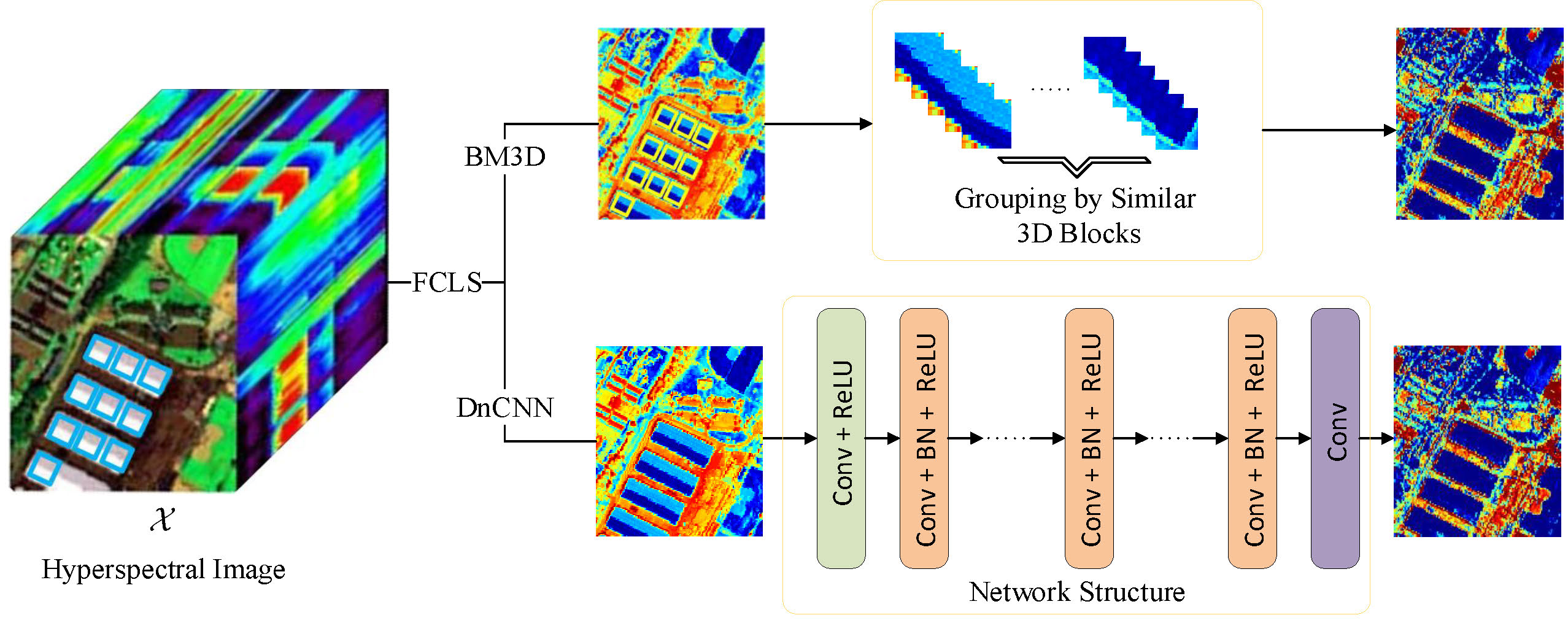
The performance of this method is constrained by the denoiser. Two state-of-the-art denoisers, BM3D and DnCNN, are chosen for the prior information of the abundance maps [43,44]. BM3D is well-known nonlocal patch-based denoiser, which can remove noise in a natural image by taking advantage of high spatial correlation of similar patches in the image. As geographic hyperspectral data, the materials in HSIs tend to be spatially dependent, so it is very easy to find similar patches from the images. Meanwhile, the spatial distribution of a single material tends to be aggregated instead of being purely random. The texture structure of abundance maps can be illustrated with an example given in Figure 1. The unmixing of a San Diego Airport image of size $160\times 140$ pixels was carried out. The first row in Figure 1 shows the abundance map of ‘Ground & road’ estimated by the FCLS [45] followed by an endmember estimation step (vertex component analysis (VCA) [46]). As shown in Figure 1, we can find many similar patches (marked with small yellow squares) from the abundance map. Hence, this nonlocal patch-based denoiser can be used on the abundance maps.

With the development of deep learning, convolutional neural network (CNN) based denoising methods have achieved good results. Specifically, deep network structure can effectively learn the features of images. Hence, in the paper, we also chose a well-known CNN-based denoiser as the prior of the abundance maps, named DnCNN (shown in in Figure 1). DnCNN can handle zero-mean Gaussian noise with unknown standard deviation, and residual learning is adopted to separating noise from noisy observations. Therefore, this method can effectively capture the texture structure of abundance maps.

2.3. Proposed Method: Unmixing with Nonnegative Tensor Factorization and Plug-and-Play Proir

To better represent the structure of abundance maps, mixing model (4) can be equivalently written as

$$\mathcal{Y}=\sum _{i=1}^R{\mathcal{A}}_{:,:,i}\circ {\mathbf{c}}_i+\sum _{j=1}^{R(R-1)/2}{\mathcal{B}}_{:,:,j}\circ {\mathbf{m}}_j+\mathcal{N},$$

(5)

where ${\mathcal{A}}_{:,:,i}\in {\mathbb{R}}^{n_{row}\times n_{col}}$, ${\mathbf{c}}_i\in {\mathbb{R}}^{L\times 1}$, ${\mathcal{B}}_{:,:,j}\in {\mathbb{R}}^{n_{row}\times n_{col}}$, and ${\mathbf{m}}_j\in {\mathbb{R}}^{L\times 1}$ denote the $\mathit{i}$th abundance slice, the $\mathit{i}$th endmember vector, the $\mathit{j}$th interaction abundance slice, and the $\mathit{j}$th interaction endmember vector, respectively. Model (5) is depicted in Figure 2.

To take full advantage of the abundance maps’ prior, we propose a new unmixing method based on the Plug-and-Play (PnP) framework of abundance maps and Nonnegative Tensor Factorization, termed PnP-NTF, which aims to solve the following optimization problem:

$$\begin{array}{c}\underset{j=1,2,...,R(R-1)/2}{\underset{i=1,2,...,R,}{\underset{{\mathcal{A}}_{:,:,i}\ge 0,{\mathcal{B}}_{:,:,j}\ge 0}{argmin}}}\frac{1}{2}{∥\mathcal{Y}-\sum _{i=1}^R{\mathcal{A}}_{:,:,i}\circ {\mathbf{c}}_i-\sum _{j=1}^{R(R-1)/2}{\mathcal{B}}_{:,:,j}\circ {\mathbf{m}}_j∥}_F^2+\sum _{i=1}^R\mathbf{\psi }\left({\mathcal{A}}_{:,:,i}\right)+\sum _{j=1}^{R(R-1)/2}\mathbf{\psi }\left({\mathcal{B}}_{:,:,j}\right)\\ s.t.\sum _{i=1}^R{\mathcal{A}}_{:,:,i}={\mathbf{1}}_{n_{row}}{\mathbf{1}}_{n_{col}}^T,\end{array}$$

(6)

where ${∥\mathcal{X}∥}_F^2$ denotes the Frobenius norm which returns the square root of the sum of the absolute squares of its elements. The symbol $\mathbf{\psi }(.)$ represents the plugged state-of-the-art denoiser, and ${\mathbf{1}}_d$ represents a vector whose components are all one and whose dimension is given by its subscript.

2.4. Optimization Procedure

The optimization problem in (6) can be solved by optimization using the alternating direction method of multipliers (ADMM) [47]. To use the ADMM, first (6) is converted into an equivalent form by introducing multiple auxiliary variables ${\mathbf{V}}_i$, ${\mathbf{E}}_j$ to replace ${\mathcal{A}}_{:,:,i}(i=1,...,R)$, ${\mathcal{B}}_{:,:,j}(j=1,...,R(R-1)/2)$. The formulation is as follows:

$$\begin{array}{c}\underset{{\mathcal{A}}_{:,:,i}\ge 0,{\mathcal{B}}_{:,:,j}\ge 0}{argmin}\frac{1}{2}{∥\mathcal{Y}-\sum _{i=1}^R{\mathcal{A}}_{:,:,i}\circ {\mathbf{c}}_i-\sum _{j=1}^{R(R-1)/2}{\mathcal{B}}_{:,:,j}\circ {\mathbf{m}}_j∥}_F^2+{\lambda }_1\sum _{i=1}^R\mathbf{\psi }\left({\mathbf{V}}_i\right)+{\lambda }_2\sum _{j=1}^{R(R-1)/2}\mathbf{\psi }\left({\mathbf{E}}_j\right)\\ s.t.\left\{\begin{array}{c}{\mathcal{A}}_{:,:,i}={\mathbf{V}}_i,i=1,2,...,R\\ {\mathcal{B}}_{:,:,j}={\mathbf{E}}_j,j=1,2,...,R(R-1)/2\\ \sum _{i=1}^R{\mathcal{A}}_{:,:,i}={\mathbf{1}}_{n_{row}}{\mathbf{1}}_{n_{col}}^T\end{array}\right..\end{array}$$

(7)

By using the Lagrangian function, (7) can be reformulated as:

$$\begin{array}{cc}\hfill & \mathcal{L}({\mathcal{A}}_{:,:,i},{\mathcal{B}}_{:,:,j},{\mathbf{V}}_i,{\mathbf{E}}_j,{\mathbf{D}}_i,{\mathbf{H}}_j,\mathbf{G})=\hfill \\ \hfill & \frac{1}{2}{∥\mathcal{Y}-\sum _{i=1}^R{\mathcal{A}}_{:,:,i}\circ {\mathbf{c}}_i-\sum _{j=1}^{R(R-1)/2}{\mathcal{B}}_{:,:,j}\circ {\mathbf{m}}_j∥}_F^2+{\lambda }_1\sum _{i=1}^R\mathbf{\psi }\left({\mathbf{V}}_i\right)\hfill \\ \hfill & +{\lambda }_2\sum _{j=1}^{R(R-1)/2}\mathbf{\psi }\left({\mathbf{E}}_j\right)+\frac{\mu }{2}(\sum _{i=1}^R{∥{\mathcal{A}}_{:,:,i}-{\mathbf{V}}_i-{\mathbf{D}}_i∥}_F^2)+\hfill \\ \hfill & \frac{\mu }{2}(\sum _{j=1}^{R(R-1)/2}{∥{\mathcal{B}}_{:,:,j}-{\mathbf{E}}_j-{\mathbf{H}}_j∥}_F^2)+\frac{\mu }{2}{∥\sum _{i=1}^R{\mathcal{A}}_{:,:,i}-{\mathbf{1}}_{n_{row}}{\mathbf{1}}_{n_{col}}^T-\mathbf{G}∥}_F^2,\hfill \end{array}$$

(8)

where ${\mathbf{D}}_i$, ${\mathbf{H}}_j$ and $\mathbf{G}$ are scaled dual variables [48], and $\mu$ is the penalty parameter. The variables ${\mathcal{A}}_{:,:,i},{\mathcal{B}}_{:,:,j},{\mathbf{V}}_i,{\mathbf{E}}_j,{\mathbf{D}}_i,{\mathbf{H}}_j,\mathbf{G}$ were updated sequentially: this step is shown in Algorithm 1. The solution of optimization is detailed below.

Algorithm 1:The Proposed PnP-NTF Unmixing Method.

• Updating of $\mathcal{A}$
  The optimization problem for ${\mathcal{A}}_{:,:,i}$ is

  $$\begin{array}{cc}\hfill & {\mathcal{A}}_{:,:,i}^{k+1}=\underset{{\mathcal{A}}_{:,:,i}^k}{argmin}\frac{1}{2}{∥\mathcal{Y}-\sum _{i=1}^R{\mathcal{A}}_{:,:,i}^k\circ {\mathbf{c}}_i-\sum _{j=1}^{R(R-1)/2}{\mathcal{B}}_{:,:,j}^k\circ {\mathbf{m}}_j∥}_F^2\hfill \\ \hfill & +\frac{\mu }{2}{∥{\mathcal{A}}_{:,:,i}^k-{\mathbf{V}}_i^k-{\mathbf{D}}_i^k∥}_F^2+\frac{\mu }{2}{∥\sum _{i=1}^R{\mathcal{A}}_{:,:,i}^k-{\mathbf{1}}_{n_{row}}{\mathbf{1}}_{n_{col}}^T-{\mathbf{G}}^k∥}_F^2\hfill \\ \hfill & =\frac{1}{2}\sum _{b=1}^L{∥{\mathcal{O}}_{:,:,b}-{\mathcal{A}}_{:,:,i}^k{\mathit{c}}_{i_b}∥}_F^2+\frac{\mu }{2}(\sum _{i=1}^R{∥{\mathcal{A}}_{:,:,i}^k-{\mathbf{V}}_i^k-{\mathbf{D}}_i^k∥}_F^2)\hfill \\ \hfill & +\frac{\mu }{2}{∥{\mathcal{A}}_{:,:,i}^k+\tilde{\mathbf{A}}-{\mathbf{1}}_{n_{row}}{\mathbf{1}}_{n_{col}}^T-{\mathbf{G}}^k∥}_F^2,\hfill \end{array}$$

  (9)

  where $\mathcal{O}=\mathcal{Y}-\sum _{i=1,\neg i}^R{\mathcal{A}}_{:,:,i}^k\circ {\mathbf{c}}_i-\sum _{j=1}^{R(R-1)/2}{\mathcal{B}}_{:,:,j}^k\circ {\mathbf{m}}_j\in {\mathbb{R}}^{n_{row}\times n_{col}\times L}$, and ${\mathcal{O}}_{:,:,b}$ is the bth slice. Meanwhile, $\tilde{\mathbf{A}}=\sum _{i=1,\neg i}^R{\mathcal{A}}_{:,:,i}^k\in {\mathbb{R}}^{n_{row}\times n_{col}}$ and ${\mathbf{c}}_i={[{\mathit{c}}_{i_1},{\mathit{c}}_{i_2}...,{\mathit{c}}_{i_b},...,{\mathit{c}}_{i_L}]}^{\mathit{T}}\in {\mathbb{R}}^{L\times 1}$ is the ith endmember. Hence the solution for ${\mathcal{A}}_{:,:,i}$ can be derived as follows:

  $$\begin{array}{ccc}\hfill & {\mathcal{A}}_{:,:,i}^{k+1}=\hfill & \hfill {(\sum _{b=1}^L{\mathit{c}}_{i_b}{\mathit{c}}_{i_b}^T+2\mu \mathbf{I})}^{-1}(\sum _{b=1}^B{\mathcal{O}}_{:,:b}{\mathit{c}}_{i_b}^T+\mu ({\mathbf{V}}_i^k+{\mathbf{D}}_i^k+{\mathbf{1}}_{n_{row}}{\mathbf{1}}_{n_{col}}^T+{\mathbf{G}}^k-\tilde{\mathbf{A}})).\end{array}$$

  (10)
• Updating of $\mathcal{B}$
  The optimization problem for ${\mathcal{B}}_{:,:,j}$ is

  $$\begin{array}{ccc}\hfill {\mathcal{B}}_{:,:,j}^{k+1}& =\underset{{\mathcal{B}}_{:,:,j}^k}{argmin}\frac{1}{2}{∥\mathcal{Y}-\sum _{i=1}^R{\mathcal{A}}_{:,:,i}^{k+1}\circ {\mathbf{c}}_i-\sum _{j=1}^{R(R-1)/2}{\mathcal{B}}_{:,:,j}^k\circ {\mathbf{m}}_j∥}_F^2\hfill & \hfill +\frac{\mu }{2}{∥{\mathcal{B}}_{:,:,j}^k-{\mathbf{E}}_j^k-{\mathbf{H}}_j^k∥}_F^2\\ \hfill & =\frac{1}{2}\sum _{b=1}^L{∥{\mathcal{K}}_{:,:,b}-{\mathcal{B}}_{:,:,j}^k{\mathit{m}}_{j_b}∥}_F^2+\frac{\mu }{2}{∥{\mathcal{B}}_{:,:,j}^k-{\mathbf{E}}_j^k-{\mathbf{H}}_j^k∥}_F^2,\hfill \end{array}$$

  (11)

  where $\mathcal{K}=\mathcal{Y}-\sum _{i=1}^R{\mathcal{A}}_{:,:,i}^k\circ {\mathbf{c}}_i-\sum _{j=1,,\neg j}^{R(R-1)/2}{\mathcal{B}}_{:,:,j}^k\circ {\mathbf{m}}_j\in {\mathbb{R}}^{n_{row}\times n_{col}\times L}$, and ${\mathcal{K}}_{:,:,b}$ is the bth slice. Meanwhile, ${\mathbf{m}}_j={[{\mathit{m}}_{j_1},{\mathit{m}}_{j_2}...,{\mathit{m}}_{j_b},...,{\mathit{m}}_{j_L}]}^{\mathit{T}}\in {\mathbb{R}}^{L\times 1}$ is the jth interaction endmember. Hence the solution for ${\mathcal{B}}_{:,:,j}$ can be derived as follows:

  $$\begin{array}{cc}\hfill {\mathcal{B}}_{:,:,j}^{k+1}& ={(\sum _{b=1}^L{\mathit{m}}_{j_b}{\mathit{m}}_{j_b}^T+\mu \mathbf{I})}^{-1}(\sum _{b=1}^L{\mathcal{K}}_{:,:,b}{\mathit{m}}_{j_b}^T+\mu ({\mathbf{E}}_j^k+{\mathbf{H}}_j^k)).\hfill \end{array}$$

  (12)
• Updating of $\mathbf{V}$
  The optimization problem for ${\mathbf{V}}_i$ is

  $$\begin{array}{cc}\hfill {\mathbf{V}}_i^{k+1}& =\underset{{\mathbf{V}}_i^k}{argmin}{\lambda }_1\mathbf{\psi }\left({\mathbf{V}}_i^k\right)+\frac{\mu }{2}{∥{\mathcal{A}}_{:,:,i}^{k+1}-{\mathbf{V}}_i^k-{\mathbf{D}}_i^k∥}_F^2\hfill \\ \hfill & =\frac{1}{2}{∥{\tilde{\mathbf{V}}}_i-{\mathbf{V}}_i^k∥}_F^2+\frac{{\lambda }_1}{\mu }\mathbf{\psi }\left({\mathbf{V}}_i^k\right),\hfill \end{array}$$

  (13)

  where ${\tilde{\mathbf{V}}}_i={\mathcal{A}}_{:,:,i}^{k+1}-{\mathbf{D}}_i^k\in {\mathbb{R}}^{n_{row}\times n_{col}}$. Sub-problem (13) can be solved using PnP framework of ${\tilde{\mathbf{V}}}_i$, then ${\mathbf{V}}_i^{k+1}$ can be calculated as

  $${\mathbf{V}}_i^{k+1}=\mathbf{PnP}\left({\tilde{\mathbf{V}}}_i\right).$$

  (14)
• Updating of $\mathbf{E}$
  The optimization problem for ${\mathbf{E}}_j$ is

  $$\begin{array}{cc}\hfill {\mathbf{E}}_j^{k+1}& =\underset{{\mathbf{E}}_j^k}{argmin}{\lambda }_2\mathbf{\psi }\left({\mathbf{E}}_j\right)+\frac{\mu }{2}{∥{\mathcal{B}}_{:,:,j}^{k+1}-{\mathbf{E}}_j^k-{\mathbf{H}}_j^k∥}_F^2\hfill \\ \hfill & =\frac{1}{2}{∥{\tilde{\mathbf{E}}}_j-{\mathbf{E}}_j^k∥}_F^2+\frac{{\lambda }_2}{\mu }\mathbf{\psi }\left({\mathbf{E}}_j\right),\hfill \end{array}$$

  (15)

  where ${\tilde{\mathbf{E}}}_j={\mathcal{B}}_{:,:,j}^{k+1}-{\mathbf{H}}_j^k\in {\mathbb{R}}^{n_{row}\times n_{col}}$. Sub-problem (15) can be solved via PnP framework of ${\tilde{\mathbf{E}}}_j$, then ${\mathbf{E}}_j^{k+1}$ can be expressed as

  $${\mathbf{E}}_j^{k+1}=\mathbf{PnP}\left({\tilde{\mathbf{E}}}_j\right).$$

  (16)
• Updating of $\mathbf{D}$

  $${\mathbf{D}}_i^{k+1}={\mathbf{D}}_i^k-({\mathcal{A}}_{:,:,i}^{k+1}-{\mathbf{V}}_i^{k+1}).$$

  (17)
• Updating of $\mathbf{H}$

  $${\mathbf{H}}_j^{k+1}={\mathbf{H}}_j^k-({\mathcal{B}}_{:,:,j}^{k+1}-{\mathbf{E}}_j^{k+1}).$$

  (18)
• Updating of G

  $${\mathbf{G}}^{k+1}={\mathbf{G}}^k-(\sum _{i=1}^R{\mathcal{A}}_{:,:,i}^{k+1}-{\mathbf{1}}_{n_{row}}{\mathbf{1}}_{n_{col}}^T).$$

  (19)

3. Experiments and Analysis on Synthetic Data

In this section, we illustrate the performance of the proposed PnP-NTF framework on the two state-of-the-art denoising method, named BM3D and DnCNN, for the abundance estimation. We compare the proposed method with some advanced algorithms to address the GBM, which contains gradient descent algorithm (GDA) [49], the semi-nonnegative matrix factorization (semi-NMF) [50] algorithm and subspace unmixing with low-rank attribute embedding algorithm (SULoRA) [11]. For specifically, the GDA method is a benchmark to solve the GBM pixel by pixel, and semi-NMF can speed up and reduce the time loss. Meanwhile, the semi-NMF based method can consider the partial spatial information of the image. SULoRA is a general subspace unmixing method that jointly estimates subspace projections and abundance, and can model the raw subspace with low-rank attribute embedding. All of the experiments were conducted in MATLAB R2018b on a desktop of 16 GB RAM, Intel (R) Core (TM) i5-8400 CPU, @2.80 GHz.

In order to quantify the effect of the proposed method numerically, three widely metrics, including the root-mean-square error (RMSE) of abundances, the image reconstruction error (RE), and the average of spectral angle mapper (aSAM) are used. For specifically, the RMSE quantifies the difference between the estimated abundance $\widehat{\mathcal{A}}$ and the true abundances $\mathcal{A}$ as follows:

$$\mathit{RMSE}=\sqrt{\frac{1}{R\times N}{\parallel \mathcal{A}-\widehat{\mathcal{A}}\parallel }_F^2}.$$

(20)

The RE measures the difference between the observation $\mathcal{Y}$ and its reconstruction $\widehat{\mathcal{Y}}$ as follows:

$$\mathit{RE}=\sqrt{\frac{1}{N\times L}{\parallel \mathcal{Y}-\widehat{\mathcal{Y}}\parallel }_F^2}.$$

(21)

The aSAM qualifies the average spectral angle mapping of the estimated ith spectral vector ${\widehat{\mathbf{y}}}_l$ and observed ith spectral vector $\mathbf{y}$. The aSAM is defined as follows:

$$aSAM=\frac{1}{N}\sum _{i=1}^{N}arccos\left(\frac{{\mathbf{y}}_i^{\mathrm{T}}·{\widehat{\mathbf{y}}}_i}{∥{\mathbf{y}}_i∥∥{\widehat{\mathbf{y}}}_i∥}\right).$$

(22)

3.1. Data Generation

In the simulated experiments, the synthetic data was generated similar to References [32,51], and the specific process is as follows:

• Six spectral endmembers signals with 224 spectral bands were randomly chosen from the USGS digital spectral library (https://www.usgs.gov/labs/spec-lab), namely Carnallite, Ammonio–jarosite, Almandine, Brucite, Axinite, and Chlonte.
• We generated a simulated image of size $s^2\left(\mathrm{rows}\right)\times s^2\left(\mathrm{columns}\right)\times L\left(\mathrm{bands}\right)$, which can be divided into small blocks of size $s\times s\times L$.
• A randomly selected endmember was assigned to each block, and a $k\times k$ low-pass filter was used to generate abundance map cube of size $s^2\times s^2\times R$ that contained mixed pixels, while satisfying the ANC and ASC constraints.
• After obtaining the endmember information and the abundance information, then clean HSIs can be generated by the generalized bilinear model and the polynomial post nonlinear model. The interaction coefficient parameters in the GBM were set randomly, and the nonlinear coefficient parameters in the PPNM were set to 0.25.
• To effectively evaluate the robustness performance of the proposed method on the different signal-to-noise ratio (SNR), the zero-mean Gaussian white noise was added to the clean data.

3.2. Evaluation of the Methods

The details of the simulated data can be obtained with the previous steps, then we generated a series of noisy images with SNRs = {15, 20, 30} dB to evaluate performance of the proposed method and compare with other methods.

3.2.1. Parameter Setting

To compare all the algorithms fairly, the parameters in the all compared methods were hand-tuned to the optimal values. Specifically, the FCLS was used to initialize the abundance information in the all methods (including the proposed method). Note that a direct compasion with FCLS unmixing results is unfair and FCLS is served as a benchmark, which shows the impact of using a linear unmixing method on nonlinear mixed images. The GDA is considered as the benchmark to solve the GBM. The tolerances for stopping the iterations in GDA, Semi-NMF, and SULoRA were set to $1\times {10}^{-6}$. For the proposed PnP-NTF framework based method, the parameters to be adjusted were divided into two parts, one of which is the parameter of the denoiser we chosen, and the other part is the penalty parameter $\mu$. Firstly, the standard deviation of additive white Gaussian noise $\sigma$ is searching from 0 to 255 with the step of 25, the the block size used for the hard-thresholding (HT) filtering is set as 8 in BM3D, respectively. The parameters of the DnCNN is the same as Reference [44]. Meanwhile, the penalty parameter $\mu$ was set to $8\times {10}^{-3}$, and the tolerance for stopping the iterations was set to $1\times {10}^{-6}$.

3.2.2. Comparison of Methods under Different Gaussian Noise Levels

In our experiments, we generate three images of size $64\times 64\times 224$ with 4096 pixels and 224 bands. More specifically, the ‘Scene1’ is generated by the GBM model, and the ‘Scene2’ is generated by the PPNM model. The ‘Scene3’ is a mixture of the ‘Scene1’ and ‘Scene2’, as half pixels in ‘Scene3’ were generated by the GBM and the others were generated by PPNM [50]. The ‘Scene1’ is used to evaluate the efficiency of the proposed method to handle mixtures based on GBM, while the ‘Scene2’ and ‘Scene3’ were used to evaluate the robustness of the proposed method to mixtures based on different mixing models.

For the proposed method and the other methods, the abundances were initialized with the same method, that is FCLS. In a supervised nonlinear unmixing problem, the spectral vectors of endmember were known as a priori. Considering that the accuracy of abundance inversion depends on the quality of endmember signals, we used the true endmembers in the experiments for fair comparison.

Table 1. Evaluation Results in ’Scene1’ with different signal-to-noise ratios (SNRs) and time cost (s).

Scenario	SNR (dB)	Metric	FCLS	GDA	Semi-NMF	SULoRA	PnP-NTF-BM3D (Proposed)	PnP-NTF-DnCNN (Proposed)
Scene1’	15	RMSE	0.0614	0.0535	0.0521	0.0521	0.0431	0.0428
		RE	0.0898	0.0893	0.0879	0.0879	0.0876	0.0876
		aSAM	0.1773	0.1764	0.1744	0.1743	0.1737	0.1737
		Time	1	590	6	1	700	450
	20	RMSE	0.0544	0.0449	0.0405	0.0372	0.0269	0.0267
		RE	0.0527	0.0519	0.0497	0.0497	0.0492	0.0492
		aSAM	0.1039	0.1024	0.0991	0.0991	0.0982	0.0982
		Time	1	609	7	1	839	585
	30	RMSE	0.0511	0.0409	0.0315	0.0265	0.0125	0.0125
		RE	0.0242	0.0224	0.0167	0.0171	0.0156	0.0156
		aSAM	0.0447	0.0411	0.0330	0.0329	0.0312	0.0312
		Time	1	611	13	1	1142	836

quantifies the corresponding results of the three evaluation indicators (RMSE, RE, and aSAM) in detail on the ‘Scene1’. As seen from the Table 1, the proposed PnP-NTF based framework with the advanced denoisers provide the superior unmixing results, compared with other methods. Specifically, we tested two state-of-the-art denoisers, namely BM3D and DnCNN, and both of them obtained the best performance. The RMSE, RE, and aSAM obtained minimum values from the proposed PnP-NTF based frameworks, which show the efficiency of the proposed methods is superior compared with other state-of-the-art methods (shown in bold). Figure 3 shows the results of the proposed algorithm and the others algorithms under three indexes (RMSE, RE, and aSAM). For the different levels of noise in ‘Scene1’, the proposed methods yield the superior performance in all indexes. Also we can see from the histogram of Figure 4, Figure 5 and Figure 6 that the proposed methods obtain the minimum RMSEs in all scenes.

To evaluate the robustness of the proposed methods against model error, we generated ‘Scene2’ and ‘Scene3’ of size $64\times 64\times 224$. As shown in

Table 2. Evaluation Results in ’Scene2’ with different SNRs and time cost (s).

Scenario	SNR (dB)	Metric	FCLS	GDA	Semi-NMF	SULoRA	PnP-NTF-BM3D (Proposed)	PnP-NTF-DnCNN (Proposed)
Scene2’	15	RMSE	0.0804	0.0683	0.0586	0.0596	0.0437	0.0434
		RE	0.0956	0.0946	0.0919	0.0918	0.0913	0.0913
		aSAM	0.1805	0.1787	0.1748	0.1746	0.1737	0.1737
		Time	1	557	8	1	712	465
	20	RMSE	0.0759	0.0626	0.0487	0.0461	0.0281	0.0280
		RE	0.0582	0.0566	0.0523	0.0521	0.0514	0.0514
		aSAM	0.1092	0.1063	0.1000	0.0998	0.0984	0.0984
		Time	1	564	11	1	687	452
	30	RMSE	0.0738	0.0601	0.0396	0.0370	0.0167	0.0167
		RE	0.0314	0.0285	0.0183	0.0206	0.0163	0.0163
		aSAM	0.0558	0.0491	0.0345	0.0381	0.0314	0.0314
		Time	1	561	18	1	795	603

and

Table 3. Evaluation Results in ’Scene3’ with different SNRs and time cost (s).

Scenario	SNR (dB)	Metric	FCLS	GDA	Semi-NMF	SULoRA	PnP-NTF-BM3D (Proposed)	PnP-NTF-DnCNN (Proposed)
Scene3’	15	RMSE	0.0745	0.0649	0.0577	0.0565	0.0433	0.0430
		RE	0.0934	0.0927	0.0905	0.0903	0.0899	0.0899
		aSAM	0.1790	0.1778	0.1748	0.1747	0.1739	0.1739
		Time	1	544	7	1	649	420
	20	RMSE	0.0692	0.0583	0.0470	0.0417	0.0280	0.0279
		RE	0.0559	0.0548	0.0513	0.0511	0.0504	0.0504
		aSAM	0.1061	0.1042	0.0995	0.0993	0.0982	0.0982
		Time	1	573	9	1	712	472
	30	RMSE	0.0665	0.0552	0.0382	0.0319	0.0150	0.0151
		RE	0.0284	0.0262	0.0178	0.0187	0.0160	0.0160
		aSAM	0.0493	0.0447	0.0338	0.0354	0.0312	0.0312
		Time	1	572	16	1	957	664

, the proposed methods obtained the best estimate of abundances in terms of RMSE, RE, and aSAM (shown in bold). We cannot provide the proof of the convergence of the proposed algorithm, but the experimental results show that it is convergent when plugged by BM3D and DnCNN (shown in Figure 7 and Figure 8).

3.2.3. Comparison of Methods under Denoised Abundance Maps

We make a series of experiments to show the difference between the proposed methods and the conventional unmixing methods (FCLS, GDA, and Semi-NMF) with afterwards denoising the calculated abundance maps by BM4D. The results in

Table 4. Evaluation result of denoised abundance in ’Scene1’ with different SNRs.

Scenario	SNR (dB)	Metric	FCLS Denoised	GDA Denoised	Semi-NMF Denoised	PnP-NTF-BM3D (Proposed)	PnP-NTF-DnCNN (Proposed)
Scene1’	15	RMSE	0.0501	0.0408	0.0369	0.0431	0.0428
	20		0.0489	0.0388	0.0328	0.0269	0.0267
	30		0.0487	0.0383	0.0283	0.0125	0.0125

,

Table 5. Evaluation result of denoised abundance in ’Scene2’ with different SNRs.

Scenario	SNR (dB)	Metric	FCLS Denoised	GDA Denoised	Semi-NMF Denoised	PnP-NTF-BM3D (Proposed)	PnP-NTF-DnCNN (Proposed)
Scene2’	15	RMSE	0.0734	0.0599	0.0446	0.0437	0.0434
	20		0.0733	0.0593	0.0423	0.0281	0.0280
	30		0.0734	0.0594	0.0376	0.0167	0.0167

and

Table 6. Evaluation result of denoised abundance in ’Scene3’ with different SNRs.

Scenario	SNR (dB)	Metric	FCLS Denoised	GDA Denoised	Semi-NMF Denoised	PnP-NTF-BM3D (Proposed)	PnP-NTF-DnCNN (Proposed)
Scene3’	15	RMSE	0.0665	0.0557	0.0435	0.0433	0.0430
	20		0.0659	0.0545	0.0404	0.0280	0.0279
	30		0.0656	0.0542	0.0360	0.0150	0.0151

show that the denoised abundance maps provided by FCLS, GDA, and Semi-NMF can obtain a better results than corresponding original abundance maps. However, for the proposed methods, we use directly a state-of-the-art denoiser as the regularization, which is to exploit the spatial correlation of abundance maps. The results show that using plug-and-play prior for the abundance maps and interaction abundance maps can enhance the accuracy of the estimated abundance results efficiently.

4. Experiments and Analysis on Real Dataset

In this section, we use two real hyperspectral datasets to validate the performance of the proposed methods. Due to the lack of the groundtruth of abundances in the real scenes, the RE in (21) and the aSAM in (22) were used to test the unmixing performance of the all methods. The convergence of the proposed methods on the two real hyperspectral datasets are shown in Figure 9.

4.1. San Diego Airport

The first real dataset is called ‘San Diego Airport’ image, which was captured by the AVIRIS over San Diego. The original image of size $400\times 400$ includes 224 spectral channels in the wavelength range of 370 nm to 2510 nm. After removing bands affected by water vapor absorption, 189 band are kept. For our experiments, a subimage of size 160 (rows)$\times 140$ (columns) (shown in Figure 10a) is chosen as the test image. The selected scene mainly contains five endmembers, namely ‘Roof’, ‘Grass’, ‘Rround and Road’, ‘Tree’, and ‘Other’ [52].

The subimage we chosen has been studied in Reference [52]. VCA [46] method is used to estiamte the endmebers. Meanwhile, the FCLS is used to initialize the abundances in all methods. The ASC constraint in the semi-NMF was set to 0.1. Two state-of-the-art denoisers, embedded in the proposed PnP-NTF-based framework were tested. For the BM3D denoiser, the standard deviation of noise was hand-tuned. For the DnCNN denoiser, its parameter was set in a same way as Reference [44]. The penalty parameter $\mu$ was set to $1\times {10}^{-4}$. The tolerance for stopping the iterations was set to $1\times {10}^{-6}$ for all algorithms.

Table 7. Evaluation Results with the RE, aSAM and cost time (s) on the San Diego Airport.

Scenario	Metric	FCLS	GDA	SULoRA	Semi-NMF	PnP-NTF-BM3D (Proposed)	PnP-NTF-DnCNN (Proposed)
San Diego Airport	RE	0.0165	0.0164	0.0156	0.0150	0.0132	0.0131
	aSAM	0.0596	0.0594	0.0535	0.0542	0.0455	0.0454
	Time	5	168	4	47	191	108

shows the performance of different unmixing methods in terms of RE and aSAM in the San Diego Airport image. Our proposed method obtains the best results. Figure 11 shows the estimated abundance maps obtained by all methods. Focusing on the abundance maps of ‘Ground and Road’, we can see that the roof area is regarded as a mixture of ‘Roof’ and ‘Ground and Road’ in the unmixing results of FCLS, GDA, Semi-NMF and SULoRA methods. In fact, the the roof area only contains endmember ‘Roof’. Unmixing results of the proposed PnP-NTF-DnCNN/BM3D are more reasonable.

Furthermore, Figure 12 shows the distribution of the RE on the San Diego Airport. The bright areas in Figure 12 indicate large errors in the reconstructed images. The error map shows that the FCLS performed worst, because the FCLS only can handle the linear information but ignore the nonlinear information in the image. Meanwhile, the semi-NMF performed better than GDA because the GDA is a pixel-based algorithm that does not take any spatial information into consideration. Our method, exploiting self-similarity of abundance maps, can perform better than other methods.

4.2. Washington DC Mall

The second real dataset is called ‘Washington DC Mall’ image, which was acquired by HYDICE sensor over Washington DC, USA. The original image of size $1208\times 307$ includes 210 spectral bands. Its spatial resolution is 3 m. After removing bands corrupted by water vapor absorption, 191 band are kept. There are seven endmembers in the image: ‘Roof’, ‘Grass’, ‘Road’, ‘Trail’, ‘Water’, ‘Shadow’, and ‘Tree’ [52]. We chose a subimage with $256\times 256$ pixels for the experiments, called sub-DC (shown in Figure 10b). The Hysime [53] was firstly used to estimate the number of endmembers, then the VCA was used to extract the spectral information of endmembers. The extracted endmembers were named ‘Roof1’, ‘Roof2’, ‘Grass’, ‘Road’, ‘Tree’, and ‘Trail’.

The parameters in the comparison methods were manually tuned to obtain optimal performance. The parameter setting of our methods was same as that in the ‘San Diego Airport’ image.

Table 8. Evaluation Results with the RE, aSAM and cost time (s) on the Washington DC Mall.

Scenario	Metric	FCLS	GDA	SULoRA	Semi-NMF	PnP-NTF-BM3D (Proposed)	PnP-NTF-DnCNN (Proposed)
Washington DC Mall	RE	0.0156	0.0154	0.0152	0.0120	0.0099	0.0099
	aSAM	0.1020	0.1015	0.0880	0.0837	0.0623	0.0621
	Time	17	670	10	43	1163	585

shows the results of the proposed method and the state-of-the-art methods in the ‘Washington DC Mall’ image. The proposed methods obtained the best results in terms of RE and aSAM. Figure 13 and Figure 14 show the estimated abundance maps and the error maps, respectively. In Figure 14, the proposed methods show much smaller errors in the reconstructed images.

5. Conclusions

In this paper, we propose a new hyperspectral nonlinear unmixing framework, which takes advantage of spatial correlation (i.e., self-similarity) of abundance maps through a plug-and-play technique. The self-similarity of abundance maps is imposed on our objective function, which is solved by ADMM embedded with a denoising method based regularization. We tested two state-of-the-art denoising methods (BM3D and DnCNN). In the experiments with simulated data and real data, the proposed methods can obtain more accurate estimation of abundances than state-of-the-art methods. Furthermore, we tested the proposed method in case of the number of endmembers with 5, and obtained better results compared to other methods. However, with the growing of the number of endmembers, the difficulty of unmixing will also increase, which is our future research direction.

References

- Dobigeon, N.; Tourneret, J.; Richard, C.; Bermudez, J.C.M.; McLaughlin, S.; Hero, A.O. Nonlinear Unmixing of Hyperspectral Images: Models and Algorithms. IEEE Signal Process. Mag. 2014, 31, 82–94. [Google Scholar] [CrossRef] [Green Version]
- Keshava, N.; Mustard, J.F. Spectral unmixing. IEEE Signal Process. Mag. 2002, 19, 44–57. [Google Scholar] [CrossRef]
- Bioucas-Dias, J.M.; Plaza, A.; Dobigeon, N.; Parente, M.; Du, Q.; Gader, P.; Chanussot, J. Hyperspectral Unmixing Overview: Geometrical, Statistical, and Sparse Regression-Based Approaches. IEEE J. Sel. Top. Appl. Earth Obs. Remote Sens. 2012, 5, 354–379. [Google Scholar] [CrossRef] [Green Version]
- Zhang, T.-t.; Liu, F. Application of hyperspectral remote sensing in mineral identification and mapping. In Proceedings of the 2012 2nd International Conference on Computer Science and Network Technology, Changchun, China, 29–31 December 2012; pp. 103–106. [Google Scholar] [CrossRef]
- Contreras, C.; Khodadadzadeh, M.; Tusa, L.; Loidolt, C.; Tolosana-Delgado, R.; Gloaguen, R. Geochemical And Hyperspectral Data Fusion For Drill-Core Mineral Mapping. In Proceedings of the 2019 10th Workshop on Hyperspectral Imaging and Signal Processing: Evolution in Remote Sensing (WHISPERS), Amsterdam, The Netherlands, 24–26 September 2019; pp. 1–4. [Google Scholar] [CrossRef]
- Marinoni, A.; Clenet, H. Identification of mafic minerals on Mars by nonlinear hyperspectral unmixing. In Proceedings of the 2016 8th Workshop on Hyperspectral Image and Signal Processing: Evolution in Remote Sensing (WHISPERS), Los Angeles, CA, USA, 21–24 August 2016; pp. 1–4. [Google Scholar] [CrossRef]
- Huang, Z.; Zheng, J. Extraction of Black and Odorous Water Based on Aerial Hyperspectral CASI Image. In Proceedings of the IGARSS 2019—2019 IEEE International Geoscience and Remote Sensing Symposium, Yokohama, Japan, 28 July–2 August 2019; pp. 6907–6910. [Google Scholar] [CrossRef]
- Li, Q.; Kit Wong, F.K.; Fung, T. Comparison Feature Selection Methods for Subtropical Vegetation Classification with Hyperspectral Data. In Proceedings of the IGARSS 2019—2019 IEEE International Geoscience and Remote Sensing Symposium, Yokohama, Japan, 28 July–2 August 2019; pp. 3693–3696. [Google Scholar] [CrossRef]
- Yu, H.; Gao, L.; Liao, W.; Zhang, B.; Zhuang, L.; Song, M.; Chanussot, J. Global Spatial and Local Spectral Similarity-Based Manifold Learning Group Sparse Representation for Hyperspectral Imagery Classification. IEEE Trans. Geosci. Remote Sens. 2020, 58, 3043–3056. [Google Scholar] [CrossRef]
- Zhang, B.; Zhuang, L.; Gao, L.; Luo, W.; Ran, Q.; Du, Q. PSO-EM: A Hyperspectral Unmixing Algorithm Based On Normal Compositional Model. IEEE Trans. Geosci. Remote Sens. 2014, 52, 7782–7792. [Google Scholar] [CrossRef]
- Hong, D.; Zhu, X.X. SULoRA: Subspace Unmixing With Low-Rank Attribute Embedding for Hyperspectral Data Analysis. IEEE J. Sel. Top. Signal Process. 2018, 12, 1351–1363. [Google Scholar] [CrossRef]
- Zhuang, L.; Lin, C.; Figueiredo, M.A.T.; Bioucas-Dias, J.M. Regularization Parameter Selection in Minimum Volume Hyperspectral Unmixing. IEEE Trans. Geosci. Remote Sens. 2019, 57, 9858–9877. [Google Scholar] [CrossRef]
- Qu, Y.; Qi, H. uDAS: An Untied Denoising Autoencoder With Sparsity for Spectral Unmixing. IEEE Trans. Geosci. Remote Sens. 2019, 57, 1698–1712. [Google Scholar] [CrossRef]
- Hong, D.; Yokoya, N.; Chanussot, J.; Zhu, X.X. An Augmented Linear Mixing Model to Address Spectral Variability for Hyperspectral Unmixing. IEEE Trans. Image Process. 2019, 28, 1923–1938. [Google Scholar] [CrossRef] [Green Version]
- Halimi, A.; Altmann, Y.; Dobigeon, N.; Tourneret, J. Nonlinear Unmixing of Hyperspectral Images Using a Generalized Bilinear Model. IEEE Trans. Geosci. Remote Sens. 2011, 49, 4153–4162. [Google Scholar] [CrossRef] [Green Version]
- Altmann, Y.; Halimi, A.; Dobigeon, N.; Tourneret, J. Supervised Nonlinear Spectral Unmixing Using a Postnonlinear Mixing Model for Hyperspectral Imagery. IEEE Trans. Image Process. 2012, 21, 3017–3025. [Google Scholar] [CrossRef] [PubMed] [Green Version]
- Heylen, R.; Scheunders, P. A Multilinear Mixing Model for Nonlinear Spectral Unmixing. IEEE Trans. Geosci. Remote Sens. 2016, 54, 240–251. [Google Scholar] [CrossRef]
- Marinoni, A.; Plaza, J.; Plaza, A.; Gamba, P. Estimating Nonlinearities in p-Linear Hyperspectral Mixtures. IEEE Trans. Geosci. Remote Sens. 2018, 56, 6586–6595. [Google Scholar] [CrossRef]
- Tang, M.; Zhang, B.; Marinoni, A.; Gao, L.; Gamba, P. Multiharmonic Postnonlinear Mixing Model for Hyperspectral Nonlinear Unmixing. IEEE Geosci. Remote Sens. Lett. 2018, 15, 1765–1769. [Google Scholar] [CrossRef]
- Zhu, F.; Honeine, P.; Chen, J. Pixel-Wise Linear/Nonlinear Nonnegative Matrix Factorization for Unmixing of Hyperspectral Data. In Proceedings of the ICASSP 2020—2020 IEEE International Conference on Acoustics, Speech and Signal Processing (ICASSP), Barcelona, Spain, 4–8 May 2020; pp. 4737–4741. [Google Scholar] [CrossRef]
- Zhang, S.; Li, J.; Li, H.; Deng, C.; Plaza, A. Spectral–Spatial Weighted Sparse Regression for Hyperspectral Image Unmixing. IEEE Trans. Geosci. Remote Sens. 2018, 56, 3265–3276. [Google Scholar] [CrossRef]
- Patel, J.R.; Joshi, M.V.; Bhatt, J.S. Abundance Estimation Using Discontinuity Preserving and Sparsity-Induced Priors. IEEE J. Sel. Top. Appl. Earth Obs. Remote Sens. 2019, 12, 2148–2158. [Google Scholar] [CrossRef]
- Zhang, L.; Wei, W.; Zhang, Y.; Yan, H.; Li, F.; Tian, C. Locally Similar Sparsity-Based Hyperspectral Compressive Sensing Using Unmixing. IEEE Trans. Comput. Imaging 2016, 2, 86–100. [Google Scholar] [CrossRef]
- Drumetz, L.; Meyer, T.R.; Chanussot, J.; Bertozzi, A.L.; Jutten, C. Hyperspectral Image Unmixing with Endmember Bundles and Group Sparsity Inducing Mixed Norms. IEEE Trans. Image Process. 2019, 28, 3435–3450. [Google Scholar] [CrossRef]
- Qu, Q.; Nasrabadi, N.M.; Tran, T.D. Abundance Estimation for Bilinear Mixture Models via Joint Sparse and Low-Rank Representation. IEEE Trans. Geosci. Remote Sens. 2014, 52, 4404–4423. [Google Scholar] [CrossRef]
- Giampouras, P.V.; Themelis, K.E.; Rontogiannis, A.A.; Koutroumbas, K.D. Simultaneously Sparse and Low-Rank Abundance Matrix Estimation for Hyperspectral Image Unmixing. IEEE Trans. Geosci. Remote Sens. 2016, 54, 4775–4789. [Google Scholar] [CrossRef] [Green Version]
- Feng, F.; Zhao, B.; Tang, L.; Wang, W.; Jia, S. Robust low-rank abundance matrix estimation for hyperspectral unmixing. J. Eng. 2019, 2019, 7406–7409. [Google Scholar] [CrossRef]
- Li, H.; Feng, R.; Wang, L.; Zhong, Y.; Zhang, L. Superpixel-Based Reweighted Low-Rank and Total Variation Sparse Unmixing for Hyperspectral Remote Sensing Imagery. IEEE Trans. Geosci. Remote. Sens. 2020, 1–19. [Google Scholar] [CrossRef]
- Feng, X.; Li, H.; Li, J.; Du, Q.; Plaza, A.; Emery, W.J. Hyperspectral Unmixing Using Sparsity-Constrained Deep Nonnegative Matrix Factorization With Total Variation. IEEE Trans. Geosci. Remote Sens. 2018, 56, 6245–6257. [Google Scholar] [CrossRef]
- Qin, J.; Lee, H.; Chi, J.T.; Drumetz, L.; Chanussot, J.; Lou, Y.; Bertozzi, A.L. Blind Hyperspectral Unmixing Based on Graph Total Variation Regularization. IEEE Trans. Geosci. Remote. Sens. 2020, 1–14. [Google Scholar] [CrossRef]
- Iordache, M.; Bioucas-Dias, J.M.; Plaza, A. Total Variation Spatial Regularization for Sparse Hyperspectral Unmixing. IEEE Trans. Geosci. Remote Sens. 2012, 50, 4484–4502. [Google Scholar] [CrossRef] [Green Version]
- Qian, Y.; Xiong, F.; Zeng, S.; Zhou, J.; Tang, Y.Y. Matrix-Vector Nonnegative Tensor Factorization for Blind Unmixing of Hyperspectral Imagery. IEEE Trans. Geosci. Remote Sens. 2017, 55, 1776–1792. [Google Scholar] [CrossRef] [Green Version]
- Bioucas-Dias, J.M.; Figueiredo, M.A.T. A New TwIST: Two-Step Iterative Shrinkage/Thresholding Algorithms for Image Restoration. IEEE Trans. Image Process. 2007, 16, 2992–3004. [Google Scholar] [CrossRef] [Green Version]
- Parikh, N.; Boyd, S. Proximal algorithms. Found. Trends Optim. 2014, 1, 127–239. [Google Scholar] [CrossRef]
- Mataev, G.; Milanfar, P.; Elad, M. Deepred: Deep image prior powered by red. In Proceedings of the IEEE International Conference on Computer Vision Workshops, Seoul, Korea, 27 October–2 November 2019. [Google Scholar]
- Romano, Y.; Elad, M.; Milanfar, P. The little engine that could: Regularization by denoising (RED). SIAM J. Imaging Sci. 2017, 10, 1804–1844. [Google Scholar] [CrossRef]
- Venkatakrishnan, S.V.; Bouman, C.A.; Wohlberg, B. Plug-and-Play priors for model based reconstruction. In Proceedings of the 2013 IEEE Global Conference on Signal and Information Processing, Austin, TX, USA, 3–5 December 2013; pp. 945–948. [Google Scholar] [CrossRef] [Green Version]
- Zhuang, L.; Bioucas-Dias, J.M. Fast Hyperspectral Image Denoising and Inpainting Based on Low-Rank and Sparse Representations. IEEE J. Sel. Top. Appl. Earth Obs. Remote Sens. 2018, 11, 730–742. [Google Scholar] [CrossRef]
- Zhuang, L.; Ng, M.K. Hyperspectral Mixed Noise Removal By ℓ1-Norm-Based Subspace Representation. IEEE J. Sel. Top. Appl. Earth Obs. Remote Sens. 2020, 13, 1143–1157. [Google Scholar] [CrossRef]
- Zhuang, L.; Bioucas-Dias, J.M. Hy-Demosaicing: Hyperspectral Blind Reconstruction from Spectral Subsampling. In Proceedings of the IGARSS 2018—2018 IEEE International Geoscience and Remote Sensing Symposium, Valencia, Spain, 22–27 July 2018; pp. 4015–4018. [Google Scholar] [CrossRef]
- Chan, S.H.; Wang, X.; Elgendy, O.A. Plug-and-Play ADMM for Image Restoration: Fixed-Point Convergence and Applications. IEEE Trans. Comput. Imaging 2017, 3, 84–98. [Google Scholar] [CrossRef] [Green Version]
- Sun, Y.; Wohlberg, B.; Kamilov, U.S. An Online Plug-and-Play Algorithm for Regularized Image Reconstruction. IEEE Trans. Comput. Imaging 2019, 5, 395–408. [Google Scholar] [CrossRef] [Green Version]
- Dabov, K.; Foi, A.; Katkovnik, V.; Egiazarian, K. Image Denoising by Sparse 3-D Transform-Domain Collaborative Filtering. IEEE Trans. Image Process. 2007, 16, 2080–2095. [Google Scholar] [CrossRef]
- Zhang, K.; Zuo, W.; Chen, Y.; Meng, D.; Zhang, L. Beyond a Gaussian Denoiser: Residual Learning of Deep CNN for Image Denoising. IEEE Trans. Image Process. 2017, 26, 3142–3155. [Google Scholar] [CrossRef] [Green Version]
- Heinz, D.C. Fully constrained least squares linear spectral mixture analysis method for material quantification in hyperspectral imagery. IEEE Trans. Geosci. Remote Sens. 2001, 39, 529–545. [Google Scholar] [CrossRef] [Green Version]
- Nascimento, J.M.P.; Dias, J.M.B. Vertex component analysis: A fast algorithm to unmix hyperspectral data. IEEE Trans. Geosci. Remote Sens. 2005, 43, 898–910. [Google Scholar] [CrossRef] [Green Version]
- Eckstein, J.; Bertsekas, D.P. On the Douglas—Rachford splitting method and the proximal point algorithm for maximal monotone operators. Math. Program. 1992, 55, 293–318. [Google Scholar] [CrossRef] [Green Version]
- Boyd, S.; Parikh, N.; Chu, E. Distributed Optimization and Statistical Learning via the Alternating Direction Method of Multipliers; Now Publishers Inc.: Norwell, MA, USA, 2011; Volume 3, pp. 1–122. [Google Scholar]
- Halimi, A.; Altmann, Y.; Dobigeon, N.; Tourneret, J. Unmixing hyperspectral images using the generalized bilinear model. In Proceedings of the 2011 IEEE International Geoscience and Remote Sensing Symposium, Vancouver, BC, Canada, 24–29 July 2011; pp. 1886–1889. [Google Scholar] [CrossRef]
- Yokoya, N.; Chanussot, J.; Iwasaki, A. Nonlinear Unmixing of Hyperspectral Data Using Semi-Nonnegative Matrix Factorization. IEEE Trans. Geosci. Remote Sens. 2014, 52, 1430–1437. [Google Scholar] [CrossRef] [Green Version]
- Miao, L.; Qi, H. Endmember Extraction From Highly Mixed Data Using Minimum Volume Constrained Nonnegative Matrix Factorization. IEEE Trans. Geosci. Remote Sens. 2007, 45, 765–777. [Google Scholar] [CrossRef]
- Zhu, F. Spectral Unmixing Datasets with Ground Truths. Available online: https://arxiv.org/abs/1708.05125 (accessed on 8 December 2020).
- Bioucas-Dias, J.M.; Nascimento, J.M.P. Hyperspectral Subspace Identification. IEEE Trans. Geosci. Remote Sens. 2008, 46, 2435–2445. [Google Scholar] [CrossRef] [Green Version]
Figure 1.
Denoising an abundance map in San Diego Airport image using BM3D and DnCNN denoisers.
Figure 2.
The representation of the generalized bilinear model using the tensor-based framework.
Figure 3.
Unmixing performance in terms of root-mean-square error (RMSE) (a), reconstruction error (RE) (b), and average of spectral angle mapper (aSAM) (c) in the simulated ‘Scene1’ with different Gaussian Noise Levels.
Figure 4.
Evaluation results of RMSE with the proposed method and state-of-the-art methods on ’Scene1’.
Figure 5.
Evaluation results of RMSE with the proposed method and state-of-the-art methods on ’Scene2’.
Figure 6.
Evaluation results of RMSE with the proposed method and state-of-the-art methods on ’Scene3’.
Figure 7.
Iterations of RE with BM3D.
Figure 8.
Iterations of RE with DnCNN.
Figure 9.
Iterations of RE with the proposed methods on two real hyperspectral datasets: (a) number of iterations of San Diego Airport, (b) number of iterations of Washington DC Mall.
Figure 10.
Hyperspectral images (HSIs) used for our experiments: (a) sub-image of San Diego Airport data, (b) sub-image of Washington Dc Mall.
Figure 11.
Estimated abundance maps comparison between the proposed algorithm and state-of-the-art algorithms on the San Diego Airport.
Figure 12.
RE distribution maps comparison between the proposed algorithm and state-of-the-art algorithms on the San Diego Airport.
Figure 13.
Estimated abundance maps comparison between the proposed algorithm and state-of-the-art algorithms on Washington DC Mall data.
Figure 14.
RE distribution maps comparison between the proposed algorithm and state-of-the-art algorithms on Washington DC Mall data.