Phenology Modelling and Forest Disturbance Mapping with Sentinel-2 Time Series in Austria


Department of Forest Inventory, Austrian Research Centre for Forests (BFW), 1131 Vienna, Austria
*
Author to whom correspondence should be addressed.
Remote Sens. 2020, 12(24), 4191; https://0-doi-org.brum.beds.ac.uk/10.3390/rs12244191
Submission received: 28 October 2020
/
Revised: 16 December 2020
/
Accepted: 17 December 2020
/
Published: 21 December 2020
(This article belongs to the Special Issue Operationalization of Remote Sensing Solutions for Sustainable Forest Management)
Abstract
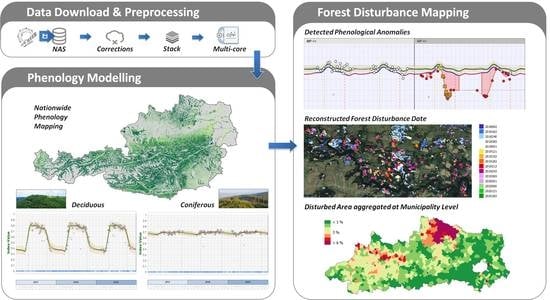
:Worldwide, forests provide natural resources and ecosystem services. However, forest ecosystems are threatened by increasing forest disturbance dynamics, caused by direct human activities or by altering environmental conditions. It is decisive to reconstruct and trace the intra- to transannual dynamics of forest ecosystems. National to local forest authorities and other stakeholders request detailed area-wide maps that delineate forest disturbance dynamics at various spatial scales. We developed a time series analysis (TSA) framework that comprises data download, data management, image preprocessing and an advanced but flexible TSA. We use dense Sentinel-2 time series and a dynamic Savitzky–Golay-filtering approach to model robust but sensitive phenology courses. Deviations from the phenology models are used to derive detailed spatiotemporal information on forest disturbances. In a first case study, we apply the TSA to map forest disturbances directly or indirectly linked to recurring bark beetle infestation in Northern Austria. In addition to spatially detailed maps, zonal statistics on different spatial scales provide aggregated information on the extent of forest disturbances between 2018 and 2019. The outcomes are (a) area-wide consistent data of individual phenology models and deduced phenology metrics for Austrian forests and (b) operational forest disturbance maps, useful to investigate and monitor forest disturbances to facilitate sustainable forest management.
1. Introduction
Worldwide forests are increasingly affected by changes and dynamics of various origin and at different scales [1,2,3]. Shifting patterns in timber demands [4,5] or in silvicultural perceptions [6] can constitute “sustainable” forest management, but can also trigger a change in timber harvest practises, including illegal logging and vast deforestation processes. Further, climate change effects on forest ecosystems accelerate forest mortality worldwide [7]. Forest biomes are the main terrestrial carbon stock [8]. Without doubt there is an urgent need to safeguard forested areas worldwide and trace dynamics of altering site conditions caused by climate change [7,9]. At the same time, forest product supply must be ensured, despite an increased multiuse demand concerning forest ecosystem functions [10]. Therefore, the monitoring of unobtrusive and small scale land cover changes such as those caused by natural events (e.g., pest infestation, higher mortality due to altering site conditions) or forest management practices (e.g., thinning or selective timber extraction) becomes more and more crucial [8,11]. Recent studies underlined the importance of a vital forest at stand or even single-tree level [12]. Forest disturbances can decrease the capability of forest ecosystems to protect against natural hazards, which is a major regulating function, especially of mountainous forests [13]. From a global perspective, it will not be sufficient to avoid deforestation to meet global climate change mitigation goals. Small-scale forest management has to be guided by the principles of sustainability too, because forest management has an unexpectedly large impact on standing biomass and related carbon sequestration [14]. On the one hand, the sustainable extraction of various forest products guarantees a young age structure, which can increase carbon sequestration rates up to 25% [15]. On the other hand, in mountainous terrain, unmanaged forests show a higher capacity of climate and erosion self-regulation compared to managed forests. Therefore, natural forests are more resilient to altering environmental conditions and will provide valuable regulating ecosystem services in the future [16]. The monitoring of such small-scale forest management practices will be crucial to guarantee sustainable forestry, not only in Austria.
Earth observation (EO) data has proved to be a comprehensive source to continuously assess the state of forests and to detect disturbances globally. Today image processing and analysis tools can map these changes and are increasingly capable of tracing slight phenology anomalies on different temporal scales, informing about intra-, inter- and transannual dynamics [7,9].
During the last few decades, EO programmes, such as Landsat [17] or MODIS [18] deliver data, which have enabled the implementation of large scale monitoring systems (e.g., Global Forest Watch [2]), as data provision is continuous and data quality consistent.
However, a phenological time series analysis (TSA) of global satellite imagery must cope with a highly varying topography and seasonal vegetation effects, compared to studies explicitly focusing on selected world regions that are less challenging (e.g., tropical forest or other biomes closer to the equator).
Austria, as an example of a country with diverse landscapes, shows distinct seasonality with low to high sun levels. The illumination conditions strongly vary, especially in alpine regions, due to topographic shadow areas, which affect the remotely sensed signal reflected by the Earth’s surface. During winter, snow cover and diverse weather patterns, such as invasive fog that is omnipresent in alpine valleys, significantly reduce the number of useful observations.
Previous research shows different methodological approaches to cope with these challenges. Most of the mainly Landsat-based TSAs rely on an image composite analysis [13,19] or on some variant of a harmonic modelling approach [13,19,20,21,22,23,24]. Harmonic modelling approaches are robust but show some limitations regarding the quality of temporal information [25] and allow only little detail in reconstructing seasonal vegetation courses. This limits the ability to depict the occurrence and magnitude of changes, which is needed to scrutinise dynamics on a forest management level. The COPERNICUS programme, the European Union’s earth observation programme [26], with its satellite twin consisting of Sentinel-2A and Sentinel-2B (S2) [27], provides new opportunities for monitoring forest ecosystems. The multispectral S2 sensor shows a spatial, spectral, and temporal resolution at a level which so far is unique in non-commercial EO. The ground resolution is up to 10 m and the revisit time is less than five days. The use of S2 data that is free of charge is quite established in agricultural monitoring [28,29] and non-forest phenology modelling [30], whereas advanced S2-based TSAs focusing on forest ecosystems are so far rare [31].
The Austrian Research Centre for Forests (in German: Bundesforschungszentrum für Wald—BFW) is, as a central federal research institution, focusing on forest state and forest future (BFW 2020). The BFW’s Department of Forest Inventory, responsible for the national forest inventory (NFI) in Austria, gathers, prepares and analyses nationwide information about forest state and dynamics [32]. New earth observation data, such as the S2 imagery, are a good supplement for existing terrestrial inventory data. Nationwide auxiliary data from remote sensing can compensate for weaknesses of sample-based inventory assessments [33,34]. The compilation of facts and figures for stakeholders and decision makers is a main task of the Austrian NFI. National to local forest authorities and other stakeholders increasingly request information concerning hot topics as storm damages, changing forest site conditions (e.g., tree species specific drought stress) or spatial patterns of pest invasions (e.g., the spread of bark beetle infestations) [8,11]. For these reasons, the BFW established and maintains a local archive for nationwide S2 data and develops operational data processing schemes to optimally exploit this data pool [11].
This article describes a novel TSA approach based on Sentinel-2 data, using a dynamic Savitzky–Golay phenology modelling algorithm [35]. The overall aim of the presented study is to develop an operational forest-monitoring approach that locates forest disturbances and accurately determines the date of their occurrence. To achieve this goal, our objectives are (1) to develop a straightforward workflow for modelling phenology courses from dense Sentinel-2 data time series, (2) to examine the suitability of several vegetation indices to deduce forest phenology features (phenology metrics) and to detect deviations from the modelled phenology courses (forest disturbances), and (3) to produce forest phenology and disturbance maps that comprehensibly visualize the information contained in the Sentinel-2 imagery.
2. Material and Methods
2.1. Material
2.1.1. Sentinel-2 Data
The proposed TSA approach relies on multispectral Sentinel-2A and -2B data. The approach uses the four spectral bands with a spatial resolution of 10 m of the top-of-atmosphere product (TOA, Level-1C), i.e., the bands B02 (blue), B03 (green), B04 (red), and B08 (near infrared). In theory, bottom-of-atmosphere (BOA) data are expected to be more suitable for time series analysis than TOA data. However, in previous tests it was found that BOA data produced by Sen2Cor (version 2.5.5) [36] are too error prone for a fully operational approach without any visual image checking and selection. Spectrally distorted pixel observations caused by atmospheric effects are, therefore, removed by outlier detection and filtering techniques, as explained in Section 2.2.4. We only use Sen2Cor’s quality grid outputs to derive a granule-wide mask to exclude pixels not useable for the TSA (Section 2.2.2).
We identified all S2 granules that intersect the area of Austria. In total, twenty granules were selected. All L1C datasets available for this area are stored in a local image archive that is updated on a regular basis by searching for and downloading new data with an oData-query via the ESA API hub [37]. The image archive contains data from the year 2017 and is updated regularly. For this study, images from January 2017 to December 2019 were available. The approach processes at least 75 images per granule and year.
In the TSA process, we distinguish two periods: (a) the model period (MP), and (b) the detection period (DP). The model period comprises one or more complete years. It is used to compute the reference phenology course. The detection period is the period that is examined for deviations from the reference phenology course. In the study, the model period is set to the period from 1st January 2017 to 31st December 2018 and the detection period ranges from 1st January 2018 to 31st December 2019.
2.1.2. Forest Map
To confine the TSA to areas covered by forest, a national forest map, produced at the BFW according to the Austrian NFI forest definition [38] is used. The vector map was resampled to the 10 m pixel grid of Sentinel-2.
2.1.3. Reference Datasets
For validating the class “Disturbance” of the forest disturbance map, we use field observations (in situ dataset) provided by the forest section of the Federal Government of Lower Austria. The data were collected during on-site inspections according to forest protection regulations between January 2018 and December 2019. The points are located in the north-western part of Lower Austria (Figure 1). The point attributes are the date of creation (in situ date), the number of affected trees and the disturbance type. The most frequent disturbance type is bark beetle infestation, followed by wind throw, wind breakage, snow breakage, and fungal attack. In the validation procedure, described in Section 2.5, all sites with at least three affected trees were considered, resulting in 1500 observations that could be used in the study.
For assessing the accuracy of the map class “No Disturbance”, we created a random sample dataset with 271 points for this stratum (Figure 1, red points) within the same area, where in situ data are also available. The number of sample points was chosen according to the recommendations provided by Olofsson et al. 2014 [39] with a target standard error for overall accuracy of 0.01. Each point was checked based on visual image interpretation, as described in Section 2.5.
2.2. Preprocessing
Images with a cloud cover of less than 80%, according to the L1C metadata file, are preprocessed. The preprocessing is divided into two parts: first, steps that are applied image by image (Section 2.2.1, Section 2.2.2 and Section 2.2.3), and second, steps that are applied to sets of images combined to multitemporal image stacks (Section 2.2.4 and Section 2.2.5).
2.2.1. Spectral Indices Computation
Because band ratios are less affected by atmospheric and topographic effects than single band values [40] we chose three spectral indices, suggested for vegetation analysis in literature, i.e., the Normalised Difference Vegetation Index (NDVI), the Green Normalised Difference Vegetation Index (GNDVI), and the Red-Green Vegetation Index (RGVI). In addition, we use the near infrared band, scaled by a factor of 5500 to get values between 0 and 1. Table 1 gives an overview of the spectral indices used in this study.
2.2.2. Cloud, Shadow, and Non-Forest Masking
We create masks to exclude pixels affected by clouds and shadows. The masks rely on several quality assessment outputs of ESA’s stand-alone atmospheric correction algorithm Sen2Cor (version 2.5.5) [36] that converts Level-1C (TOA) to Level-2A (BOA) data. We use a combination of a near-infrared threshold (B08L2A > 900), a cloud probability threshold (CLDL2A = 0) and a value selection of the land cover classification product (4 ≤ SCLL2A ≤ 5). Alternatively, cloud and shadow masks from other sources could be easily integrated into our workflow. Contaminated pixels that are not identified in this step are eliminated later by the outlier detection and filtering procedure (Section 2.2.4 and Section 2.2.5).
To exclude areas not covered by forest, we use the prepared NFI forest mask (Section 2.1.2).
2.2.3. Multitemporal Layer Stacking
After the granule-wide preprocessing steps, all images are combined to multitemporal layer stacks resulting in one layer stack per spectral index with a layer for each acquisition date. Missing values, e.g. due to clouds or shadows, are supplemented by no-data values. The next preprocessing steps are applied per pixel on time series vectors.
2.2.4. Outlier Filtering
The raw time series vectors are checked for unnatural discontinuities, i.e., an abrupt decrease followed immediately by a significant increase in the spectral signal. In forests, regreening processes (successive recovery) after disturbances occur rather slowly as compared to agricultural land, for example. Thus, such patterns are classified as outliers. They are excluded from the time series vector and are replaced by no-data values. The applied outlier criteria were empirically determined and are illustrated in Figure 2. A data point is classified as an outlier if the first two general criteria (Figure 2, criteria 1 and 2) and one of the remaining criteria (Figure 2, criteria 3a or 3b) are fulfilled. For outlier filtering, one previous and one subsequent data point are needed. Therefore, it cannot be applied to the first and the last data points of the time series.
2.2.5. Interpolation and Smoothing
After outlier filtering, data gaps are populated by linear interpolation to receive a continuous time series vector containing a value for each day of the year. Then a Savitzky–Golay Filter (SGF) [35] is applied to smooth the time series vector. The SGF is a moving window filtering method calculating polynomial functions that do not smooth the data excessively. We use a dynamic SGF-window width, because a fixed window width can lead to insufficient or nonmeaningful smoothing if the data are noisy [44]. The SGF is applied on the model period data and on the detection period data using different window settings, which were empirically determined as specified in Table 2.
For the model period, the window size is chosen in dependence on the index value range between the 85th percentile (P85) and the 15th percentile (P15), relative to the mean index value () of all data points in the model period, as specified in Table 2. In this way, the window size is automatically adapted to the vegetation type’s specific phenological variation. The dynamic window size results in a stronger smoothing effect for coniferous pixels (low phenological variation) than for deciduous pixels (high phenological variation).
As a result, we get for each pixel two smoothed time series curves per index with 365 values per year, i.e., one for the model period (MPTS) and one for the detection period (DPTS).
2.3. Phenology Modelling and Phenology Metrics
The smoothed multiyear course covering the whole model period is split into single-year snippets, resulting in a yearly vector for 2017, 2018, and 2019, respectively. Then a set of statistical parameters is computed over the three vectors for each day of the year. So, the information from all years within the model period is aggregated. Optionally, each year can be weighted individually, for example, to reduce the impact of previous years or of years with extreme weather conditions. In this study, all years were weighted equally. The set of parameters consists of the 10th, the 50th and the 90th percentile courses (PC10, PC50, PC90), as well as the mean of the two values PC10 and PC90. The set of percentile courses describes the inter-year index variability of all years within the model period. All four courses can serve as the reference phenology time series for the subsequent detection of anomalies (Section 2.4). In this study, we use the mean of PC10 and PC90 as the main phenology course (MPC) for the forest disturbance analyses.
Finally, a set of phenology metrics are extracted from the MPC. Phenology metrics are measures that allow for a straightforward, rather intuitive interpretation of phenological characteristics. In this study, we computed the phenological metrics "start of vegetation period" (SVP), "end of vegetation period" (EVP) as well as the maximum value of the MPC (MAXMPC) and the date when the MAXMPC is reached (MPCmax). For all dates, the day-of-year (DOY) notation is used. The SVP is the date, where the day-to-day gradient of the MPC is a maximum considering all values between DOY 90 (i.e., end of March) and DOY 182 (i.e., end of June). The EVP is the date where the day-to-day gradient of the MPC is a minimum, considering all values between DOY 245 (i.e., beginning of September) and DOY 340 (i.e., beginning of December). Other metrics, such as the growing season length or the number of phenology peaks, are not considered as they are beyond the scope of this study.
2.4. Anomaly Detection
Phenological anomalies are significant deviations of the spectral index from the “expected” course (base line). The base line (BL) is the MPC shifted in the Euclidean space to allow for more distinct deviation patterns in periods with a naturally high phenological variation (e.g., in spring and fall). The result is an “inward-buffered” reference course. Thereby, the detection of anomalies is robust in terms of slight shifts of the course along the time axis (e.g., a shifted start of the vegetation period). Such shifts can occur, for example, due to varying weather conditions from year to year.
For anomaly detection, the cumulative sum of the daily difference between the BL and the smoothed detection period curve (DPTS; Section 2.2.5) is computed for each pixel. The cumulative sum of daily index deviations serves as a proxy for the emergence and manifestation of anomalies [45,46,47]. Periods with an insufficient number of data points (usually in winter) are ignored in the calculation. The beginning and the end of the considered period are not set to fixed dates but are chosen according to the available data. For this, all observations in the MP are pooled as if they were collected within one year. Then the day-of-year (DOY) values are determined that correspond to the 2nd and to the 98th percentile. These dates serve as the beginning and the end of the period for calculating the cumulative sum of deviations. Optionally, the last m data points at the end of the time series can be omitted in the cumulative sum calculation, usually with 0 < m < 2 to avoid incorrect results induced by data points that could not be filtered and smoothed by subsequent observations. For ad hoc results, e.g., right after a storm event, however, m = 0 is recommended because otherwise the most recent deviations cannot be detected. In this study, m = 1 is used. The date of the last effective data point used for the TSA is called "last usable observation" (LUO).
For forest disturbance analysis, two pieces of information are important, i.e., the level of disturbance and the date of disturbance. Both pieces of information are deduced from our high-density times series.
The forest disturbance level (FDL) is measured by means of the cumulative sum of daily index deviations (Equation (1)) with FDL = 1 corresponding to a cumulative sum equal to 1 and so on.
The FDL is a kind of measure to identify pixels that are affected by a certain level of disturbance. The FDL refers to the severity and the duration of the disturbance. The higher the FDL, the higher the level of manifestation of the disturbance. In this study, the threshold for the FDL (TFDL) is set to a medium level of 7, meaning that all pixels with an FDL of 7 and higher are labelled as disturbance pixels. In addition to the information, whether or not a pixel is a disturbance pixel, the date when the specified FDL is reached is stored, called the Cumulative Deviation Date (CDD; Equation (2)).
Beyond that, for each disturbance pixel, the date is reconstructed in a backwards direction when the identified disturbance shows up in the data the first time during the backwards reconstruction, called the Forest Disturbance Date (FDD). The FDD is a "theoretical" date estimated from the BL and the actual (non-modelled) index course. It is the date, when both curves intersect for the last time, previous to the corresponding CDD.
All features (CDD, FDD, etc.) are exported as grids with a spatial resolution of 10 m. So, as a result, we get maps that report for each Sentinel-2 pixel if it shows anomalies according to the specified level of disturbance and, if true, an estimated date corresponding to the starting point of the abnormal spectral behaviour.
2.5. Validation
The TSA’s ability to detect disturbance events is assessed by checking the derived forest disturbance map at the positions of the in situ observations (Section 2.1.3). To account for spatial deviations between the Sentinel-2 data and the in situ data, the area within a radius of 20 m around each point is considered. The detection of the disturbance event is regarded as successful if there is at least one disturbance pixel within this area. Additionally, the minimum FDD of all disturbance pixels per point within the specified circle is computed. We chose the minimum FDD as a benchmark, because usually one aims at detecting forest disturbance events as early as possible, both in the field and by means of remote sensing.
Based on this dataset, the detection rate, i.e., the number of detected disturbance events divided by the total number of disturbance events in the in situ data, is computed. For the temporal evaluation, the date difference (in situ date minus FDD) is analysed.
To complete the validation, we manually check the forest disturbance map at randomly selected positions within the “No Disturbance” stratum (Section 2.1.3) based on visual interpretation of a series of Sentinel-2 images. For this inspection, cloud-reduced natural- and false-colour-composite mosaics of Sentinel-2 images from spring, summer, and fall of 2018 and 2019 are used. For each point, including a 3 by 3 pixel neighbourhood, it is visually checked if the spectral signature is stable (corresponding to the class “No Disturbance”) or changing (corresponding to the class “Disturbance”) over the deviation period. In the case of deciduous forest, mainly the summer images are considered to avoid misclassifications due to seasonal phenology changes.
2.6. Implementation
The entire workflow is implemented via the open source software "R" [48], benefitting from its comprehensive package libraries, primarily raster [49], rgdal [50], gdalUtils [51], rgeos [52], doParallel [53], foreach [54] and signal [55]. All processed data are saved on a local network-attached storage (NAS). The computation-intensive TSA approach highly relies on memory-optimised and parallelised computing: first during the parallelised batch-mode of Sen2Cor, second when copying the data from the NAS to the local environment and third when executing the per-pixel TSA itself. The implemented parallelisation allows for the full use of all CPU-power available.
3. Results
Following the structure of the method section, the results section presents the main findings concerning (1) the phenology modelling with Sentinel-2 time series applied to the entire forest area of Austria (Section 2.3), and (2) the multiyear forest disturbance mapping, focusing on damages by the bark beetle infestation in Northern Austria (Upper and Lower Austria) between 2018 and 2019 (Section 2.4).
3.1. Phenology Modelling with Sentinel-2 Time Series
The phenology modelling procedure analyses per-pixel time-series data, covering more than 40,000 km2 of forest area in Austria, which results in around 400 million unique models per spectral index. The models comprise Sentinel-2 data from the years 2017 to 2019. In Figure 3 and Figure 4 examples of phenology courses typical for deciduous and coniferous forest are plotted together with detailed additional information, such as phenology metrics, derived from the time-series data.
The white dots indicate valid data points. The grey dots are data points excluded by the outlier filtering procedure. The blue circles at the bottom of the plot show all available data points (from granules with more than 80% valid pixels), including observations that were eliminated, e.g., due to clouds or shadows. Each graph comprises the 10th percentile index course (thin red line), the 90th percentile index course (thin green line), and the resulting MPC (bold dark green line). The brownish ribbon represents the variability of the MPC. It is plotted just for illustration. The pixel plots show significant differences, depending on the forest type. Pixels representing deciduous forest (Figure 3) show generally more variation over the year than pixels representing coniferous forest (Figure 4).
The seasonal course patterns typical for deciduous and coniferous forest vary from index to index. In general, the average NDVI- and RGVI-values are higher, compared to the GNDVI and the BNIR, both for deciduous and coniferous forest. The seasonal course pattern of MPC is less distinct for GNDVI and RGVI than for NDVI and BNIR. The latter shows a notable peak in spring to early summer, highlighting the BNIR’s higher sensitivity to depict vegetation productivity. These temporal differences in the MPCs underline that each spectral index has special characteristics.
The deviations of the data points from the MPC (noise) vary from index to index. For pixels of coniferous forest, the RGVI noise is clearly the lowest compared to the other indices, whereas for pixels of deciduous forest, RGVI noise is the highest.
The vertical lines in blue indicate selected phenology metrics. The first one (solid line) denotes the date when MPC reaches its maximum (MPCMax). Deciduous forest pixels show basically higher maximum MPC values (MAXMPC) than coniferous forest pixels (Figure 3 and Figure 4).
Figure 5 shows the NDVI-based MAXMPC map for Austria, limited to forest. The values range from about 0.5 to 1.0. The highest values of 0.8 and higher are found in areas covered by deciduous forest, such as in the north-eastern part of Austria. NDVI values around 0.65 indicate spruce-dominated areas, as existing in alpine regions or in the northern parts of Austria. Lowland pine stands and high-alpine dwarf pines, for example, show values below 0.55.
The start date of the vegetation period (SVP) and the end date (EVP) are denoted by dashed lines. SVP and EVP slightly differ depending on the used index and can significantly vary between different forest types and locations. Figure 6 shows the SVP for Vorarlberg, the most western region of Austria, derived from the GNDVI model of the years 2017 to 2019. Early SVPs (about mid of April) mainly occur in areas of low to mid altitudes dominated by broadleaved tree species, as found in the western and northern part of Vorarlberg. Late SVPs are mainly found in areas covered by coniferous forest, such as in the alpine region in the south of Vorarlberg. At a closer look, one can also see heterogeneous spatial patterns and distinct differences in the SVP that can be explained by differences in the elevation and the tree species composition (Figure 6, right).
3.2. Forest Disturbance Mapping in Northern Austria
The presented forest disturbance mapping results are based on the RGVI that proved to be the best index for negative deviation detection as it shows little noise and robust courses. This is especially true for coniferous forest (Figure 4). For the presentation of the forest disturbance results, we chose the northern region of Austria, which is currently a hotspot in terms of bark beetle infestation.
First, we exemplify the basic results of the per-pixel anomaly-detection procedure using four pixels (Figure 7, P1 to P4) selected from the study area that represent typical events when dealing with forest anomaly detection. Note that the last data point of each pixel time series is excluded from the TSA (Section 2.4). Excluded data points are highlighted by a grey dashed ellipse.
Example P1 (Figure 7, first row): In 2018, the first year of the detection period (DP), the index course shows the same stable and inconspicuous trend as in 2017. In 2019, however, we observe gradually lower values. In early June 2019, a strong disturbance occurs, finally reaching the deviation level FDL-7 on 30th June (CDD, orange marker). The red area below the baseline (BL, blue line) corresponds to the cumulative deviation of the time series. The date of origin of the disturbance (FDD-7, yellow marker) is estimated to be 9th February 2019. The data points after the CDD-7 label, all of them lying significantly below the baseline, confirm the detected disturbance.
Example P2 (Figure 7, second row): The pixel shows a disturbance occurring between 13th July 2018 and 4th August 2018. The medium damage level (FDL-7) manifests in early September (CDD-7 = 11th September) and the related FDD-7 is July 22nd 2018. In this example, the main deviation happens in the period, when MP and DP overlap. The index course and the resulting deviation area (red area) of 2019 clearly confirm the disturbance detected in 2018. Note that the winter period is excluded when computing the cumulative deviation sum (no red area between mid of October and beginning of April), because the number of data points is not sufficient (Section 2.4).
Example P3 (Figure 7, third row): The time series of this pixel follows the modelled course and no change is detected. Only the last data point possibly indicates a major deviation, but this data point was excluded in the truncation process described in Section 2.4. Further observations are required to confirm or discard this assumption.
Example P4 (Figure 7, fourth row): This pixel does not show any anomalies until November 2018, but after the excluded winter period, a severe change becomes evident, reaching FDL-7 on 20th April 2019. The corresponding FDD-7 is traced back to 5th December 2018. This example represents common winter dynamics, such as forest management activities (e.g., clear-cutting, selective timber extraction or thinning) or natural disturbances (e.g., snow and avalanche damages).
Figure 8 shows the FDD-7 map for a subset of the study area, including the pixels P1 to P4 presented in Figure 7. The selected area is heavily affected by recurring bark beetle infestations [56]. In the background, Sentinel-2 RGB-composites (10 m, Level L2A), acquired in Sep. 2017 (Figure 8a,b), Sep. 2018 (Figure 8c,d) and Sep. 2019 (Figure 8e,f) are shown.
Figure 8b highlights the pixels where FDD-7 is in 2018 (dark-blue–blue–white). Figure 8d additionally highlights the pixels where FDD-7 is in 2019 (white–yellow–orange–red–pink). The FDD map shows rectangular to round patches of change, most of them with an FDD minimum (earliest date) close to the centre of the patch surrounded by continuously increasing FDD values, which is a characteristic pattern of spreading in the context of bark beetle infestation. Areas with a late FDD (near the end of the year 2019) are usually found in close proximity to areas with an earlier change (lower FDD).
The FDD maps can be spatially aggregated at any level. Figure 9 illustrates three FDD-mapping products, computed for the whole study area: (a) the original FDD-map—simplified to the categories “Disturbance” and “No Disturbance”—with a spatial resolution of 10 m, (b) the percentage of forest area affected by forest disturbance for hexagons of 100 hectares, and (c) the percentage of forest area affected by forest disturbance at municipality level.
It was found that forests at higher altitudes show generally less disturbance than forests in lowland areas. In total, the disturbed forest area is 23,400 hectares, i.e., on average 2.8% of the forest area in the study area. The forest disturbance is not evenly distributed over the whole study area but concentrates on a few regions (Figure 9). Approximately, one quarter of all municipalities show an affected forest area of more than 4%, comprising primarily municipalities of the regions “Lower Mühlviertel” and “Innviertel”, of the central region of Upper Austria and foremost of the region “Northern Waldviertel”.
3.3. Validation
The validation results of the in situ dataset show that, in 1251 out of 1500 in situ cases, the TSA identified a disturbance. In 249 in situ cases, the Forest Disturbance Date grid (FDD-7) does not show a disturbance. So, the TSA identified 83.4% of the disturbances recorded by field data (Table 3).
The validation results of the random sample dataset show that 258 out of 271 random points (95.2%) could be verified, by visual interpretation, to be not disturbed. In 13 cases, we observe phenological deviations, which are not detected by the TSA.
The histograms in Figure 10, Figure 11 and Figure 12 show the temporal difference (in days) between the in situ date and the FDD. The bin width is 30 days. The black line in the centre denotes a difference of zero, which means that the FDD is equal to the recorded in situ date. Counts to the left of the line (negative date difference) indicate disturbance events, where the theoretical FDD of the TSA lies after the in situ date. Counts to the right of the line (positive date difference) correspond to cases, where the TSA detects disturbances earlier compared to the field observations.
The first histogram (Figure 10) comprises all 1251 cases with an FDD from January to December. There are 358 counts on the left and 893 counts on the right (29% and 71%). The column of the first bin on the right (0 to +30 days) is the highest of all and includes 233 cases (19%).
The second histogram (Figure 11) comprises a subset of Figure 10 including only counts outside the vegetation period with FDDs from October to April. In total, there are 657 cases with 218 counts (33%) on the left and 439 counts on the right (67%). The maximum on the right side indicates that the TSA detects disturbances with FDDs outside the vegetation period about 130 days earlier compared to the corresponding in situ date.
The third histogram (Figure 12) comprises a subset of Figure 10, including just counts within the vegetation period with FDDs from May to September. In total, there are 594 counts with 140 counts on the left (24%) and 454 counts on the right (76%). The graph indicates that, for disturbances with FDDs within the vegetation period, the FDD strongly correlates with the in situ date. The column of the first bin on the right side (0 to +30 days) is the highest of all and includes 211 cases (36%). About 51% of the cases have an FDD that deviates less than ±30 days from the in situ date, and about 69% of the cases have an FDD that deviates less than ±60 days from the in situ date.
4. Discussion
4.1. Phenology Modelling with Sentinel-2 Time Series
4.1.1. Take-Home Messages
The approach described in this article uses a new and advanced workflow to compile, preprocess and analyse dense Sentinel-2 (S2) time series. The presented TSA approach uses all S2 granules with less than 80% cloud cover available for a chosen period. The approach significantly benefits from the improved data availability due to the launch of the Sentinel-2B satellite in spring 2018. Thereby, very dense time series can be compiled, allowing for the application of advanced fitting methods. With such methods, intraseasonal variations can be preserved [25] and phenology developments can be traced with a high level of detail.
Recent studies stressed the capabilities of an updating S2 time series that predicts forest phenology using a recursive Kalman filter [31]. Unlike these studies, we use a Savitzky–Golay filtering (SGF) approach, as former studies showed the advantages of SGF to smooth out signal noise but retain temporal details. This holds true for dense time series analyses, such as S2-imagery time series [57].
The presented TSA is based on a dynamic SGF approach [35]. We use a dynamic window width, because a fixed window width can lead to insufficient or non-meaningful smoothing if the data is noisy [44]. So far, SGF has primarily been used with remote sensing data of medium resolution (e.g., MODIS with 250 m) and a fixed and rather wide window that results in a high degree of generalisation [57,58]. Most TSA studies based on Sentinel-2 or Landsat data, apply harmonic regressions (ordinary least square models) on the generated time series to characterise the seasonality of the vegetation canopy [24,25,47,59]. The periodic character of harmonic regression models, the fast computing time and the robust results are clear advantages of harmonic regressions and in the case of lower frequencies of data, they may be the only option for achieving robustness [25]. However, they become impractically complex when describing phenology courses with a more segmented type of the seasonal phenology dynamics, as it is in the case of forests in the mid-latitudes. Forest vegetation in the mid-latitudes goes through an inactive winter period, a sharp greening period in spring, followed by a slightly lower stable state in summer, and a constant defoliation process in fall, which is substantially different to vegetation in tropical regions with a more smoothed gradual phenology course.
The approach described in this article is based on TOA data, referred to as Level 1C (L1C). According to our experience, BOA data, referred to as Level 2A (L2A), produced with the Sen2Cor algorithm, provided by ESA, have considerable radiometric deficiencies, such as effects of overcorrection. Due to these problems, quite a few images cannot be used in the TSA, although the original images (L1C) are of good quality. Thus, we clearly get denser time series with L1C data than with L2A data. On the downside, L1C data are affected by mainly atmospherically induced noise, which is, however, successfully reduced by efficient outlier filtering and smoothing.
The innovative multiyear percentile modelling approach traces high courses (90th percentile) and low courses (10th percentile) of single year time series, whereas the mean of both provides robust multiyear courses (MPC). The MPC levels out extreme years, which further reduces distortions caused by possible outliers.
As a byproduct, the phenology modelling procedure delivers meaningful phenology metrics (e.g., Figure 6). Phenology metrics, such as the start and end of vegetation period [60,61,62], can be deduced for deciduous forest pixels quite easily, due to the typical seasonal characteristics. For coniferous forest pixels, it is more challenging. Here the dynamic SGF window width proves to be an appropriate mean to deduce reasonable metrics across various forest types and forest growing regions in Austria. Phenology metrics and the reliable MPCs can be used for various downstream analyses, such as for forest type classification [63] or habitat modelling.
4.1.2. Limitations
The accuracy of the TSA results is dependent on the data availability, which varies significantly from region to region. Primarily, the number of available observations per year is determined by the revisit time. This is at least 5 days and is halved in areas where the swaths overlap. In addition, local weather conditions, such as clouds and cloud shadows, and factors concerned with topography, such as topographic shadows and snow coverage, determine the actual data point density. In some regions of Austria, we can compile up to about 40 valid data points per year for the TSA (Figure 13). In swath overlapping areas, we can utilize 30 to 35 data points on average. In areas where the swaths do not overlap, the TSA can make use of about 15 to 20 data points on average. The single pixel courses, shown in Figure 3 and Figure 4, lie in areas of overlapping swaths with significantly more observations than the single pixel courses, shown in Figure 7, that lie in areas without overlapping swaths.
4.1.3. Implications
The TSA provides large area phenological information about the Earth’s surface covered by vegetation. Although the approach was developed in the context of forestry, with a focus on forest applications, it also shows a high potential for interesting applications in other fields, such as conservation ecology, social ecology, and agriculture. The reconstructed phenology models provide an outstanding database not only for habitat modelling or wall-to-wall forest-type mapping, but also for models used for biomass and carbon stock estimation. Multitemporal and, in particular, phenological information, also play an increasing role in the analyses of nonforest environments. Crop type classification and monitoring [28,64,65,66,67], the reconstruction of the harvesting time of crops, cycle durations or the delineation of multiannual crops can benefit from the TSA and its outputs. For grassland management, the systematic capturing of cutting times would be highly relevant (e.g., for funding provided by the European Union) [68,69].
4.1.4. Recommendations
The described TSA is constantly adjusted, improved and extended. This comprises the used input data, parameter tuning, new analysis tools and downstream applications.
So far, the TSA relies on some Sen2Cor products, but the used indices are based on L1C values (no atmospheric correction), due to Sen2Cor-failures. In the long run, we aim to use atmospherically corrected input data. Other preprocessing procedures (e.g., ATCOR [70]), as alternatives to the Sen2Cor algorithm, still need to be tested. Consistent surface reflectance data would clearly be beneficial to further reduce signal noise effects.
The general data availability, the annual distribution of valid observations and the seasonal data variability constitute unique phenology courses on a per-pixel level. These unique time series require dynamic parameters (e.g., SGF-polynomial order, tree species dependent smoothing factor, data gap detection) for individual modelling in terms of outlier filtering, interpolation, smoothing, and multiyear data fusing. We plan to further optimise existing parameters and introduce new dynamic parameters.
In the next years, the TSA can be used to study long-term trends caused by climate change. Multiyear fusions of more than about five years will allow for investigating spatiotemporal shifts in forest phenology patterns. We are confident that the TSA will meet future demands of tracing altering site-specific forest phenology, including slightly changing tree species compositions or shifting growing periods.
4.2. Forest Disturbance Mapping in Northern Austria
4.2.1. Take-Home Messages
In the last decade, North America and Europe experienced massive bark beetle outbreaks with serious impacts on the landscape, forest industry, and ecosystem services. The extent and intensity of many recent outbreaks are widely believed to be unprecedented [71]. Therefore, there is an urgent need for operational tools to assess the affected area fast and reliably over large areas [11]. The presented TSA approach proves to be a proper forest monitoring tool for large-scale analysis as demonstrated in a test region located in Upper and Lower Austria. We found severe phenology anomalies, especially in the northern parts of this region, which corresponds well to recent reports about bark beetle calamities in Austria [56].
The main benefit of the described forest disturbance mapping approach is its ability to determine and map the date when an anomaly occurs with a high level of detail. The TSA can reconstruct a theoretical intra-annual forest disturbance date (FDD), expressed in the day-of-year format and with a spatial resolution of 10 m.
The FDD validation (Section 3.3) shows that 83.4% of the recorded field observations were successfully detected by the TSA. The results confirm that the anomaly detection procedure performs well. The error of omission of about 16% can be explained, to some degree, by the way the in situ data were collected, as discussed in Section 4.2.2. Furthermore, the validation results for the class “No Disturbance” with an agreement of 95.2% confirm that the TSA provides results with high accuracy.
Overall, we can reconstruct and map the forest disturbance date with a high level of detail on the time axis, as shown in Figure 8. Such maps compactly visualize the comprehensive spatiotemporal information contained in dense Sentinel-2 time series and can make a substantial contribution to the assessment and monitoring of forest disturbances.
The FDD maps (Figure 8) show patches of disturbance that are growing in a ring-like manner. These spatiotemporal disturbance patterns are typical for the spreading of bark beetle infestations [72]. They result from a temporal sequence of timber harvesting to counteract further bark beetle spreading. The detected patterns also indicate that the FDD maps are plausible. Otherwise, they would show a rather random distribution of disturbance patches.
The anomaly detection procedure is very flexible in terms of the disturbance level to be detected. This is realized by using the cumulative sum of deviation as a measure for disturbance. The sensitivity level threshold for the FDL (TFDL) can be chosen, corresponding to different degrees of forest disturbance. The optimal level of sensitivity depends on the overall goal. FDL thresholds from 5 (very sensitive) to 10 (highly reliable) were found to be most reasonable. We recommend stepwise processing with a range of FDL thresholds and finally to choose the FDL threshold that is most appropriate. In this article, results for a TFDL of 7 (CDD-7/FDD-7) are shown, corresponding to a medium detection sensitivity (i.e., minor anomalies are not considered).
The applied anomaly detection approach, based on dynamic SGF modelling, shows a high temporal sensitivity. In the vegetation period (May–September) we can detect more than half of the disturbances within at least ± 30 days using the in situ date as a reference. Future studies need to investigate the strengths and weaknesses of the temporal TSA outputs, compared to similar information derived by approaches based on generalised harmonic model fitting and trajectory segmentation, which are widely established to detect temporal breakpoints in a time period of interest [45,46].
The TSA approach is expected to be suitable for different use cases, ranging from rapid disturbance mapping (e.g., after storm events) at local or regional scale to operational nation-wide disturbance mapping. Depending on the use case, different parameter configurations can be chosen.
For anomaly detection, we chose the vegetation index, RGVI. It was found to be useful particularly for detecting anomalies in coniferous forests which generally show index courses with little seasonal variation. Among all considered indices, the RGVI shows the lowest seasonal variation, which is preferable when it comes to anomaly detection. In this study, which concentrates on forest disturbances in coniferous forests, the RGVI index proved to be very efficient to detect distinct, as well as marginal vegetation, anomalies in the time series and can be recommended for studies on bark beetle infestation.
In general, some indices are more suitable to detect forest disturbances, others are more useful to derive phenology metrics (Figure 3 and Figure 4). The GNDVI, for example, is probably a good candidate for analysing shifted spring greening due to seasonal drought stress. Here further research is needed.
4.2.2. Ground Truthing
A quantitative validation of TSA outcomes is generally difficult, as is the case for many monitoring applications based on remote sensing data [73,74]. Ground truth data that comprise temporal information on land cover changes are rare. Besides, it is generally difficult to obtain data on disturbances that are consistent over large areas, because how it is collected often varies with the responsible institution or person.
Being aware of all these challenges, the in situ validation dataset used in this study cannot be valued highly enough. Nevertheless, there are some limitations. First of all, reference data for the category “No Disturbance” is missing. Therefore, it cannot be used to estimate the rate of true negatives and false positives. In this study, this shortcoming is compensated by an extra reference dataset obtained by visual image interpretation. In future, in situ data for both classes, “Disturbance” and “No Disturbance”, are desirable.
In addition, the in situ date, i.e., the date when the site was visited, does not necessarily correspond to the date when the disturbance event happened and became evident in the spectral signature the first time. This fact limits the possibilities of temporal evaluation.
The in situ data were not collected with the purpose of validating remote sensing-based products but with the purpose of documentation. Therefore, the data points are often placed close to but not within the affected groups of trees or forest stands. This fact may lead to an underestimation of the derived detection rate. Thus, the accuracy figures reported in this study are assumed to be rather conservative.
4.2.3. Limitations
The quality of the anomaly detection results is heavily dependent on the data availability, which can vary from pixel to pixel, as described in Section 4.1.2. The validation (Section 3.3) was done in an area where the Sentinel-2 swaths do not overlap with about 15 to 20 observations per year. Therefore, our results suggest that the number of data points usually available is sufficient to reliably detect forest disturbances. Only in areas where the data availability is additionally reduced by clouds, shadows or snow do we expect limitations. Therefore, in alpine regions a temporally precise reconstruction of forest disturbance dates remains challenging.
The exclusion of one or more data points at the end of the time series guarantees that only anomalies are considered that are affirmed by following data points. In this way, the risk of mapping false positives can be reduced. However, for “near-real-time” applications (e.g., the mapping of storm damages within a narrow time frame) the most recent data points are indispensable and consequently the risk of false positives has to be accepted.
The FDD-validation histogram of FDDs outside the vegetation period shows a skew distribution (Figure 11). The maximum of counts shifted from zero to the right, which can be explained by two reasons. First, compared to the vegetation period, there is a tendency that foresters note possible bark beetle infestations with a time lag. Second, the current reconstruction approach of the FDD shows some constraints in winter. If the disturbance lies in the winter period with insufficient data points and, therefore, the deviation calculation is deactivated, the TSA shows the tendency to result in too-early FDDs.
In this study, the modelling period and the deviation period partly overlap. This should be avoided in the future and was only accepted here because, when the study was carried out, the Sentinel-2 data archive comprised only three complete years (2017, 2018, and 2019) of consistent data. Alternatively, a baseline derived from Landsat data could be used. Phenology modelling could benefit from the much longer time-series compared to Sentinel-2. This is especially true if minor anomalies are to be detected. However, the integration of Landsat data also comes with some negative effects, primarily the lower spatial resolution of Landsat compared to Sentinel-2 as well as the differences in the spectral characteristics between Sentinel-2 and Landsat.
4.2.4. Implications
The spatiotemporal information provided by the FDD maps is highly relevant for the pest control management typically conducted by local forest authorities. At the same time, the approach can also be applied on larger scales, such as at the national level and providing information for stakeholders and policymakers. The presented TSA approach is not designed for the early detection of bark-beetle-attack—also referred to as “green-attack”,—detection, which is currently a hot topic both in forest management and research. However, the FDD maps are a unique data source for entomological studies investigating the spreading behaviour of bark beetles. Beyond the assessment of natural disturbances, anomalies also caused by activities, such as illegal logging, are assumed to be detectable.
Further, the anomaly detection results deliver reliable information for a systematic large-scale assessment of forest disturbances with a spatial resolution of 10 m. For large parts of Northern Austria, the aggregated results (Section 3.2) reveal that the disturbed forest area is much too large for being consistent with sustainable forest management, according to the commonly used forest management model called “Normalwaldmodell” in German. The “Normalwaldmodell”, according to Hundeshagen [75], is used to determine the annual allowable cut in the case where forest management is focused on even-aged, monospecific stands. The model is characterized by a specific production cycle (rotation period) and a uniform area distribution of the corresponding age-classes.
If we assume a relatively low average rotation period of 80 years for spruce stands [76], an annual harvest rate (including unscheduled timber extractions) of up to 1.3% is sustainable. Thus, from a forest management perspective, more than 4% (i.e., 2% per year) of harvested forest area in the period from 2018 to 2019, as it was found in some regions within the study area, clearly indicate unsustainable developments. At least a quarter of the investigated municipalities—for whatever reason—show such dynamics. This underlines that zonal statistics covering different scales, and different damage levels are of high relevance for the forestry sector. Zonal statistics provide aggregated overviews and comprehensively inform policy makers and stakeholders about the extent of forest disturbances.
4.2.5. Recommendations
The presented TSA is able to detect anomalies, but so far it cannot distinguish between different causes of anomaly, such as bark beetle infestations, storm events or timber harvesting activities. However, this information is very important, for example, to specifically assess the amount of damage caused by bark beetle infestation [11]. Previous studies have already tried to discriminate different categories of change by directly using various disturbance metrics or by using those metrics as input data for machine learning algorithms (e.g., Random Forest) [20,77,78,79,80]. First tests based on our data suggest that there are specific patterns both in the single pixel courses as well as in the FDD maps that could help to categorize disturbances by the cause of disturbance. The validation data source used in this study possibly provides appropriate training data to distinguish different forest disturbances. This issue will be addressed in follow-up studies.
So far, we have concentrated on coniferous forests as in Austria this forest type is most affected by natural disturbance processes. Thus, there is a need to also fine tune the TSA for deciduous forests.
5. Conclusions and Perspectives
In this study, we present the first nationwide operational forest phenology modelling and forest monitoring system optimised for 10 m Sentinel-2 time series data and based on a Savitzky–Golay modelling approach. The method was successfully tested in Austria and is expected to also be applicable in many other regions all over the world.
Overall, the study shows that, even with TOA data, instead of BOA data, the robust forest phenology modelling is feasible. Even so, further tests with atmospherically corrected data (e.g., from ATCOR [70] or an improved Sen2Cor version) are planned. The workflow is very flexible so that the TOA data can be replaced by BOA data without any effort. Besides, the TSA is extendable to additional input data. In a next step, the Sentinel-2 20 m bands will be included in the TSA.
The main benefit of the described approach, compared to Sentinel-2 approaches that exist so far, is its capability to derive meaningful phenology courses without eliminating intra-annual characteristics at the same time. Our TSA is more than a fixed sequence of single snapshots. It is capable of balancing between temporal sensitivity and certainty, as different applications need differently adjusted TSA-settings. Besides the basic index choice, we can define various parameters as BL-offset from MPC, smoothing degree, and many more.
Important outputs of the TSA are day-of-year spectral quantities (e.g., MAXMPC for the NDVI) and seasonal metrics (e.g., start of vegetation period). These output features offer the opportunity to derive area-wide consistent wall-to-wall products. They are relevant to NFIs for many purposes.
Recent efforts of the Austrian NFI have aimed for operational implementation to use phenology modelling metrics to derive reliable nationwide forest type maps. Forest type classifications [81] will definitely benefit from such consistent input data. The resulting forest type maps can, for example, further improve the biomass estimations of NFIs [34].
The main added value of the presented TSA is the provision of novel temporal information about forest phenology anomalies. The TSA does not only map phenology anomalies with a high spatial resolution but also assigns a time stamp to each disturbed pixel with a high temporal resolution, indicating the estimated date when the anomaly is recognizable in the dataset the first time. The high sensitivity of the TSA’s outcomes serves the forestry and forest ecosystem sciences’ aim to monitor forests. Finally, the TSA also opens new fields for various applications on a forest-management level. Here the described nationwide wall to wall application, which focuses on bark beetle damages, demonstrates that the TSA is a useful monitoring system to scrutinise spatiotemporal patterns of forest disturbance. The results of this study show that it is possible to map the spreading of bark beetle infestations and other disturbances with a high accuracy.
The upcoming decades demand long-term analytic tools that focus on the incremental impact of climate change effects on forest ecosystems. Therefore, subsequent efforts should extend the TSA in such a way that also transannual anomalies can be captured.
Author Contributions
M.L. prepared the imagery data, developed and implemented the time-series algorithm and performed downstream analyses from the time series outputs. T.K. was a major contributor in interpreting the results and in writing the manuscript. Both authors have read and agreed to the published version of the manuscript.
Funding
This research received no external funding.
Acknowledgments
Thanks to the forest section of the Federal Government of Lower Austria for providing the in situ data, to Ambros Berger for revising the manuscript and three anonymous reviewers whose comments helped to improve this paper.
Conflicts of Interest
The authors declare no conflict of interest.
References
- Kindermann, G.; McCallum, I.; Fritz, S.; Obersteiner, M. A Global Forest Growing Stock, Biomass and Carbon Map Based on FAO Statistics. Silva Fenn. 2008, 42, 387–396. [Google Scholar] [CrossRef] [Green Version]
- Hansen, M.C.; Potapov, P.V.; Moore, R.; Hancher, M.; Turubanova, S.A.; Tyukavina, A.; Thau, D.; Stehman, S.V.; Goetz, S.J.; Loveland, T.R.; et al. High-Resolution Global Maps of 21st-Century Forest Cover Change. Science 2013, 342, 850–853. [Google Scholar] [CrossRef] [PubMed] [Green Version]
- Mackey, B.; DellaSala, D.A.; Kormos, C.; Lindenmayer, D.; Kumpel, N.; Zimmerman, B.; Hugh, S.; Young, V.; Foley, S.; Arsenis, K.; et al. Policy Options for the World’s Primary Forests in Multilateral Environmental Agreements. Conserv. Lett. 2015, 8, 139–147. [Google Scholar] [CrossRef] [Green Version]
- FAO Forests, the Global Carbon Cycle and Climate Change. Available online: http://www.fao.org/3/XII/MS14-E.htm (accessed on 26 April 2020).
- Henders, S.; Persson, U.M.; Kastner, T. Trading Forests: Land-Use Change and Carbon Emissions Embodied in Production and Exports of Forest-Risk Commodities. Environ. Res. Lett. 2015, 10, 125012. [Google Scholar] [CrossRef]
- O’Hara, K.L. What Is Close-to-Nature Silviculture in a Changing World? Forestry 2016, 89, 1–6. [Google Scholar] [CrossRef]
- McDowell, N.G.; Coops, N.C.; Beck, P.S.A.; Chambers, J.Q.; Gangodagamage, C.; Hicke, J.A.; Huang, C.; Kennedy, R.; Krofcheck, D.J.; Litvak, M.; et al. Global Satellite Monitoring of Climate-Induced Vegetation Disturbances. Trends Plant Sci. 2015, 20, 114–123. [Google Scholar] [CrossRef] [Green Version]
- Birdsey, R.; Pan, Y. Trends in Management of the World’s Forests and Impacts on Carbon Stocks. For. Ecol. Manag. 2015, 355, 83–90. [Google Scholar] [CrossRef]
- Goetz, S.; Dubayah, R. Advances in Remote Sensing Technology and Implications for Measuring and Monitoring Forest Carbon Stocks and Change. Carbon Manag. 2011, 2, 231–244. [Google Scholar] [CrossRef]
- Matthews, E.; Payne, R.; Rohweder, M.; Murray, S. Pilot Analysis of Global Ecosystems: Forest Ecosystems; World Resources Institute: Washington, DC, USA, 2000. [Google Scholar]
- Senf, C.; Seidl, R.; Hostert, P. Remote Sensing of Forest Insect Disturbances: Current State and Future Directions. Int. J. Appl. Earth Obs. Geoinf. 2017, 60, 49–60. [Google Scholar] [CrossRef] [Green Version]
- Bastin, J.-F.; Finegold, Y.; Garcia, C.; Mollicone, D.; Rezende, M.; Routh, D.; Zohner, C.M.; Crowther, T.W. The Global Tree Restoration Potential. Science 2019, 365, 76–79. [Google Scholar] [CrossRef]
- Sebald, J.; Senf, C.; Heiser, M.; Scheidl, C.; Pflugmacher, D.; Seidl, R. The Effects of Forest Cover and Disturbance on Torrential Hazards: Large-Scale Evidence from the Eastern Alps. Environ. Res. Lett. 2019, 14, 114032. [Google Scholar] [CrossRef] [Green Version]
- Erb, K.-H.; Kastner, T.; Plutzar, C.; Bais, A.L.S.; Carvalhais, N.; Fetzel, T.; Gingrich, S.; Haberl, H.; Lauk, C.; Niedertscheider, M.; et al. Unexpectedly Large Impact of Forest Management and Grazing on Global Vegetation Biomass. Nature 2018, 553, 73–76. [Google Scholar] [CrossRef]
- Pugh, T.A.M.; Lindeskog, M.; Smith, B.; Poulter, B.; Arneth, A.; Haverd, V.; Calle, L. Role of Forest Regrowth in Global Carbon Sink Dynamics. Proc. Natl. Acad. Sci. USA 2019, 116, 4382–4387. [Google Scholar] [CrossRef] [PubMed] [Green Version]
- Seidl, R.; Albrich, K.; Erb, K.; Formayer, H.; Leidinger, D.; Leitinger, G.; Tappeiner, U.; Tasser, E.; Rammer, W. What Drives the Future Supply of Regulating Ecosystem Services in a Mountain Forest Landscape? For. Ecol. Manag. 2019, 445, 37–47. [Google Scholar] [CrossRef]
- Wulder, M.A.; Loveland, T.R.; Roy, D.P.; Crawford, C.J.; Masek, J.G.; Woodcock, C.E.; Allen, R.G.; Anderson, M.C.; Belward, A.S.; Cohen, W.B.; et al. Current Status of Landsat Program, Science, and Applications. Remote Sens. Environ. 2019, 225, 127–147. [Google Scholar] [CrossRef]
- García-Mora, T.J.; Mas, J.-F.; Hinkley, E.A. Land Cover Mapping Applications with MODIS: A Literature Review. Int. J. Digit. Earth 2012, 5, 63–87. [Google Scholar] [CrossRef]
- Nguyen, T.H.; Jones, S.D.; Soto-Berelov, M.; Haywood, A.; Hislop, S. A Spatial and Temporal Analysis of Forest Dynamics Using Landsat Time-Series. Remote Sens. Environ. 2018, 217, 461–475. [Google Scholar] [CrossRef]
- Moisen, G.G.; Meyer, M.C.; Schroeder, T.A.; Liao, X.; Schleeweis, K.G.; Freeman, E.A.; Toney, C. Shape Selection in Landsat Time Series: A Tool for Monitoring Forest Dynamics. Glob. Change Biol. 2016, 22, 3518–3528. [Google Scholar] [CrossRef]
- Bullock, E.L.; Woodcock, C.E.; Olofsson, P. Monitoring Tropical Forest Degradation Using Spectral Unmixing and Landsat Time Series Analysis. Remote Sens. Environ. 2020, 238, 110968. [Google Scholar] [CrossRef]
- Hermosilla, T.; Wulder, M.A.; White, J.C.; Coops, N.C. Prevalence of Multiple Forest Disturbances and Impact on Vegetation Regrowth from Interannual Landsat Time Series (1985–2015). Remote Sens. Environ. 2019, 233, 111403. [Google Scholar] [CrossRef]
- Pasquarella, V.; Bradley, B.; Woodcock, C. Near-Real-Time Monitoring of Insect Defoliation Using Landsat Time Series. Forests 2017, 8, 275. [Google Scholar] [CrossRef] [Green Version]
- Zhu, Z.; Woodcock, C.E. Continuous Change Detection and Classification of Land Cover Using All Available Landsat Data. Remote Sens. Environ. 2014, 144, 152–171. [Google Scholar] [CrossRef] [Green Version]
- Jönsson, P.; Cai, Z.; Melaas, E.; Friedl, M.; Eklundh, L. A Method for Robust Estimation of Vegetation Seasonality from Landsat and Sentinel-2 Time Series Data. Remote Sens. 2018, 10, 635. [Google Scholar] [CrossRef] [Green Version]
- European Space Agency Copernicus Programme. Available online: https://www.esa.int/Applications/Observing_the_Earth/Copernicus (accessed on 26 April 2020).
- European Space Agency Sentinel-2 Mission. Available online: https://sentinel.esa.int/web/sentinel/missions/sentinel-2 (accessed on 26 April 2020).
- Belgiu, M.; Csillik, O. Sentinel-2 Cropland Mapping Using Pixel-Based and Object-Based Time-Weighted Dynamic Time Warping Analysis. Remote Sens. Environ. 2018, 204, 509–523. [Google Scholar] [CrossRef]
- Kanjir, U.; Đurić, N.; Veljanovski, T. Sentinel-2 Based Temporal Detection of Agricultural Land Use Anomalies in Support of Common Agricultural Policy Monitoring. IJGI 2018, 7, 405. [Google Scholar] [CrossRef] [Green Version]
- Vrieling, A.; Meroni, M.; Darvishzadeh, R.; Skidmore, A.K.; Wang, T.; Zurita-Milla, R.; Oosterbeek, K.; O’Connor, B.; Paganini, M. Vegetation Phenology from Sentinel-2 and Field Cameras for a Dutch Barrier Island. Remote Sens. Environ. 2018, 215, 517–529. [Google Scholar] [CrossRef]
- Puhm, M.; Deutscher, J.; Hirschmugl, M.; Wimmer, A.; Schmitt, U.; Schardt, M. A Near Real-Time Method for Forest Change Detection Based on a Structural Time Series Model and the Kalman Filter. Remote Sens. 2020, 12, 3135. [Google Scholar] [CrossRef]
- Gabler, K.; Schadauer, K. Methods of the Austrian Forest Inventory 2000/02. Origins, Approaches, Design, Sampling, Data Models, Evaluation and Calculation of Standard Error; BFW-Reports; Austrian Research Center for Forests (BFW): Wien, Austria, 2006; Volume 135, ISBN 1013-0713. [Google Scholar]
- Breidenbach, J.; Waser, L.T.; Debella-Gilo, M.; Schumacher, J.; Hauglin, M.; Puliti, S.; Astrup, R. National Mapping and Estimation of Forest Area by Dominant Tree Species Using Sentinel-2 Data, 2020. Available online: https://arxiv.org/abs/2004.07503 (accessed on 28 October 2020).
- Puliti, S.; Hauglin, M.; Breidenbach, J.; Montesano, P.; Neigh, C.S.R.; Rahlf, J.; Solberg, S.; Klingenberg, T.F.; Astrup, R. Modelling Above-Ground Biomass Stock over Norway Using National Forest Inventory Data with ArcticDEM and Sentinel-2 Data. Remote Sens. Environ. 2020, 236, 111501. [Google Scholar] [CrossRef]
- Savitzky, A.; Golay, M.J.E. Smoothing and Differentiation of Data by Simplified Least Squares Procedures. Anal. Chem. 1964, 36, 1627–1639. [Google Scholar] [CrossRef]
- European Space Agency. Sen2Cor v2.5.5; European Space Agency: Paris, France, 2020. [Google Scholar]
- European Space Agency Open Access Hub. Available online: https://scihub.copernicus.eu/twiki/do/view/SciHubWebPortal/APIHubDescription (accessed on 26 April 2020).
- Hauk, E.; Schadauer, K. Instruktion für die Feldarbeit der Österreichischen Waldinventur 2007–2009; BFW: Vienna, Austria, 2009. [Google Scholar]
- Olofsson, P.; Foody, G.M.; Herold, M.; Stehman, S.V.; Woodcock, C.E.; Wulder, M.A. Good Practices for Estimating Area and Assessing Accuracy of Land Change. Remote Sens. Environ. 2014, 148, 42–57. [Google Scholar] [CrossRef]
- Xue, J.; Su, B. Significant Remote Sensing Vegetation Indices: A Review of Developments and Applications. J. Sens. 2017, 2017, 1353691. [Google Scholar] [CrossRef] [Green Version]
- Rouse, J.W.; Haas, R.H.; Scheel, J.A.; Deering, D.W. Monitoring Vegetation Systems in the Great Plains with ERTS. In Proceedings of the 3rd Earth Resource Technology Satellite (ERTS) Symposium, Washington, DC, USA, 10–14 December 1974; Volume 1, pp. 48–62. [Google Scholar]
- Gitelson, A.; Kaufman, Y.; Merzlyak, M. Use of a Green Channel in Remote Sensing of Global Vegetation from EOS-MODIS. Remote Sens. Environ. 1996, 58, 289–298. [Google Scholar] [CrossRef]
- Motohka, T.; Nasahara, K.N.; Oguma, H.; Tsuchida, S. Applicability of Green-Red Vegetation Index for Remote Sensing of Vegetation Phenology. Remote Sens. 2010, 2, 2369–2387. [Google Scholar] [CrossRef] [Green Version]
- Jönsson, P.; Eklundh, L. TIMESAT—A Program for Analyzing Time-Series of Satellite Sensor Data. Comput. Geosci. 2004, 30, 833–845. [Google Scholar] [CrossRef] [Green Version]
- Verbesselt, J.; Hyndman, R.; Newnham, G.; Culvenor, D. Detecting Trend and Seasonal Changes in Satellite Image Time Series. Remote Sens. Environ. 2010, 114, 106–115. [Google Scholar] [CrossRef]
- Verbesselt, J.; Hyndman, R.; Zeileis, A.; Culvenor, D. Phenological Change Detection while Accounting for Abrupt and Gradual Trends in Satellite Image Time Series. Remote Sens. Environ. 2010, 114, 2970–2980. [Google Scholar] [CrossRef] [Green Version]
- Deijns, A.A.J.; Bevington, A.R.; van Zadelhoff, F.; de Jong, S.M.; Geertsema, M.; McDougall, S. Semi-Automated Detection of Landslide Timing Using Harmonic Modelling of Satellite Imagery, Buckinghorse River, Canada. Int. J. Appl. Earth Obs. Geoinf. 2020, 84, 101943. [Google Scholar] [CrossRef]
- R Core Team. R: A Language and Environment for Statistical Computing; R Foundation for Statistical Computing: Vienna, Austria, 2019. [Google Scholar]
- Hijmans, R. Raster: Geographic Data Analysis and Modeling. 2020. Available online: https://cran.r-project.org/package=raster (accessed on 18 December 2020).
- Bivand, R.; Keitt, T.; Rowlingson, B. rgdal: Bindings for the “Geospatial” Data Abstraction Library. 2019. Available online: https://cran.r-project.org/package=rgdal (accessed on 18 December 2020).
- Greenberg, J.A.; Mattiuzzi, M. gdalUtils: Wrappers for the Geospatial Data Abstraction Library (GDAL) Utilities. 2020. Available online: https://cran.r-project.org/package=gdalUtils (accessed on 18 December 2020).
- Bivand, R.; Rundel, C. rgeos: Interface to Geometry Engine - Open Source (’GEOS’). 2019. Available online: https://cran.r-project.org/package=rgeos (accessed on 18 December 2020).
- Microsoft Cooperation; Weston, S. doParallel: Foreach Parallel Adaptor for the “parallel” Package. 2019. Available online: https://cran.r-project.org/package=doParallel (accessed on 18 December 2020).
- Microsoft Cooperation; Weston, S. foreach: Provides Foreach Looping Construct. 2020. Available online: https://cran.r-project.org/package=foreach (accessed on 18 December 2020).
- Signal Developers. Signal: Signal Processing. 2013. Available online: http://r-forge.r-project.org/projects/signal/ (accessed on 18 December 2020).
- Hoch, G.; Perny, B. BFW Praxisinformation; BFW: Vienna, Austria, 2019; pp. 18–21. [Google Scholar]
- Chen, J.; Jönsson, P.; Tamura, M.; Gu, Z.; Matsushita, B.; Eklundh, L. A Simple Method for Reconstructing a High-Quality NDVI Time-Series Data Set Based on the Savitzky–Golay Filter. Remote Sens. Environ. 2004, 91, 332–344. [Google Scholar] [CrossRef]
- Cao, R.; Chen, Y.; Shen, M.; Chen, J.; Zhou, J.; Wang, C.; Yang, W. A Simple Method to Improve the Quality of NDVI Time-Series Data by Integrating Spatiotemporal Information with the Savitzky-Golay Filter. Remote Sens. Environ. 2018, 217, 244–257. [Google Scholar] [CrossRef]
- Shimizu, K.; Ota, T.; Mizoue, N. Detecting Forest Changes Using Dense Landsat 8 and Sentinel-1 Time Series Data in Tropical Seasonal Forests. Remote Sens. 2019, 11, 1899. [Google Scholar] [CrossRef] [Green Version]
- Kowalski, K.; Senf, C.; Hostert, P.; Pflugmacher, D. Characterizing Spring Phenology of Temperate Broadleaf Forests Using Landsat and Sentinel-2 Time Series. Int. J. Appl. Earth Obs. Geoinf. 2020, 92, 102172. [Google Scholar] [CrossRef]
- Prabakaran, C.; Singh, C.P.; Panigrahy, S.; Parihar, J.S. Retrieval of Forest Phenological Parameters from Remote Sensing-Based NDVI Time-Series data. Curr. Sci. 2013, 105, 9. [Google Scholar]
- Cai, Y.; Li, X.; Zhang, M.; Lin, H. Mapping Wetland Using the Object-Based Stacked Generalization Method Based on Multi-Temporal Optical and SAR Data. Int. J. Appl. Earth Obs. Geoinf. 2020, 92, 102164. [Google Scholar] [CrossRef]
- Kollert, A.; Bremer, M.; Löw, M.; Rutzinger, M. Exploring the Potential of Land Surface Phenology and Seasonal Cloud Free Composites of One Year of Sentinel-2 Imagery for Tree Species Mapping in a Mountainous Region. Int. J. Appl. Earth Obs. Geoinf. 2021, 94, 102208. [Google Scholar] [CrossRef]
- Csillik, O.; Belgiu, M.; Asner, G.P.; Kelly, M. Object-Based Time-Constrained Dynamic Time Warping Classification of Crops Using Sentinel-2. Remote Sens. 2019, 11, 1257. [Google Scholar] [CrossRef] [Green Version]
- Rufin, P.; Frantz, D.; Ernst, S.; Rabe, A.; Griffiths, P.; Özdoğan, M.; Hostert, P. Mapping Cropping Practices on a National Scale Using Intra-Annual Landsat Time Series Binning. Remote Sens. 2019, 11, 232. [Google Scholar] [CrossRef] [Green Version]
- Picoli, M.C.A.; Camara, G.; Sanches, I.; Simões, R.; Carvalho, A.; Maciel, A.; Coutinho, A.; Esquerdo, J.; Antunes, J.; Begotti, R.A.; et al. Big Earth Observation Time Series Analysis for Monitoring Brazilian Agriculture. ISPRS J. Photogramm. Remote Sens. 2018, 145, 328–339. [Google Scholar] [CrossRef]
- Qiu, B.; Zou, F.; Chen, C.; Tang, Z.; Zhong, J.; Yan, X. Automatic Mapping Afforestation, Cropland Reclamation and Variations in Cropping Intensity in Central East China during 2001–2016. Ecol. Indic. 2018, 91, 490–502. [Google Scholar] [CrossRef]
- Kolecka, N.; Ginzler, C.; Pazur, R.; Price, B.; Verburg, P.H. Regional Scale Mapping of Grassland Mowing Frequency with Sentinel-2 Time Series. Remote Sens. 2018, 10, 1221. [Google Scholar] [CrossRef] [Green Version]
- Schwieder, M.; Buddeberg, M.; Kowalski, K.; Pfoch, K.; Bartsch, J.; Bach, H.; Pickert, J.; Hostert, P. Estimating Grassland Parameters from Sentinel-2: A Model Comparison Study. PFG 2020. [Google Scholar] [CrossRef]
- GEOSYSTEMS. ATCOR Workflow for IMAGINE; GEOSYSTEMS: Germering, Germany, 2020. [Google Scholar]
- Morris, J.L.; Cottrell, S.; Fettig, C.J.; Hansen, W.D.; Sherriff, R.L.; Carter, V.A.; Clear, J.L.; Clement, J.; DeRose, R.J.; Hicke, J.A.; et al. Managing Bark Beetle Impacts on Ecosystems and Society: Priority Questions to Motivate Future Research. J. Appl. Ecol. 2017, 54, 750–760. [Google Scholar] [CrossRef]
- Baier, P. Ausbreitung. In Der Buchdrucker. Biologie, Ökologie, Management; Hoch, G., Schopf, A., Weizer, G., Eds.; Austrian Research Centre for Forests (BFW): Vienna, Austria, 2019; pp. 57–71. [Google Scholar]
- Mayr, S.; Kuenzer, C.; Gessner, U.; Klein, I.; Rutzinger, M. Validation of Earth Observation Time-Series: A Review for Large-Area and Temporally Dense Land Surface Products. Remote Sens. 2019, 11, 2616. [Google Scholar] [CrossRef] [Green Version]
- Loew, A.; Bell, W.; Brocca, L.; Bulgin, C.E.; Burdanowitz, J.; Calbet, X.; Donner, R.V.; Ghent, D.; Gruber, A.; Kaminski, T.; et al. Validation Practices for Satellite-Based Earth Observation Data across Communities. Rev. Geophys. 2017, 55, 779–817. [Google Scholar] [CrossRef] [Green Version]
- Hundeshagen, J.C. Die Forstabschätzung Auf Neuen, Wissenschaftlichen Grundlagen: Nebst Einer Charakteristik und Vergleichung Aller Bisher Bestandenen Forsttaxations-Methoden. In 2 Abtl.; Laupp: Tübingen, Austria, 1826; Available online: http://mdz-nbn-resolving.de/urn:nbn:de:bvb:12-bsb10300397-0 (accessed on 27 October 2020).
- Ledermann, T.; Rössler, G. Fichte - Klima - Umtriebszeit 2019. Available online: https://bfw.ac.at/cms_stamm/050/PDF/praxistag19/BFWPraxistag2019_fichte_umtriebszeit.pdf (accessed on 30 April 2020).
- Senf, C.; Pflugmacher, D.; Hostert, P.; Seidl, R. Using Landsat Time Series for Characterizing Forest Disturbance Dynamics in the Coupled Human and Natural Systems of Central Europe. ISPRS J. Photogramm. Remote Sens. 2017, 130, 453–463. [Google Scholar] [CrossRef]
- Huo, L.-Z.; Boschetti, L.; Sparks, A.M. Object-Based Classification of Forest Disturbance Types in the Conterminous United States. Remote Sens. 2019, 11, 477. [Google Scholar] [CrossRef] [Green Version]
- Hais, M.; Jonášová, M.; Langhammer, J.; Kučera, T. Comparison of Two Types of Forest Disturbance Using Multitemporal Landsat TM/ETM+ Imagery and Field Vegetation Data. Remote Sens. Environ. 2009, 113, 835–845. [Google Scholar] [CrossRef]
- Zhao, F.; Huang, C.; Zhu, Z. Use of Vegetation Change Tracker and Support Vector Machine to Map Disturbance Types in Greater Yellowstone Ecosystems in a 1984–2010 Landsat Time Series. IEEE Geosci. Remote Sens. Lett. 2015, 12, 1650–1654. [Google Scholar] [CrossRef]
- Fassnacht, F.E.; Latifi, H.; Stereńczak, K.; Modzelewska, A.; Lefsky, M.; Waser, L.T.; Straub, C.; Ghosh, A. Review of Studies on Tree Species Classification from Remotely Sensed Data. Remote Sens. Environ. 2016, 186, 64–87. [Google Scholar] [CrossRef]
Figure 1.
In situ dataset for class “Disturbance” (blue) and random sample dataset for class “No Disturbance” (red) for evaluating the forest disturbance map in the northern region of Austria, i.e., the region also referred to in Section 2.5.
Figure 1.
In situ dataset for class “Disturbance” (blue) and random sample dataset for class “No Disturbance” (red) for evaluating the forest disturbance map in the northern region of Austria, i.e., the region also referred to in Section 2.5.

Figure 2.
Schematic graph to illustrate criteria for outlier filtering (of I0).

Figure 3.
Phenology courses and metrics of the Normalised Difference Vegetation Index (NDVI), the Green-NDVI (GNDVI), the Red-Green Vegetation Index (RGVI) and the near infrared band (BNIR), based on data points from 2017 to 2019 for a deciduous forest pixel.
Figure 3.
Phenology courses and metrics of the Normalised Difference Vegetation Index (NDVI), the Green-NDVI (GNDVI), the Red-Green Vegetation Index (RGVI) and the near infrared band (BNIR), based on data points from 2017 to 2019 for a deciduous forest pixel.

Figure 4.
Phenology courses and metrics ofthe Normalised Difference Vegetation Index (NDVI), the Green-NDVI (GNDVI), the Red-Green Vegetation Index (RGVI) and the near infrared band (BNIR), based on data points from 2017 to 2019 for a coniferous forest pixel.
Figure 4.
Phenology courses and metrics ofthe Normalised Difference Vegetation Index (NDVI), the Green-NDVI (GNDVI), the Red-Green Vegetation Index (RGVI) and the near infrared band (BNIR), based on data points from 2017 to 2019 for a coniferous forest pixel.

Figure 5.
Maximum MPC value (MAXMPC) in terms of NDVI between 2017 and 2019 for areas covered by forest in Austria.
Figure 5.
Maximum MPC value (MAXMPC) in terms of NDVI between 2017 and 2019 for areas covered by forest in Austria.

Figure 6.
Start of vegetation period (SVP), derived from the modelled GNDVI course in the forests of the state of Vorarlberg.
Figure 6.
Start of vegetation period (SVP), derived from the modelled GNDVI course in the forests of the state of Vorarlberg.

Figure 7.
Forest disturbance detection 2018-2019 with medium detection sensitivity (TFDL = 7). Compilation of single pixel courses, their individual deviation from the RGVI-model (2017-2018), and the identified CDD-7 and FDD-7. (light-green line: 90th-percentile index course (PC90), red line: 10th-percentile index course (PC10), dark-green line: main phenology index course (MPC, mean of PC10 and PC90), dark-blue line: reference index baseline (BL) for calculating the deviations from the actual index time series in grey).

Figure 8.
Forest disturbance maps (FDD-7) for a subset of the study area for the deviation periods September 2017–September 2018 (b), September 2018–September 2019 (d) and September 2017–September 2019 (f). The Sentinel-2 RGB-composites (10 m) in the background are from September 2017 (a,b), September 2018 (c,d) and September 2019 (e,f). The phenology courses of the pixels P1 to P4 are shown in Figure 7 and described in the text.

Figure 9.
Forest disturbance maps based on a medium detection sensitivity (FDD-7) at three spatial levels; (a) non-aggregated 10m FDD-7 grid, (b) percentage affected forest area aggregated on 100ha-hexagons and (c) percentage affected forest area aggregated on the municipality level.
Figure 9.
Forest disturbance maps based on a medium detection sensitivity (FDD-7) at three spatial levels; (a) non-aggregated 10m FDD-7 grid, (b) percentage affected forest area aggregated on 100ha-hexagons and (c) percentage affected forest area aggregated on the municipality level.

Figure 10.
Histogram of in situ date minus FDD for all validation points detected as disturbances (January to December).
Figure 10.
Histogram of in situ date minus FDD for all validation points detected as disturbances (January to December).

Figure 11.
Histogram of in situ date minus FDD outside the vegetation period (October to April).

Figure 12.
Histogram of in situ date minus FDD within the vegetation period (May to September).

Figure 13.
Number of valid data points per year (n-DP) across Austrian forests (2017–2018 average).


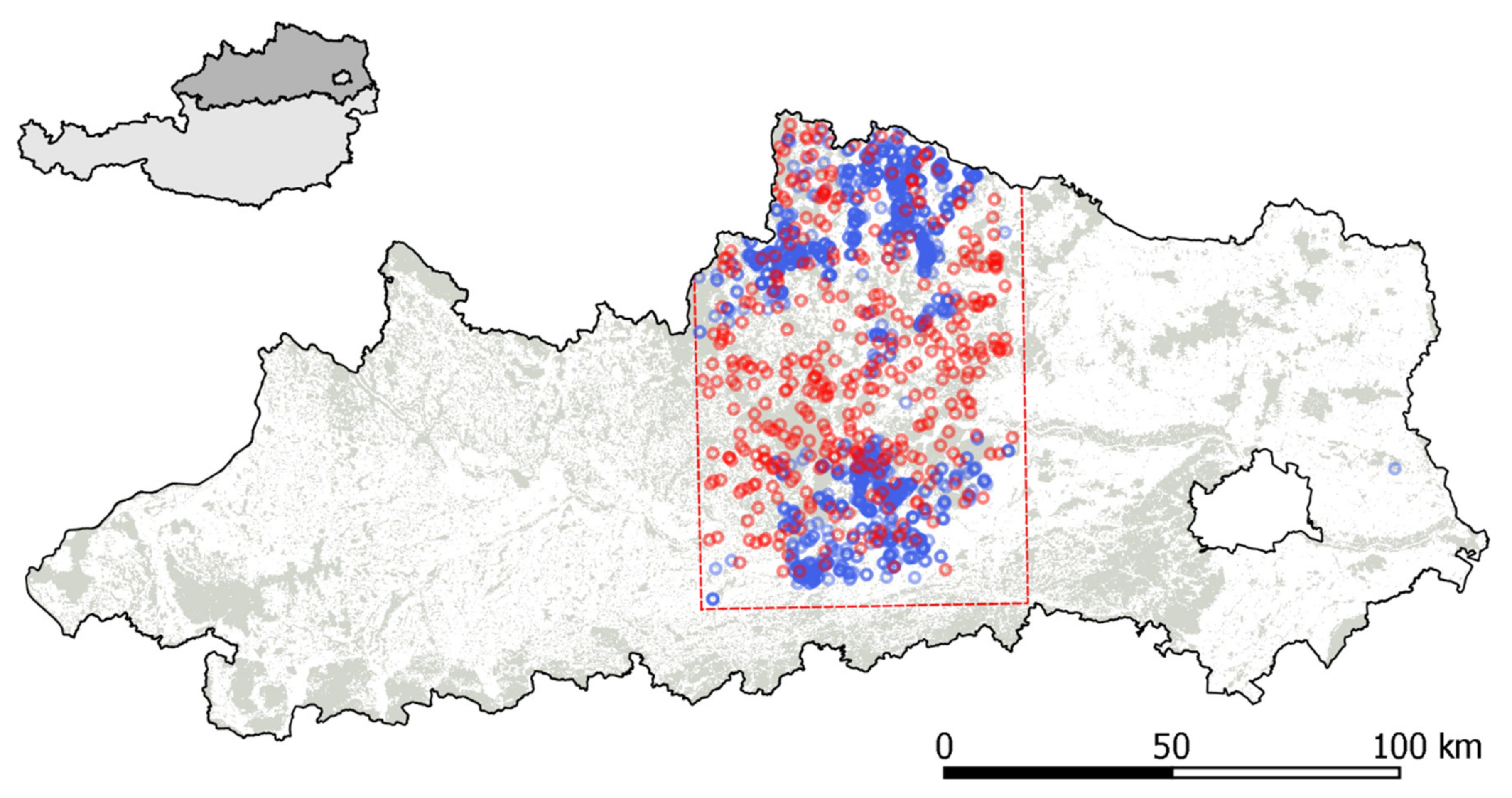
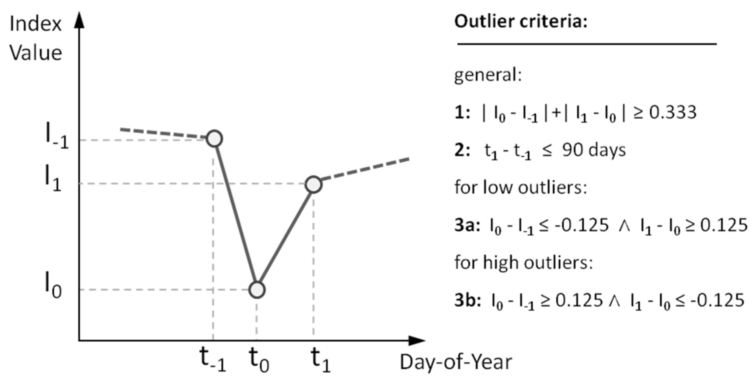
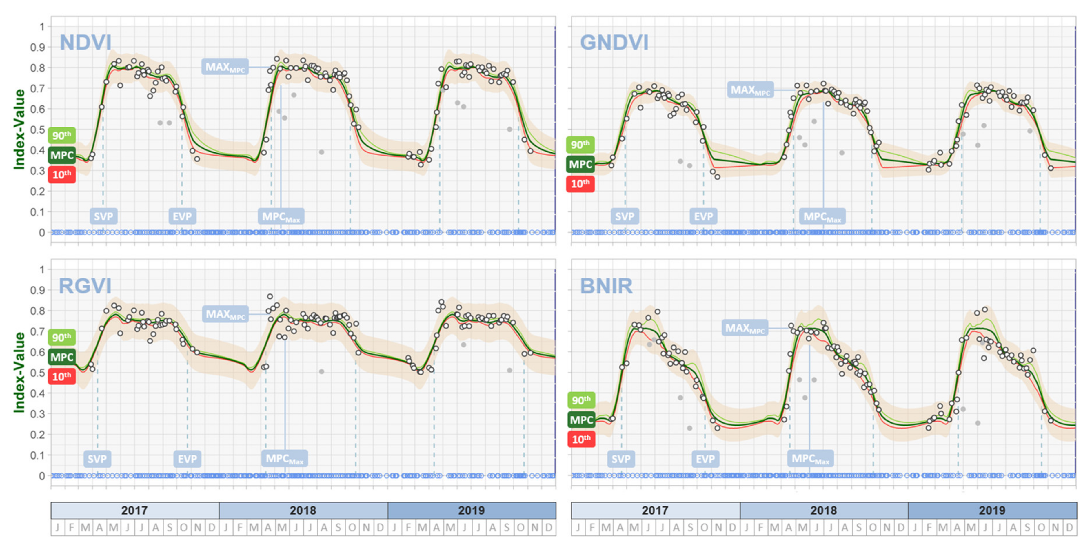
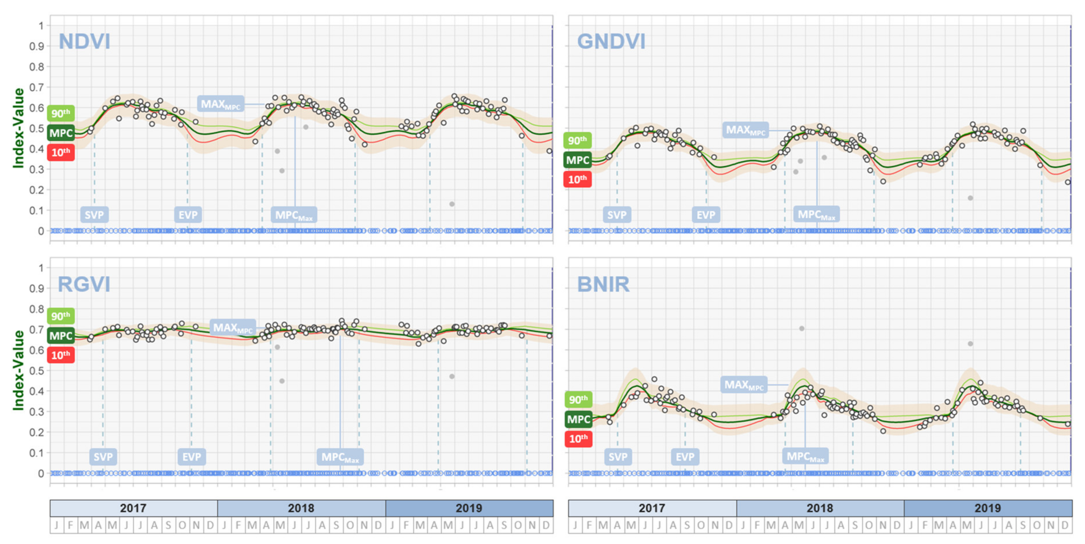
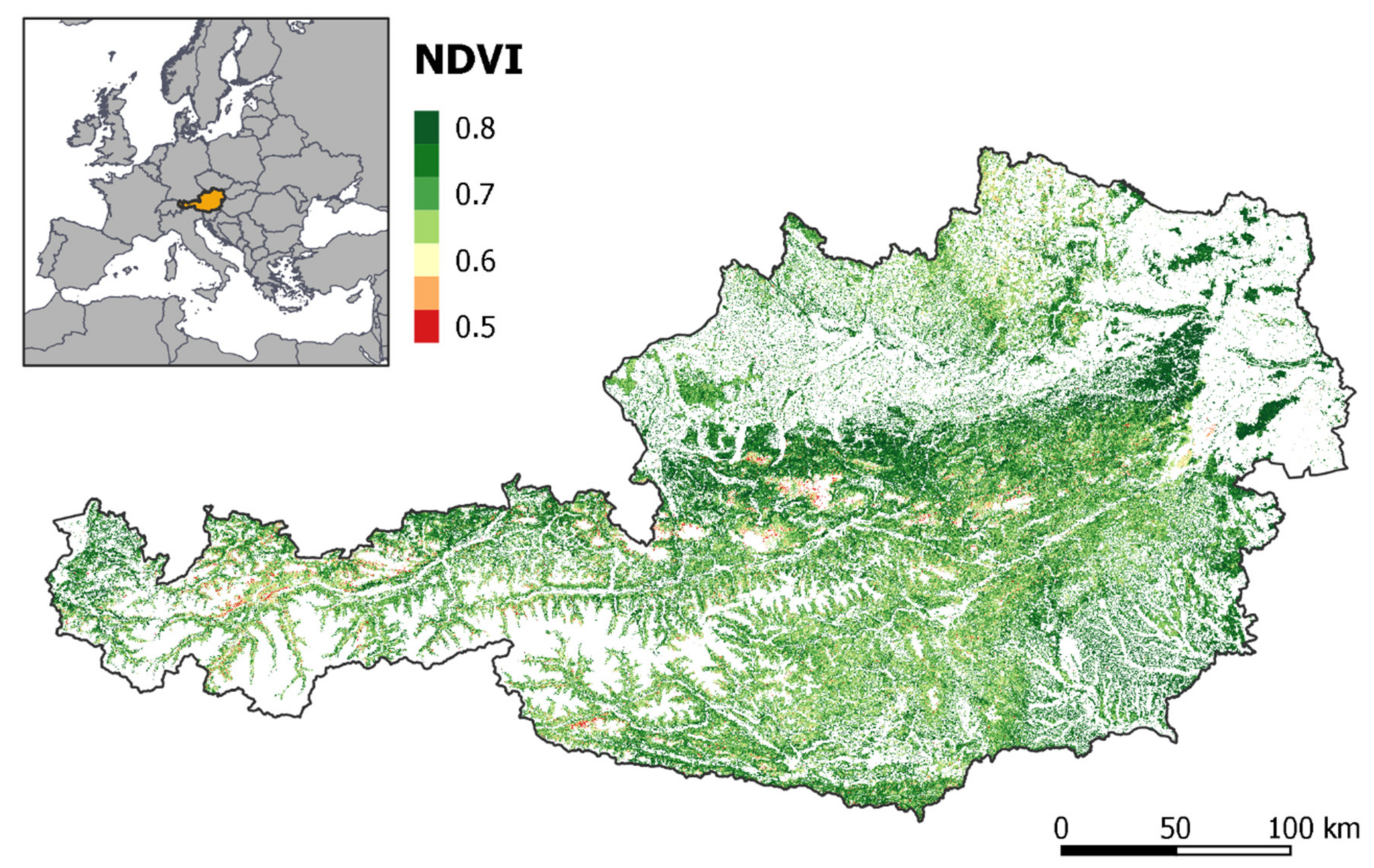
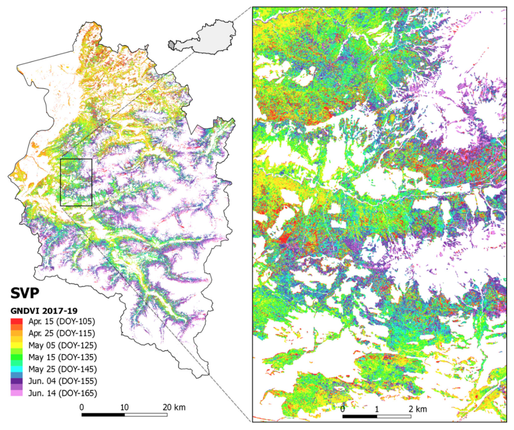
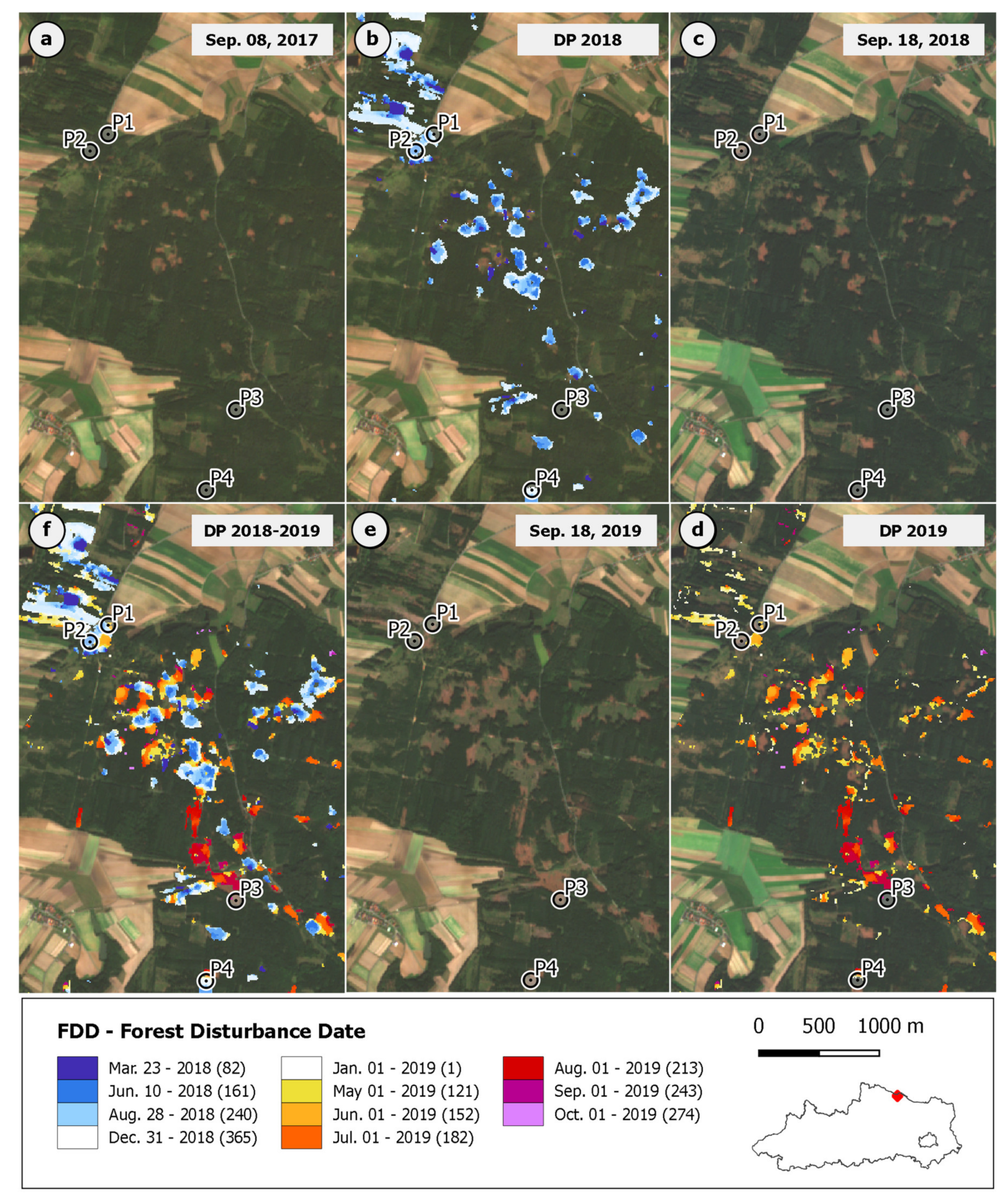
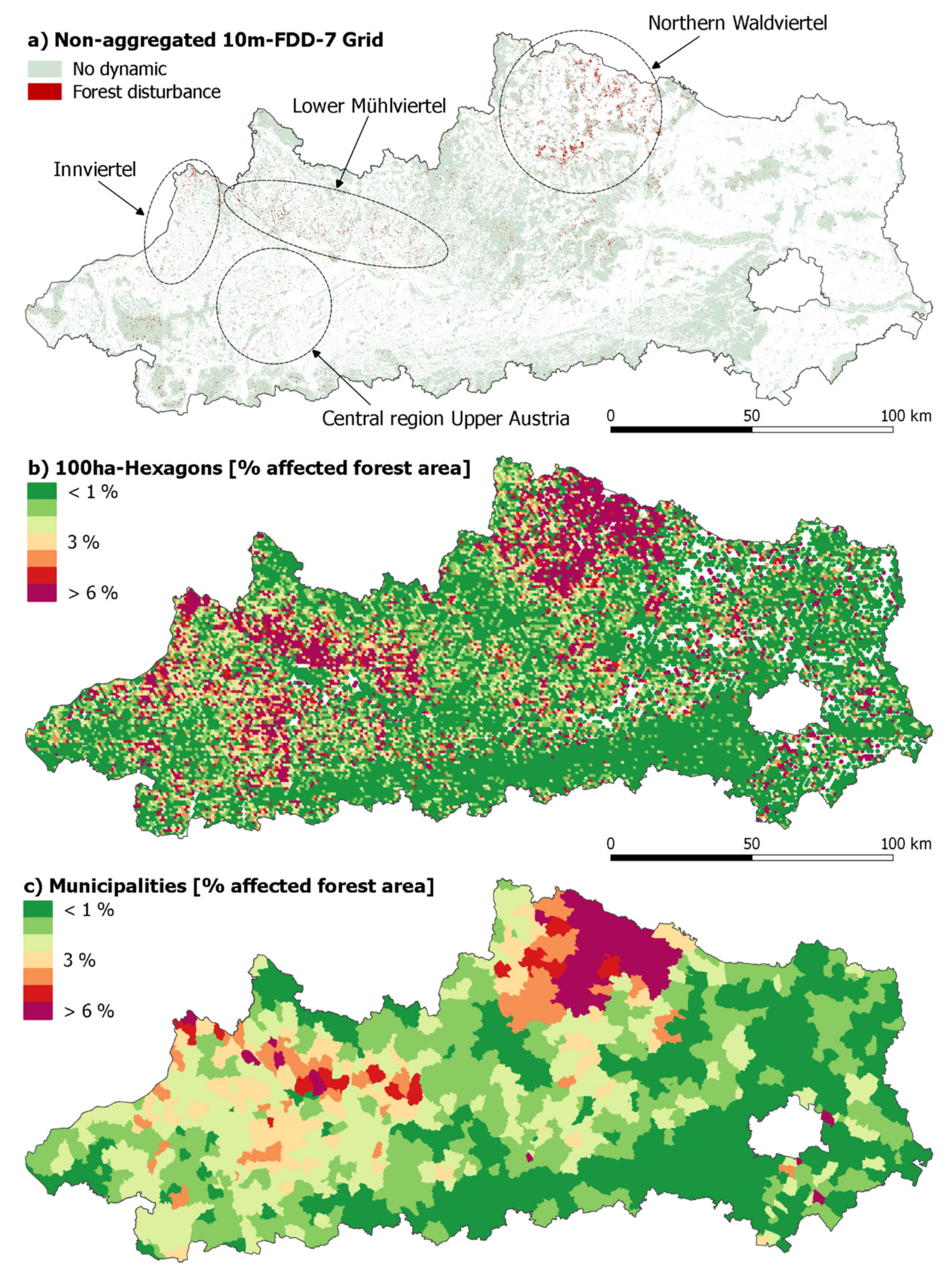
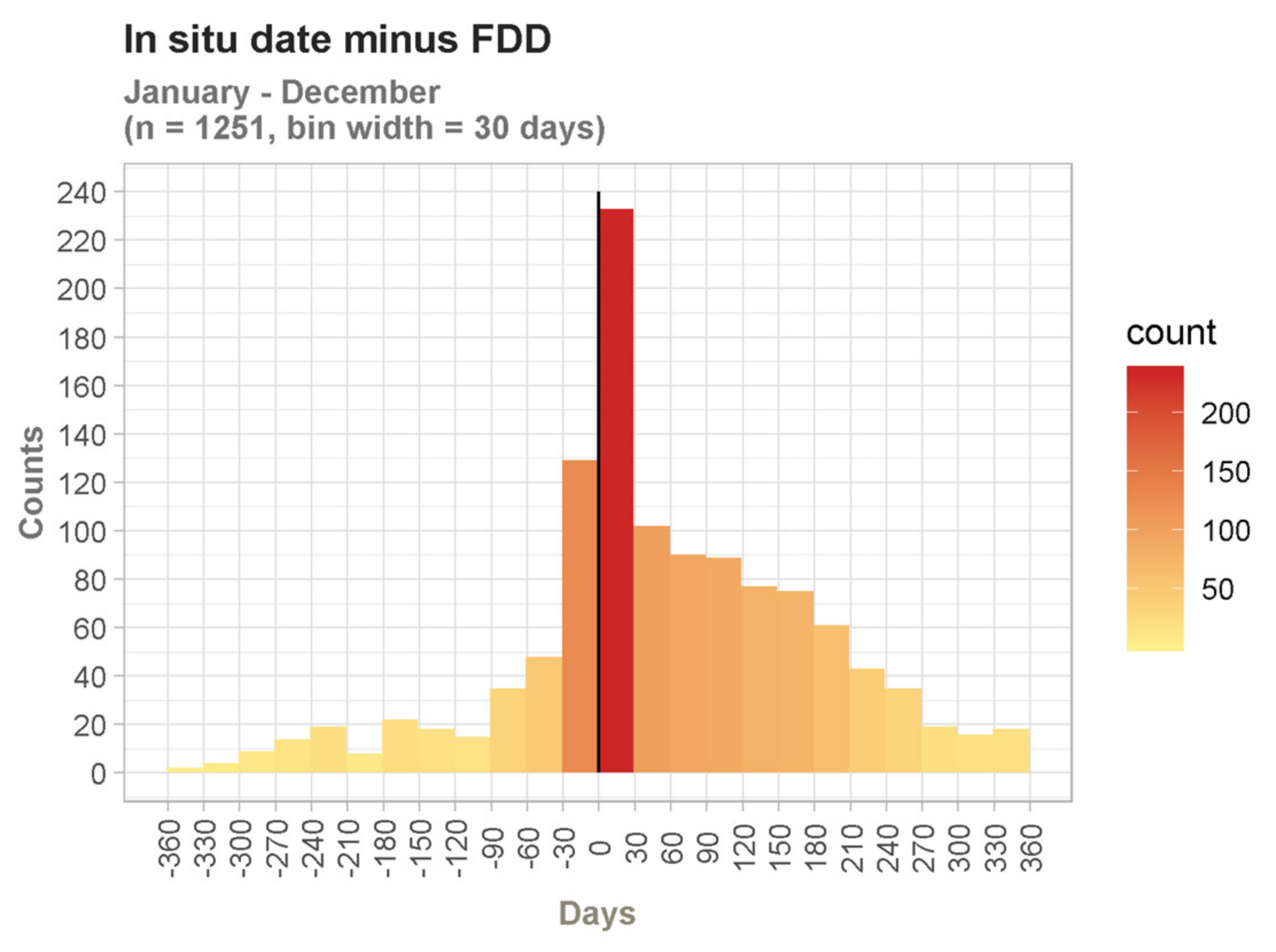
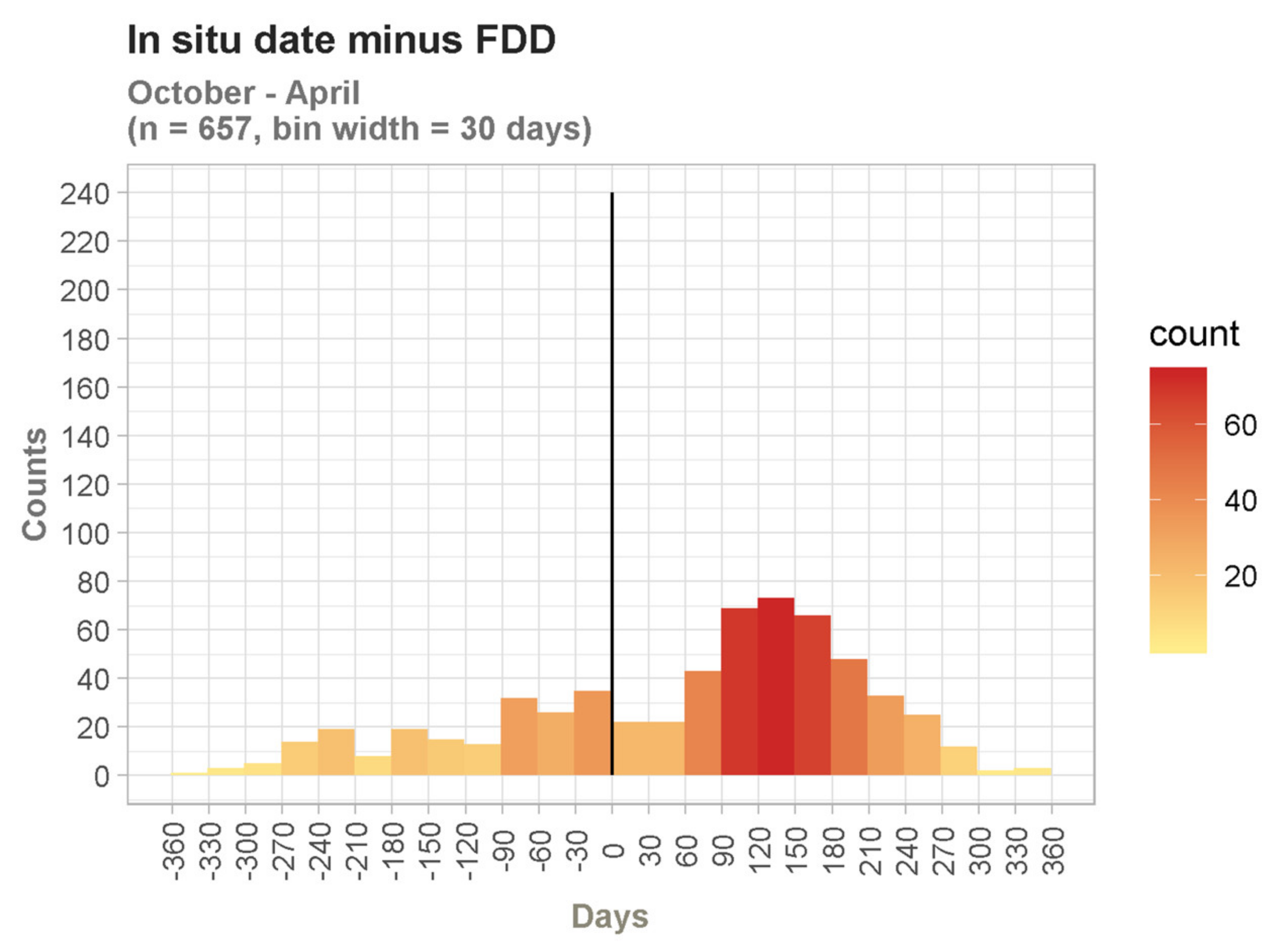
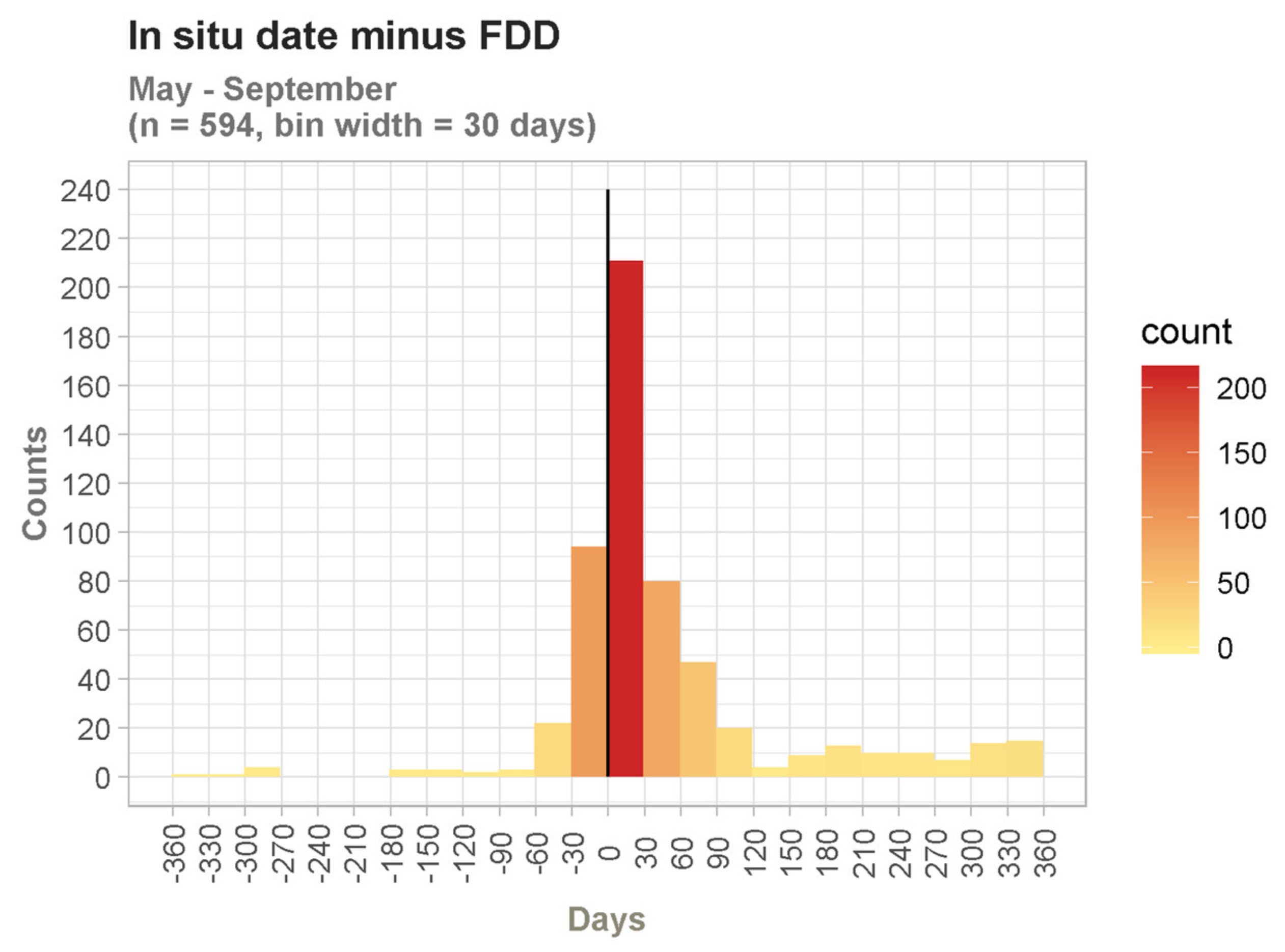
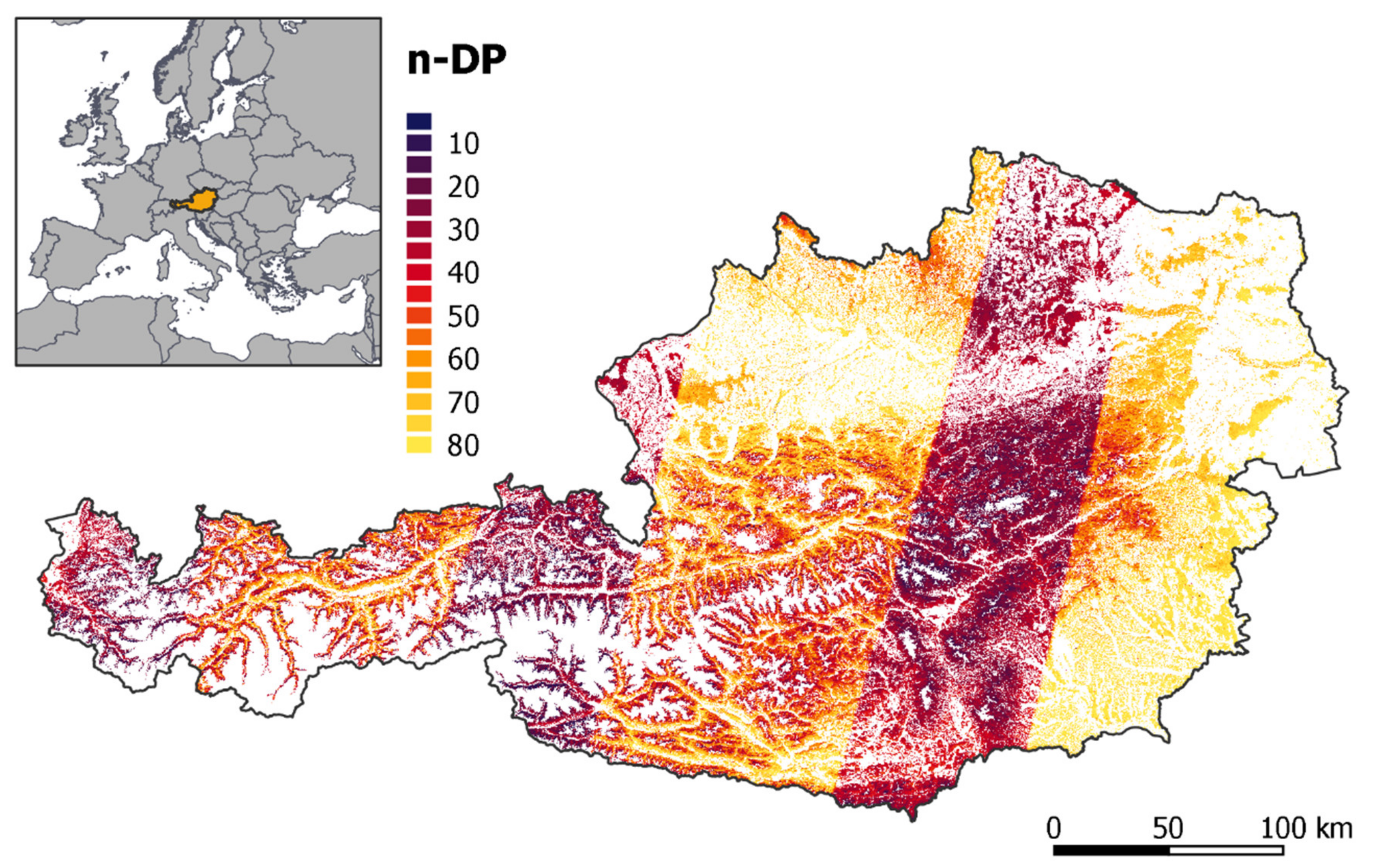
Table 1.
Spectral indices used in the study.
| Index | Name | Equation | Reference |
|---|---|---|---|
| NDVI | Normalised Difference Vegetation Index | [41] | |
| GNDVI | Green Normalised Difference Vegetation Index | [42] | |
| RGVI | Red-Green-Vegetation Index | + 0.5 | [43], edited |
| BNIR | Band: Near Infrared | own equation |
Table 2.
Savitzky-Golay-Filtering (SGF) settings used in the study.
| Parameter | Model Period | Detection Period |
|---|---|---|
| Degree of polynomial function | 3 | 2 |
| Window type | dynamic | fixed |
| Window size (days) | 31 | |
| Minimum window size (days) | 31 | - |
| Maximum window size (days) | 122 | - |
Table 3.
Validation results of the FDD grid.
| Reference Dataset | Disturbance (Count) | No Disturbance (Count) | Disturbance (Fraction) | No Disturbance (Fraction) |
|---|---|---|---|---|
| In situ dataset for class “Disturbance” | 1251 | 249 | 83.4% | 16.6% |
| Random sample dataset for class “No Disturbance” | 13 | 258 | 4.8% | 95.2% |
Publisher’s Note: MDPI stays neutral with regard to jurisdictional claims in published maps and institutional affiliations. |
© 2020 by the authors. Licensee MDPI, Basel, Switzerland. This article is an open access article distributed under the terms and conditions of the Creative Commons Attribution (CC BY) license (http://creativecommons.org/licenses/by/4.0/).
Share and Cite
MDPI and ACS Style
Löw, M.; Koukal, T. Phenology Modelling and Forest Disturbance Mapping with Sentinel-2 Time Series in Austria. Remote Sens. 2020, 12, 4191. https://0-doi-org.brum.beds.ac.uk/10.3390/rs12244191
AMA Style
Löw M, Koukal T. Phenology Modelling and Forest Disturbance Mapping with Sentinel-2 Time Series in Austria. Remote Sensing. 2020; 12(24):4191. https://0-doi-org.brum.beds.ac.uk/10.3390/rs12244191
Chicago/Turabian StyleLöw, Markus, and Tatjana Koukal. 2020. "Phenology Modelling and Forest Disturbance Mapping with Sentinel-2 Time Series in Austria" Remote Sensing 12, no. 24: 4191. https://0-doi-org.brum.beds.ac.uk/10.3390/rs12244191
Note that from the first issue of 2016, this journal uses article numbers instead of page numbers. See further details here.