Using Earth Observation for Monitoring SDG 11.3.1-Ratio of Land Consumption Rate to Population Growth Rate in Mainland China

Abstract

Urban sustainable development has attracted widespread attention worldwide as it is closely linked with human survival. However, the growth of urban areas is frequently disproportionate in relation to population growth in developing countries; this discrepancy cannot be monitored solely using statistics. In this study, we integrated earth observation (EO) and statistical data monitoring the Sustainable Development Goals (SDG) 11.3.1: “The ratio of land consumption rate to the population growth rate (LCRPGR)”. Using the EO data (including China’s Land-Use/Cover Datasets (CLUDs) and the Defense Meteorological Satellite Program/Operational Linescan System (DMSP/OLS) nighttime light data) and census, we extracted the percentage of built-up area, disaggregated the population using the geographically weighted regression (GWR) model, and depicted the spatial heterogeneity and dynamic tendency of urban expansion and population growth by a 1 km × 1 km grid at city and national levels in mainland China from 1990 to 2010. Then, the built-up area and population density datasets were compared with other products and statistics using the relative error and standard deviation in our research area. Major findings are as follows: (1) more than 95% of cities experienced growth in urban built-up areas, especially in the megacities with populations of 5–10 million; (2) the number of grids with a declined proportion of the population ranged from 47% in 1990–2000 to 54% in 2000–2010; (3) China’s LCRPGR value increased from 1.69 in 1990–2000 to 1.78 in 2000–2010, and the land consumption rate was 1.8 times higher than the population growth rate from 1990 to 2010; and (4) the number of cities experiencing uncoordinated development (i.e., where urban expansion is not synchronized with population growth) increased from 93 (27%) in 1990–2000 to 186 (54%) in 2000–2010. Using EO has the potential for monitoring the official SDGs on large and fine scales; the processes provide an example of the localization of SDG 11.3.1 in China.

1. Introduction

Urbanization, including urban expansion and demographic changes, is one of the most significant and irreversible effects of human population increase [1]. The worldwide increase in urban area has increased by 58,000 km² from 1970 to 2000, with an estimated increase of an additional 1,527,000 km² expected by 2030 [2]. Since the late 2000s, with the large-scale migration of the rural population to cities, the urban built-up area in China has grown by 78.5% while the urban population has grown by 46% [3]. The numbers show that human activities increase urban built-up area and urban population, speeding up the process of urbanization.

Both urban expansion and population growth produce certain benefits and challenges. Rapid urbanization has increased convenience in people’s daily lives, including more infrastructure and investment. Rapid population growth has increased the labor force and business opportunities and stimulates domestic demand. However, unplanned urban growth has created problems such as environmental pollution, traffic congestion, and water stress [4]. The excessive increase in population has intensified traffic pressure, poor living conditions, high unemployment rates, hunger, poverty, and resource shortages.

Furthermore, mutual interdependence and influence still exist between urban expansion and population change. With the massive flow of population into cities, the increase in population has driven urban expansion. As cities continue to expand, more rural people have moved to the cities, thereby accelerating urban expansion. The physical growth of urban areas is frequently disproportionate in relation to population growth. This discrepancy further results in less efficient land use in many forms, followed by expansion and encroachment of the built-up area on surrounding agricultural land. When the agricultural land is converted to built-up areas, reverse conversion is difficult. This discrepancy can result in an inadequate supply of urban resources due to the excessive population, as evidenced by the proportion of the urban population that lives in slums. Therefore, monitoring the speed of transition and area is necessary where growth is occurring spatially [5], and a plan for future city growth should be considered due to population growth.

The 17 sustainable development goals (SDGs), including 169 targets and 232 indicators, were designed to meet the ambitious goals of the millennium development goals (MDGs) that guide socially sustainable development [6]. SDG 11.3.1, defined as the ratio of the land consumption rate (LCR) to the population growth rate (PGR), is used to describe the relationship between urban expansion and demographic change. The LCR reflects the annual rate at which cities consume land for urbanized users, measures the compactness of cities, and represents the progressive expansion of urban space. Demographic change can be reflected by the PGR, which is the rate of population change caused by the natural population and migration in a given area over a unit period. The indicator reflects whether urban development is sustainable along a coordinated and orderly path (i.e., whether urban expansion keeps pace with population growth). SDG 11.3.1 not only assesses urban sustainable development, but also incorporates other indicators (e.g., SDGs 11.7.1, 11.2.1, 11.6, and 11.a.1).

The research on the SDG 11.3.1 indicator is still in an early stage with scarce related literature, and few reports released by various countries and organizations in relation to SDG 11.3.1. In the U.K. report [7], Wales’ LCR was 1.4% and PGR was 1.9%, and England’s LCR was 4.4% and PGR was 2.3%, from 2013 to 2016. During the same period, Scotland’s LCR rose by 6.1% while the PGR declined by 1.4%, which reveals sharply uneven land expansion and population growth in Scotland. The LCR in France grew by 1.4% and the PGR by 0.5% in 2006–2015 [8], which is significantly lower than in the U.K. Portugal’s LCR was 2.7% and the PGR was 0.04% from 2007 to 2015 [9]. The ratio of land consumption rate to the population growth rate (LCRPGR) of 194 global sample cities stratified according to world regions, city population ranges, and number of cities in the country groups, was 1.68 in 1990–2000 and 1.74 in 2000–2015, which are slight increases from the previous decade [10].

Except for Wales, existing reports show that urban growth being higher than population growth in the sample cities and countries reflect escalating inconsistency. However, existing reports concentrated on developed countries or sample cities, and developing countries in Africa, South America, and East Asia, have been neglected. The expansion of built-up areas was often carried out in an unplanned manner in developing countries, and administrations have been unable to keep track of growth-related processes. The natural population growth rate in developing countries is higher than that in developed countries. The contradiction between people and land is continuously increasing. China has been a developing country in the past few decades, and the coupling between urban expansion and demographic change in China has been neglected by researchers [4,11].

The SDG indicators were classified into three levels by Inter-Agency and Expert Group on SDG Indicators (IAEG-SDGs) according to the method and data availability. SDG 11.3.1 is listed as Tier II with explicit concepts, acknowledged formulas, and evaluation standards, but the data are hard to obtain. In the vast and sparsely populated Western China, some areas do not produce statistical data. Changes in administrative divisions result in statistical inconsistency, and earth observation (EO) can be used to obtain consistent data using the same data source and interpretation method, eliminating incomparability. More human, material, and financial resources are required for statistical data updates, whereas EO data updates are often less expensive. Therefore, for Tier II indicators, EO solutions have the ability to offset the lack of datasets, having wide coverage, high spatial resolution, strong timeliness, and a short acquisition period [12].

Monitoring SDG 11.3.1 can be disaggregated into two aspects: urban expansion and demographic change. For the first aspect, new options available through the use of remote sensing techniques can provide synoptic views in space and time for the periodic monitoring of the land that is or will be developed [13]. However, scientists have so far concentrated on megacities [14], eastern coastal regions [15], and the provincial cities [16] in mainland China. Using results from the local scale to determine China’s overall features is difficult [17]. Due to image acquisition and interpretation workloads, the expansion patterns of small and medium cities (accounting for 80% of all Chinese cities) have received less attention [18].

For the second aspect, determining the exact population within the extent of the built-up area defined in SDG 11.3.1, metadata was important because the built-up area expansion has increased the statistical scope of the urban residents. However, the population statistics data are usually collected by administrative regions, which are inconsistent with the boundaries of the built-up area in practical research (the built-up area is usually smaller than the administrative area), often causing the modifiable areal unit problem in geoscience research [19]. The population’s spatial distribution calculated by the average density of the region cannot reflect the spatial heterogeneity, and the accuracy does not meet the requirements of scientific research and engineering applications [20].

Therefore, the United Nations Human Settlements Programme (UN-HABITAT) Workshop emphasized the need for disaggregated population data when estimating the number of urban residents [21]; the best method recommended in SDG 11.3.1 metadata is to disaggregate the total population of the region in the form of a geographic grid to reveal the real spatial information in a census. A variety of remote sensing data can provide sources for population density data, such as night-time light [22], land use data [23], spectral reflectivity [24], and texture data [25]. Methods of population disaggregation, such as those based on pixel features [26], geostatistics [27], and interpolation methods [28], have been developed and widely used. However, due to the complex topography and large population in China, large-scale, long-term, and refined population density mapping is accompanied by challenges.

To address this knowledge gap, the built-up area and population density datasets were built and validated in mainland China from 1990 to 2010. Existing land use products were used to obtain area percentage of the built-up area at the grid level. The population was disaggregated to the grid level derived from EO and statistics. Moreover, the spatial heterogeneity and dynamic tendency of LCR, PGR, and LCRPGR in SDG11.3.1 metadata in 340 cities in mainland China were analyzed at 1 km × 1 km grids at city and national levels. Finally, the findings provide an example of the localization of SDG 11.3.1 in China.

The remainder of this paper is structured as follows: The data sources and methods are discussed in Section 2 and Section 3. The results are outlined in Section 4. A comparative analysis and the method validation are provided in Section 5, and Section 6 outlines the conclusions.

2. Data

2.1. Land Use/Land Cover (LULC) Data

Existing land use products from 1990, 2000, and 2010 in mainland China were used [5,29] in this paper (

Table 1. Data resources.

Datasets	Resolution	Time	Sources	Reference
LULC	30 m	1990, 2000, 2010	Data Centre for Resources and Environmental Sciences	http://www.resdc.cn/data.aspx?DATAID=99
Population	County	1990, 2000, 2010	The Fourth, Fifth, Sixth National Population Census, National Bureau of Statistics of China	http://www.stats.gov.cn/tjsj/pcsj/
DMSP/OLS	1 km	1992, 2000, 2010	National Oceanic and Atmospheric Administration	https://www.ngdc.noaa.gov/eog/dmsp/downloadV4composites.html
Administrative boundary map	County	2013	National Fundamental Geography Information System	http://www.ngcc.cn/ngcc/

). Land use/land cover (LULC) datasets were obtained by interpretation of Landsat Thematic Mapper/Enhanced Thematic Mapper (TM/ETM+) remote sensing data with a spatial resolution of 30 m and were derived from the China’s Land-Use/Cover Datasets (CLUDs) provided by the Data Centre for Resources and Environmental Sciences (RESDC). The construction land that we used included three types: urban construction land, rural construction land, and other construction land with classification accuracies exceeding 75%, representing the most accurate and long-term sequence of land use remote sensing monitoring products available for China [5].

2.2. DMSP/OLS Night-time Light Time Series

The Defense Meteorological Satellite Program/Operational Linescan System (DMSP/OLS) night-time light data were provided by the National Geographic Data Centre of the National Oceanic and Atmospheric Administration (NOAA), which quantitatively records the intensity of night-time light worldwide [30]. A continuity correction was performed, and the pixel overflow effect was eliminated before using the stable lights [31].

2.3. Census Data

The census data were provided by the National Bureau of Statistics of China. We selected county-level census data from 1990, 2000, and 2010. Due to changes in administrative divisions, the county-level census datasets across the 20-year period were inconsistent with county-level administrative boundaries. In order to match census datasets and the corresponding administrative boundary map, we revised the problem (i.e., the change of county range). For example, the Chongwen district of Beijing merged into the Dongcheng district of Beijing in 2010, which showed that the administrative boundary of Chongwen was merged spatially with Dongcheng. The census values of Dongcheng district and Chongwen district were separated before 2010. The population of the Chongwen district and Dongcheng district needs to be summarized as the total population of the Dongcheng district, corresponding to the administrative boundary map which was joined spatially.

3. Methods

3.1. SDG 11.3.1 Indicator

SDG 11.3.1 aims to monitor the coupling between the land expansion rate and the population growth rate in a given spatial extent and time period. UN-HABITAT issued a report that described detailed concepts and individual cases. The report used the urban built-up area to replace the urban agglomeration area and used the exact population range (within the built-up area) instead of the total population [21]. The SDG 11.3.1 indicators are calculated using the following formulas:

$${\mathrm{LCR}=\mathrm{Ln}(\mathrm{Urb}}_{\mathrm{t}+\mathrm{n}}{/\mathrm{Urb}}_{\mathrm{t}})/\mathrm{y}$$

(1)

$${\mathrm{PGR}=\mathrm{Ln}(\mathrm{Pop}}_{\mathrm{t}+\mathrm{n}}{/\mathrm{Pop}}_{\mathrm{t}})/\mathrm{y}$$

(2)

$$\mathrm{LCRPGR}=\mathrm{LCR}/\mathrm{PGR}$$

(3)

where Urb_t+n and Urb_t represent the built-up area in the final and initial years, respectively; Pop_t+n and Pop_t represent the urban residents within the built-up area in the final and initial years, respectively; and y is period span. Both LCR and PGR reflect the average annual growth rates.

LCR and PGR quantitatively describe the expansion intensity and demographic change in two phases. The higher the positive value, the larger the area of new growth, and vice versa. LCR < 0 indicates a built-up area decrease compared with the previous period, whereas LCR > 0 indicates an increase in the built-up area. Similarly, PGR > 0 indicates a population increase contrasted to the previous period; PGR < 0 indicates a population decrease, and the city is classified as a shrinking city, suggesting that the population and vitality are decreasing.

LCRPGR is the ratio of LCR to PGR. A LCRPGR < 0 indicates that either LCR or PGR is negative, but it is impossible to judge whether land or population is growing faster. When LCR and PGR are both positive, the LCRPGR value is greater than 0 and the LCRPGR value can be divided into two cases of LCRPGR > 1 and 0 < LCRPGR < 1. Therefore, in this case, we need to use the signs of LCR and PGR and define land growth type as LCRPGR > 1 or LCR > 0 and PGR < 0, and population growth type as 0 < LCRPGR < 1 or LCR < 0 and PGR > 0.

Ideally, the LCR should be synchronized with the PGR, indicating that the development of the two is coordinated. Then, according to the classification of SDG 11.3.1 provided by UN-HABITAT (

Table 2. The classification criteria proposed by UN-HABITAT.

City Urban Extent Density	LCRPGR Value
10–150 persons/hectare	<1: Efficient land use
	>1: Inefficient land use
151–250 persons/hectare	<1: Moving toward efficiency
	>1: Moving away from efficiency
>250 persons/hectare	<1: Insufficient land per person
	>1: Moving toward sufficient land per person

), the LCRPGR value is divided at the city level into 6 categories depending on the relationship between population density and the LCRPGR value [21]. Efficient land use, moving toward efficiency, and moving toward sufficient land per person in Table 2 indicate that the relationship between land use and population growth is coordinated, and the remaining three in Table 2 indicate that it is uncoordinated.

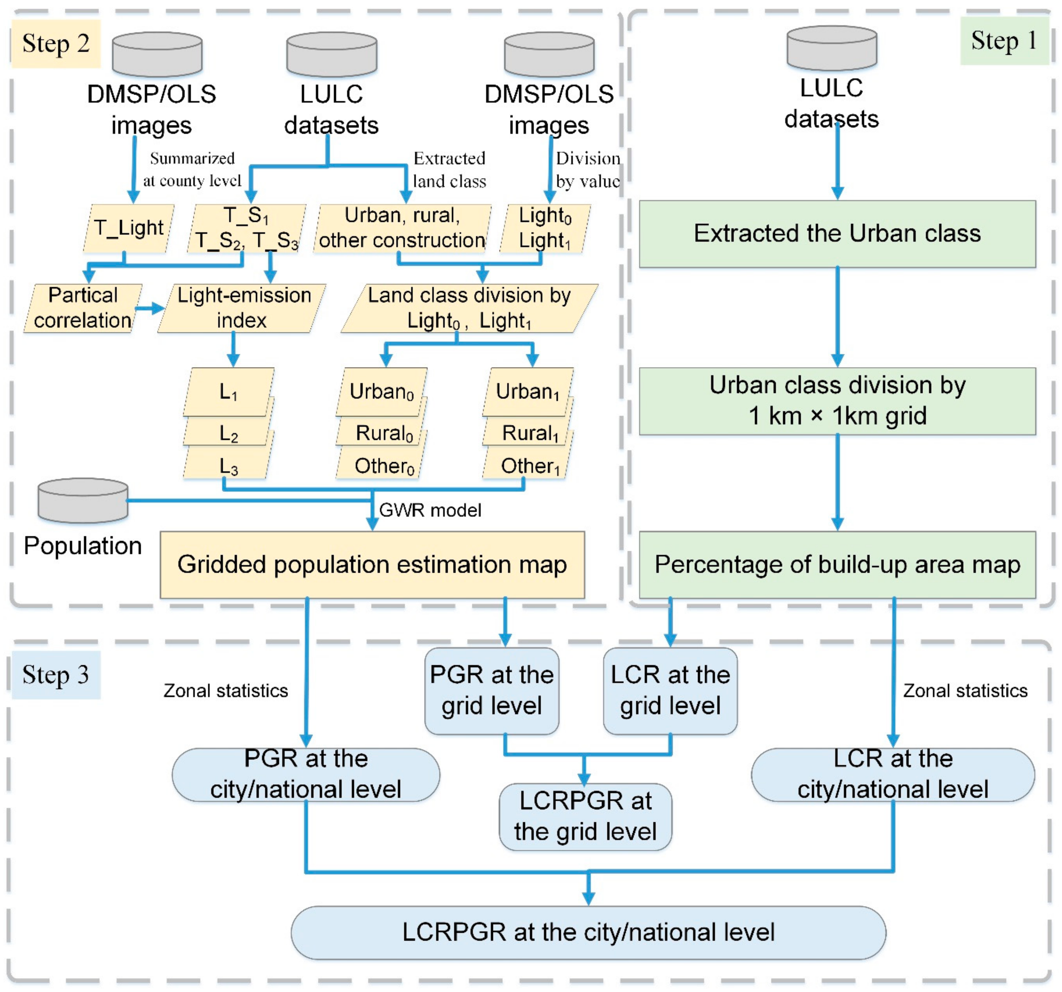
3.2. Calculation Process

The calculation process consisted of three major steps: (1) calculating the area percentage of built-up area in 1 km × 1 km grids, (2) disaggregating the population data at the 1 km × 1 km grid level, and (3) calculating the SDG11.3.1 indicator using Equations (1)–(3) in SDG 11.3.1 metadata. The flowchart is shown in Figure 1.

Step 1: The built-up areas were derived from urban construction land based on the definition (Section 5.3) of the built-up boundary that maintained the core area of the city, and we removed independent pixels (within 5 pixels), small areas at the edge of the city, and satellite cities [32]. Then, the extracted built-up area was divided into 1 km × 1 km grids, and the percentage of the built-up areas was calculated in each grid in mainland China from 1990 to 2010.

Step 2: To calculate population density, the area percentages of rural and other construction were calculated. Next, a refined resolution was obtained using a proposed model [27] to disaggregate the census data into 1 km × 1 km grids in mainland China over the 20 year period. Using the process in 1990 as an example, the specific steps were as follows (a–c):

(a) According to the light value of DMSP/OLS data, which was either zero or nonzero, the corrected DMSP/OLS data (called Light) were divided into two layers: Light₀ and Light₁. Three land class layers (urban, rural, and other construction land), were divided by the two layers (Light₀ and Light₁). Then, six layers were finally named: Urban₀ (urban class with light equal to 0), Urban₁ (urban class with light equal to 1), Rural₀, Rural₁, Other₀, and Other₁.

(b) The layers of Light and the area percentage data of urban, rural, and other construction land were summarized at the county level, called T_Light, T_S₁, T_S₂, and T_S₃, respectively. Then, the partial correlation coefficients were calculated between T_Light and T_S₁, T_S₂, and T_S₃, labeled F₁, F₂, and F₃, respectively. Next, L₁, L₂, and L₃ were calculated using Equation (4):

$${\mathrm{L}}_{\mathrm{j}}=\mathrm{Light}\frac{{\mathrm{T}\_\mathrm{S}}_{\mathrm{j}}{\times \mathrm{F}}_{\mathrm{j}}}{{{\displaystyle \sum }}_{\mathrm{j}}{\mathrm{T}\_\mathrm{S}}_{\mathrm{j}}{\times \mathrm{F}}_{\mathrm{j}}}$$

(4)

where L_j represents the light-emission index; Light is the corrected DMSP/OLS data; F_j is partial correlation coefficient; T_S_j is the area sum of urban, rural, and other construction land at the county level; and j has a value range of 1, 2, and 3.

(c) The nine independent variables (Urban₀, Urban₁, Rural₀, Rural₁, Other₀, Other₁, L₁, L₂, and L₃) were aggregated at the county level individually, and the dependent variable (census at the county level) was applied to the geographically weighted regression (GWR) model. Finally, the population density map was obtained at 1 km ×1 km grid level with model accuracies of 0.65, 0.74, and 0.79 at county levels in 1990, 2000, and 2010, respectively.

Step 3: According to the results of steps 1 and 2, the built-up area and population density datasets were obtained at the grid level. The area percentage of built-up area and population density were aggregated within the built-up extent at the city level, and the national LCRPGR was calculated similarly. Then, the LCR, PGR, and LCRPGR were calculated at the grid, city, and national levels.

3.3. City Sizes

To monitor the urbanization process, the classification of cities would be beneficial for subsequent analysis due to a large number of cities. Considering the characteristics of urban population change, the original division criteria are not suitable for current needs [33]. The 2010 report proposed new division criteria of cities more in line with our period. According to the division criteria [33], the 340 cities were divided into 5 sizes based on the urban populations within the built-up extent in 2010: (1) large megacities: >10,000,000; (2) megacities: 5,000,000–10,000,000; (3) large cities: 1,000,000–5,000,000; (4) medium cities: 500,000–1,000,000; and (5) small cities: <500,000. The whole list of 340 cities (divided into 5 sizes) is available for download in the Supplementary Materials (Table S1).

4. Results

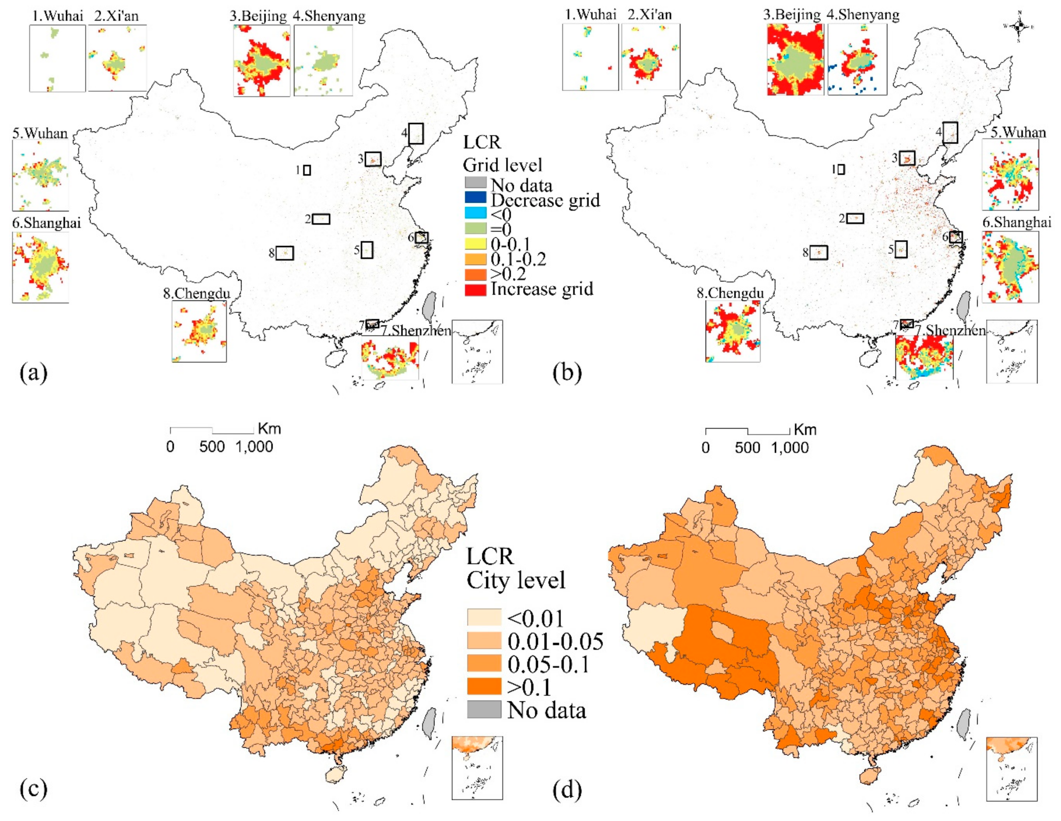
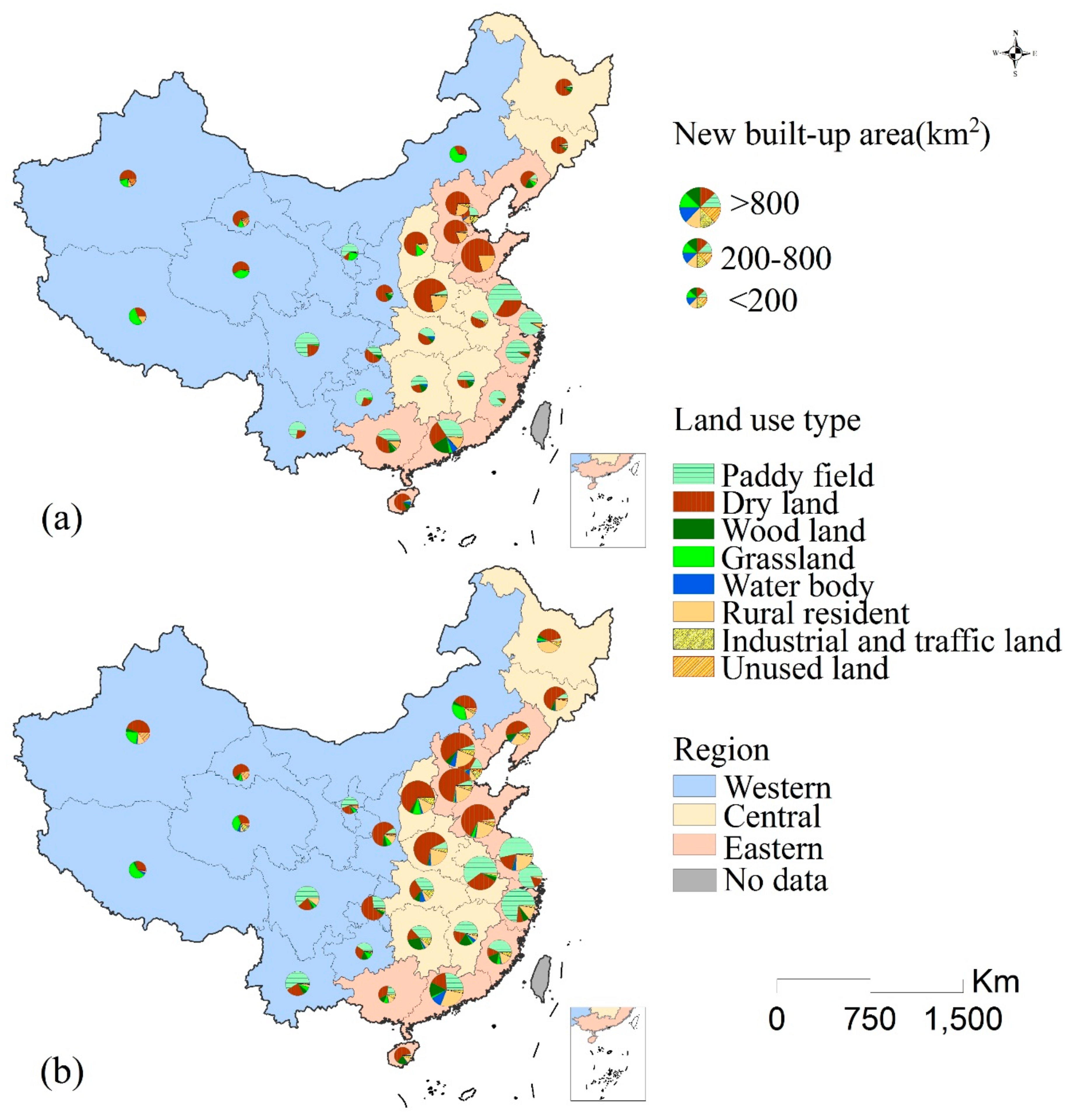
4.1. Spatial Expansion of the Built-Up Area

The LCR was used to quantify urban expansion (Figure 2a,b). At the grid level, the average LCR increased from 0.03 in 1990–2000 to 0.05 in 2000–2010, suggesting urban expansion in the two decades. The LCR value is not statistically significant, and we cannot say that it is a growing trend. The LCR value is low because LCR represents the annual rate at which cities uptake land for urbanized uses, and our measurement period is 10 years. Cities show higher LCR for the more recent decade than in the previous decade, suggesting that the urban expansion happened mostly in the first decade of the current century. The proportions of the grid that experienced a new increase (converted from other land types to construction land) were 13.7% and 41.7% during the periods of 1990–2000 and 2000–2010, respectively, indicating the built-up area encroached upon other land-use types. In the interior of the city, the LCR in large megacities increased from the center to the periphery, such as in Beijing city (Figure 2a,b). The LCR value in the urban center was zero, and the LCR values in the suburbs ranged from 0 to 0.2.

More than 95% of prefecture-level cities in China expanded in the two studied decades (Figure 2c,b). However, contrary to the inherent impression that the large megacities cities with the largest populations are expanding the fastest, more attention should be focused on the megacities (the second largest population size group), which demonstrated the most dramatic increase in intensity, with an average LCR of 0.13 from 1990 to 2010 (

Table 3. The average value of LCR and PGR.

City Size	LCR			PGR
	1990–2000	2000–2010	1990–2010	1990–2000	2000–2010	1990–2010
Large Megacities	0.049	0.064	0.113	0.071	0.047	0.118
Megacities	0.042	0.088	0.13	0.041	0.056	0.098
Large cities	0.026	0.062	0.088	0.022	0.044	0.066
Medium cities	0.023	0.049	0.072	0.006	0.04	0.047
Small cities	0.024	0.057	0.081	0.008	0.052	0.06

). Large megacities have an average LCR value of 0.11, which is slightly lower than that of megacities; large, medium, and small cities, with similar rates, have average values ranging from 0.72 to 0.88.

When disaggregated by region, the average LCR values in 1990–2000 were eastern (0.036) > western (0.028) > central (0.024), with growth areas of 5069, 1060, and 1823 km², respectively. The eastern region has advantages in terms of location, economy, and policy, whereas most western cities expanded slowly due to the sparse population, economic development, and a lack of infrastructure. In 2000–2010, the average LCR values were eastern (0.059) > western (0.042) > central (0.041), and the growth areas were 20,025, 3465, and 6489 km², respectively. Overall, the growing regions were concentrated along the eastern coast while the growth of the central and western regions was mainly reflected in the provincial capital cities.

Figure 3 depicts the proportion of other land types that were consumed by the newly increased built-up area at the provincial level. Paddy fields, dry land, rural residential, grassland, and woodland declined to different degrees. The proportion of dry land and paddy fields decreased in total from 77.2% to 65.8% during the period of 1990–2000 to 2000–2010, while the proportion of rural residential areas and other construction land increased in total from 10.4% to 18.6%. The decline in the proportion of agricultural land consumed by construction land is due to the protection outlined in China’s cultivated land policy that the total amount of cultivated land should be at least 1.8 billion acres, preventing the reduction of the amount of cultivated land by urbanization. As cities continue to spread, more land in suburbs and rural areas near suburbs has transformed into construction land, leading to more rural settlements being converted into construction land.

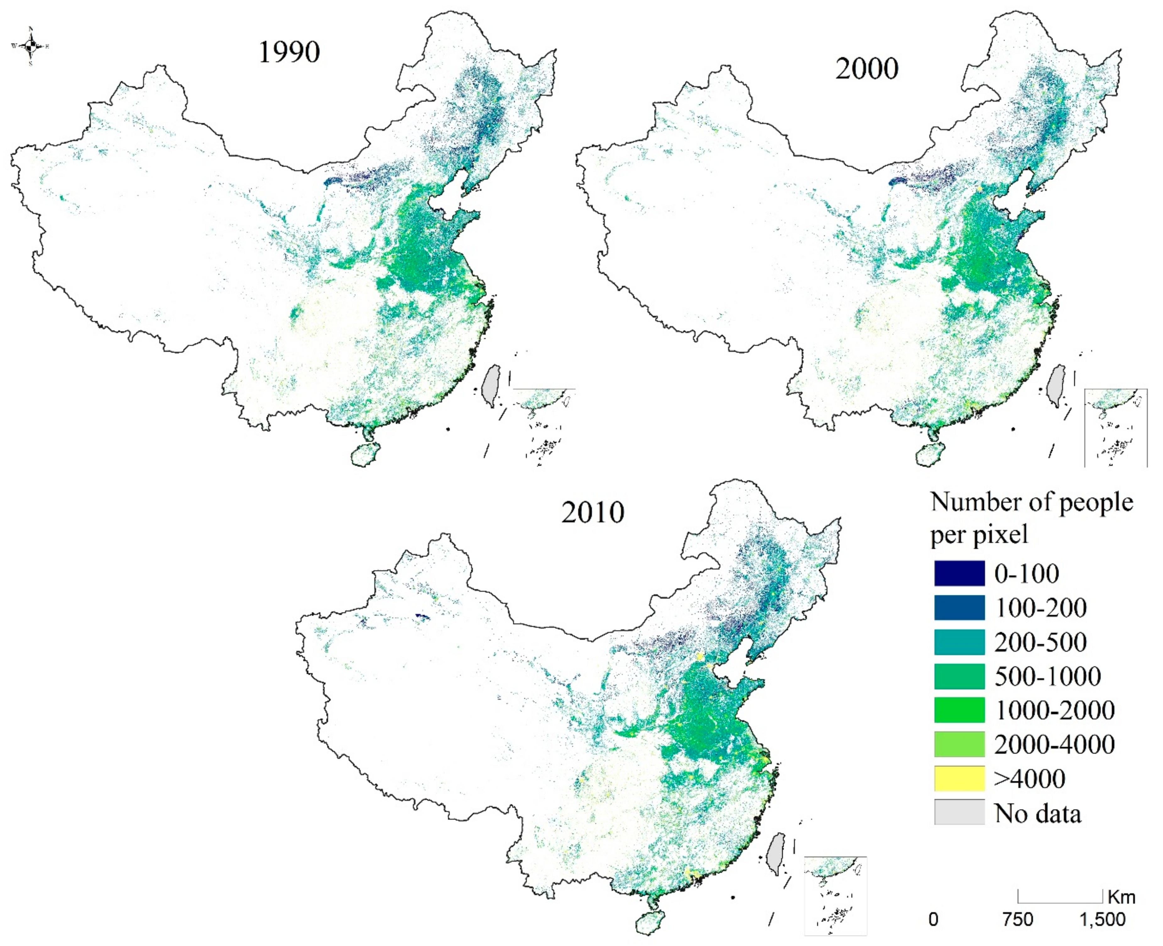
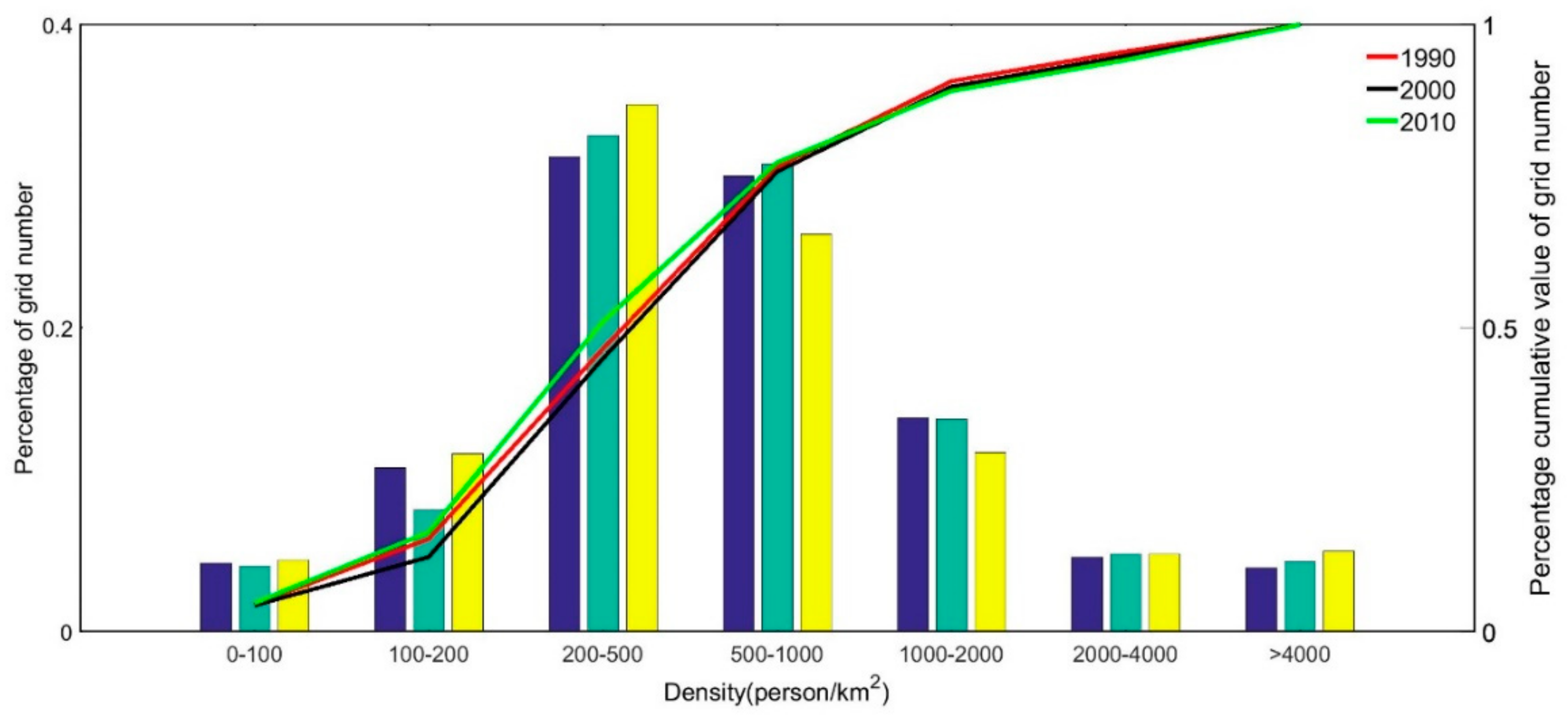
4.2. Spatiotemporal Dynamics of Population Density

Figure 4 shows that the population density in the large megacities and the Pearl River Delta in Southeast China was higher than 4000 people/km². The population in these areas accounted for 5% of the total population. The western region, which includes Xinjiang, Tibet, and Qinghai provinces, accounts for 40% of the total area, but the population accounts for only 2% of the total. The population distribution formed a dense spatial pattern in the low-elevation southeast areas, with sparse density in the northwest. As shown in Figure 5, the population density layers were divided into seven levels, of which the population density of 200–1000 people/km² has the highest share, containing approximately 70% of the total population. The proportion distribution of the population is similar to normal distribution.

The PGR was used to quantify demographic change (Figure 6a,b). At the grid level, the average PGR decreased from 0.004 in 1990–2000 to −0.010 in 2000–2010, showing a change from positive growth in the first period to negative growth in the second. Grids with a reduced proportion of the population accounted for 47% and 54% in the two periods, respectively. Despite the increase in total urban population, half of the grid showed a decrease in population density, and the PGR was relatively high in the remaining half of the grid, indicating an increase in the uneven population distribution.

We identified 112 shrinking cities with a population decline (PGR < 0) in 1990–2000 and 69 shrinking cities in 2000–2010 (Figure 6c,d). Shrinking cities were mainly concentrated in northeastern China in 1990–2000 and in 2000–2010 in southwestern China. The shrinking cities were mainly medium and small cities, but large megacities did not experience population decline. We highlight shrinking cities because the outcomes of the phenomenon may place pressure on urban vitality factors including transportation, housing, employment, public facilities, and other issues.

The average PGR values from 1990 to 2000 in the eastern, central, and western regions were 0.002, 0.010, and −0.004, respectively. In 2000–2010, the average values in the eastern, central, and western regions were −0.006, −0.011, and −0.018, respectively. The PGR in the central and western regions showed a downward trend reflected in the flow of the central and western populations to the eastern areas.

In terms of population mobility, the core peripheral effects reflected the population migration from the underdeveloped urban periphery to the core areas of economically developed urban agglomerations in the east, such as Beijing, Tianjin, and Hebei agglomeration. Provincial capitals in the central and western regions, such as Xi’an and Wuhan, as shown in Figure 6d, are strongly appealing to the population in surrounding urban, suburban, and rural settlements. The populations of small cities around the provincial capital cities were being seriously depleted.

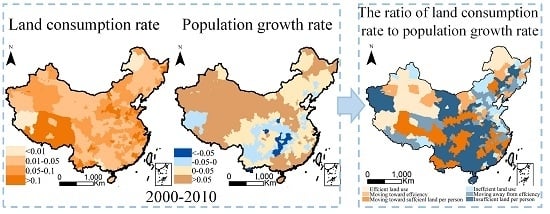
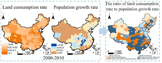
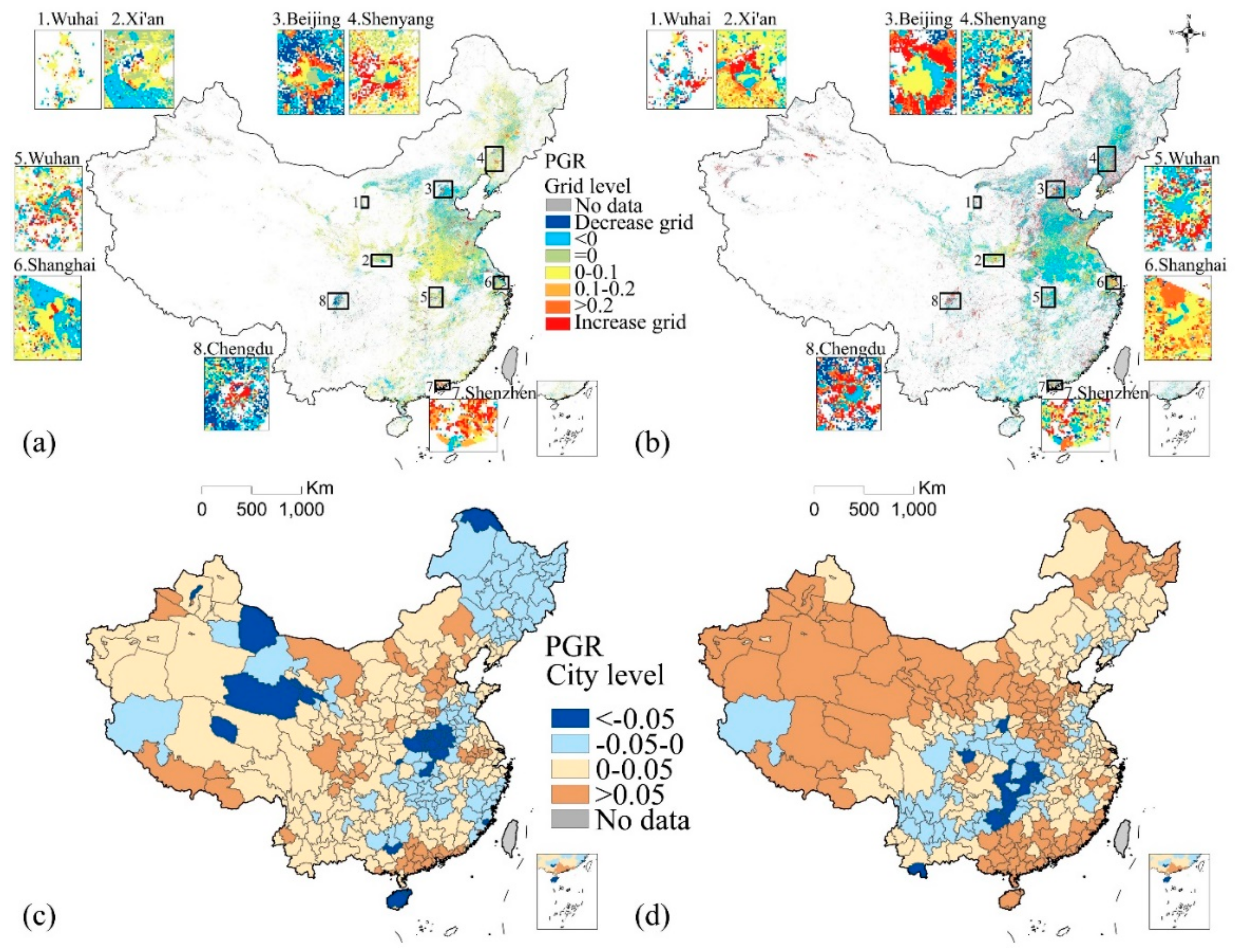
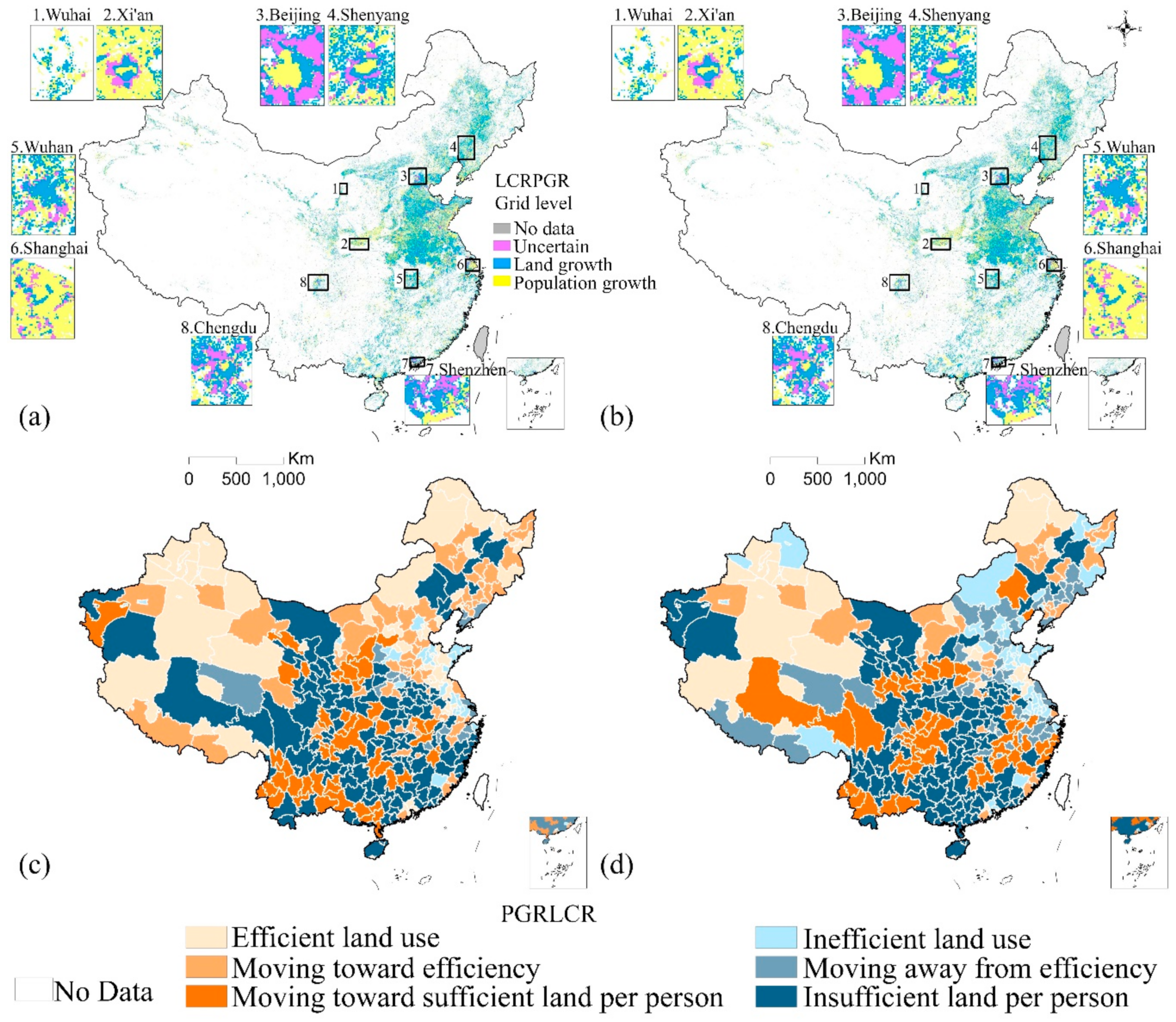
4.3. Spatial and Temporal Dynamic Changes in LCRPGR

Based on the grid level, the percentage of LCRPGR in 1990–2000 showed population growth (51%) > land growth (48%) > uncertain (1%) for the 1.15 million grids (Figure 7a). The population growth type was mainly distributed in developed cities or in underdeveloped rural areas because economically developed cities were positively affected by both natural population growth and mechanical growth (population migration), whereas the rural areas in the central and western areas had low LCR values during this period.

The percentage of LCRPGR type in 2000–2010 showed land growth (55%) > population growth (41%) > uncertainty (4%) for the 1.36 million grids (Figure 7b). The number of cities with land growth exceeded that with population growth type because urban development requires a large amount of land resources. In addition, based on geography and family membership, the household registration divided the population into a rural and urban population. Because migrants from rural to urban areas may not enjoy certain benefits, including schooling, employment, and medical, household registration restrictions impede the growth of the urban population. The number of land growth type is unlikely to decrease in a short period of time.

Table 4. The classification of the LCRPGR result.

LCRPGR Value		Number of Cities		Type
		1990–2000	2000–2010
LCRPGR > 1		93	154	Land growth type
0 < LCRPGR < 1		129	113	Population growth type
LCRPGR < 0	LCR > 0 & PGR < 0	112	69	Land growth type
	LCR < 0 & PGR > 0	6	4	Population growth type

shows that the number of cities experiencing land growth increased from 205 (60%) in 1990–2000 to 223 (65%) in 2000–2010, and the number of population growth type cities decreased from 135 (40%) in 1990–2000 to 117 (34%) in 2000–2010. During the period 1990–2010, the number of cities experiencing land growth type exceeded the population growth type cities.

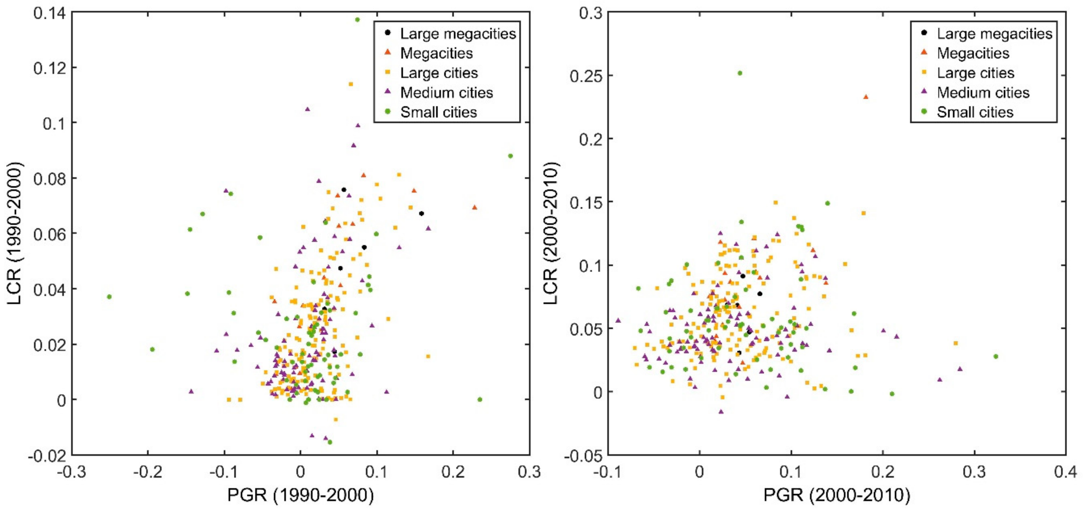
4.4. Coupling between LCR and PGR

Based on the division of UN-HABITAT, 247 (72%) cities were categorized as demonstrating coordinated development types and 93 (27%) cities as uncoordinated development in 1990–2000 (Figure 7c). In 2000–2010, 186 (54%) cities were categorized as demonstrating coordinated development types and 154 (45%) cities as uncoordinated development (Figure 7d). According to the UN-HABITAT standards, the number of uncoordinated cities has grown significantly to almost half of all cities, and the coordination relationship between LCR and PGR has deteriorated.

From the trend in LCR and PGR growth rates (Figure 8), first, although both the LCR and the PGR were positive in large megacities from 1990 to 2010, the LCR showed an upward trend, and the PGR decreased. Although the population of large megacities rose, the growth rate was slow. Then, both the LCR and the PGR of the megacities and large cities displayed growth trends, and the LCR growth rate was faster than the PGR rate in 1990–2010. Instead, the growth rates of the LCR in medium and small cities were significantly lower than the PGR rates in 1990–2010.

In 1990–2000, the correlation coefficient of LCR and PGR in 340 cities in mainland China was 0.35, whereas the correlation coefficient of LCR and PGR was 0.11 for all the cities from 2000 to 2010 at the 0.01 significance level. The significance test indicates that a relationship exists between LCR and PGR, but the low correlation coefficient indicates that the linear relationship between the LCR and PGR is very weak (Figure 9). The coupling between LCR and PGR is a complex nonlinear relationship.

5. Discussion

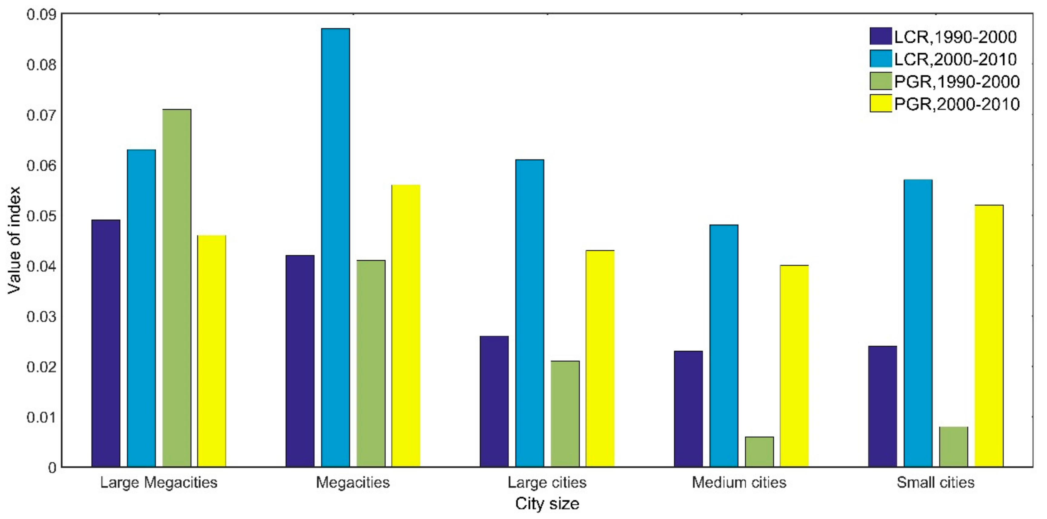
5.1. Analysis of LCR and PGR Change

More than 95% of the cities expanded from 1990 to 2010. The increase in the LCR was due to the city center being fully developed, and the suburbs provide the primary future reserve of urban development. More infrastructure and public resources shifted to the suburbs. Simultaneously, under the influence of compensation policy for cultivated land (the phenomenon of legal and paid occupation of rural land), cultivated land in the suburbs was converted into construction land. The cities presented a stall-style development model where the built-up area range is like many concentric circles, expanding outward and continuing to expand from the city center to the suburbs.

The population density decreased in half of the grids from 1990 to 2010. The decline in PGR was mainly due to the low birth rate (first, the number of women of childbearing age continued to decrease; second, the fertility rate was slightly lower than that in the previous period) and the outflow of the urban population. The urban population mainly flowed out from the west to the east; the population in underdeveloped urban areas flowed to developed urban agglomerations or provincial capital cities. The causes of population movements are complex. For example, passive population movements may be due to depletion of urban resources, while active population movements include migrants working outside the city. The decline of the urban population may cause shrinking in medium and small cities.

5.2. Comparisons with Previous Studies of Data and SDG 11.3.1 Indicator

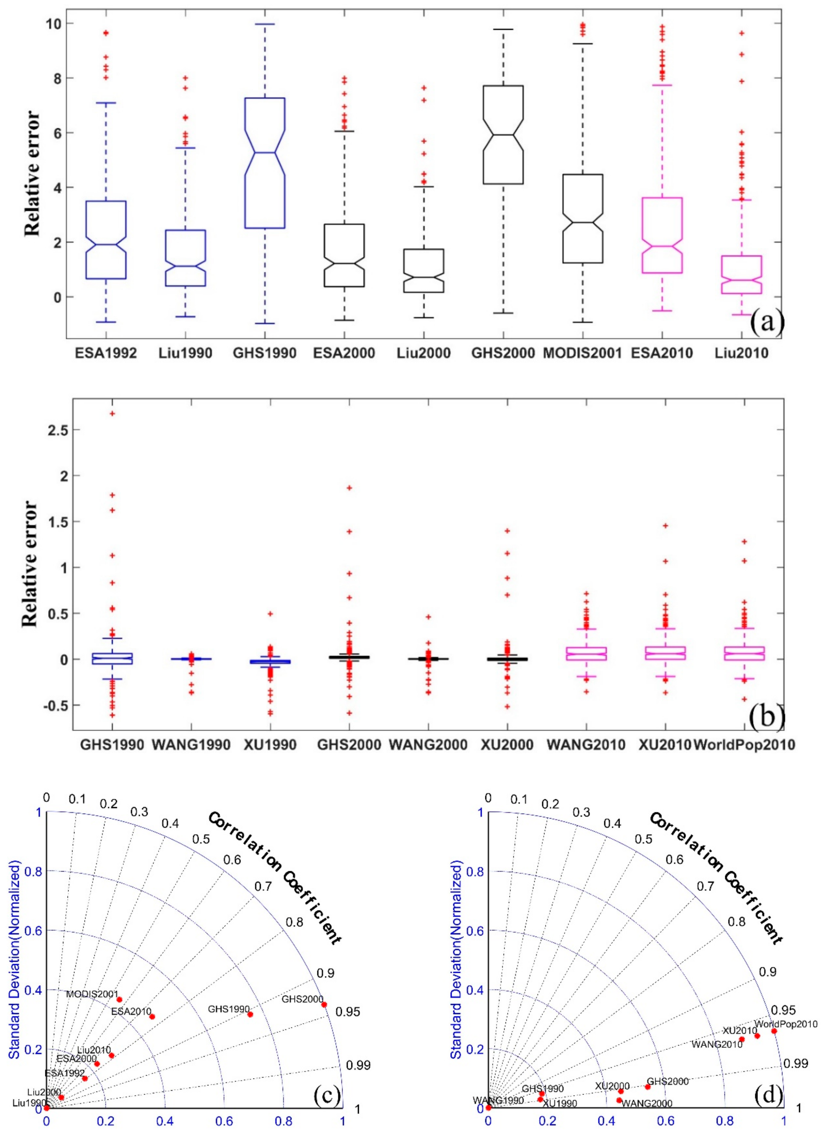
5.2.1. Comparisons with Previous Studies of Built-Up Area and Population Density Map

The built-up area and population density datasets were compared with other products and statistics (

Table 5. The data descriptions of other products.

	Products	Descriptions	Resolution	Reference
	Liu	Built-up areas in large, medium and small cities and above counties and towns	30 m	[29]
	ESA	Artificial surfaces and associated areas (urban areas >50%)	300 m	[34]
	GHS	The values representing the built-up area density ranging from 0 to 1	250 m	[35]
	MOD12Q1	At least 30% impervious surface area including building materials, asphalt, and vehicles	1 km	[36]
	Statistical data	Built-up area	City	https://kns.cnki.net/kns/brief/result.aspx?dbprefix=CYFD
Population	GHS	Estimates of numbers of people per pixel	1 km	[37]
	WorldPop		30″	[38]
	Xu		1 km	[39]
	Wang		1 km	This paper
	Census		County	http://www.stats.gov.cn/tjsj/pcsj/

) using evaluation criteria including the relative error, standard deviation, and correlation coefficients in our research area. Among them, Liu’s product [29] is the built-up area dataset used and Wang’s product is the population density map produced in this article.

First, we compared the relative error between the built-up area using statistical data and several products (Figure 10a). The relative error showed that the built-up area in the products was larger than the statistical value. The possible reasons for this finding are the following: (1) when the mixed pixels were decomposed, the end member abundance determined the possibility of misclassification; (2) nonvegetative land in the suburbs was easily interpreted as an urban built-up area [11], which increased the actual built-up area; and (3) parts of selected training samples, squares, parks, green spaces, and roads, which are limited by resolution, were often classified into built-up areas.

Among the four products (Figure 10a,c), Liu’s [29] has the highest spatial resolution of 30 m. We found that Liu’s relative error and standard deviation in three phases were the lowest. The correlation coefficients were approximately 0.8. In contrast, the relative error of the European Space Agency Climate Change Initiative (ESA CCI) [34] was larger with more extreme values, whereas Global Human Settlement (GHS) [35] had the highest relative error. The public land cover datasets (MCD12Q1 in MODIS products) [36] data are only suitable for monitoring the change in land-use after 2000. Therefore, Liu’s product [29] best met the requirements of large-scale and long-term sequences in our study area.

Second, we compared the accuracies of multiple population density products. No real measured 1 km × 1 km population density map exists in China. We chose an indirect method for verification as a compromise. We aggregated the population density products according to the administrative boundaries of prefecture-level cities and compared them with the census data using evaluation metrics, including the relative error, standard deviation, and the correlation coefficient.

As shown in Figure 10b, the relative errors of all products were close to zero. Overall, we found no obvious overestimation or underestimation. Among the four products, the relative errors of GHS [37] in 1990 and WorldPop [38] in 2010 were larger than those of the other products, with more extreme points and extensive distribution. The relative error distribution of Wang’s product produced in this article and Xu’s product [39] was more concentrated. In addition, Wang’s had fewer extreme data points and a smaller relative error; the standard deviation of Wang’s method was the lowest in these three time periods, and the correlation coefficient was high, within 0.95 to 1, as shown in Figure 10d. Finally, our population density map showed higher accuracy in our research area compared with the other population density datasets.

5.2.2. Comparisons with Previous Studies of LCR, PGR, and LCRPGR

The newly increased built-up areas in China increased by 37,950 km², while the urban population increased by 250 million in 1990–2010. For every additional city dweller, the newly built-up area increased by 151 m². In 1990–2015, the global newly built-up area increased by 255,000 km², while the urban population increased by 2 billion [40]. For every additional person in the global urban areas, the newly built-up area only increased by 102 m². This finding shows China is developing at the expense of land and needs to promote urban intensification.

China’s built-up area increased by 2.5 times, and the urban population increased by 1.7 times, from 1990 to 2010. Compared with previous research results, Wang et al. [4] reported that the built-up area had more than doubled in 1990–2010. Schneider et al. [11] found that from 1978 to 2010, China’s built-up area and population had been growing with a threefold increase in urban areas and a twofold increase in population. Our results showed that the increase in both built-up area and population and the growth rates aligned with the previously published results.

The LCR grew faster (1.8 times) than PGR from 1990 to 2010, with an LCR value of 0.09 and a PGR value of 0.05. Gao et al. [18] reported that China’s land expansion rate was higher than the population growth rate in 1990–2010; Nicolau et al. [9] found that Portugal’s land expansion has been faster than population expansion in the past few decades. A study of 10,000 selected urban centers worldwide showed that the urban land growth rate was 1.2 times greater than the population growth rate in 1990–2015 [40]. In this regard, China and many other countries are in a state of faster land expansion compared with population expansion.

China’s LCRPGR values were 1.69 and 1.78 during the 1990–2000 and 2000–2010 periods, respectively. The findings show that cities sampled in developed countries received LCRPGR values of 2.1 and 1.9 in 1990–¬¬¬2000 and 2000–2015, respectively; the LCRPGRs of 194 stratified sampling cities worldwide were 1.68 and 1.74 for the same periods [10]. Our values are closer to the global LCRPGR average value and lower than those of the developed countries because China’s urbanization is undergoing a period of formation. China’s urbanization processes are close to those of the United Kingdom in 1851, the United States in 1930, Japan in 1955, and South Korea in 1980. When China implemented the policy of reform and opening policy in 1978, the urban economy started developing. At present, China’s urbanization remains low, expressed by the industry and tertiary industry being constrained by factors such as institutions, markets, and industrial structure.

China’s LCR is higher than PGR in 1990–2010 at the national level. The number of cities with a land growth being higher than that of population growth shows that some built-up areas in cities have expanded too fast, exacerbating the imbalance. For example, the built-up areas in many southeast coastal cities increased more than threefold. We also found a small number of cities with higher LCRPGR (LCRPGR > 3)—19 (5%) cities in 1990–2000 and 47 (14%) cities in 2000–2010 indicating that LCR was much higher than the PGR in these cities, which reveals the need for more effective control of the intensity of urban expansion.

5.3. Uncertainty and Limitations

To assess the uncertainty of the SDG 11.3.1 indicator, we needed to evaluate the uncertainty of LCR with a focus on clear concepts, because the concept between a more semantic built-up area in the SDG and the classification in LULC products (Table 5) is heterogeneity. According to data from 231 cities around the world, 59% of built-up areas was composed of public space [41]. The key difference lies in the definition of public space, including parks, gardens, and roads. Public space impacts the estimation of the built-up area. However, no product can accurately estimate the built-up area due to inconsistent definitions and limited technology. As an alternative, many institutions and scholars adopted a compromise approach. For example, the U.K. used human-made surfaces [7] and France used artificial areas [8] as the built-up area. In practical applications, the classification of the LULC products relies more on data sources or training samples than on the semantic definition, resulting in a discrepancy when estimating built-up area boundaries [42]. We adopted the practical definition proposed by Song et al. [32], who retained the core area of the city and eliminated the rural areas in the periphery. Although the data differed from the metadata, our definition retained the content defined in the metadata to an extent and was suitable for calculation.

From the long-term, broad space, and multi-scale observations, we have learned the shortcomings of the LCRPGR indicator, including the following three points: (1) when the LCRPGR value is negative, it is not possible to rely solely on the LCRPGR value to reflect whether population or land has grown, so the sign of LCR and PGR is needed; (2) when the LCR and PGR values are both negative and LCRPGR > 1, the built-up area reduces faster than the population. In contrast, when the LCR and PGR values are both positive and LCRPGR > 1, the rate of urban expansion is faster than the rate of population growth. Here, it is also necessary to rely on the signs of LCR and PGR; and (3) the LCRPGR indicator is not suitable for identifying new growth construction land converted from other land types or for the built-up area or population that remained a constant value in a spatial unit and period span.

6. Conclusions

In this study, we monitored land-use efficiency, including the LCR, PGR, and LCRPGR proposed by the internationally agreed-upon methodology in SDG 11.3.1 metadata. The results were obtained by extracting the percentage of built-up area and disaggregating the population using the datasets derived from EO and statistical data, covering 340 prefecture-level cities in mainland China from 1990 to 2010. The spatial heterogeneity and dynamic tendency of urban expansion and population growth were explained at grid, city, and national levels, and were compared with the data from developed countries. We assessed the hypothesis that EO can be used for official SDG indicator monitoring in China. The major findings are as follows: (1) more than 95% of cities expanded from 1990 to 2010, especially in the megacities with populations of 5–10 million; (2) grids with a reduced proportion of the population accounted for 47% and 54% in the two periods, respectively; (3) the LCRPGR value of China increased from 1.69 to 1.78 during the period of 1990–2000 to 2000–2010, and the LCR was 1.8 times higher than the PGR in 1990–2010; and (4) the number of cities with uncoordinated development increased twofold from 93 (27%) to 186 (54%) between 1990–2000 and 2000–2010. Overall, the LCR is greater than the PGR, resulting in a one-third increase in the number of uncoordinated cities and a declining trend in land-use efficiency in 1990–2010.

We quantitatively described the characteristics of the land and population growth rates in five sizes of cities, which can provide a theoretical basis for land planning and population control. Our population datasets provide information for other indicators listed in the SDGs (e.g., poverty, health, education, energy, inequality, and climate change). The processes and evaluation criteria used in this article can be extended to other countries or regions, providing a reference for a unified comparison of the SDG 11.3.1. Our proposed method is not limited by data resolution, so globally available LULC and population density data can be used to calculate SDG11.3.1 indicators.

References

1. Grimm, N.B.; Faeth, S.H.; Golubiewski, N.E.; Redman, C.L.; Wu, J.; Bai, X.; Briggs, J.M. Global change and the ecology of cities. Science 2008, 319, 756–760. [Google Scholar] [CrossRef] [PubMed] [Green Version]
2. Seto, K.C.; Fragkias, M.; Gu, B.; Reilly, M.K. A Meta-Analysis of Global Urban Land Expansion. PLoS ONE 2011, 6, e23777. [Google Scholar] [CrossRef] [PubMed]
3. Bai, X.; Shi, P.; Liu, Y. Realizing China’s urban dream. Nature 2014, 509, 158–160. [Google Scholar] [CrossRef] [PubMed] [Green Version]
4. Wang, L.; Li, C.; Ying, Q.; Cheng, X.; Wang, X.; Li, X.; Hu, L.; Liang, L.; Yu, L.; Huang, H.; et al. China’s urban expansion from 1990 to 2010 determined with satellite remote sensing. Chin. Sci. Bull. 2012, 57, 2802–2812. [Google Scholar] [CrossRef] [Green Version]
5. Liu, J.; Liu, M.; Tian, H.; Zhuang, D.; Zhang, Z.; Zhang, W.; Tang, X.; Deng, X. Spatial and temporal patterns of China’s cropland during 1990–2000: An analysis based on Landsat TM data. Remote Sens. Environ. 2005, 98, 442–456. [Google Scholar] [CrossRef]
6. United Nations. Transforming our World: The 2030 Agenda for Sustainable Development; United Nations: New York, NY, USA, 2015; Available online: http://www.un.org/ga/search/view_doc.asp?symbol=A/RES/.70/1=E (accessed on 2 March 2019).
7. UK Office for National Statistics. Using Innovative Methods to Report against the Sustainable Development Goals. 2018. Available online: https://www.ons.gov.uk/economy/environmentalaccounts/articles/usinginnovativemethodstoreportagainstthesustainabledevelopmentgoals/2018-10-22 (accessed on 1 December 2018).
8. Commissariat General au Developpement Durable. Indicateurs Nationaux de la Transition Ecologique Vers Undeveloppement Durable (2015–2020); Commissariat General au Developpement Durable: Paris, France, 2016; Available online: http://www.statistiques.developpement-durable.gouv.fr/indi-cateurs-indices/f/.2491/0/artificialisation-sols-1.html (accessed on 1 December 2018).
9. Nicolau, R.; David, J.; Caetano, M.; Pereira, J. Ratio of Land Consumption Rate to Population Growth Rate—Analysis of Different Formulations Applied to Mainland Portugal. ISPRS Int. J. Geo. Inf. 2018, 8, 10. [Google Scholar] [CrossRef] [Green Version]
10. United Nations. The Sustainable Development Goals Report; United Nations: New York, NY, USA, 2016; Available online: https://www.un.org/development/desa/publications/sustainable-development-goals-.report-2016.html (accessed on 2 March 2019).
11. Schneider, A.; Mertes, C.M. Expansion and growth in Chinese cities, 1978–2010. Environ. Res. Lett. 2014, 9, 024008. [Google Scholar] [CrossRef]
12. Mariathasan, V.; Bezuidenhoudt, E.; Olympio, K.R. Evaluation of Earth Observation Solutions for Namibia’s SDG Monitoring System. Remote Sens. 2019, 11, 1612. [Google Scholar] [CrossRef] [Green Version]
13. Griffiths, P.; Hostert, P.; Gruebner, O.; der Linden, S.V. Mapping megacity growth with multi-sensor data. Remote Sens. Environ. 2010, 114, 426–439. [Google Scholar] [CrossRef]
14. Tian, G.; Jiang, J.; Yang, Z.; Zhang, Y. The urban growth, size distribution and spatio-temporal dynamic pattern of the Yangtze River Delta megalopolitan region, China. Ecol. Model. 2011, 222, 865–878. [Google Scholar] [CrossRef]
15. Liu, F.; Zhang, Z.; Shi, L.; Zhao, X.; Xu, J.; Yi, L.; Liu, B.; Wen, Q.; Hu, S.; Wang, X.; et al. Urban expansion in China and its spatial-temporal differences over the past four decades. J. Geogr. Sci. 2016, 26, 1477–1496. [Google Scholar] [CrossRef]
16. Wei, Y.; Zhao, M. Urban spill over vs. local urban sprawl: Entangling land-use regulations in the urban growth of China’s megacities. Land Use Policy 2009, 26, 1031–1045. [Google Scholar]
17. Tong, L.; Hu, S.; Frazier, A.E.; Liu, Y. Multi-order urban development model and sprawl patterns: An analysis in China, 2000–2010. Landsc. Urban Plann. 2017, 167, 386–398. [Google Scholar] [CrossRef]
18. Gao, B.; Huang, Q.; He, C.; Sun, Z.; Zhang, D. How does sprawl differ across cities in China? A multi-scale investigation using nighttime light and census data. Landsc. Urban Plann. 2016, 148, 89–98. [Google Scholar] [CrossRef]
19. Openshaw, S. A Million or so Correlation Coefficients: Three Experiments on the Modifiable Areal Unit Problem. In Statistical Applications in the Spatial Sciences; Wrigley, N., Ed.; Pion: London, UK, 1979; pp. 127–144. [Google Scholar]
20. Bai, Z.; Wang, J.; Yang, F. Research progress in spatialization of population data. Prog. Geogr. 2013, 32, 1692–1702. (In Chinese) [Google Scholar]
21. United Nations Human Settlements Program. Module 3: Land Consumption Rate. 2018. Available online: https://www.unescwa.org/sites/www.unescwa.org/files/u593/Module_3_land_consumption_edite586d_23-03-2018.pdf (accessed on 20 November 2018).
22. Lo, C.P. Modeling the population of China using DMSP operational linescan system nighttime data. Photogramm. Eng. Remote Sens. 2001, 67, 1037–1047. [Google Scholar]
23. Yuan, Y.; Smith, R.M.; Limp, W.F. Remodeling census population with spatial information from landSat TM imagery. Comput. Environ. Urban Syst. 1997, 21, 245–258. [Google Scholar] [CrossRef]
24. Lo, C.P. Automated population and dwelling unit estimation from high-resolution satellite images: A GIS approach. Int. J. Remote Sens. 1995, 16, 17–34. [Google Scholar] [CrossRef]
25. Liu, X.; Clarke, K.; Herold, M. Population density and image texture: A comparison study. Photogramm. Eng. Remote Sens. 2006, 72, 187–196. [Google Scholar] [CrossRef]
26. Azar, D.; Engstrom, R.; Graesser, J.; Comenetz, J. Generation of fine-scale population layers using multi-resolution satellite imagery and geospatial data. Remote Sens. Environ. 2013, 130, 219–232. [Google Scholar] [CrossRef]
27. Wang, L.; Wang, S.; Zhou, Y.; Liu, W.; Hou, Y.; Zhu, J.; Wang, F. Mapping population density in China between 1990 and 2010 using remote sensing. Remote Sens. Environ. 2018, 210, 269–281. [Google Scholar] [CrossRef]
28. Mennis, J. Generating surface models of population using dasymetric mapping. Prof. Geogr. 2003, 55, 31–42. [Google Scholar]
29. Liu, J.; Kuang, W.; Zhang, Z.; Xu, X.; Qin, Y.; Ning, J.; Zhou, W.; Zhang, S.; Li, R.; Yan, C.; et al. Spatiotemporal characteristics, patterns, and causes of land-use changes in China since the late 1980s. J. Geogr. Sci. 2014, 24, 195–210. [Google Scholar] [CrossRef]
30. Elvidge, C.D.; Sutton, P.C.; Ghosh, T.; Tuttle, B.T.; Baugh, K.E.; Bhaduri, B.; Bright, E. A global poverty map derived from satellite data. Comput. Geosci. 2009, 35, 1652–1660. [Google Scholar] [CrossRef]
31. Elvidge, C.D.; Sutton, P.C.; Baugh, K.E.; Ziskin, D.; Tilottama, G.; Anderson, S. National Trends in Satellite Observed Lighting: 1992–2009. AGU Fall Meet. Abstr. 2011, 3, 3. [Google Scholar]
32. Song, Y.; Huang, B.; Cai, J.; Chen, B. Dynamic assessments of population exposure to urban greenspace using multi-source big data. Sci. Total Environ. 2018, 634, 1315–1325. [Google Scholar] [CrossRef]
33. Compilation Committee of China’s Small and Medium-sized City Development Report. Small and Medium Cities Economic Development Committee of the Chinese Society of Urban Economics; Annual Report on Development of Small and Medium-Sized Cities in China (2010); Social Sciences Academic Press: Beijing, China, 2010; p. 23. [Google Scholar]
34. Defourny, P.; Bontemps, S.; Lamarche, C.; Brockmann, C.; Boettcher, M.; Wevers, J.; Kirches, G. Land Cover CCI: Product User Guide Version 2.0. 2017. Available online: http://maps.elie.ucl.ac.be/CCI/viewer/download/ESACCI-LC-PUG.-v2.0.7.pdf (accessed on 2 March 2019).
35. Pesaresi, M.; Ehrilch, D.; Florczyk, A.J.; Freire, S.; Julea, A.; Kemper, T.; Soille, P.; Syrris, V. GHS Built-Up Grid, Derived from Landsat, Multitemporal (1975, 1990, 2000, 2014). European Commission, Joint Research Centre (JRC). 2015. Available online: http://data.europa.eu/89h/jrc-ghsl-ghs_built_ldsmt_globe_r2015b (accessed on 2 March 2019).
36. Friedl, M.A.; Sulla-Menashe, D.; Tan, B.; Schneider, A.; Ramankutty, N.; Sibley, A.; Huang, X. MODIS Collection 5 global land cover: Algorithm refinements and characterization of new datasets. Remote Sens. Environ. 2010, 114, 168–182. [Google Scholar] [CrossRef]
37. European Commission, Joint Research Centre (JRC); Columbia University, Center for International Earth Science Information Network-CIESIN. GHS Population Grid, Derived from GPW4, Multitemporal (1975, 1990, 2000, 2015). European Commission, Joint Research Centre (JRC). 2015. Available online: http://data.europa.eu/89h/jrc-ghsl-ghs_pop_gpw4_globe_r2015a (accessed on 2 March 2019).
38. WorldPop (www.worldpop.org-School of Geography and Environmental Science, University of Southampton). China 100m Population. Alpha Version 2010, 2015 and 2020 Estimates of Numbers of People per Pixel (ppp) and People per Hectare (pph), with National Totals Adjusted to Match UN Population Division Estimates (http://esa.un.org/wpp/) and Remaining Unadjusted. 2015. Available online: http://0-doi-org.brum.beds.ac.uk/10.5258/SOTON/WP00055 (accessed on 3 March 2019).
39. Xu, X. China Population Spatial Distribution Kilometer Grid Dataset. Data Registration and Publishing System of Resource and Environmental Science Data Center of Chinese Academy of Sciences. 2017. Available online: http://www.resdc.cn/DOI/DOI.aspx?DOIid=32 (accessed on 2 March 2019). [CrossRef]
40. Marcello, S.; Michele, M.; Christina, C.; Aneta, J.F.; Sergio, F.; Martino, P.; Thomas, K. Multi-Scale Estimation of Land Use Efficiency (SDG 11.3.1) across 25 Years Using Global Open and Free Data. Sustainability 2019, 11, 5674. [Google Scholar]
41. United Nations. The Sustainable Development Goals Report. 2018. Available online: https://www.un.org/development/desa/publications/the-sustainable-development-goals-eport-2018.html (accessed on 4 March 2019).
42. Schneider, A.; Friedl, M.A.; Potere, D. A new map of global urban extent from MODIS satellite data. Environ. Res. Lett. 2009, 4, 044003. [Google Scholar] [CrossRef] [Green Version]
Figure 1. The flowchart of calculating SDG 11.3.1 (SDG: sustainable development goals; LCRPGR: The ratio of land consumption rate to population growth rate; LCR: land consumption rate; PGR: population growth rate).
Remotesensing 12 00357 g001
Figure 2. The LCR value in China in 1990–2010. (a,b) The spatial distribution of the LCR at 1 km × 1 km grid level; the increased grid indicates that the initial image has no built-up area in the grid and the final image has a built-up area in the grid, while the decrease grid means the opposite. (c,d) The spatial distribution of the LCR at the city level. (a,c) The LCR value in 1990–2000. (b,d) The LCR value in 2000–2010.
Remotesensing 12 00357 g002
Figure 3. The source of new built-up areas at the provincial level in China in 1990–2010.
Remotesensing 12 00357 g003
Figure 4. Population density maps with a 1 km × 1 km grid in 1990–2010.
Remotesensing 12 00357 g004
Figure 5. The area percentage of the grid number of population in 1990–2010. The histogram represents the area percentage of the grid number; the straight line represents the area percentage cumulative value of the grid number.
Remotesensing 12 00357 g005
Figure 6. The PGR value in China in 1990–2010. (a,b) The spatial distribution of the PGR at the 1 km × 1 km grid level; the increased grid indicates that the initial map has no population in the grid and the final image has a population in the grid, while the decrease grid means the opposite. (c,d) The spatial distribution of the PGR at the city level. (a,c) The PGR value in 1990–2000. (b,d) The PGR value in 2000–2010.
Remotesensing 12 00357 g006
Figure 7. The LCRPGR valued in China in 1990–2010. (a,b) The spatial distribution at the 1 km × 1 km level. The data sources of uncertain type included an increase/decrease grid when calculating the LCR and PGR, which cannot calculate the LCRPGR value according to Formula (3). (c,d) The spatial distribution at the city level. The orange legend shows that the relationship between the LCR and PGR tends to be effective and shows coordinated development, while the blue legend indicates that the relationship tends to be ineffective and uncoordinated and should be considered. The darker the orange and blue legends are, the greater the population density of the city is. (a,c) The LCRPGR value in 1990–2000. (b,d) The LCRPGR values in 2000–2010.
Remotesensing 12 00357 g007
Figure 8. The average LCR and PGR in 1990–2010.
Remotesensing 12 00357 g008
Figure 9. The scatter plots of LCR and PGR in 1990–2010.
Remotesensing 12 00357 g009
Figure 10. Statistical information on built-up area and population products at prefecture-level city scales in 1990–2010. Among them, (a,b) are the relative errors, and (c,d) are the normalized standard deviations and correlation coefficients.
Remotesensing 12 00357 g010