Evaluation of Evapotranspiration for Exorheic Catchments of China during the GRACE Era: From a Water Balance Perspective


1
School of Geography and Information Engineering, China University of Geosciences (Wuhan), Wuhan 430078, China
2
Artificial Intelligence School, Wuchang University of Technology, Wuhan 430223, China
3
State Key Laboratory of Geodesy and Earth’s Dynamics, Institute of Geodesy and Geophysics, Chinese Academy of Sciences, Wuhan 430077, China
4
College of Earth and Planetary Sciences, University of Chinese Academy of Sciences, Beijing 100049, China
5
School of Environment, Beijing Normal University, Beijing 100875, China
6
Department of Navigation Engineering, Naval University of Engineering, Wuhan 430033, China
*
Author to whom correspondence should be addressed.
Remote Sens. 2020, 12(3), 511; https://0-doi-org.brum.beds.ac.uk/10.3390/rs12030511
Submission received: 18 December 2019
/
Revised: 23 January 2020
/
Accepted: 4 February 2020
/
Published: 5 February 2020
(This article belongs to the Special Issue Remote Sensing of the Terrestrial Hydrologic Cycle)
Abstract
:Evapotranspiration (ET) is usually difficult to estimate at the regional scale due to scarce direct measurements. This study uses the water balance equation to calculate the regional ET with observations of precipitation, runoff, and terrestrial water storage changes (TWSC) in nine exorheic catchments of China. We compared the regional ET estimates from a water balance perspective with and without considering TWSC (ETWB: ET estimates with considering TWSC, and ETPQ: ET estimates from precipitation minus runoff without considering TWSC). Results show that the regional annual ET ranges from 417.7 mm/yr to 831.5 mm/yr in the nine exorheic catchments based on the water balance equation. The impact of ignoring TWSC on calculating ET is notable, as the root mean square errors (RMSEs) of annual ET between ETWB and ETPQ range from 12.0–105.8 mm/yr (2.6–12.7% in corresponding annual ET) among the exorheic catchments. We also compared the estimated regional ET with other ET products. Different precipitation products are assessed to explain the inconsistency between different ET products and regional ET from a water balance perspective. The RMSEs between ET estimates from Gravity Recovery and Climate Experiment (GRACE) and ET from land surface models can be reduced if the deviation of precipitation forcing data is considered. ET estimates from Global Land Evaporation Amsterdam Model (GLEAM) can be improved by reducing the uncertainty of precipitation forcing data in three semiarid catchments. This study emphasizes the importance of considering TWSC when calculating the regional ET using a water balance equation and provides more accurate ET estimates to help improve modeled ET results.

1. Introduction
Evapotranspiration (ET) is one of the most important components of the climate system connecting the water, energy, and carbon cycle [1,2]. ET changes can be used as an indicator of climate change, especially in areas where the water cycle is accelerated [3,4]. However, regional ET is often difficult to estimate. The flux tower observing station network can provide accurate ET observations at each site [5], but it often has too sparse sites for basin scale study. Remote sensing provides an opportunity to monitor spatial-temporal changes in ET [6,7], but regional calibration and uncertainty from vegetation cover data will also lead to large uncertainty in ET [8]. Land surface models (LSMs) can also provide grid-to-regional scale ET estimates, such as the multiple LSMs simulations using the global land data assimilation system (GLDAS) issued by NASA [9]. Regional ET can be derived from the terrestrial water budget, namely the residual between precipitation (P) and the sum of runoff (Q) and terrestrial water storage change (ds/dt), which have been regarded as benchmark estimates for validating ET products or estimates on a regional scale [10,11].
The Gravity Recovery and Climate Experiment (GRACE) satellites mission launched in March 2002 has provided a unique way to monitor terrestrial water storage (TWS) changes on the monthly scale with a ~300 km footprint [12]. As for a given basin, the time series of TWS changes (TWSC) in the basin can be obtained from the differential of TWS anomalies (TWSA) observed by GRACE [1,13,14]. The regional ET can be estimated from TWSC, regional precipitation, and runoff data based on the water balance equation. Rodell et al. [4] discussed the method of calculating ET from GRACE TWSA and suggested that the ET based on the GRACE water balance method can be used to evaluate the ET of the model simulations. Ramillien et al. [15] estimated the ET of 16 globally distributed basins based on the GRACE water balance method, and they are compared to outputs of four global LSMs, which shows good overall agreement. A few studies have applied this method to estimate the regional ET in several global basins, e.g., the Lake Chad basin, Africa [16], continental USA [17], and Amazon Basin [18]. However, the differences among different ET estimates are usually ignored or ascribed to the uncertainty of estimates during data processing [13,15]. Castle et al. [19] and Pan et al. [13] estimated the human-induced ET in the Colorado River Basin (USA) and Haihe River Basin (China) and attributed the differences between GRACE water balance ET and GLDAS ET to the influence of human activities. However, the quality of input precipitation also has a great influence on the ET outputs [10,20]. Badgley et al. [21] emphasized the significant uncertainty of the regional ET estimate from the choice of input forcing dataset. Liu et al. [11] used a bias-corrected water balance method to calculate annual reference ET from 1983–2006 and evaluated nine ET products in 35 global river basins on the interannual and long-term scale. They determined that different performances among the ET products may result from different forcing datasets. Given the uncertainty of ET products caused by the precipitation forcing data, in this study, we seek to explain the difference among different ET estimates by considering uncertainty from the different precipitation forcing data and modeled runoff from a water balance perspective.
The water balance equation is the classic method to calculate the ET on a regional scale. In China, Mao et al. [22] emphasized the significant impact of water storage due to reservoir construction on calculating ET trends. However, they did not consider other factors that cause the water storage changes, e.g., water withdrawal, lakes change, and glaciers melting [22,23]. Jiang et al. [24] took basin water balance as a benchmark to evaluate the MODIS MOD16 ET products in several exorheic basins. However, the assessment on the uncertainty of GRACE-derived TWSC was limited and was restricted to the Yangtze River Basin (YRB), Yellow River Basin (YeRB), and Songhuajiang River Basin (SRB) on monthly scale. Li et al. [25] used the revised Remote Sensing–Penman Monteith (RS-PM) model [26,27] to produce an ET map in China and derived an estimate of mean annual land–surface ET to 500 mm/yr. The revised RS-PM model predictions did not show a significant systematic error, but they only explained 61% of the ET variations at all the validation sites, which showed the uncertainty of the ET model in the regional estimation. Bai and Liu [10] used water balance-based ET estimates to evaluate the Global Land Evaporation Amsterdam Model (GLEAM), GLDAS and MODIS MOD16 ET products for 22 river basins in China, but the selected basins are restricted in wet basins, most of which are located in the YRB. ET calculated from the water balance equation for some exorheic basins of China are estimated by the above studies. However, little attention is paid to uncertainties from TWSC and precipitation forcing data. Therefore, we conduct a systematic assessment for the ET of exorheic basins from a water balance perspective.
Several studies assume TWSC to be zero on the annual scale due to the lack of data [22], and ET is obtained by precipitation minus runoff directly, as in the studies by Zhang et al. [28], Senay et al. [29] and Xue et al. [30]. However, TWSA can have large variability on seasonal and interannual scales due to human water consumption [31,32] and the building of reservoirs [22,23]. Zeng et al. [33] also acknowledged that ignoring TWSC would bring much bias into ET estimation, especially in regions with low ET. Wang [34] points out the importance of considering interannual TWSC in the estimation of ET. Hence, we compare the difference of ET estimates by considering and not considering TWSC in the water balance equation to explore the impact of TWSC on the ET estimate on interannual and monthly scales.
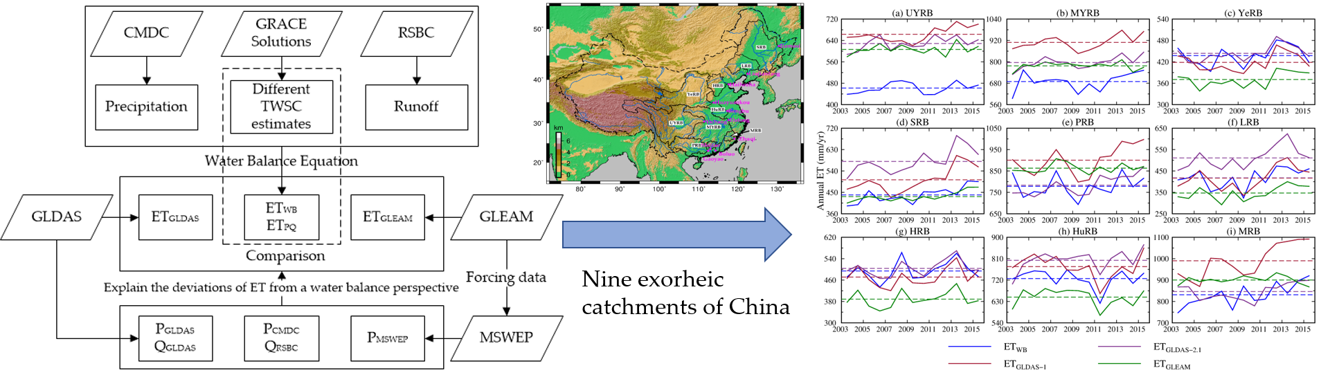
This study aims to (1) estimate the regional ET of nine exorheic catchments in China using the water balance equation considering TWSC; (2) analyze the impact of not considering TWSC and different TWSC products on the ET estimates; (3) explain the inconsistency between different ET products and regional ET from a water balance perspective. The flowchart of this study is shown in Figure 1.
2. Materials and Methods
2.1. Study Area
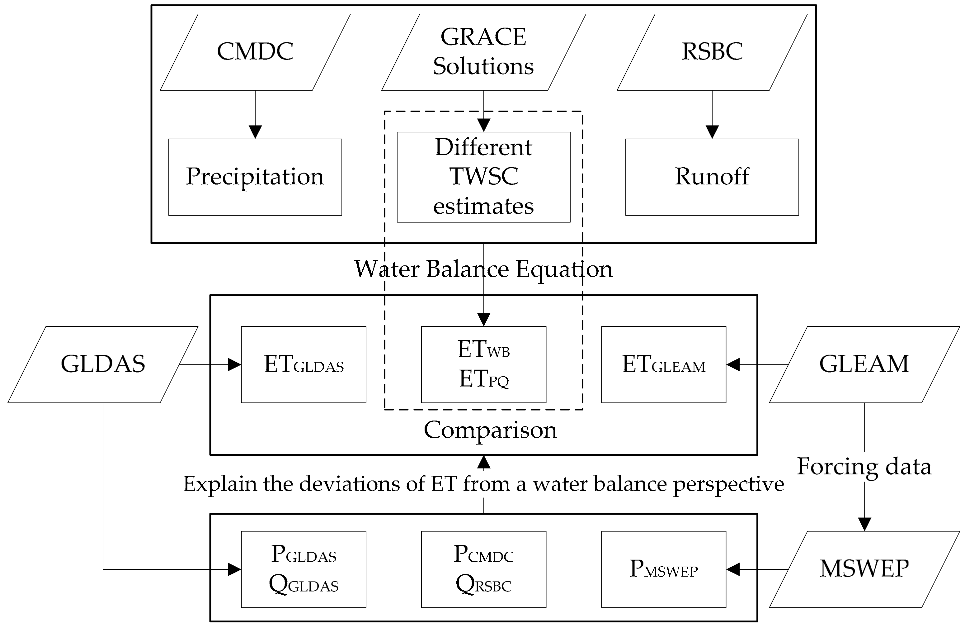
Nine exorheic catchments were divided from eleven hydrological gauge stations from River Sediment Bulletin of China (RSBC) [35]. The catchment boundaries are derived from the location of gauge stations, Shuttle Radar Topography Mission (SRTM) elevation data (https://www2.jpl.nasa.gov/srtm/), and processed in ArcGIS with Soil and Water Assessment Tool (ArcSWAT) plugin (https://swat.tamu.edu/software/arcswat/). The ArcSWAT is an ArcGIS-ArcView extension and a graphical user input interface for the SWAT (Soil and Water Assessment Tool) model. The Gaoyao, Shijiao, and Boluo hydrological gauge stations are all in the Pearl River Basin (PRB), we merge them into one catchment (Figure 2). The YRB is divided into two sub-basins, based on its two hydrological gauge stations: Yichang and Datong. The information of the nine catchments is listed in Table 1, and the catchments are also presented in Figure 2.
2.2. Water Balance Equation
The ET can be estimated from surface water balance on the basin or continental scales, which usually serves as a benchmark for other products. The equation is as follows:
where ETWB is calculated ET, P is precipitation, Q is river discharge, and ds/dt is the change in terrestrial water storage for a specific time period [4,11,15]. TWSC is estimated as the temporal derivative of TWSA from the GRACE products [37,38]. ET, P, and Q are the cumulated amount in a full month [4,39]. Then ds/dt (TWSC) is the differential of two consecutive months of TWSA at the beginning of a month. To obtain the time point of every beginning of a month of TWSA time series, we interpolate TWSA by an interpolation method. A similar process of calculation can be found in Li et al. [40]. Firstly, seasonal and trend signals are estimated using unweighted least squares and then interpolated for every beginning of a month. Secondly, the residuals removed by TWSA time series subtracting seasonal and trend signals are then interpolated by linear interpolation. Finally, the sum of interpolated residuals, seasonal, and trend signals are the interpolated TWSA time series.
ETWB = P − Q − ds/dt
Root mean square error (RMSE) is used to evaluate the deviation between ETWB and other types of ETs. The equation is as follows:
where N is the data length (time series), Xi is the ith estimated ET results from other methods, Yi is the ith ETWB result.
2.3. Data
An overview of the datasets can be found in Table 2. This table lists relevant information about the datasets used in this study, such as the TWSC, precipitation, runoff, ET, spatial resolution, and corresponding links of data access. A detailed description of these data is provided below.
2.3.1. GRACE–Derived TWSC Data
We used the Center for Space Research (CSR) GRACE RL05 Mascons data to estimate the TWSC. The mascon solutions are global and can be better applied to hydrology, oceanography, and the cryosphere without any post–processing and without applying any empirical scaling factors [41]. The data can be downloaded from http://www2.csr.utexas.edu/grace. The Mascons data is represented at a 0.5-degree lon-lat grid and is estimated with the same standards as the CSR RL05 spherical harmonics solutions using GRACE Level-1 observations. C20 coefficients were replaced, degree-1 coefficients (Geocenter) and glacial isostatic adjustment (GIA) corrections were applied. More details about the CSR GRACE RL05 Mascons (CSR-M) can be found in Save et al. [41]. With the development of post-processing GRACE satellite data, several GRACE solutions can be used for hydrology applications. However, different solutions would lead to different TWSC estimates.
To evaluate the impact of TWSC from different GRACE solutions on the estimate of ET, we also take JPL Mascons [42], CSR GRCTellus Land data [43], and CSR RL05 spherical harmonics solutions with the DDK4 filter applied (CSR-DDK4) [44] as a comparison. All of these above solutions are processed with the same C20 coefficients replaced, the same degree-1 coefficients, and GIA corrections.
The processing of JPL Mascons is based on external information provided by near-global geophysical models to constrain the solution. JPL Mascons use the coarse 3-degree spherical cap Mascons, and they are downscaled to 0.5° × 0.5° using downscaling factors (dsf) calculated from Community Land Model (CLM ver. 4.0) [42], the grid values of JPL Mascons are multiplied by downscaling factors (JPL-M.dsf). The CSR and JPL mascon solutions can be used directly without leakage corrections. CSR GRCTellus Land data is developed by Landerer and Swenson [43] from CSR data, and scaling factors are provided to account for the signal loss during processing related to truncation to degree and order 60 and application of a 300 km Gaussian smoothing filter. The grid values of CSR GRCTellus Land are multiplied by scaling factors (CSRT-GSH.sf). The DDK filter is proposed by Kusche et al. [44], and the DDK4 filter shows a good performance in the application of the upper Yellow River [45]. The process of CSR-DDK4 is similar to CSR GRCTellus Land data while replacing 300 km Gaussian smoothing filter and destriping filter with the DDK4 filter. There is no leakage correction applied in CSR-DDK4 in this study, as with in Yi et al. [45], and in fact, the results for CSR-DDK4 are at the same level with the other solutions.
2.3.2. In Situ Precipitation and Runoff Data
Gridded precipitation data was obtained from the China Meteorological Data Service Center (CMDC, hereafter, PCMDC). The gridded precipitation data was generated by a thin plate spline spatial interpolation of precipitation observations from 2472 weather stations. It has a monthly temporal resolution and 0.5° × 0.5° spatial resolution over all of China [46]. This data is validated by cross-validation and error analysis with gauge-based precipitation, indicating good quality. This precipitation data has been used in several studies [13,22,47]. The monthly runoff datasets are from eleven gauge stations recorded in RSBC (hereafter, QRSBC) (http://www.mwr.gov.cn/sj/tjgb/zghlnsgb/) [35], which integrates all runoff considering the upstream of the corresponding catchment. The runoff measurements are all from well-gauged rivers in China.
2.3.3. Land Evapotranspiration Products
We use two kinds of land evapotranspiration products for comparison, which included GLDAS ET and GLEAM ET (Table 2). Two versions of GLDAS LSM data are used for inter-comparison in this paper, i.e., GLDAS version 1 (GLDAS-1) and GLDAS version 2.1 (GLDAS-2.1) [9]. ET outputs from both GLDAS versions are driven by Noah LSM [48]. GLDAS-1 datasets cover the time period from 1979 to the present. GLDAS-2.1 datasets cover the period from 2000 to the present. Their temporal resolutions used here are monthly. More information and details about the GLDAS-1 and some improvements and changes about the GLDAS-2.1 are available at https://ldas.gsfc.nasa.gov/gldas/. The ET outputs from GLDAS-1 and GLDAS-2.1 are expressed as ETGLDAS–1 and ETGLDAS–2.1.
We use GLEAM v3.2a ET products (hereafter, ETGLEAM), which were published jointly by Vrije Universiteit Amsterdam, Netherlands and Ghent University, Belgium [6]. The data has a spatial resolution of 0.25° × 0.25° and daily temporal resolution. We sum them to the monthly results in this study. GLEAM uses a set of algorithms to separately estimate the different components (transpiration, bare-soil evaporation, interception loss, open-water evaporation, and sublimation) of land ET. The Priestley and Taylor equation was used in GLEAM to calculate potential evaporation based on observations of surface net radiation and near-surface air temperature. The rationale of GLEAM is to maximize the recovery of information on evaporation contained in current satellite observations of climatic and environmental variables [6].
2.3.4. Precipitation Forcing Data and Modeled Runoff Data
The precipitation forcing data from the GLDAS-1, GLDAS-2.1 (hereafter, PGLDAS–1 and PGLDAS–2.1), and the Multi-Source Weighted-Ensemble Precipitation (MSWEP, precipitation forcing data of GLEAM, hereafter, PMSWEP) datasets [49] are used to explain the difference of ET results. They are also computed as regional averages. As runoff is another critical variable in the water balance equation, we also calculate the mean runoff outputs of the nine exorheic catchments from GLDAS-1 and GLDAS-2.1 Noah LSM (hereafter, QGLDAS–1 and QGLDAS–2.1) and compare the results with those for in situ runoff.
2.4. Methods
In the above-mentioned data sets, which are provided with different spatial resolutions, are used with regional averages results, the different spatial resolutions have little impact on ET estimates. The grids in the catchments are used to extract regional averages estimates. Their results are computed on a monthly scale. The ET results are shown at monthly mean and annual scales, as the amount of annual ET, interannual changes, and mean annual cycles of ET are the main characteristics of ET. Besides, the difference between the ET estimates can be clearer at monthly mean and annual scales.
We use the TWSC from GRACE (CSR-M), PCMDC, and QRSBC to derive ETWB. To explore the impact of TWSC on ET estimate, we also estimate the ET from precipitation minus runoff directly (expressed as ETPQ) without considering TWSC. The results are shown in Section 3.1.1.
Here we compute TWSC results from different GRACE solutions to evaluate their impact on ET while keeping all other inputs (P and Q) unchanged (Section 3.1.2). The GRACE products include CSR-M, JPL-M.dsf, CSRT-GSH.sf, and CSR-DDK4. The TWSC used for ET estimates from JPL-M.dsf, CSRT-GSH.sf, and CSR-DDK4 are expressed as ETJPL–M.dsf, ETCSRT–GSH.sf, and ETCSR–DDK4, respectively. They are further discussed in Section 4.1.
We then compare the ET estimates from GLDAS and GLEAM with ETWB (Section 3.2). The discussion of RMSEs between ETWB and other ET estimates are shown in Section 4.2. We attempt to analyze the deviation of precipitation and runoff to the regional ET estimate from a water balance perspective (see Section 3.3 and Section 4.3), quantifying the deviations between PCMDC and precipitation forcing data, QRSBC, and QGLDAS estimates. Previous studies demonstrate that the TWSA (or TWSC) from GRACE and GLDAS are comparable [50,51,52]. Hence, we do not compare the TWSC component in the water balance equation.
We compute the deviations between water balance ET and other ET results, precipitation results, runoff results, and results of precipitation minus runoff (Section 3.3). We assess the impact of deviation of precipitation and runoff on the estimate of ET based on RMSE and the change of RMSE (Section 4.3). The RMSEs are calculated between annual ETWB minus annual PCMDC and other ET estimates minus their precipitation forcing data (expressed as RMSE (ET-P)) from a water balance perspective. Similarly, the RMSE (ET-Q) represents the calculated RMSEs between annual ETWB minus QRSBC and ETGLDAS minus QGLDAS, and the RMSE (ET-(P-Q)) represents the calculated RMSEs between annual ETWB subtracting the result of PCMDC minus QRSBC and annual ETGLDAS subtracting the result of PGLDAS minus QGLDAS from 2003–2015. The proportions of RMSEs changed of RMSE (ET-P), RMSE (ET-Q) and RMSE (ET-(P-Q)) relative to RMSE (ET) are further computed.
2.5. Uncertainty Estimation
The TWSC estimates used in the estimate of ETWB are from CSR-M. Hence, we only estimate the uncertainty of TWSC based on CSR-M. The uncertainty estimate followed the method used in Landerer and Swenson [43] and Scanlon et al. [53]. Details about the method can be found in the supporting information of Scanlon et al. [53]. As the TWSC is the differential of two consecutive months, the uncertainty of TWSC is of the uncertainty of TWSA. The uncertainties of monthly precipitation and runoff data collected by gauge are estimated to 10% and 5%, respectively [2,4,13]. The uncertainty of monthly ETWB is estimated by uncertainties of TWSC, precipitation, runoff based on error propagation law.
The monthly mean ET is the mean values of 13 months for the study period of 2003–2015, from the error propagation law, the uncertainty of monthly mean ET can be calculated as the uncertainty in monthly ETWB divided by . The uncertainty of annual ETWB is estimated from the uncertainty of annual P, Q, and TWSC based on error propagation law. Since the annual TWSC is estimated from the difference of the TWSA at the beginning month in one year and the next year, we estimate the uncertainty of annual TWSC equal to monthly TWSC.
3. Results
3.1. Impact of TWSC on ET Estimate
3.1.1. ET Estimated by Ignoring TWSC
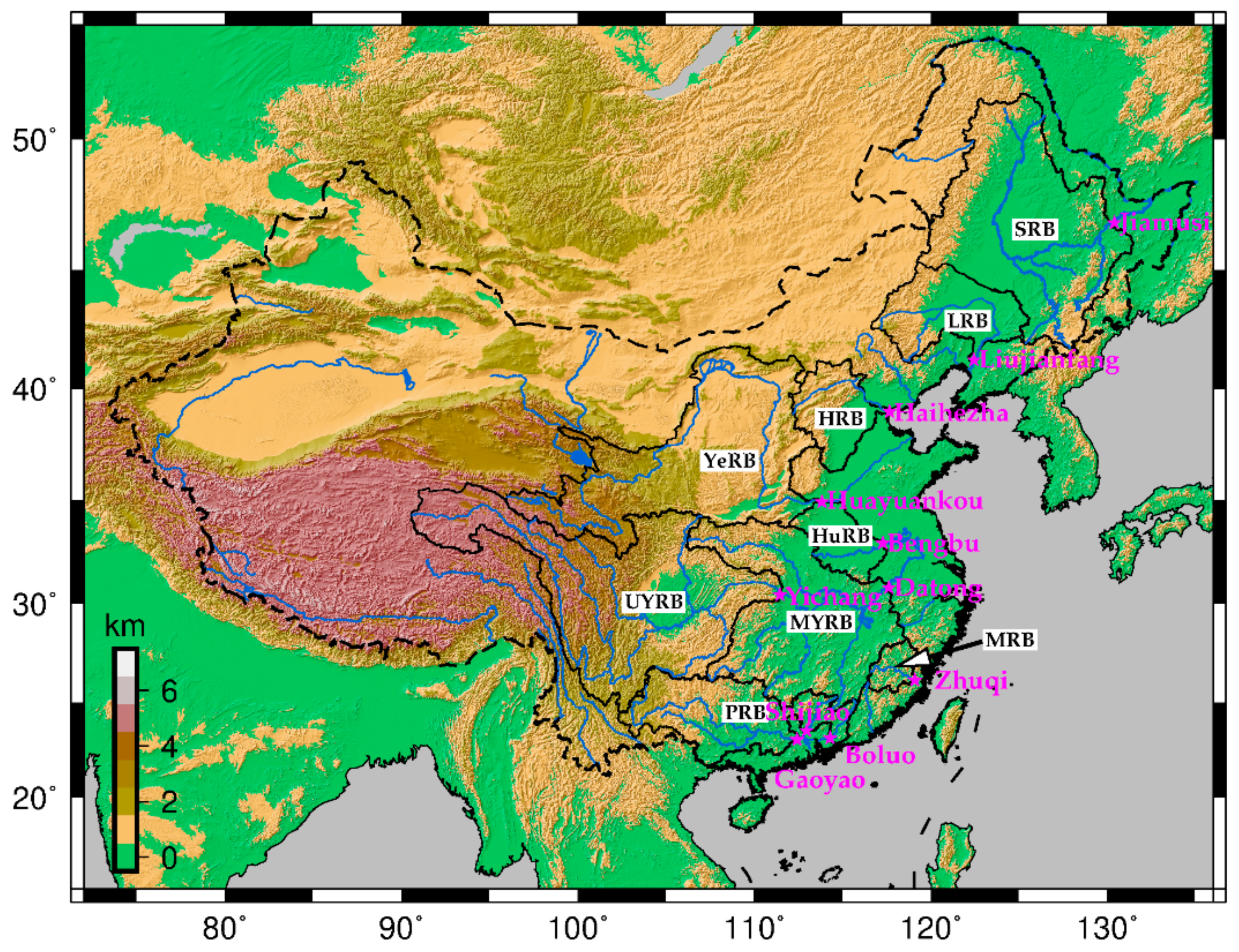
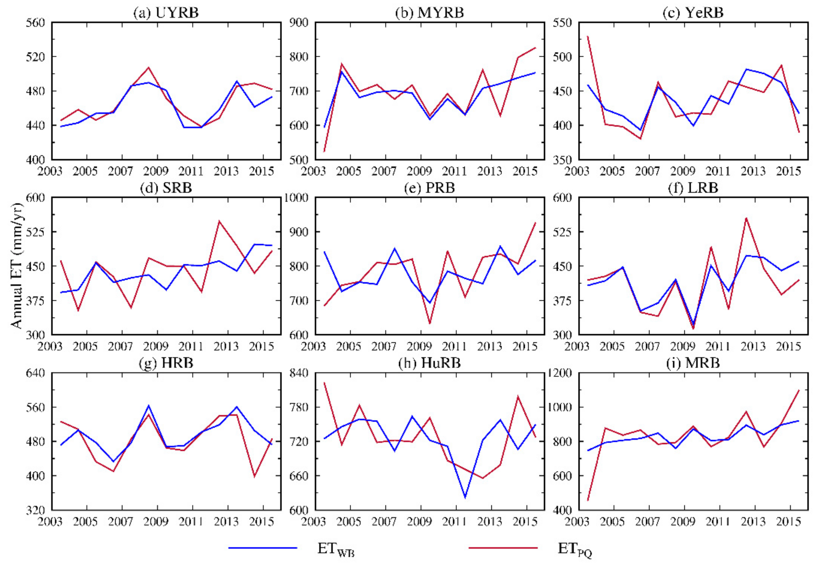
Figure 3 shows the monthly mean of ETWB following Equation 1, ETPQ, P, Q, and TWSC for 2003–2015 in the nine catchments. The negative ETWB values in January and February in the SRB and December in the Haihe River Basin (HRB) may result from the uncertainties of in situ precipitation and TWSC [13,40]. The TWSC has a significant impact on ET estimates in most catchments. The deviation of the monthly mean of ETWB and ETPQ reaches 34.2 mm/month in June (accounting for 52.9% of ETWB) in the Upper Yangtze River Basin (UYRB). The deviations between ETWB and ETPQ range from 6.7 to 37.2 mm/month for twelve months in the Middle Yangtze River Basin (MYRB), and its RMSE accounts for 37.1% of variations of ETWB. The RMSEs are computed following Equation 2. In the YeRB and SRB, the deviations between ETWB and ETPQ are small, with their RMSEs between ETWB and ETPQ reaching only 6.4 and 8.7 mm/month, respectively. In the MRB, the RMSE between ETWB and ETPQ shows the maximum value, i.e., 27.2 mm/month, accounts for 33.5% of variations of monthly mean ETWB.
The annual ETWB and ETPQ estimates are shown in Figure 4; the mean annual PCMDC, ETWB, and ETPQ results are shown in Table 3. In the UYRB, the largest deviation of annual ET between ETWB and ETPQ is only 27.5 mm/yr in 2014, and the RMSE between ETWB and ETPQ only makes up 2.6% of the mean annual ET. In the SRB, the TWSC has a large impact on annual ET, large deviations between ETWB and ETPQ occur almost all the years, and the proportion of the RMSE accounting for the mean annual ETWB reaches 11.5%. In the Minjiang River Basin (MRB), the RMSE represents 12.7% of the mean annual ET, with the largest deviation (291.8 mm/yr, 39.1% of total ETWB in this year) occurring in 2003.
3.1.2. Impact of Different GRACE Solutions on ET Estimate
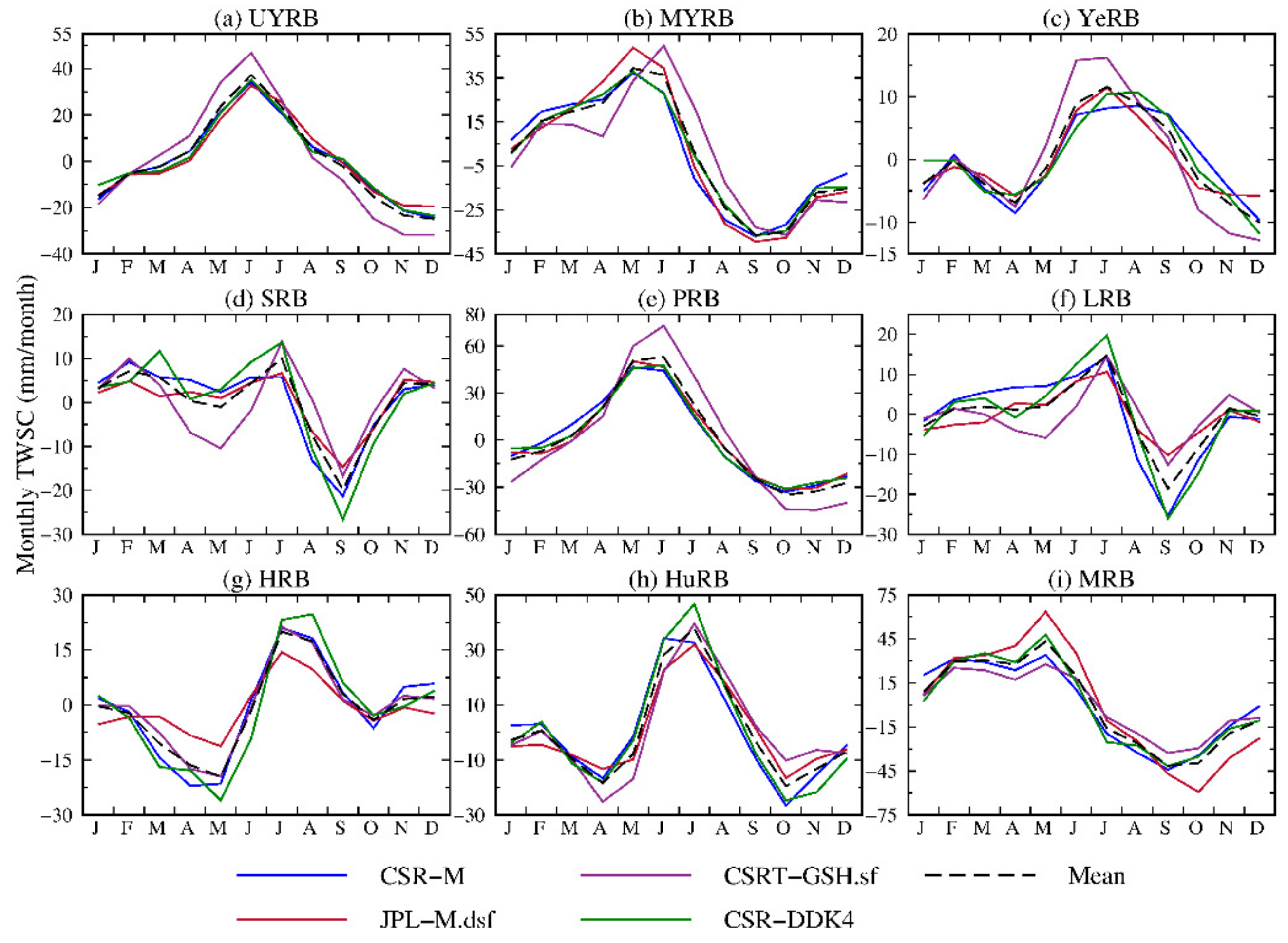
The monthly mean TWSC from different GRACE solutions is shown in Figure A1, where their mean TWSC is the arithmetical mean from all TWSC estimates for the corresponding calendar month. Note that the TWSC derived from CSR-M compare favorably with the mean TWSC (Figure A1), thus the CSR-M TWSC is used for the estimate of ETWB in this study. The TWSC from CSRT-GSH.sf show significant differences among the four TWSC results, as they exaggerate the monthly mean TWSC in the UYRB, MYRB, YeRB, SRB, and PRB, and the differences may result from the scaling factor derived from CLM4.5 [43]. The spatial distribution of scaling factors is checked in our study (not shown), and the spatial variability of scaling factors varies greatly in the basins, indicating exaggerated TWSC. The maximum deviations are calculated between each two monthly mean TWSC estimates, which range from 10.7 to 35.6 mm/month, the deviations occur in the YeRB (10.7 mm/month) and MRB (35.6 mm/month) (Figure A1c,i), respectively. As the area of MRB is the smallest, and with the most abundant precipitation, it is understandable that the MRB shows the largest deviation of TWSC. The large deviation of TWSC between JPL-M.dsf and other GRACE solutions in the HRB and MRB (Figure A1g,i) may result from the processing strategy and coarse resolution in the spatial of JPL-M since the areas of the two basins are small [54].
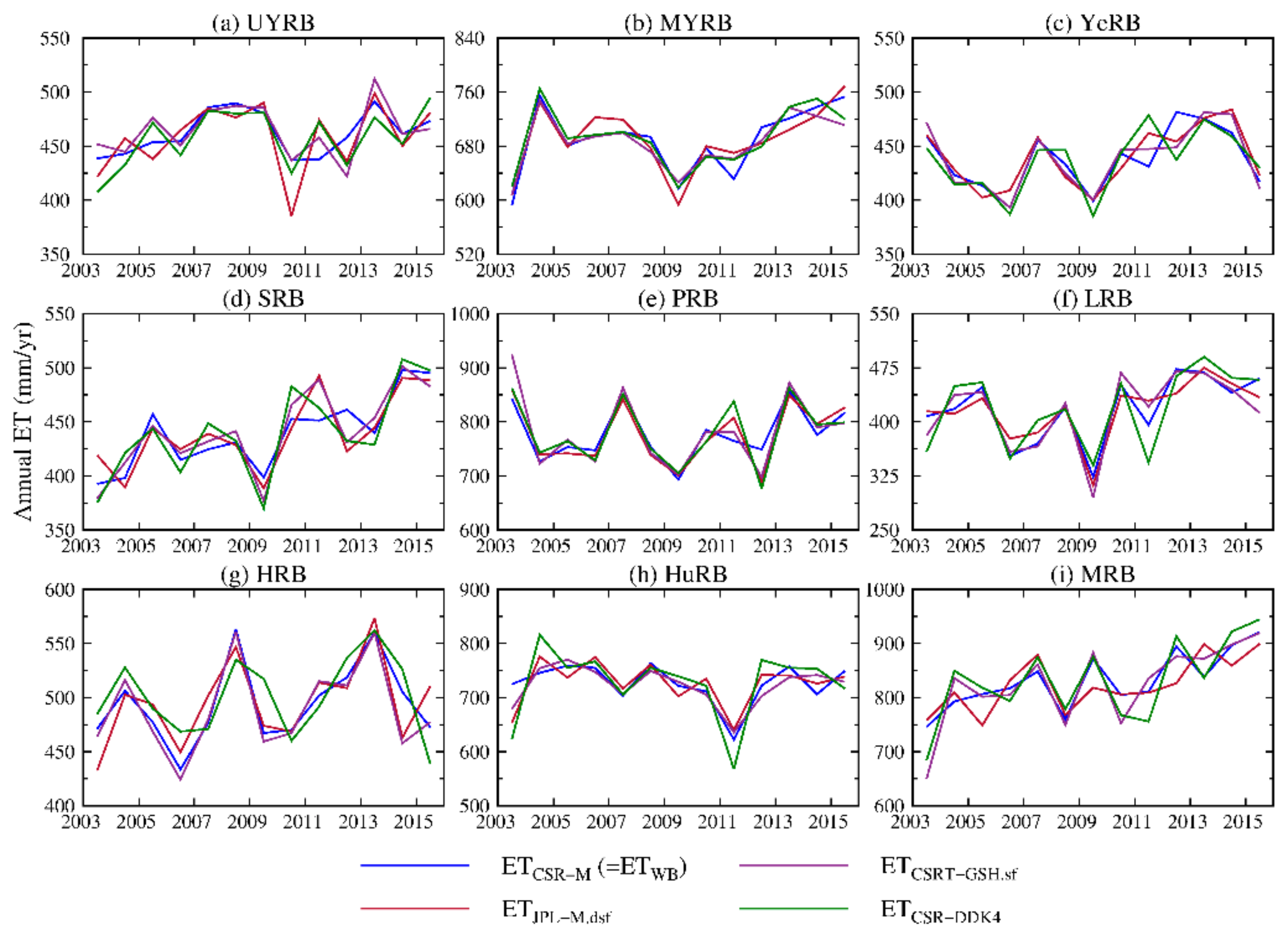
The annual ET estimates based on different GRACE solutions are shown in Figure A2. The RMSEs among ETCSR–M (=ETWB), ETJPL–M.dsf, ETCSRT–GSH.sf, and ETCSR–DDK4 are understandably less than those RMSEs between ETWB and ETPQ, and their interannual fluctuations are more consistent than that of ETPQ. We compute the standard deviations (STDs) between the four ET estimates from different GRACE solutions for every single year, and the results show that the max STD is only 51.2 mm/yr, occurring in the MRB. The mean STD for the years from 2003–2015 in the corresponding catchment is also computed, ranging from 9.7 to 27.1 mm/yr (accounting for 1.8–3.9% of annual ETWB), with the least occurring in the YeRB and the largest occurring in the MRB. In three catchments, the max STDs occur in 2003 in the PRB, the Huaihe River Basin (HuRB), and the MRB, which are located in Southeast China. In the other three catchments, the max STDs appear in 2011, which are the YeRB, SRB, and Liaohe River Basin (LRB), in North China.
3.2. Comparison of Different ET Products
Figure 5 shows the monthly mean of ET estimates from different ET products. Their mean annual cycles are similar among all the catchments. In the humid catchments: in the UYRB, the other three ET products overestimate the ET compared with ETWB for all months except December, the maximum deviation exists in July, which has the most precipitation (Figure 5a). In the MYRB, other ET estimates are bigger than ETWB estimates for all months except November when the ETWB increases to respond to increased precipitation. In the PRB, the mean of ETWB in July is less than that in June and August, and the mean of ETWB in October is also less than September and November (Figure 5e). In the HuRB, ETWB shows a rapid increase response for sharply increased precipitation in July (Figure 5h), while the three other ET results do not catch it. The ETWB also can capture the irregular monthly mean precipitation changes from June to December in the MRB (Figure 5i). In the semihumid and semiarid catchments: the two versions of GLDAS both show the maximum deviation in September with ETWB in the YeRB. Most months of ETGLDAS–2.1 are more than other ET estimates in the LRB. During the intense irrigation period of April and May, the ETWB is significantly greater than other ET estimates in the HRB. From the above, these ET results all show similar annual cycles, while ETWB can capture some irregular variations in monthly precipitation.
The maximum RMSEs between the monthly mean of ETWB and other ET results are in the MRB, which are 27.5 (vs ETGLDAS–1), 26.3 (vs ETGLDAS–2.1), and 24.7 (vs ETGLEAM) mm/month (Table A1). In the YeRB, the RMSEs are the least, which are 7.2, 7.5, and 13.0 mm/month. We also compute the proportion of the RMSEs accounting for an average of the monthly mean of ETWB. The proportions in the UYRB show the maximum values, which are 50.5% (vs ETGLDAS–1), 43.3% (vs ETGLDAS–2.1), and 43.1% (vs ETGLEAM). The HuRB experienced the minimum proportions, which are 20.4%, 22.3%, and 25.9%, respectively.
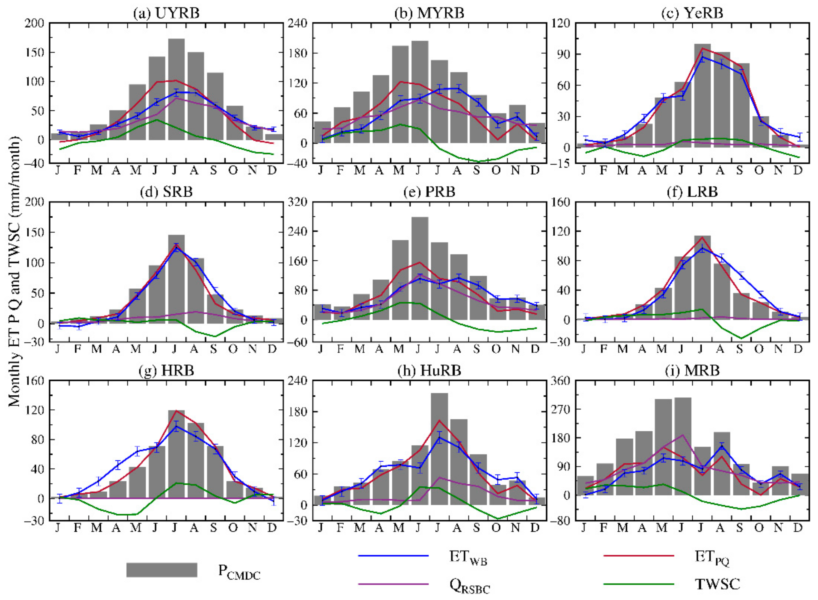
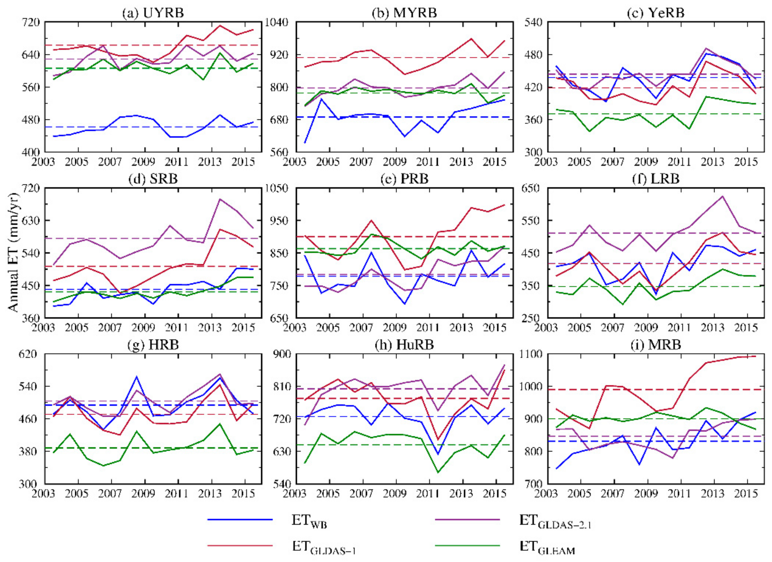
The annual ET from different sources is illustrated in Figure 6, which shows huge gaps among different ET estimates. In terms of the humid catchments: In the UYRB and MYRB, it is obvious that other annual ET estimates are all larger than ETWB. Their mean deviations between ETWB and ETGLEAM reaching 144.7 mm/yr (31.3% in mean annual ETWB) and 88.0 mm/yr (12.8% in mean annual ETWB) in the two catchments (Figure 6a,b). In the PRB, ETGLDAS–1 and ETGLEAM both overestimate the annual ET, and ETGLDAS–2.1 shows different interannual variations with respect to ETWB (Figure 6e). In the HuRB, all the ET estimates capture the drop of ET in 2011 due to reduced precipitation (Figure A3h), but there is some discrepancy among mean annual ET. In the MRB, the ET results show large differences in the interannual variations. The ETGLDAS–1 even verges on 1100 mm/yr after 2012. Concerning the semihumid and semiarid catchments: In the YeRB, the ETWB is consistent with ETGLDAS–2.1 except for the years 2006 and 2009, while ETGLEAM underestimates the annual ET for all the years. In the SRB, the ETGLDAS–2.1 is significantly greater than the other annual ET. Nevertheless, the ETGLEAM is close to ETWB. In the LRB, the ETGLDAS–1 is close to ETWB in mean annual ET, and their interannual variations are similar. In the HRB, ETGLDAS–2.1 is closest to ETWB. ETGLEAM somewhat underestimates the annual ET for the other three results. For the two catchments in Northeast China (i.e., SRB and LRB, Figure 6d,f), both ETGLDAS–2.1 results overestimate the annual ET. Additionally, the four ET results show consistent interannual changes in most catchments.
3.3. Comparison of Different Precipitation and Runoff Inputs for ET Estimation
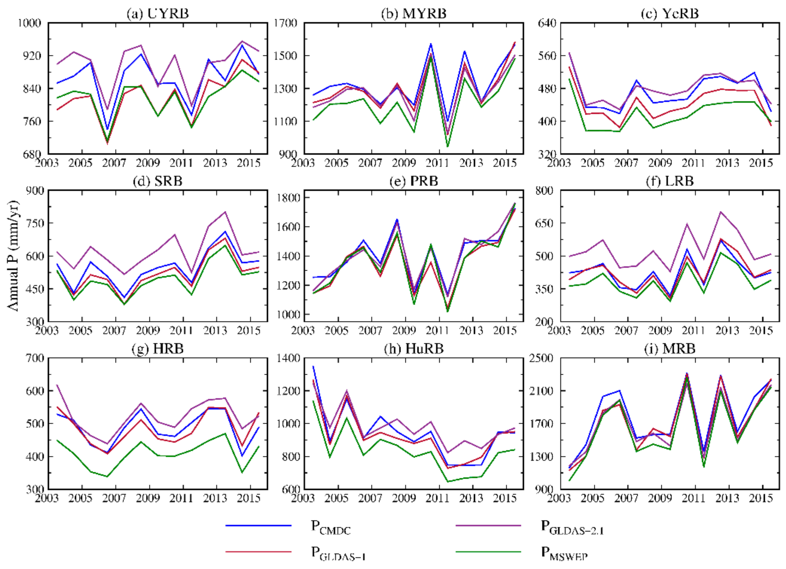
In all the catchments, the interannual fluctuations of precipitation from different sources show similar patterns (Figure A3), while the mean annual precipitation shows some differences (Figure 7). In the MYRB and YeRB, the PCMDC is higher than PGLDAS–1, which is similar to the comparison from Lv et al. [55] in corresponding regions. In the SRB and LRB (Northeast China), PGLDAS–2.1 is prominently larger than the other three precipitation sources (Figure A3d,f, and Figure 7b). Caution should be taken when using the PGLDAS–2.1 in the two catchments. It should be noted that the annual PMSWEP is the least for all the catchments (Figure A3), and mean PGLDAS–1 are all less than those of PCMDC (Figure 7a).
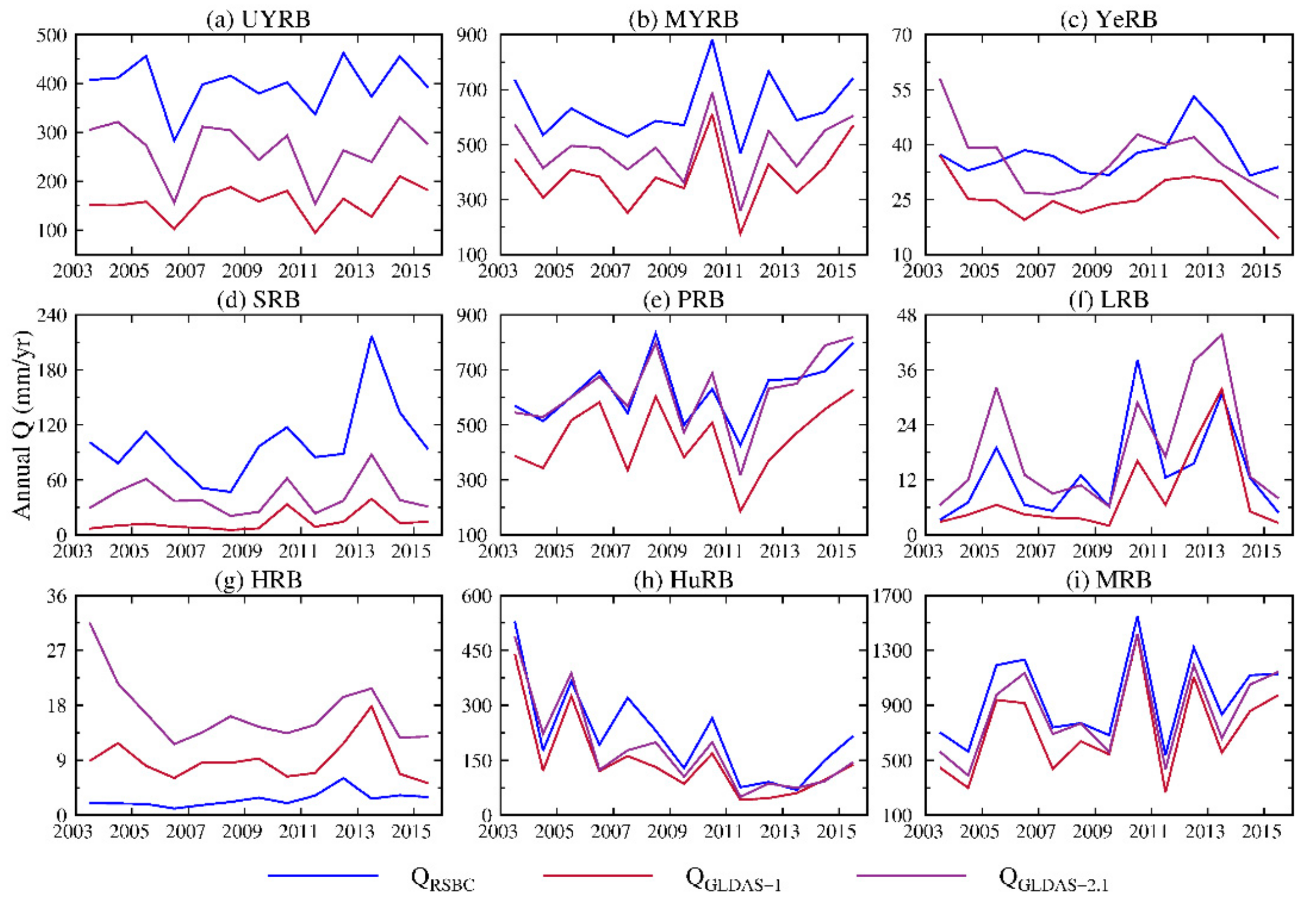
QRSBC, QGLDAS–1, and QGLDAS–2.1 show larger discrepancies than that for precipitation. The comparison of annual runoff from 2003–2015 can be found in Figure A4. Since the runoff is modeled results, it faces more uncertainties than precipitation. As the similar results showed in YRB (UYRB and MYRB) and YeRB in Lv et al. [55], the in situ runoff was significantly larger than that from QGLDAS–1. The interannual variations of runoff from different sources show similar patterns in most catchments except in the YeRB and HRB, which experienced small amounts of runoff. In all the catchments, QGLDAS–2.1 is larger than that from QGLDAS–1, and they are closer to QRSBC in most catchments, presumably due to some modification for GLDAS-2.1 [56].
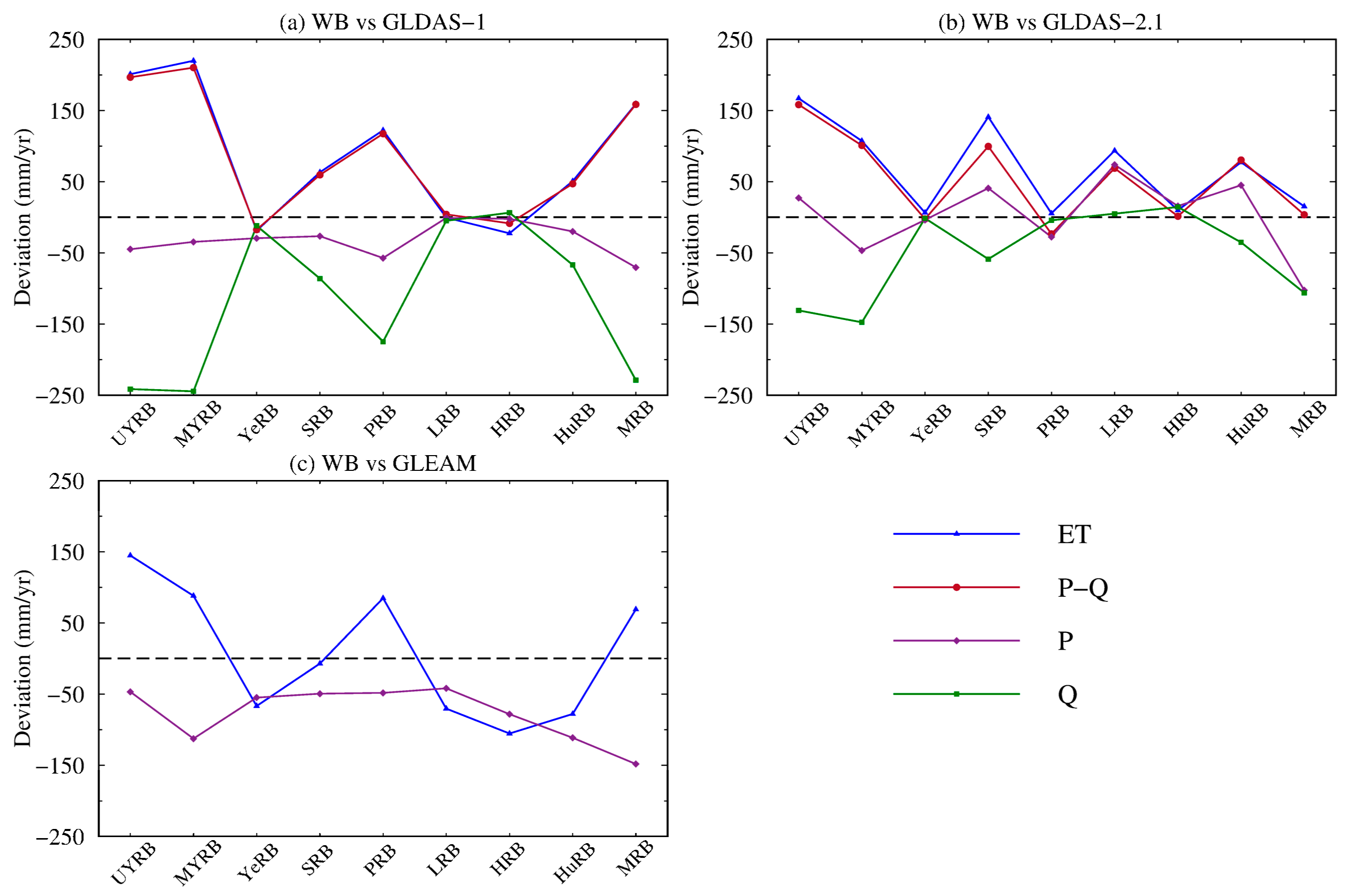
To explore the impact of precipitation and modeled runoff (GLDAS Noah LSM outputs) on ET estimates, we analyze the difference in both sides of the water balance equation. We first compute the deviation between mean annual ET, precipitation, runoff, and precipitation minus runoff for 2003–2015 (Figure 7). In the UYRB, the mean annual deviation between ETWB and ETGLDAS–1 reaches 200.9 mm/yr, the mean annual deviation between PCMDC minus QRSBC (expressed as P-Q) and PGLDAS–1 minus QGLDAS–1 are close to the deviation of ET (Figure 7a). This deviation is mostly contributed by the deviation of runoff (−241.6 mm/yr). As Figure 7a shows, the deviations of P-Q are close to the deviations of ET in all the catchments. For the water balance (WB) with GLDAS-2.1 (Figure 7b), the deviations of P-Q are close to the deviations of ET in all the catchments except PRB. In the PRB, the deviation of mean annual ET is only 5.3 mm/yr, while the deviation of mean annual precipitation reaches −27.9 mm/yr, and the deviation of mean annual runoff is −4.34 mm/yr (Figure 7b). Based on the water balance method, we only assess the precipitation forcing data variable for GLEAM ET. As Figure 7c shows, in the YeRB, LRB, and HRB, the deviation of precipitation may explain the most differences between annual ETWB and ETGLEAM. In other catchments, it is somewhat opposite between the deviation of annual precipitation and ET.
3.4. Uncertainty Estimation Results
Uncertainties of TWSC, PCMDC, QRSBC, and ETWB are shown in Table 4. Large uncertainties of TWSC appear in the PRB, HuRB, and MRB, which are more than 30 mm/month. The large uncertainties of TWSC may result from the small study area (HuRB and MRB) and large variations of TWSC caused by abundant precipitation (PRB and MRB). In three catchments (MYRB, PRB, and MRB), their annual precipitation is more than 1300 mm/yr, and their uncertainties of precipitation are also more than 11 mm/month. The uncertainties of runoff are similar to those of precipitation except the YeRB, LRB, and HRB, where the water use is intense and the runoff is little.
From Table 4, we can conclude that the uncertainties of monthly ET are mainly from TWSC, which is similar to the conclusions in Long et al. [1] and Pan et al. [13]. Almost in all the catchments, the uncertainties of TWSC are two times or even three times larger than the uncertainties of PCMDC, and they are also much larger than the uncertainties of QRSBC. The uncertainties of annual ET are all larger than 45 mm/yr, while the uncertainties are mainly from the uncertainties of annual precipitation.
4. Discussions
4.1. Impact of TWSC on ET Estimates in Local Catchments
As we can see, in the UYRB, MYRB, PRB, LRB, and HuRB, the ETWB is typically smaller than ETPQ in the wet season from May to July (Figure 3). Meanwhile, from September to December, the ETWB is larger than ETPQ. From the water balance equation, it is because, during the wet season, TWSA usually increases, and TWSC (ds/dt) is greater than 0 (Figure 3). In contrast, in the dry season with less precipitation, TWSA generally decreases, and TWSC (ds/dt) is smaller than 0, then ETWB is larger than ETPQ (Figure 3).
It should be noted that the impacts of TWSC on ET estimates are region–specific. On the monthly scale, ETWB is obviously larger than ETPQ from March to May in the HRB (Figure 3g), which is caused by the spring irrigation of wheat [13]. The ETWB is larger than ETPQ from March to May, which is 14.4, 22.1, and 21.5 (sum: 57.9) mm/month, respectively. This result is similar to the human-induced ET (60.0 ± 24.2 mm) estimated by Pan et al. [13] for the same months. While for the SRB and LRB, ETWB is obviously larger than ETPQ from August to October. Since the main crop is corn in this region, the water consumption of the growth period is ongoing in the corresponding period. Meanwhile, there is a significant reduction in PCMDC (−40.3 mm/month) in September relative to August (Figure 3f), which is different from the HRB. As the different water consumption in agriculture, the monthly TWSC are region-specific, then the deviations between ETWB and ETPQ are region-specific.
On the other hand, in the MYRB, PRB, and MRB, the RMSEs between the monthly mean of ETWB and ETPQ is significantly larger than those for other catchments. As Figure A2 shows, the amplitudes of monthly mean TWSC are stronger than other catchments. These catchments are all located in South China, with abundant precipitation [57]. During the rainy season, as the water is stored and TWSC is positive, the monthly ETWB is smaller than ETPQ in all the catchments. As the corresponding months of the rainy season are different with respect to different catchments, these catchments also show regional heterogeneities. However, the region-specific impacts of TWSC on ET deserves more research.
On the annual scale, the sizeable variations between annual ETWB and ETPQ can mostly be explained by large precipitation anomalies (Figure A3), such as the first year in the Figure 4c (YeRB) and 4i (MRB) and year 2012 in the Figure 4f (LRB). Their variations correspond to the lowest or highest precipitation during the whole study period in the corresponding catchment.
It is interesting that all the STDs of mean annual ETWB are less than those for ETPQ (see Table 3), indicating smaller interannual ETWB fluctuations. In the year with more precipitation, such as the years 2008 and 2014 in the UYRB, 2012 and 2013 in the SRB, based on the water balance equation, as the TWSA increases, TWSC is greater than 0, then ETWB should be less than ETPQ in the given year. On the contrary, in the years with precipitation deficit, as the TWSA usually decreases, the ETWB would be higher than ETPQ. We would deem that the TWSA plays a role as a reservoir in the terrestrial water cycle, impounding water and reducing the amount of water that returns to the atmosphere through evapotranspiration or other forms in the wet years, but discharging water in the dry years. We can conclude that estimating annual ET simply by subtracting runoff from precipitation would overestimate the interannual fluctuations of ET.
The difference between mean annual ETWB and ETPQ reflects the long-term rate of TWSA in a catchment. The ETWB is significantly higher than ETPQ in the HRB, where the water depletion (mainly from groundwater) is fast [58]. In the LRB and YeRB, the mean annual ETWB is also larger than ETPQ, which also indicates the water depletion there [58]. Conversely, TWSA increases in the UYRB, MYRB, SRB, and PRB, and therefore the mean annual ETWB is typically less than that for ETPQ.
4.2. The Differences between ETWB and other ET Estimates
On the monthly scale, the RMSEs between ETWB and ET from different GRACE solutions are smaller, and the ETCSR–DDK4 is closest to ETWB among the three GRACE solutions (Table A1). In the YeRB, SRB, and LRB, the maximum RMSEs are between ETWB and ETGLEAM, and all of these catchments are located in North China and are semiarid catchments. In the UYRB and MRB, the RMSEs between ETWB and ETGLDAS–1 show the maximum values. In the MYRB, PRB, HRB, and HuRB, the RMSEs between ETWB and ETPQ show the maximum values, which indicates that impacts of ignoring TWSC on the ET estimate is the most, and it should be noted that all of these catchments are humid catchments except HRB with intense water consumption.
On the annual scale, the RMSEs between ETWB and ET from the three GRACE solutions show small values, while ETCSRT–GSH.sf is closest to ETWB among the three solutions (Table A2). It indicates some differences in the TWSC estimate on the monthly and annual scales. The RMSEs between ETWB and ET from other products markedly exceed those between ETWB and ET from other GRACE solutions. In the UYRB, MYRB, PRB, and MRB, the RMSEs between ETWB and ETGLDAS–1 show the maximum values, which are all in humid regions. It should be noted that in the UYRB, the RMSE between ETWB and ETPQ is even less than the RMSEs between ETWB and ET from other GRACE solutions, which indicates that the interannual variations of TWSC are very small in this catchment. ET estimates from different GRACE solutions generally show relatively small deviations in all the catchments, and ET estimates from different products are generally relatively large deviations in the humid catchments.
4.3. Impact of Precipitation and Modeled Runoff from a Water Balance Perspective
The RMSEs between annual ETWB and other ET results are further analyzed. Their results are shown in Table A3 (WB – GLDAS-1), Table A4 (WB – GLDAS-2.1), and Table A5 (WB – GLEAM). For Table A3, in the UYRB, MYRB, SRB, PRB, and MRB, the RMSEs between ETWB and ETGLDAS–1 can be markedly reduced if the deviation of PGLDAS–1 and QGLDAS–1 can both be taken into consideration. Generally speaking, though GLDAS ET outputs are not computed based on the water balance method [9,59]. If the accuracy of PGLDAS–1 and QGLDAS–1 can be improved in China, e.g., modeled QGLDAS–1 verified by in situ runoff. Then the ET estimate would also benefit from improved runoff outputs based on the water balance equation during the simulation process. In the YeRB, LRB, HRB, and HuRB, the RMSEs are also reduced, with smaller proportions reduced than above catchments. In the YeRB and LRB, if we only consider the difference of runoff, the RMSEs would even increase, and in the HRB, the RMSE is also slightly reduced. Since the outflows are much smaller in these three catchments than other catchments, the deviation of runoff is small itself (Figure 7a). Unlike the other humid catchments, in the three semiarid catchments (YeRB, LRB, and HRB), the proportions of the RMSEs of ET–P as opposed to ET are reduced, which indicates that deviations of precipitation forcing data indeed contribute to deviations of ET.
In Table A4, the RMSEs between ETWB and ETGLDAS–2.1 reduced in all the catchments except HRB when the deviations of precipitation and runoff can be considered. In the YRB (UYRB and MYRB), the RMSEs between QRSBC and QGLDAS–2.1 account for most of the deviations. In the HRB and MRB, the deviations between ETWB and ETGLDAS–2.1 do not result from the precipitation difference. It should be noted that in the LRB, if the precipitation inconsistency is considered (Figure A3f), the RMSE between ETWB and ETGLDAS–2.1 is dramatically reduced, which can explain the cause of overestimation of the annual ET for ETGLDAS–2.1. In the HRB, with the deviation of precipitation and modeled runoff considered, the proportion of the RMSE increased (Table A4). Since the HRB is heavily influenced by human activities [13,31], the RMSE between mean annual ETWB and GLDAS ET outputs is mainly contributed by anthropogenic activities [13].
As for the RMSEs between ETWB and ETGLEAM, we only compute their precipitation difference (Table A5). In the YeRB, LRB, HRB, and HuRB, if the precipitation difference can be taken into consideration, the RMSEs between ETWB and ETGLEAM would be reduced, the YeRB, LRB, and HRB are semiarid catchments. Figure A3 also shows a large deviation between PCMDC and PMSWEP. The proportion of the RMSE reduced in the YeRB reaches 72.8%. In the UYRB, MYRB, SRB, PRB, and MRB, the RMSEs would even increase, which indicates that the deviations of precipitation do not contribute or contribute little to the deviation between ETGLEAM and ETWB. The RMSE between ET and ET–P rapidly increases from 86.9 to 228.7 mm/yr in the MRB, there is a small difference between their annual precipitation actually (Figure A3i).
Here we try to explore the deviation between ETWB and GLDAS or GLEAM ET based on the water balance equation. The RMSE (ET) would decrease if the deviation of PGLDAS and modeled QGLDAS in the GLDAS LSM can be taken into consideration. In four catchments (YeRB, LRB, HRB, and HuRB), precipitation differences contribute to the deviation between ETWB and ETGLEAM. However, the increased RMSE (ET-P), RMSE (ET-Q) and RMSE (ET-(P-Q)) relative to RMSE (ET) should be further explored. We do not investigate other forcing variables except precipitation to derive ET, e.g., radiation, air temperature, and snow water equivalent [6,9,60]. Therefore, a future intercomparison can be performed to identify the impact of these variables on ET estimates.
4.4. Impact of Groundwater Baseflow and Water Diversion on ET Estimates
Based on the water balance equation, the groundwater inflow and outflow across the basin boundary would also affect the estimate of ET. As an example, in the LRB, according to the estimate of groundwater outflow from Zhang and Li [61], the outflow is 0.61 × 10⁸ m3/yr, and its impact on the annual ET is only ~0.3 mm/yr. Therefore, it can be negligible relative to the annual ET (417.7 ± 46.5 mm/yr).
Water diversion in the basin inside and outside is also a part of basin water balance. In China, there is South-to-North water diversion, which includes the east route, the middle route, and the west route projects (http://nsbd.mwr.gov.cn/). The west route project has not been built yet. The starting point of the east route is in the mainstream of Lower Yangtze River, transporting water to Shandong Province, which is not in our study area. The middle route transports water from the MYRB to the HRB, is going through the HuRB and the YeRB. It transported water to the North in October 2014 for the first time, with a water volume of 21.67 × 10⁸ m3 in the first year. The impact on the ET estimate is 3.1 mm/yr for the MYRB, which is relatively small compared to annual ET (689.7 ± 50.3 mm/yr). If the water is totally supplied to the HRB, the impact on the ET estimate will reach 15.18 mm/yr, exerting a certain influence on the ET estimate in the HRB (494.2 ± 37.2 mm/yr). If we estimate the ET after 2015 in this region, it is necessary to account for the water diversion.
4.5. Impact of Spatial Scale on ET Estimate
The area of the MRB is only 5.45 × 10⁴ km2, which is less than the typical GRACE footprint (20 × 104 km2). However, some studies have demonstrated that GRACE is capable of detecting TWSA in local regions with an area smaller than GRACE resolution if the signal amplitude is large enough [44,62,63]. As the MYRB receives the most abundant precipitation among these catchments (Table 3), TWSA should have higher SNR (Signal to Noise Ratio), and TWSC tends to have higher reliability. On the other hand, the maximum uncertainty of monthly ET estimate is indeed in the MRB, where the uncertainties of monthly TWSC, precipitation, and runoff are also large (Table 3). Thus, we recommend that caution should be exercised when using TWSA estimates in regions with a small area.
5. Conclusions
In this study, the ET was calculated based on the water balance equation in nine exorheic catchments of China. The impacts of ignoring terrestrial water storage changes and different terrestrial water storage changes from GRACE solutions on ET estimates were analyzed. The intercomparison between ETWB and ET estimates from GLEAM, and GLDAS land surface models was also conducted. The comparison was carried out on the monthly and annual scales.
We found that the impact of ignoring terrestrial water storage changes on the estimate of ET is noteworthy. The RMSEs of between monthly mean ETWB and ETPQ range from 6.4–27.2 mm/yr (17.5–45.2% in corresponding mean monthly ET). The annual RMSEs between ETWB and ETPQ in the estimate of ET range from 12.0–105.8 mm/yr (2.6–12.7% in corresponding annual ET) among these catchments. The STDs of annual ETWB for study periods are all less than those from ETPQ, which simply estimate the annual ET by subtracting runoff from precipitation would overestimate the interannual variations of ET. Thus, TWSC should not be ignored in the estimate of ET.
The ET estimates from different GRACE solutions show relatively small deviations. The RMSEs among different GRACE solutions in most catchments are less than 10 mm/month on the monthly scale and 30 mm/yr on the annual scale. In all the catchments except the HRB and MRB, CSR-GSH.sf solutions exaggerate the monthly mean TWSC, and caution should be taken when applying this solution to derive TWSC.
Different precipitation products are assessed to explain the inconsistency between different ET products and regional ET from a water balance perspective. The difference between ETWB and ET from GLDAS land surface model results can be partly explained from deviation from precipitation forcing data in several catchments, especially in the LRB. Furthermore, the ET estimates would also benefit from improved runoff outputs during the simulation process. In the three semiarid catchments and the HuRB, the RMSEs between ETWB and ETGLEAM can be reduced, provided that the difference of precipitation can be taken into consideration. However, the increased RMSEs with deviations of precipitation forcing data and modeled runoff considering in the estimate of ET deserves further exploration.
The ET estimates show some arresting interannual fluctuations, which warrants further study. In the SRB and MRB, there may exist some positive trends, which are likely resulting from increased precipitation or other effects. The trends are also worthy of further research. In summary, our study emphasizes the capability of GRACE in estimating the ET on the basin scale. The ET estimate based on water balance can be a benchmark to other ET products, which would benefit the GLDAS LSMs and remote sensing ET estimates.
Author Contributions
Conceptualization, M.Z. and Y.Z.; Data curation, Y.Z.; Funding acquisition, Y.Z., M.Z. and B.J.; Investigation, Y.Z.; Methodology, Y.Z. and Y.M.; Supervision, M.Z. and B.J.; Writing—original draft, Y.Z.; Writing—review and editing, M.Z., Y.M. and B.J. All authors have read and agreed to the published version of the manuscript.
Funding
The research is funded by the National Natural Science Foundation of China (41874091, 41774094, and 41474061); Fundamental Research Funds for the Central Universities, China University of Geosciences (Wuhan) (G1323519314); and Open Research Fund Program of State Key Laboratory of Geodesy and Earth’s Dynamics (SKLGED2019-2-5-E, SKLGED2019-3-2-E).
Acknowledgments
The authors thank Fei Li, Wei Feng, and Haoming Yan for their insightful suggestion and discussions and thank Fan Xie for her help. We thank four anonymous reviewers for their comments, which help to improve this paper.
Conflicts of Interest
The authors declare no conflict of interest.
Appendix A
Figure A1.
Monthly mean TWSC from different GRACE solutions and products in the exorheic catchments of China from 2003–2015. (a)–(i) corresponding to the nine exorheic catchments in China.
Figure A1.
Monthly mean TWSC from different GRACE solutions and products in the exorheic catchments of China from 2003–2015. (a)–(i) corresponding to the nine exorheic catchments in China.

Figure A2.
Annual ET based on different GRACE solutions and products in the exorheic catchments of China from 2003 to 2015. (a)–(i) corresponding to the nine exorheic catchments in China.
Figure A2.
Annual ET based on different GRACE solutions and products in the exorheic catchments of China from 2003 to 2015. (a)–(i) corresponding to the nine exorheic catchments in China.

Figure A3.
Annual precipitation from CMDC, and the forcing data of two versions of GLDAS and GLEAM from 2003–2015. (a)–(i) corresponding to the nine exorheic catchments in China.
Figure A3.
Annual precipitation from CMDC, and the forcing data of two versions of GLDAS and GLEAM from 2003–2015. (a)–(i) corresponding to the nine exorheic catchments in China.

Figure A4.
Annual runoff from RSBC, GLDAS–1 Noah LSM and GLDAS–2.1 Noah LSM for 2003–2015. (a)–(i) corresponding to the nine exorheic catchments in China.
Figure A4.
Annual runoff from RSBC, GLDAS–1 Noah LSM and GLDAS–2.1 Noah LSM for 2003–2015. (a)–(i) corresponding to the nine exorheic catchments in China.


Table A1.
The root mean square errors (RMSEs) between monthly mean ETWB and other ET estimations from 2003–2015 (unit: mm/month).
Table A1.
The root mean square errors (RMSEs) between monthly mean ETWB and other ET estimations from 2003–2015 (unit: mm/month).
| Name | RMSEs between ETWB and other ET Results | ||||||
|---|---|---|---|---|---|---|---|
| ETPQ | ETJPL–M.dsf | ETCSRT–GSH.sf | ETCSR–DDK4 | ETGLDAS–1 | ETGLDAS–2.1 | ETGLEAM | |
| UYRB | 17.4 | 3.1 | 8.3 | 2.3 | 19.5 | 16.7 | 16.6 |
| MYRB | 24.9 | 6.9 | 14.8 | 4.8 | 21.4 | 13.2 | 13.8 |
| YeRB | 6.4 | 3.0 | 5.2 | 2.3 | 7.2 | 7.5 | 13.0 |
| SRB | 8.7 | 3.5 | 7.5 | 4.1 | 9.0 | 14 | 16.5 |
| PRB | 26.4 | 4.7 | 16.3 | 3.3 | 15.3 | 11.5 | 17.5 |
| LRB | 10.6 | 6.4 | 8.2 | 3.9 | 7.2 | 11.1 | 14.1 |
| HRB | 13.0 | 7.6 | 3.2 | 4.6 | 8.0 | 7.7 | 12.1 |
| HuRB | 17.8 | 7.2 | 9.9 | 5.4 | 12.3 | 13.5 | 15.7 |
| MRB | 27.2 | 17.5 | 8.8 | 8.1 | 27.5 | 26.3 | 24.7 |
Table A2.
The RMSEs between annual ETWB and other ET estimations from 2003–2015 (unit: mm/yr).
| Name | RMSEs between ETWB and other ET Results | ||||||
|---|---|---|---|---|---|---|---|
| ETPQ | ETJPL–M.dsf | ETCSRT–GSH.sf | ETCSR–DDK4 | ETGLDAS–1 | ETGLDAS–2.1 | ETGLEAM | |
| UYRB | 12.0 | 21.2 | 15.0 | 18.5 | 203.5 | 169.3 | 145.9 |
| MYRB | 46.5 | 19.5 | 18.5 | 18.2 | 222.8 | 113.3 | 100.0 |
| YeRB | 29.6 | 15 | 12.5 | 19.7 | 23.9 | 17.2 | 69.8 |
| SRB | 50.5 | 19.1 | 17.7 | 18.9 | 73.4 | 146 | 19.6 |
| PRB | 71.2 | 23.9 | 29.4 | 31.9 | 131.2 | 49.1 | 95.2 |
| LRB | 35.4 | 18.9 | 20.1 | 25.6 | 31.7 | 99.8 | 76.1 |
| HRB | 37.7 | 22.5 | 15.0 | 24.0 | 35.4 | 20.5 | 106.9 |
| HuRB | 54.7 | 26.9 | 20.1 | 43.2 | 60.3 | 86.3 | 82.7 |
| MRB | 105.8 | 37.2 | 35.5 | 33.7 | 168.4 | 52.9 | 86.9 |
Table A3.
The RMSEs between mean annual ETWB and ETGLDAS–1 (expressed as RMSE(ET)). The RMSEs between annual ETWB minus PCMDC and annual ETGLDAS–1 minus PGLDAS–1 (expressed as RMSE(ET–P)). The RMSEs between annual ETWB minus QRSBC and annual ETGLDAS–1 minus QGLDAS–1 (expressed as RMSE(ET–Q)). The RMSEs between annual ETWB subtracting the result of PCMDC minus QRSBC and annual ETGLDAS–1 subtracting the result of PGLDAS–1 minus QGLDAS–1 from 2003–2015 (expressed as RMSE(ET–(P–Q))). The proportion of RMSE changed of RMSE(ET–P) as opposed to RMSE (ET), RMSE(ET–Q) as opposed to RMSE (ET) and RMSE(ET–(P–Q)) as opposed to RMSE (ET).
| Name | RMSE (mm/yr) | Proportion of RMSE Changed (%) | |||||
|---|---|---|---|---|---|---|---|
| ET | ET-P | ET-Q | ET-(P-Q) | ET-P | ET-Q | ET-(P-Q) | |
| UYRB | 203.5 | 247.3 | 55.6 | 22.0 | 21.5 | −72.7 | −89.2 |
| MYRB | 222.8 | 258.4 | 51.6 | 31.7 | 16 | −76.8 | −85.8 |
| YeRB | 23.9 | 17.0 | 34.2 | 13.1 | −29 | 43 | −45 |
| SRB | 73.4 | 98.1 | 28.5 | 13.1 | 33.6 | −61.2 | −82.2 |
| PRB | 131.2 | 188.7 | 79.0 | 33.8 | 43.9 | −39.8 | −74.3 |
| LRB | 31.7 | 18.2 | 36.3 | 22.2 | −42.6 | 14.6 | −30.1 |
| HRB | 35.4 | 30.8 | 32.0 | 27.9 | −12.9 | −9.5 | −21.2 |
| HuRB | 60.3 | 91.3 | 37.9 | 32.8 | 51.4 | −37.2 | −45.6 |
| MRB | 168.4 | 244.3 | 100.2 | 35.1 | 45.1 | −40.5 | −79.1 |
Table A4.
The RMSEs between mean annual ETWB and ETGLDAS–2.1 (expressed as RMSE(ET)). The RMSEs between annual ETWB minus PCMDC and annual ETGLDAS–2.1 minus PGLDAS–2.1 (expressed as RMSE(ET–P)). The RMSEs between annual ETWB minus QRSBC and annual ETGLDAS–2.1 minus QGLDAS–2.1 (expressed as RMSE(ET–Q)). The RMSEs between annual ETWB subtracting the result of PCMDC minus QRSBC and annual ETGLDAS–2.1 subtracting the result of PGLDAS–2.1 minus QGLDAS–2.1 from 2003–2015 (expressed as RMSE(ET–(P–Q))). The proportion of RMSE changed of RMSE(ET–P) as opposed to RMSE (ET), RMSE(ET–Q) as opposed to RMSE (ET) and RMSE(ET–(P–Q)) as opposed to RMSE (ET).
| Name | RMSE (mm/yr) | Proportion of RMSE Changed (%) | |||||
|---|---|---|---|---|---|---|---|
| ET | ET-P | ET-Q | ET-(P-Q) | ET-P | ET-Q | ET-(P-Q) | |
| UYRB | 169.3 | 139.8 | 45.9 | 15.1 | −17.5 | −72.9 | −91.1 |
| MYRB | 113.3 | 165.8 | 59.4 | 32.7 | 46.4 | −47.6 | −71.1 |
| YeRB | 17.2 | 14.9 | 16.4 | 14.4 | −13.6 | −4.4 | −16.3 |
| SRB | 146.0 | 76.3 | 86.3 | 22.9 | −47.7 | −40.9 | −84.3 |
| PRB | 49.1 | 37.7 | 61.9 | 35.2 | −23.4 | 25.9 | −28.3 |
| LRB | 99.8 | 28.0 | 105.6 | 28.9 | −71.9 | 5.8 | −71 |
| HRB | 20.5 | 38.0 | 30.8 | 30.1 | 84.9 | 50.2 | 46.4 |
| HuRB | 86.3 | 75.3 | 64.3 | 33.3 | −12.7 | −25.5 | −61.4 |
| MRB | 52.9 | 120.7 | 117.5 | 36.9 | 128.1 | 122.1 | −30.2 |
Table A5.
The RMSEs between mean annual ETWB and ETGLEAM (expressed as RMSE(ET)), RMSEs between annual ETWB minus PCMDC and annual ETGLEAM minus PMSWEP from 2003–2015 (expressed as RMSE(ET–P)).
Table A5.
The RMSEs between mean annual ETWB and ETGLEAM (expressed as RMSE(ET)), RMSEs between annual ETWB minus PCMDC and annual ETGLEAM minus PMSWEP from 2003–2015 (expressed as RMSE(ET–P)).
| Name | RMSE (mm/yr) | Proportion of RMSE Changed (%) | |
|---|---|---|---|
| ET | ET-P | ET-P | |
| UYRB | 145.9 | 192.8 | 32.1 |
| MYRB | 100.0 | 212.6 | 112.6 |
| YeRB | 69.8 | 19.0 | −72.8 |
| SRB | 19.6 | 45.2 | 130.5 |
| PRB | 95.2 | 152.5 | 60.3 |
| LRB | 76.1 | 35.2 | −53.8 |
| HRB | 106.9 | 34.3 | −67.9 |
| HuRB | 82.7 | 51.3 | −37.9 |
| MRB | 86.9 | 228.7 | 163.0 |
References
- Long, D.; Longuevergne, L.; Scanlon, B.R. Uncertainty in evapotranspiration from land surface modeling, remote sensing, and GRACE satellites. Water Resour. Res. 2014, 50, 1131–1151. [Google Scholar] [CrossRef] [Green Version]
- Wang, K.C.; Dickinson, R.E. A review of global terrestrial evapotranspiration: observation, modeling, climatology, and climatic variability. Rev. Geophys. 2012, 50. [Google Scholar] [CrossRef]
- Miralles, D.G.; van den Berg, M.J.; Gash, J.H.; Parinussa, R.M.; de Jeu, R.A.M.; Beck, H.E.; Holmes, T.R.H.; Jiménez, C.; Verhoest, N.E.C.; Dorigo, W.A.; et al. El Niño–La Niña cycle and recent trends in continental evaporation. Nat. Clim. Change 2013, 4, 122–126. [Google Scholar] [CrossRef]
- Rodell, M.; Famiglietti, J.S.; Chen, J.; Seneviratne, S.I.; Viterbo, P.; Holl, S.; Wilson, C.R. Basin scale estimates of evapotranspiration using GRACE and other observations. Geophys. Res. Lett. 2004, 31, 1–4. [Google Scholar] [CrossRef] [Green Version]
- Yu, G.R.; Wen, X.F.; Sun, X.M.; Tanner, B.D.; Lee, X.H.; Chen, J.Y. Overview of ChinaFLUX and evaluation of its eddy covariance measurement. Agric. For. Meteorol. 2006, 137, 125–137. [Google Scholar] [CrossRef]
- Martens, B.; Miralles, D.G.; Lievens, H.; van der Schalie, R.; de Jeu, R.A.M.; Fernandez–Prieto, D.; Beck, H.E.; Dorigo, W.A.; Verhoest, N.E.C. GLEAM v3: satellite–based land evaporation and root–zone soil moisture. Geosci. Model Dev. 2017, 10, 1903–1925. [Google Scholar] [CrossRef] [Green Version]
- Mu, Q.Z.; Zhao, M.S.; Running, S.W. Improvements to a MODIS global terrestrial evapotranspiration algorithm. Remote Sens. Environ. 2011, 115, 1781–1800. [Google Scholar] [CrossRef]
- Yang, Y.T.; Long, D.; Shang, S.H. Remote estimation of terrestrial evapotranspiration without using meteorological data. Geophys. Res. Lett. 2013, 40, 3026–3030. [Google Scholar] [CrossRef]
- Rodell, M.; Houser, P.R.; Jambor, U.; Gottschalck, J.; Mitchell, K.; Meng, C.J.; Arsenault, K.; Cosgrove, B.; Radakovich, J.; Bosilovich, M.; et al. The global land data assimilation system. Bull. Am. Meteorol. Soc. 2004, 85, 381–394. [Google Scholar] [CrossRef] [Green Version]
- Bai, P.; Liu, X.M. Intercomparison and evaluation of three global high–resolution evapotranspiration products across China. J. Hydrol. 2018, 566, 743–755. [Google Scholar] [CrossRef]
- Liu, W.B.; Wang, L.; Zhou, J.; Li, Y.Z.; Sun, F.B.; Fu, G.B.; Li, X.P.; Sang, Y.F. A worldwide evaluation of basin–scale evapotranspiration estimates against the water balance method. J. Hydrol. 2016, 538, 82–95. [Google Scholar] [CrossRef] [Green Version]
- Tapley, B.D.; Bettadpur, S.; Ries, J.C.; Thompson, P.F.; Watkins, M.M. GRACE measurements of mass variability in the Earth system. Science 2004, 305, 503–505. [Google Scholar] [CrossRef] [PubMed] [Green Version]
- Pan, Y.; Zhang, C.; Gong, H.L.; Yeh, P.J.F.; Shen, Y.J.; Guo, Y.; Huang, Z.Y.; Li, X.J. Detection of human–induced evapotranspiration using GRACE satellite observations in the Haihe River basin of China. Geophys. Res. Lett. 2017, 44, 190–199. [Google Scholar] [CrossRef]
- Eicker, A.; Forootan, E.; Springer, A.; Longuevergne, L.; Kusche, J. Does GRACE see the terrestrial water cycle “intensifying”? J. Geophys. Res. Atmos. 2016, 121, 733–745. [Google Scholar] [CrossRef] [Green Version]
- Ramillien, G.; Frappart, F.; Guntner, A.; Ngo–Duc, T.; Cazenave, A.; Laval, K. Time variations of the regional evapotranspiration rate from Gravity Recovery and Climate Experiment (GRACE) satellite gravimetry. Water Resour. Res. 2006, 42, 1–8. [Google Scholar] [CrossRef] [Green Version]
- Boronina, A.; Ramillien, G. Application of AVHRR imagery and GRACE measurements for calculation of actual evapotranspiration over the Quaternary aquifer (Lake Chad basin) and validation of groundwater models. J. Hydrol. 2008, 348, 98–109. [Google Scholar] [CrossRef]
- Ferguson, C.R.; Sheffield, J.; Wood, E.F.; Gao, H.L. Quantifying uncertainty in a remote sensing–based estimate of evapotranspiration over continental USA. Int. J. Remote Sens. 2010, 31, 3821–3865. [Google Scholar] [CrossRef]
- Swann, A.L.S.; Koven, C.D. A Direct Estimate of the Seasonal Cycle of Evapotranspiration over the Amazon Basin. J. Hydrometeorol. 2017, 18, 2173–2185. [Google Scholar] [CrossRef] [Green Version]
- Castle, S.L.; Reager, J.T.; Thomas, B.F.; Purdy, A.J.; Lo, M.H.; Famiglietti, J.S.; Tang, Q.H. Remote detection of water management impacts on evapotranspiration in the Colorado River Basin. Geophys. Res. Lett. 2016, 43, 5089–5097. [Google Scholar] [CrossRef] [Green Version]
- Dee, D.P.; Uppala, S.M.; Simmons, A.J.; Berrisford, P.; Poli, P.; Kobayashi, S.; Andrae, U.; Balmaseda, M.A.; Balsamo, G.; Bauer, P. The ERA–Interim reanalysis: configuration and performance of the data assimilation system. Q. J. R. Meteorolog. Soc. 2011, 137, 553–597. [Google Scholar] [CrossRef]
- Badgley, G.; Fisher, J.B.; Jimenez, C.; Tu, K.P.; Vinukollu, R. On Uncertainty in Global Terrestrial Evapotranspiration Estimates from Choice of Input Forcing Datasets. J. Hydrometeorol. 2015, 16, 1449–1455. [Google Scholar] [CrossRef]
- Mao, Y.N.; Wang, K.C.; Liu, X.M.; Liu, C.M. Water storage in reservoirs built from 1997 to 2014 significantly altered the calculated evapotranspiration trends over China. J. Geophys. Res. Atmos. 2016, 121, 10097–10112. [Google Scholar] [CrossRef]
- Mao, Y.N.; Wang, K.C. Comparison of evapotranspiration estimates based on the surface water balance, modified Penman–Monteith model, and reanalysis data sets for continental China. J. Geophys. Res. Atmos. 2017, 122, 3228–3244. [Google Scholar] [CrossRef]
- Jiang, Y.Y.; Wang, W.; Zhou, Z.H. Evaluation of MODIS MOD16 Evapotranspiration Product in Chinese River Basins. J. Nat. Resour. 2017, 32, 517–528. [Google Scholar] [CrossRef]
- Li, X.L.; Liang, S.L.; Yuan, W.P.; Yu, G.R.; Cheng, X.; Chen, Y.; Zhao, T.B.; Feng, J.M.; Ma, Z.G.; Ma, M.G.; et al. Estimation of evapotranspiration over the terrestrial ecosystems in China. Ecohydrology 2014, 7, 139–149. [Google Scholar] [CrossRef]
- Mu, Q.Z.; Heinsch, F.A.; Zhao, M.; Running, S.W. Development of a global evapotranspiration algorithm based on MODIS and global meteorology data. Remote Sens. Environ. 2007, 111, 519–536. [Google Scholar] [CrossRef]
- Cleugh, H.A.; Leuning, R.; Mu, Q.Z.; Running, S.W. Regional evaporation estimates from flux tower and MODIS satellite data. Remote Sens. Environ. 2007, 106, 285–304. [Google Scholar] [CrossRef]
- Zhang, Y.Q.; Leuning, R.; Chiew, F.H.S.; Wang, E.L.; Zhang, L.; Liu, C.M.; Sun, F.B.; Peel, M.C.; Shen, Y.J.; Jung, M. Decadal Trends in Evaporation from Global Energy and Water Balances. J. Hydrometeorol. 2012, 13, 379–391. [Google Scholar] [CrossRef]
- Senay, G.B.; Leake, S.; Nagler, P.L.; Artan, G.; Dickinson, J.; Cordova, J.T.; Glenn, E.P. Estimating basin scale evapotranspiration (ET) by water balance and remote sensing methods. Hydrol. Process. 2011, 25, 4037–4049. [Google Scholar] [CrossRef]
- Xue, B.L.; Wang, L.; Li, X.P.; Yang, K.; Chen, D.L.; Sun, L.T. Evaluation of evapotranspiration estimates for two river basins on the Tibetan Plateau by a water balance method. J. Hydrol. 2013, 492, 290–297. [Google Scholar] [CrossRef]
- Feng, W.; Zhong, M.; Lemoine, J.M.; Biancale, R.; Hsu, H.T.; Xia, J. Evaluation of groundwater depletion in North China using the Gravity Recovery and Climate Experiment (GRACE) data and ground–based measurements. Water Resour. Res. 2013, 49, 2110–2118. [Google Scholar] [CrossRef]
- Scanlon, B.R.; Longuevergne, L.; Long, D. Ground referencing GRACE satellite estimates of groundwater storage changes in the California Central Valley, USA. Water Resour. Res. 2012, 48. [Google Scholar] [CrossRef] [Green Version]
- Zeng, Z.Z.; Piao, S.L.; Lin, X.; Yin, G.D.; Peng, S.S.; Ciais, P.; Myneni, R.B. Global evapotranspiration over the past three decades: estimation based on the water balance equation combined with empirical models. Environ. Res. Lett. 2012, 7, 014026. [Google Scholar] [CrossRef]
- Wang, D.B. Evaluating interannual water storage changes at watersheds in Illinois based on long–term soil moisture and groundwater level data. Water Resour. Res. 2012, 48. [Google Scholar] [CrossRef]
- Ministry of Water Resources of the People’s Republic of China (MWR). River Sediment Bulletin of China; Ministry of Water Resour. of the PRC, Ed.; China Water Power Press: Beijing, China, 2013; p. 85.
- Tan, Y.J. Alternation of Dry and Wet Climate Zone and its Cause Analysis in China in Last 50 Years; Nanjing University of Information Technology: Nanjing, China, 2016. [Google Scholar]
- Forootan, E.; Safari, A.; Mostafaie, A.; Schumacher, M.; Delavar, M.; Awange, J.L. Large–Scale Total Water Storage and Water Flux Changes over the Arid and Semiarid Parts of the Middle East from GRACE and Reanalysis Products. Surv. Geophys. 2016, 38, 591–615. [Google Scholar] [CrossRef] [Green Version]
- Long, D.; Shen, Y.J.; Sun, A.; Hong, Y.; Longuevergne, L.; Yang, Y.T.; Li, B.; Chen, L. Drought and flood monitoring for a large karst plateau in Southwest China using extended GRACE data. Remote Sens. Environ. 2014, 155, 145–160. [Google Scholar] [CrossRef]
- Li, Q.; Luo, Z.C.; Zhong, B.; Zhou, H. An Improved Approach for Evapotranspiration Estimation Using Water Balance Equation: Case Study of Yangtze River Basin. Water 2018, 10, 812. [Google Scholar] [CrossRef] [Green Version]
- Li, X.Y.; Long, D.; Han, Z.Y.; Scanlon, B.R.; Sun, Z.L.; Han, P.F.; Hou, A.Z. Evapotranspiration Estimation for Tibetan Plateau Headwaters Using Conjoint Terrestrial and Atmospheric Water Balances and Multisource Remote Sensing. Water Resour. Res. 2019, 55, 8608–8630. [Google Scholar] [CrossRef]
- Save, H.; Bettadpur, S.; Tapley, B.D. High–resolution CSR GRACE RL05 mascons. J. Geophys. Res. Solid Earth 2016, 121, 7547–7569. [Google Scholar] [CrossRef]
- Wiese, D.N.; Landerer, F.W.; Watkins, M.M. Quantifying and reducing leakage errors in the JPL RL05M GRACE mascon solution. Water Resour. Res. 2016, 52, 7490–7502. [Google Scholar] [CrossRef]
- Landerer, F.W.; Swenson, S.C. Accuracy of scaled GRACE terrestrial water storage estimates. Water Resour. Res. 2012, 48. [Google Scholar] [CrossRef]
- Kusche, J.; Schmidt, R.; Petrovic, S.; Rietbroek, R. Decorrelated GRACE time–variable gravity solutions by GFZ, and their validation using a hydrological model. J. Geod. 2009, 83, 903–913. [Google Scholar] [CrossRef] [Green Version]
- Yi, S.; Song, C.Q.; Wang, Q.Y.; Wang, L.S.; Heki, K.; Sun, W.K. The potential of GRACE gravimetry to detect the heavy rainfall–induced impoundment of a small reservoir in the upper Yellow River. Water Resour. Res. 2017, 53, 6562–6578. [Google Scholar] [CrossRef]
- Zhao, Y.; Zhu, J.; Xu, Y. Establishment and assessment of the grid precipitation datasets in China for recent 50 years. J. Meteorol. Sci 2014, 34, 414–420. [Google Scholar] [CrossRef]
- Ren, Z.G.; Zhang, M.J.; Wang, S.J.; Qiang, F.; Zhu, X.F.; Dong, L. Changes in daily extreme precipitation events in South China from 1961 to 2011. J. Geog. Sci. 2015, 25, 58–68. [Google Scholar] [CrossRef]
- Ek, M.B.; Mitchell, K.E.; Lin, Y.; Rogers, E.; Grunmann, P.; Koren, V.; Gayno, G.; Tarpley, J.D. Implementation of Noah land surface model advances in the National Centers for Environmental Prediction operational mesoscale Eta model. J. Geophys. Res. Atmos. 2003, 108. [Google Scholar] [CrossRef]
- Beck, H.E.; van Dijk, A.I.J.M.; Levizzani, V.; Schellekens, J.; Miralles, D.G.; Martens, B.; de Roo, A. MSWEP: 3–hourly 0.25 degrees global gridded precipitation (1979–2015) by merging gauge, satellite, and reanalysis data. Hydrol. Earth Syst. Sci. 2017, 21, 589–615. [Google Scholar] [CrossRef] [Green Version]
- Zhang, Z.Z.; Chao, B.F.; Chen, J.L.; Wilson, C.R. Terrestrial water storage anomalies of Yangtze River Basin droughts observed by GRACE and connections with ENSO. Global Planet. Change 2015, 126, 35–45. [Google Scholar] [CrossRef]
- Zhong, Y.L.; Zhong, M.; Feng, W.; Zhang, Z.Z.; Shen, Y.C.; Wu, D.C. Groundwater Depletion in the West Liaohe River Basin, China and Its Implications Revealed by GRACE and In Situ Measurements. Remote Sens. 2018, 10, 493. [Google Scholar] [CrossRef] [Green Version]
- Syed, T.H.; Famiglietti, J.S.; Rodell, M.; Chen, J.; Wilson, C.R. Analysis of terrestrial water storage changes from GRACE and GLDAS. Water Resour. Res. 2008, 44. [Google Scholar] [CrossRef]
- Scanlon, B.R.; Zhang, Z.Z.; Save, H.; Wiese, D.N.; Landerer, F.W.; Long, D.; Longuevergne, L.; Chen, J.L. Global evaluation of new GRACE mascon products for hydrologic applications. Water Resour. Res. 2016, 52, 9412–9429. [Google Scholar] [CrossRef]
- Ran, J.; Ditmar, P.; Klees, R.; Farahani, H.H. Statistically optimal estimation of Greenland Ice Sheet mass variations from GRACE monthly solutions using an improved mascon approach. J. Geod. 2018, 92, 299–319. [Google Scholar] [CrossRef] [PubMed] [Green Version]
- Lv, M.X.; Ma, Z.G.; Yuan, X.; Lv, M.Z.; Li, M.X.; Zheng, Z.Y. Water budget closure based on GRACE measurements and reconstructed evapotranspiration using GLDAS and water use data for two large densely–populated mid–latitude basins. J. Hydrol. 2017, 547, 585–599. [Google Scholar] [CrossRef]
- Rodell, M.; Beaudoing, H.K. GLDAS Noah Land Surface Model L4 monthly 1 x 1 degree V2.1; NASA/GSFC/HSL, Ed.; Goddard Space Flight Center Earth Sciences Data and Information Services Center (GES DISC): Greenbelt, MD, USA, 2016. [Google Scholar] [CrossRef]
- Zhang, Q.; Singh, V.P.; Sun, P.; Chen, X.; Zhang, Z.X.; Li, J.F. Precipitation and streamflow changes in China: changing patterns, causes and implications. J. Hydrol. 2011, 410, 204–216. [Google Scholar] [CrossRef]
- Feng, W.; Shum, C.K.; Zhong, M.; Pan, Y. Groundwater Storage Changes in China from Satellite Gravity: An Overview. Remote Sens. 2018, 10, 674. [Google Scholar] [CrossRef] [Green Version]
- Rui, H.; Beaudoing, H. Readme Document for Global Land Data Assimilation System Version 2 (GLDAS–2) Products; DISC/HSL Group, Ed.; Goddard Space Flight Center Earth Sciences Data and Information Services Center (GES DISC): Greenbelt, MD, USA, 2011. [Google Scholar]
- Wang, M.M.; He, G.J.; Zhang, Z.M.; Wang, G.Z.; Zhang, Z.J.; Cao, X.J.; Wu, Z.J.; Liu, X.G. Comparison of Spatial Interpolation and Regression Analysis Models for an Estimation of Monthly Near Surface Air Temperature in China. Remote Sens. 2017, 9, 1278. [Google Scholar] [CrossRef] [Green Version]
- Zhang, Z.H.; Li, L.R. Groundwater Resources of China (Liaoning Volume); China Cartographic Publishing House: Beijing, China, 2005; p. 111. [Google Scholar]
- Longuevergne, L.; Wilson, C.R.; Scanlon, B.R.; Cretaux, J.F. GRACE water storage estimates for the Middle East and other regions with significant reservoir and lake storage. Hydrol. Earth Syst. Sci. 2013, 17, 4817–4830. [Google Scholar] [CrossRef] [Green Version]
- Wang, X.W.; de Linage, C.; Famiglietti, J.; Zender, C.S. Gravity Recovery and Climate Experiment (GRACE) detection of water storage changes in the Three Gorges Reservoir of China and comparison with in situ measurements. Water Resour. Res. 2011, 47. [Google Scholar] [CrossRef]
Figure 1.
Flowchart of this study. It includes the used data and process of calculation and analysis in this study.
Figure 1.
Flowchart of this study. It includes the used data and process of calculation and analysis in this study.

Figure 2.
Map of exorheic catchments of China. The black curves show the boundaries of the nine exorheic catchments, the black texts with a white background are the abbreviation of catchments names. The magenta stars show the locations of eleven hydrological gauge stations, and the magenta texts present the name of hydrological gauge stations. Their descriptions can be further found in Table 1. The blue curves represent the main rivers and tributaries in China. The country boundary is shown with the dash line.

Figure 3.
Monthly mean of ETWB (blue curves), ETPQ (red lines), P, Q (purple lines), and TWSC (green lines) for 2003–2015 in the nine exorheic catchments. The histograms represent the monthly precipitation (P). The error bars show the uncertainties of monthly mean ETWB. (a)–(i) corresponding to the nine exorheic catchments in China. (a): UYRB; (b): MYRB; (c) YeRB; (d): SRB; (e): PRB; (f): LRB; (g) HRB; (h): HuRB; (i): MRB.

Figure 4.
Annual ETWB and ETPQ from 2003–2015. (a)–(i) corresponding to the nine exorheic catchments in China.
Figure 4.
Annual ETWB and ETPQ from 2003–2015. (a)–(i) corresponding to the nine exorheic catchments in China.

Figure 5.
Monthly mean of ET estimates in the exorheic catchments of China. The error bars show the uncertainties of monthly mean ETWB. (a)–(i) corresponding to the nine exorheic catchments in China.
Figure 5.
Monthly mean of ET estimates in the exorheic catchments of China. The error bars show the uncertainties of monthly mean ETWB. (a)–(i) corresponding to the nine exorheic catchments in China.

Figure 6.
Annual ET from different products in the exorheic catchments of China. The dotted lines with different colors corresponding to their mean annual ET. (a)–(i) corresponding to the nine exorheic catchments in China.
Figure 6.
Annual ET from different products in the exorheic catchments of China. The dotted lines with different colors corresponding to their mean annual ET. (a)–(i) corresponding to the nine exorheic catchments in China.

Figure 7.
Deviations of annual ET, precipitation, and runoff between (a): WB and GLDAS–1; (b): WB and GLDAS–2.1; (c): WB and GLEAM. The blue curves with triangles represent the deviations between annual ET and other ET estimates. The red curves with dots represent the deviations between PCMDC minus QRSBC and PGLDAS minus the QGLDAS. The purple lines with rhombus points represent the deviations between PCMDC and other precipitation forcing data. The green lines with square points represent the deviations of runoff between QRSBC and two versions of QGLDAS.

Table 1.
Descriptions for the nine exorheic catchments of China (sorted by areas and location). The climate categories are based on annual precipitation and dryness [36].
Table 1.
Descriptions for the nine exorheic catchments of China (sorted by areas and location). The climate categories are based on annual precipitation and dryness [36].
| Catchments ID | Name | Hydrological Gauge Stations | Area (× 104 km2) | Climate Categories |
|---|---|---|---|---|
| 1 | Upper Yangtze River Basin (UYRB) | Yichang | 100.55 | Humid |
| 2 | Middle Yangtze River Basin (MYRB) | Datong-Yichang | 69.99 | Humid |
| 3 | Yellow River Basin (YeRB) | Huayuankou | 73.00 | Semiarid |
| 4 | Songhuajiang River Basin (SRB) | Jiamusi | 52.83 | Semihumid |
| 5 | Pearl River Basin (PRB) | Gaoyao + Shijiao + Boluo | 41.52 | Humid |
| 6 | Liaohe River Basin (LRB) | Liujianfang | 18.58 | Semiarid |
| 7 | Haihe River Basin (HRB) | Haihezha | 14.28 | Semiarid |
| 8 | Huaihe River Basin (HuRB) | Bengbu | 12.13 | Humid |
| 9 | Minjiang River Basin (MRB) | Zhuqi | 5.45 | Humid |
Table 2.
Summary of the datasets used in this study.
| Type | Data Name | Data Version/Source | Spatial Resolution | Data Access |
|---|---|---|---|---|
| Satellite | TWSC | CSR-M | 0.5° × 0.5° | http://www2.csr.utexas.edu/grace |
| JPL-M | 0.5° × 0.5° | https://grace.jpl.nasa.gov/data/get-data/ | ||
| CSRT-GSH | 1° × 1° | https://grace.jpl.nasa.gov/data/get-data/ | ||
| CSR-DDK4 | 1° × 1° | http://icgem.gfz-potsdam.de/home | ||
| In situ | Precipitation | CMDC v2.0 | 0.5° × 0.5° | http://data.cma.cn/ |
| Runoff | RSBC | Station | http://www.mwr.gov.cn/sj/tjgb/zghlnsgb/ | |
| Model | ET | GLDAS-1 Noah | 1° × 1° | https://ldas.gsfc.nasa.gov/gldas/ |
| GLDAS-2.1 Noah | 1° × 1° | |||
| GLEAM v3.2a | 0.25° × 0.25° | https://www.gleam.eu/ | ||
| Runoff | GLDAS-1 Noah | 1° × 1° | https://ldas.gsfc.nasa.gov/gldas/ | |
| GLDAS-2.1 Noah | 1° × 1° | |||
| Forcing data | Precipitation | GLDAS-1 Noah | 1° × 1° | |
| GLDAS-2.1 Noah | 1° × 1° | |||
| MSWEP | 0.5° × 0.5° | http://www.gloh2o.org/ |
Table 3.
The mean annual precipitation from CMDC, mean annual ETWB and ETPQ estimation from GRACE in the exorheic catchments of China from 2003–2015, with one standard deviation (unit: mm/yr).
Table 3.
The mean annual precipitation from CMDC, mean annual ETWB and ETPQ estimation from GRACE in the exorheic catchments of China from 2003–2015, with one standard deviation (unit: mm/yr).
| Catchments ID | Name | PCMDC | ETWB | ETPQ |
|---|---|---|---|---|
| 1 | UYRB | 864.7 ± 56.2 | 461.9 ± 20.3 | 466.4 ± 21.4 |
| 2 | MYRB | 1331.4 ± 149.7 | 689.7 ± 50.3 | 698.0 ± 83.2 |
| 3 | YeRB | 473.0 ± 45.2 | 437.5 ± 28.1 | 435.6 ± 43.4 |
| 4 | SRB | 545.3 ± 80.0 | 439.6 ± 34.3 | 445.0 ± 53.4 |
| 5 | PRB | 1411.6 ± 183.1 | 778.3 ± 50.4 | 784.9 ± 77.6 |
| 6 | LRB | 426.5 ± 72.4 | 417.7 ± 46.5 | 413.1 ± 66.1 |
| 7 | HRB | 486.9 ± 49.3 | 494.2 ± 37.2 | 484.2 ± 48.9 |
| 8 | HuRB | 944.1 ± 168.5 | 726.4 ± 37.8 | 727.6 ± 50.8 |
| 9 | MRB | 1786.3 ± 391.7 | 831.5 ± 53.3 | 833.9 ± 146.6 |
Table 4.
The uncertainties of monthly TWSC, precipitation, runoff, ET, monthly mean ET and annual ET from 2003–2015 (unit: mm/month and mm/yr).
Table 4.
The uncertainties of monthly TWSC, precipitation, runoff, ET, monthly mean ET and annual ET from 2003–2015 (unit: mm/month and mm/yr).
| Name | TWSC | PCMDC | QRSBC | ETWB | Monthly Mean ETWB | Annual ETWB |
|---|---|---|---|---|---|---|
| UYRB | ± 14.1 | ± 7.2 | ± 1.7 | ± 15.9 | ± 4.4 | ± 89.9 |
| MYRB | ± 26.0 | ± 11.1 | ± 5.0 | ± 28.8 | ± 8.0 | ± 149.8 |
| YeRB | ± 14.1 | ± 3.9 | ± 0.2 | ± 14.7 | ± 4.1 | ± 49.4 |
| SRB | ± 18.8 | ± 4.5 | ± 0.4 | ± 19.3 | ± 5.4 | ± 57.9 |
| PRB | ± 33.8 | ± 11.8 | ± 2.6 | ± 35.9 | ± 10.0 | ± 148.5 |
| LRB | ± 17.4 | ± 3.6 | ± 0.1 | ± 17.8 | ± 4.9 | ± 46.1 |
| HRB | ± 22.0 | ± 4.1 | ± 0.0 | ± 22.4 | ± 6.2 | ± 53.4 |
| HuRB | ± 33.8 | ± 7.9 | ± 0.9 | ± 34.7 | ± 9.6 | ± 100.8 |
| MRB | ± 35.3 | ± 14.9 | ± 4.0 | ± 38.5 | ± 10.7 | ± 188.2 |
© 2020 by the authors. Licensee MDPI, Basel, Switzerland. This article is an open access article distributed under the terms and conditions of the Creative Commons Attribution (CC BY) license (http://creativecommons.org/licenses/by/4.0/).
Share and Cite
MDPI and ACS Style
Zhong, Y.; Zhong, M.; Mao, Y.; Ji, B. Evaluation of Evapotranspiration for Exorheic Catchments of China during the GRACE Era: From a Water Balance Perspective. Remote Sens. 2020, 12, 511. https://0-doi-org.brum.beds.ac.uk/10.3390/rs12030511
AMA Style
Zhong Y, Zhong M, Mao Y, Ji B. Evaluation of Evapotranspiration for Exorheic Catchments of China during the GRACE Era: From a Water Balance Perspective. Remote Sensing. 2020; 12(3):511. https://0-doi-org.brum.beds.ac.uk/10.3390/rs12030511
Chicago/Turabian StyleZhong, Yulong, Min Zhong, Yuna Mao, and Bing Ji. 2020. "Evaluation of Evapotranspiration for Exorheic Catchments of China during the GRACE Era: From a Water Balance Perspective" Remote Sensing 12, no. 3: 511. https://0-doi-org.brum.beds.ac.uk/10.3390/rs12030511
Note that from the first issue of 2016, this journal uses article numbers instead of page numbers. See further details here.