Detecting the Sources of Methane Emission from Oil Shale Mining and Processing Using Airborne Hyperspectral Data

Abstract

Methane (CH₄) is one of important greenhouse gases that affects the global radiative balance after carbon dioxide (CO₂). Previous studies have demonstrated the detection of known sources of CH₄ emission using the hyperspectral technology based on in situ vertical CH₄ profile or ground CH₄ emissions data. However, those approaches have not yet to detect the unknown terrestrial sources of CH₄ emission at local-scale or regional-scale. In this paper, the Shortwave Airborne Spectrographic Imager (SASI) was employed to detect concentrated sources of CH₄ emissions based on the absorption of CH₄ in the shortwave infrared (SWIR) region. As a result, a band ratio (namely R_CH4, R_CH4 = Band91/Band78) determined through wavelet transform singularity detection has proposed for detection of the terrestrial CH₄ emissions sources using SASI hyperspectral radiance image data, and elevated CH₄ locations in the oil shale retorting plants were identified. Additionally, SASI surface reflectance data and multiple reference spectra in the spectral angle mapper (SAM) were used to classify surface sources of CH₄ release. High-resolution Google Earth imagery and thermal imaging camera (FLIR GF320) had also verified that the CH₄ releasing sources are mainly the oil shale mining field and the retorting plant. Therefore, the high-resolution imaging hyperspectral spectrometer can provide a powerful tool for detecting terrestrial CH₄ release sources at local-scale to reduce the greenhouse gas emissions related to hydrocarbon development.

1. Introduction

Methane (CH₄), which is a powerful greenhouse gas, has a global warming potential that is 28–34 times that of CO₂ over a 100-year time frame and 84–86 times greater on a 20-year time frame [1]. Atmospheric CH₄ has exhibited puzzling dynamics over the past 15 years. After a period of relative stagnation in the early 2000s (+0.5 ± 3.1 ppb·yr⁻¹ increase on average for 2000–2006), atmospheric CH₄ concentrations have increased rapidly since 2007 at more than ten times this rate [2,3]. Keeping global warming below 2 °C has already been a challenging target, with most of the attention placed primarily on CO₂ emissions. Such a target will become increasingly difficult if reductions in CH₄ emissions are not also addressed strongly and rapidly.

The decadal atmospheric residence time of CH₄ is far shorter than that of CO₂ (centuries) [4]. Additionally, approximately 60–70% of global CH₄ emissions arise from anthropogenic sources including fossil fuel industrial production, geological source, rice agriculture, waste handling, and domestic ruminants [5,6]. Hence, human efforts to reduce anthropogenic CH₄ emissions can more easily and more quickly influence the atmospheric greenhouse gas inventory than placing limits on CO₂ emissions [7]. Thus, identifying natural and anthropogenic sources of CH₄ emissions to understand the controlling parameters is essential.

The potential of using remote sensing techniques to detect sources of CH₄ emssions is well recognized [8,9]. CH₄ has fundamental vibrational absorptions in the near-infrared (NIR, 0.78–3 μm) and mid-infrared (MIR, 3–50 μm) spectral ranges, at wavelengths of 1.65 μm, 2.35 μm, 3.4 μm, and 7.7 μm. Thus, instruments are generally based on absorption optical spectroscopy, including the Spaceborne Atmospheric Infrared Sounder (ARIS), the Greenhouse Gases Observing Satellite (GOSAT), the Scanning Imaging Absorption Spectrometer for Atmospheric ChartographY (SCIAMACHY), and the Infrared Atmospheric Sounding Interferometer (IASI). Satellite-based remote sensing systems are capable of detecting continental-scale variations of CH₄. Based on the SCIAMACHY global map of atmospheric CH₄ (2003–2005), it is clear that the major CH₄ source regions include wetlands (e.g., Siberia, the tropics) and rice fields (e.g., China) [10]. However, these satellite-based systems have spatial resolutions up to 1–10 km, which are too large for the detection of near-surface CH₄ concentrated point sources.

Airborne systems have higher spatial resolution and capability of determining local scale sources of CH₄ emissions, using either non-imaging or imaging spectrometers. Airborne non-imaging sensors such as Methane Airborne MAPper (MAMAP) sensor [11], have higher sensitivity to quantify CH₄ emissions [12], however, within a small field of view, non-imaging spectrometers are limited to cross-sections over the gas column and can not map and localize target shapes and ranges on small scales. Although, the imaging sensors have lower sensitivity, including spatial and spectral context, it is better suited for either investigating known emission sources or identifying unknown individual emissions in larger regional area [13]. A number of approaches have been developed to retrieve XCH₄, which can be achieved by applying radiative transfer models [14], such as the Weighting Function Modified Differential Optical Absorption Spectroscopy (WFM-DOAS) [15], and Iteratively Maximum a Posteriori DOAS (IMAP-DOAS) algorithms [13]. However, such methods rely on a uniform or an in situ vertical CH₄ profile, which is more quantitative, but somewhat slow over wide areas operations [16]. These approaches include qualitative methods such as cluster-tuned matched filter (CTMF) [17], but such kind of methods are more effective to detecting known CH₄ emissions regions. The band-ratio approach, which is not only computationally fast, but can also could achieve the detection of potential CH₄ release sources over a larger regional area, for more sophisticated analysis. MODTRAN simulations have illustrated CH₄ sensitivity for the reflectance ratio between 2325 nm (CH₄ absorbing band) and 2125 nm (CH₄ window band) [18], but, this has yet to be replicated with actual sensor data. The Airborne Visible-Infrared Imaging Spectrometer (AVIRIS) band ratios 2298 nm (CH₄ absorbing band) and 2058 nm (CO₂ window band), have been applied to map CH₄ plumes over the coal oil point CH₄ seep field in California [19]. Nonetheless, the spectral changes of surface reflectance caused by heterogeneous land cover, effects the reflectance ratio approach [19] to detect the terrestrial CH₄ sources [16,20]. So it is necessary to reduce the influence of surface reflectance interference.

In this study, we attempt to employ airborne hyperspectral data to detect the sources of CH₄ emissions over an oil shale mining area and smelting plant in the continental basin. The objectives of this study are (1) to establish a radiance ratio approach with wavelet transform on SASI radiance imagery for detecting concentrated CH₄ emission sources; and (2) to identify local-scale sources of CH₄ release, based on SASI surface reflectance data and multiple reference spectra in SAM.

2. Materials and Methods

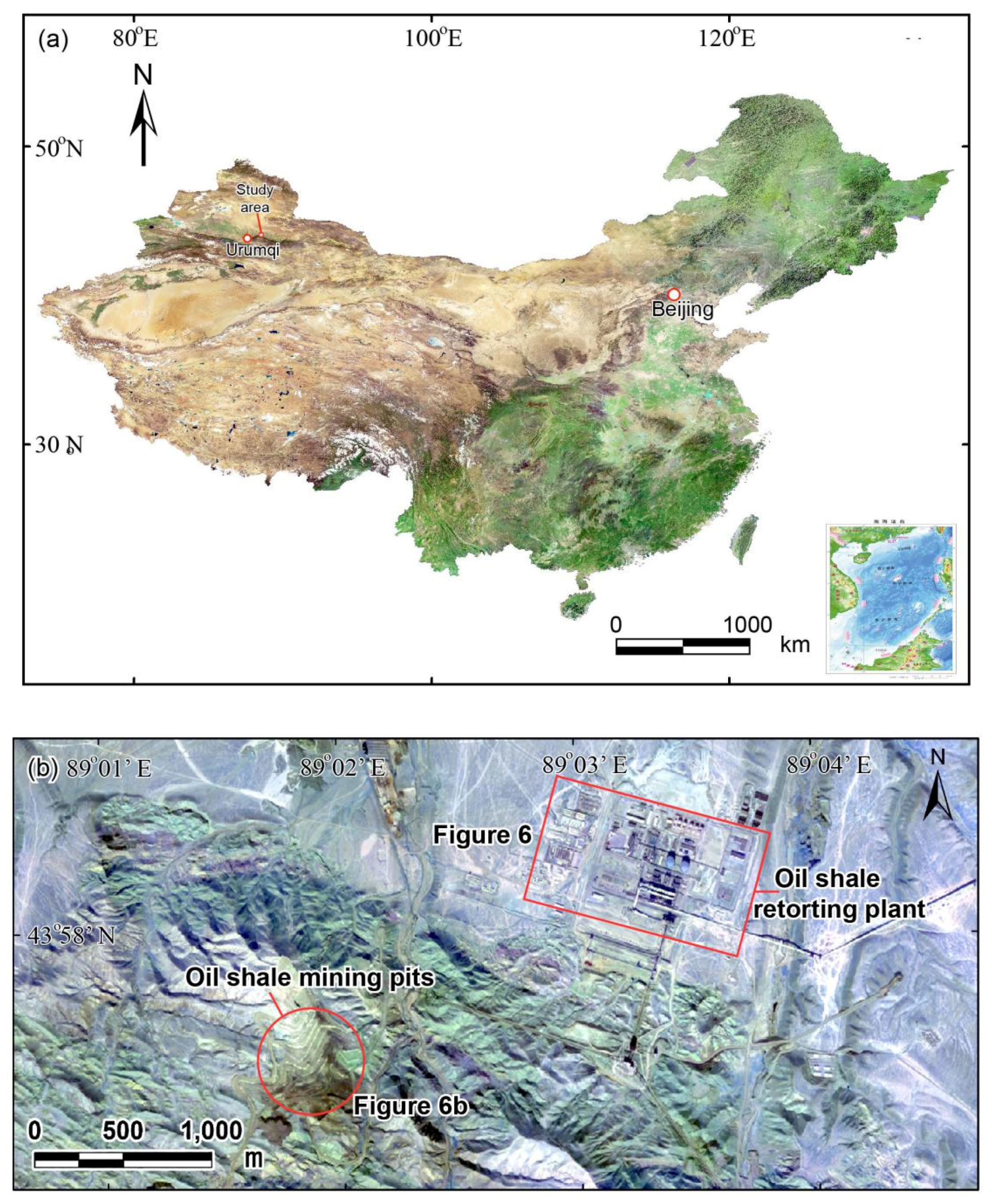
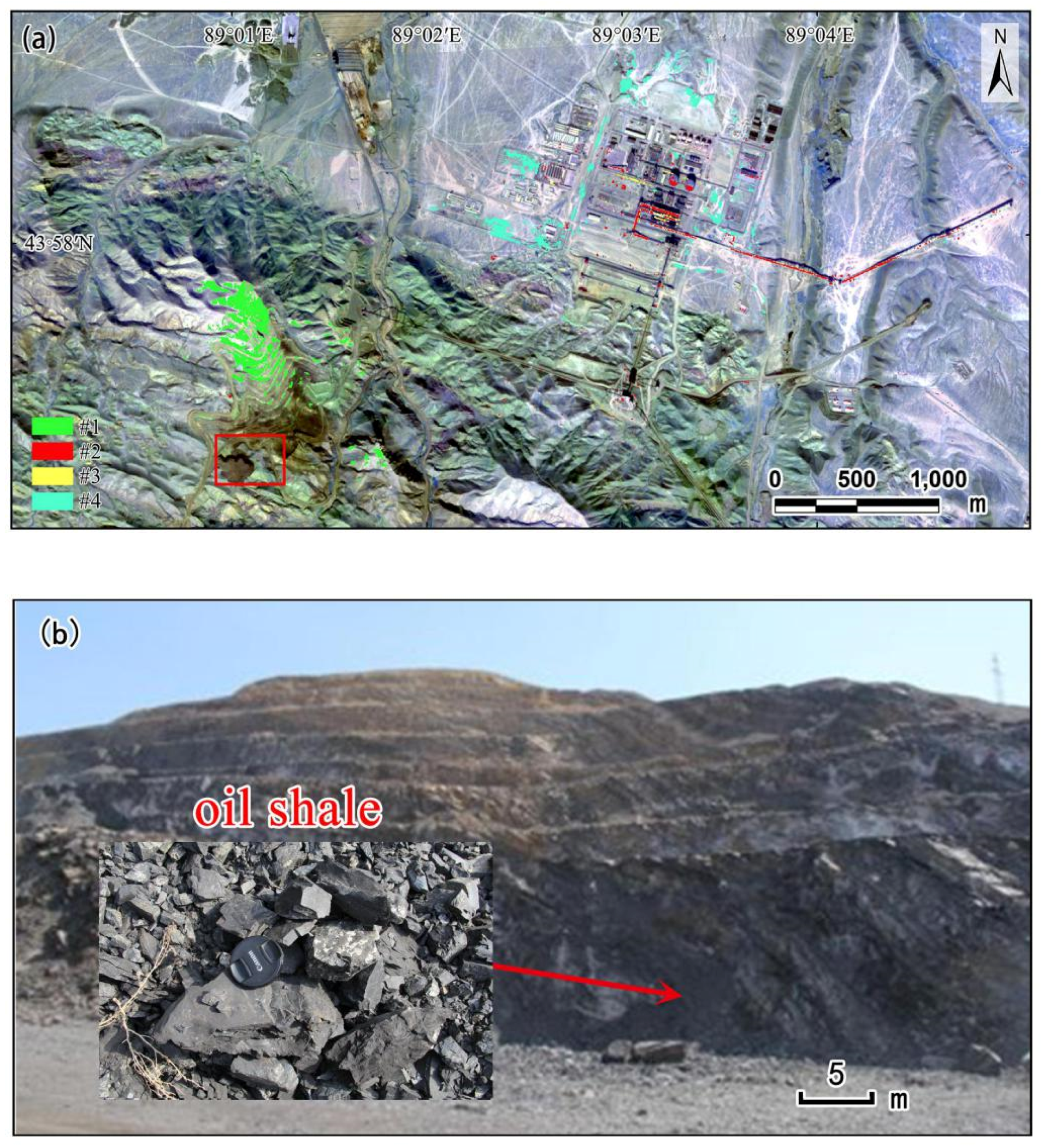
2.1. Study Area

The oil shale mining and retorting area (Figure 1) which are in the southeastern Junggar basin, have been selected as the experimental area. The mine is an open-pit oil shale mine with an annual output of 11 million tons of raw ore, its oil content ranges from 3.71%–9.87%, and the oil shale distillation plant has an annual output of 478,000 tons of shale oil. The test site is located in the arid part of northwest China, where is sparsely populated and surface covered by the Gobi and Desert with sparse vegetation coverage. Therefore, the potential CH₄ release sources in such area is relatively simple, and suited to the research for detecting the sources of CH₄ emissions.

There are two potential types of CH₄ emission sources in the study area. (1) First is the oil shale ore body. On one hand, the CH₄ absorbs onto or is free from the silt rock intercalations in the form of free gas; on the other hand, the oil shale pore absorbed CH₄ are mainly in mesopore and macropore stages. Organic pores are not developed, also the main parts of the oil shale pores are formed by large-scale clay mineral pores [21]. Therefore, CH₄ enrichments in oil shale are mainly in a free state. (2) The second potential source is the oil shale retorting plant. This component of CH₄ is released from the breaking of bonds between aryl methyls or aralkyls during the pyrolysis of oil shale [22,23], according to the reaction equation [23] with measurement coefficient based on the pyrolysis mechanism of oil shale, CH₄ emissions from oil shale smelting are about 277.2 tons per year, an aggregate flux of 759 kg/d is also estimated.

2.2. SASI Data and Preprocessing

SASI is an airborne imaging spectrometer that measures the radiance between 950 nm and 2450 nm in 100 contiguous spectral bands with a nominal full-width half-maximum (FWHM) of 15 nm and a spectral sampling interval of 15 nm. The SASI data used in this study were acquired by flying 1.5 km a.g.l, at the average flight speed of 240 km/h, with an instantaneous field of view (IFOV) of 0.07° and an angular swath width of 40°. The spatial resolution of the data is 2 m, and the signal-to-noise ratio is greater than 1100. The data acquisition system was also equipped with GPS (Global Positioning System)/INS (Inertial Navigation System) sensors to obtain position and attitude data. The airborne data was acquired from 12:07 to 12:26 p.m. (Local time) on 30 September 2013. It was a sunny day in 22 °C, average wind speed was 4 km/h, with a direction of 9° when reached maximum wind speed.

SASI data were radiometrically calibrated using the Speccorr software and were georectified using the Geocor software. Radiance data were converted to W·sr⁻¹·µm⁻¹·m⁻², SASI reflectance data were computed using a bilinear regression method, obtained by (1) measuring the digital number (DN) and reflectance data of black and white cloth (as light and shaded objects, on the ground during aero data acquisition) with an ASD FieldSpec spectrometer (Analytical Spectral Devices Inc., Boulder, CO, USA) in field; (2) resampling the DN data and reflectance data for the black and white cloth to SASI spectral intervals; and (3) using linear interpolation (Formula (1)) to calculate the SASI reflectivity data.

$$\begin{array}{l}{\mathrm{Ref}}_{\mathrm{C}}=\mathrm{a}\cdot {\mathrm{DN}}_{\mathrm{C}}+\mathrm{b}\\ \mathrm{a}=\frac{{\mathrm{Ref}}_{\mathrm{A}}-{\mathrm{Ref}}_{\mathrm{B}}}{{\mathrm{DN}}_{\mathrm{A}}-{\mathrm{DN}}_{\mathrm{B}}}\\ {\mathrm{Ref}}_{\mathrm{C}}=\mathrm{a}\cdot {\mathrm{DN}}_{\mathrm{C}}+\mathrm{b}\end{array}$$

(1)

where white/black cloths are objects A/B, and C is any pixel on the SASI image; DN_A and DN_B are the digital number of objects A and B obtained via the ASD measurement, DN_C is the digital number of any pixel in the SASI image; Ref_A and Ref_B are the respective reflectance of objects A and B measured by ASD, and Ref_C is the reflectance of any pixel of the SASI image; and a/b is the inherent gain and bias of the sensor.

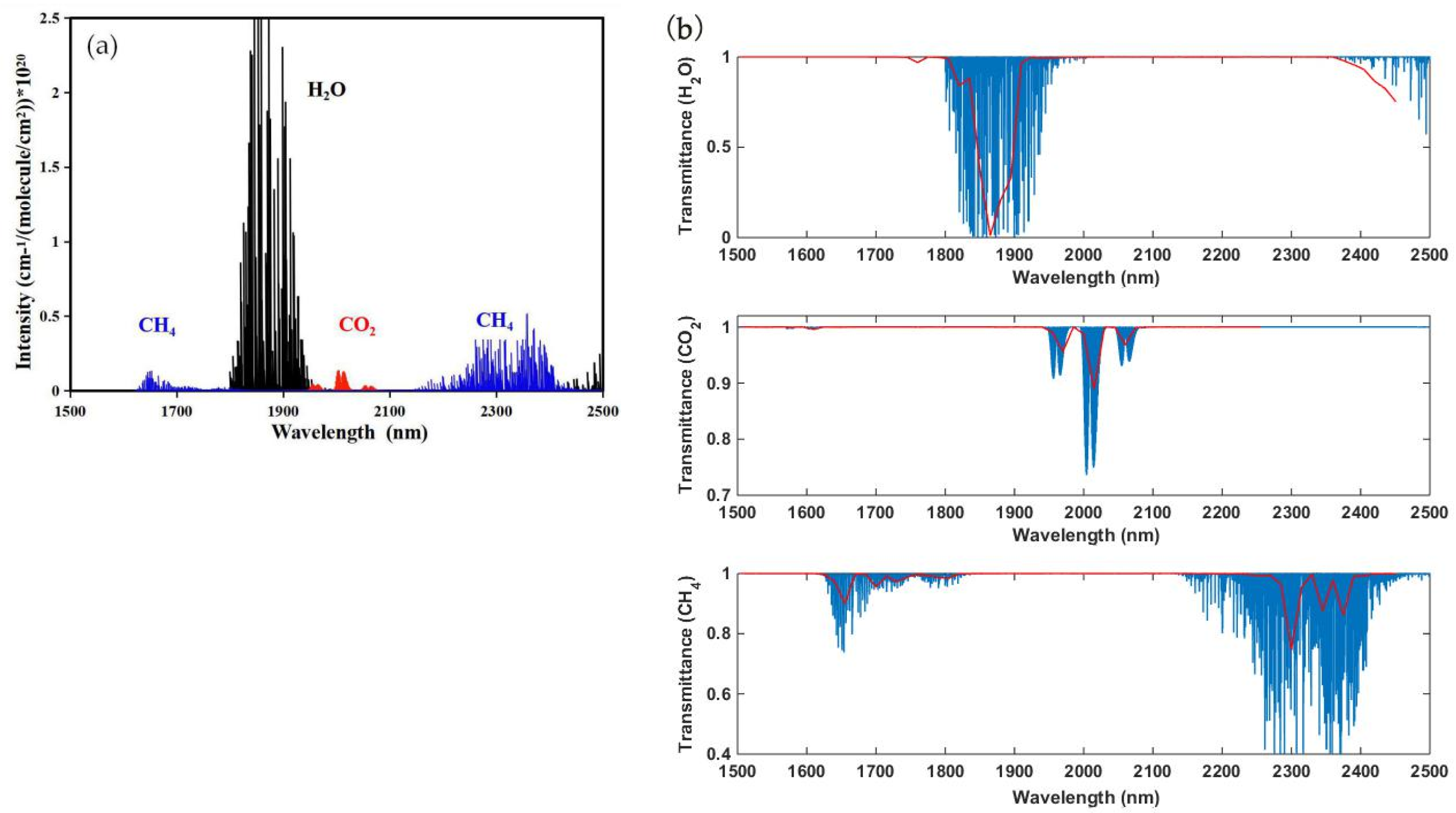
2.3. Band Ratio for CH₄ Emission Detection

Several researchers have successfully used shortwave infrared (SWIR) spectra to detect CH₄ [24,25,26]. The SWIR has a lower amount of saturation over the full atmospheric path, due to the lower SWIR CH₄ absorption coefficients, thereby providing greater sensitivity to CH₄ in the lower atmosphere [24]. CH₄ has fundamental vibrational absorptions in SWIR spectrum, according to the CH₄, CO₂ and H₂O absorption coefficients calculated at a 1-nm spectral interval from spectral lines in the HITRAN database (Figure 2a). CH₄ has strong absorptions between 2200 nm and 2400 nm and a second set of weaker absorptions near 1674 nm. CO₂ also has three significant absorptions in the spectral region at 1970 nm, 2010 nm, 2060 nm, as well as several weaker absorptions centered near 1600 nm. H₂O, the greenhouse gas with the largest radiative forcing [27], have absorptions located in 900 nm, 940 nm, 970 nm, 1130 nm, 1380 nm and 1870 nm. Although SASI are not designed for mapping CH₄ emissions, the sensor’s spectral imaging band covers a range of 950 nm to 2450 nm, which include the absorption features of CH₄ in SWIR (Figure 2b), makes it possible to detect CH₄ emissions.

The aim of this paper is to set up a simple and effective index for detection of anomalous CH₄ emission sources over wide areas that does not rely on the auxiliary ground professional experiments. An alternate remote sensing approach for CH₄ emissions detection is band ratio analysis, such as that used for fire detection [28], which has low computational demands and does not depend on atmospheric and surface parameterizations. Due to the wavelength dependence of atmospheric gas absorption coefficients, negative anomalies in the band ratio images can be indicative of increased gas absorption at the numerator wavelength or decreased gas absorption for the denominator. In this study, the band ratio namely R_CH4, has the form:

R_CH4 = R_absorbing/R_window

(2)

Here, R_absorbing is the radiance data at the CH₄ absorptions band, and R_window is the radiance data at the CH₄ window band.

It is necessary to note that the band ratio method uses the SASI radiance data that include the radiance of ground objects and atmospheric path radiance (Formula (3)) [29]. Radiance data were not processed by atmospheric correction, also reserved the radiation contribution of atmospheric CH₄. The radiance curves show obvious absorption valley characteristics near the absorption bands of CH₄ and H₂O etc., because the scattering effect of atmospheric aerosols and molecules makes the spectrum curve show strong radiation values in the short wavelength.

$$\begin{array}{l}L=\frac{\rho E\tau }{\pi }+L_P\\ L_G=\frac{\rho E}{\pi }\end{array}$$

(3)

where L is total radiance measured by the sensor; L_P is atmospheric path radiance; L_G is radiance of ground object; ρ is reflectance of the ground object; τ is atmospheric transmittance; E is irradiance of ground object.

CH₄ atmospheric window is the spectral bands with transmittance close to 1, such as the transmittance spectra in 2100–2150 nm as shown in Figure 2b. CH₄ atmospheric window band with less absorption influence of CO₂ and H₂O should be selected for band ratio calculation. It is critical to obtain CH₄ absorption band (without interference of other information) from the absorptions window between 2200 nm and 2400 nm, as shown in Figure 2b, using the spectral analysis method. This study determines the absorption characteristic band of CH₄ by the singularity detection processed with a wavelet transform [30,31], which is performed through four steps (Figure 3):

(1)

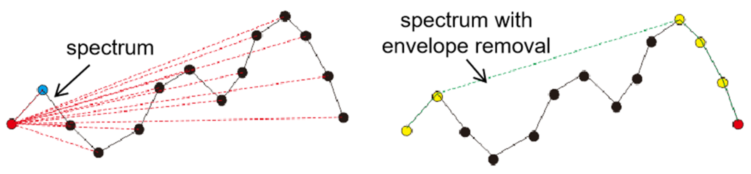
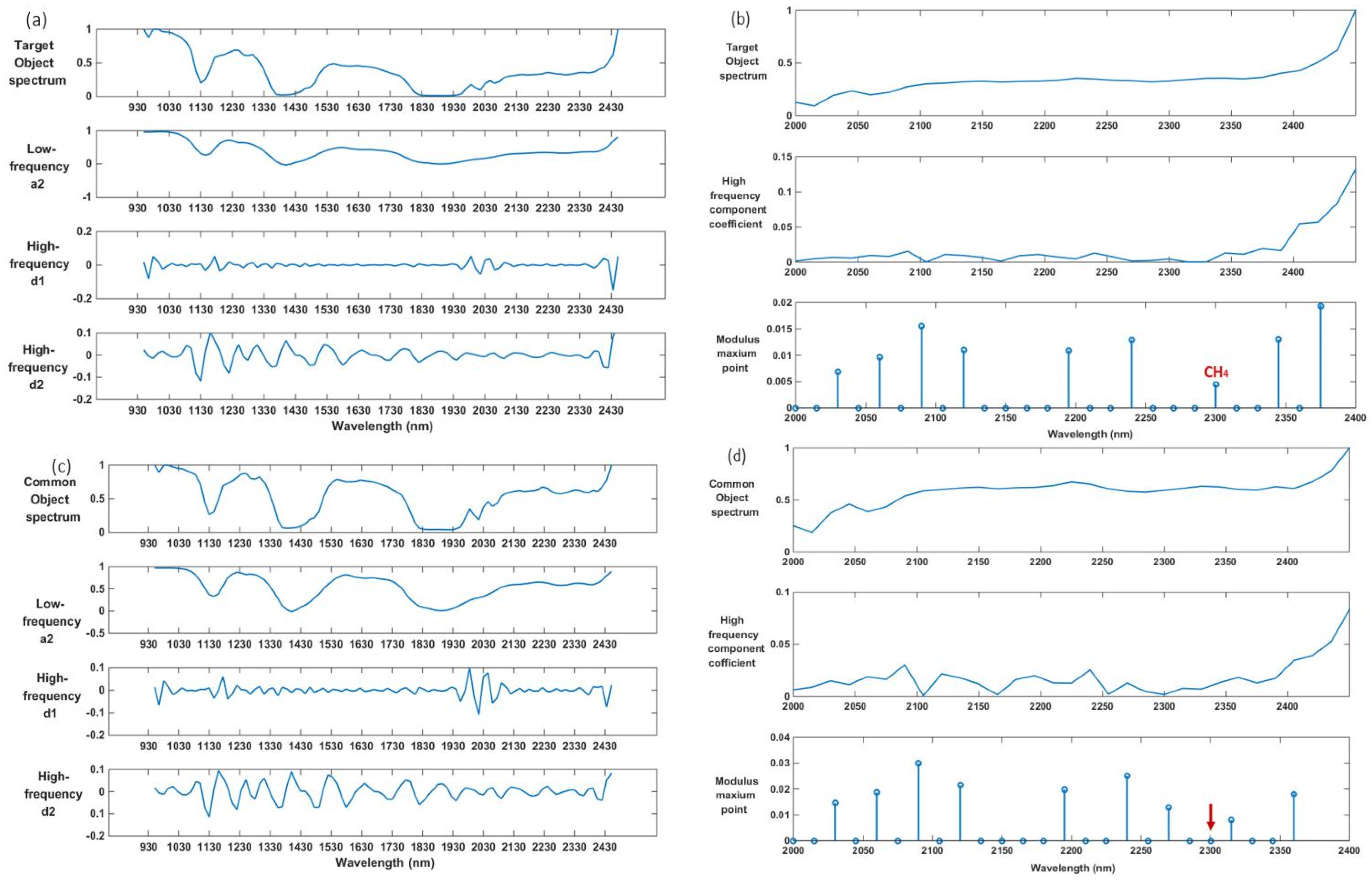
Processing the spectrum with envelope removal can effectively highlight the absorption, reflection and emission characteristics of the spectral curve, and can normalize them to a consistent spectral background, which is conducive to the comparison of characteristic values with other spectral curves [32]. First is the envelope calculation of the spectral curve. Starting from the first point of the spectral curve, this is performed with the various points behind the attachment. The slope is calculated to determine the point of the maximum slope, which is the starting point of the next cycle. This is repeated until the last point of the spectrum curve. All slope maximum points are connected to form the envelope. Then, formula 4 is used to calculate the envelope-removed radiance (Figure 4).

R_ER = R_λ/R_Eλ

(4)

where R_ER is the envelope-removed radiance at the wavelength λ; R_λ is the radiance at the wavelength λ; and R_Eλ is the envelope radiance at the wavelength λ.

(2)

The spectral curve is decomposed using the db5 wavelet [33,34]. Once the wavelet components are computed, the noise is concentrated at the lowest scales while the continuum remains at the highest scales.

(3)

The second layer high-frequency component is obtained after wavelet decomposition, and then the high-frequency component coefficient is calculated. The first layer of the high frequency component coming from the wavelet transform descomposition is the interference information for an extremely strong signal. The absorption features of CH₄ are characterized by weak information. Weak information is easily lost after wavelet decomposition of the third layer. As such, the second layer of the high frequency component from wavelet decomposition will be used to characterize the detailed information of the spectral curve.

(4)

The singularity is detected to obtain the CH₄ absorption bands, by calculating the modulus maximum of the second layer high-frequency component coefficient [30].

2.4. Extraction Method of the CH₄ Release Source

The band ratio method can be used to detect sources of elevated CH₄ release. However, for the extraction of weak information, including free CH₄ release in the oil shale deposit or CH₄ microseepage in the petroliferous basin, it is necessary to analyze the spectral diagnostic features of the surface reflectance to detect the CH₄ source. The method of mineral mapping and classification was adapted for the extraction of surface CH₄ release. The spectral angle mapper (SAM), as a spectral matching method, has been widely used in lithological type identification and mapping using hyperspectral data [35]. However, the conventional mineral mapping uses a mean reflectance spectrum for a specific lithological type [36,37], which does not take into account the spectral variability, is not suitable for multi-objective information extraction. The CH₄ release source as target object of this study, has different types including oil shale, ore beds, the dry distillation plant, etc. Therefore, the method of SAM with a multi-reference spectrum was applied to extract information.

The proposed SAM algorithm can be summarized as follows. Each target spectrum was compared with reference spectra. Their similarities were determined by calculating the angle between the target and the reference spectra. Each pixel was regarded as an n-dimensional vector. Thus, calculating the angle between two spectrums is equivalent to calculate the angle between two vectors (Formula (5)). After all the spectral angles θ between a target spectrum and each reference spectrum were calculated, the minimum angle of all these spectral angles was considered as the definite spectral angle. If the angle between the target pixel and reference spectra was less than the definite spectral angle, the target pixel was identified as belonging to a class. Otherwise, the pixel was identified as not belonging to that class.

$$\theta ={\cos }^{-1}\left\{\frac{{\displaystyle \sum _{i=1}^n{t}_i\cdot r_i}}{{\left[{\displaystyle \sum _{i=1}^n{t}_i^2}\right]}^{1/2}{\left[{\displaystyle \sum _{i=1}^n{r}_i^2}\right]}^{1/2}}\right\} \theta \in \left[0,\frac{\pi }{2}\right],$$

(5)

where it is the target spectrum; r is the reference spectrum; n is the number of wave bands; and θ is the threshold, which is used to determine whether it belongs to the category or component represented by the reference spectrum.

Given that the image spectra are ideal reference spectra in SAM classification [38], image spectra were used in this study. Reference spectra were determined by selecting image spectrum similar to those of ground samples. Spectral reflectance measurements of ground measured spectrum using ASD FieldSpec spectrometer, were carried out in in known gas and oil field of the Junggar basin. Sample spectrum were collected from the spectrum of surface topsoil with CH₄ content higher than 300 uL/Kg.

3. Results

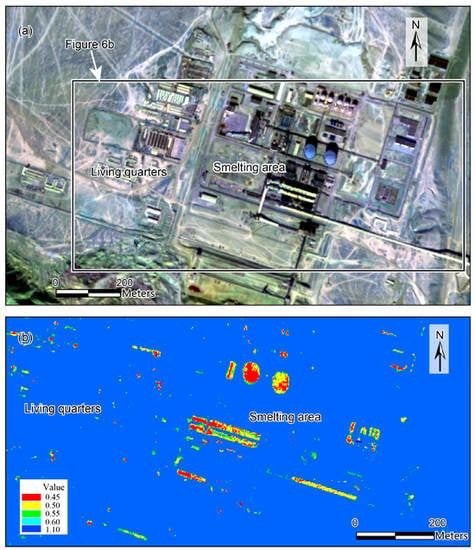
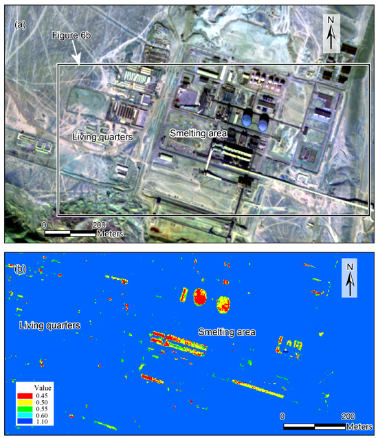
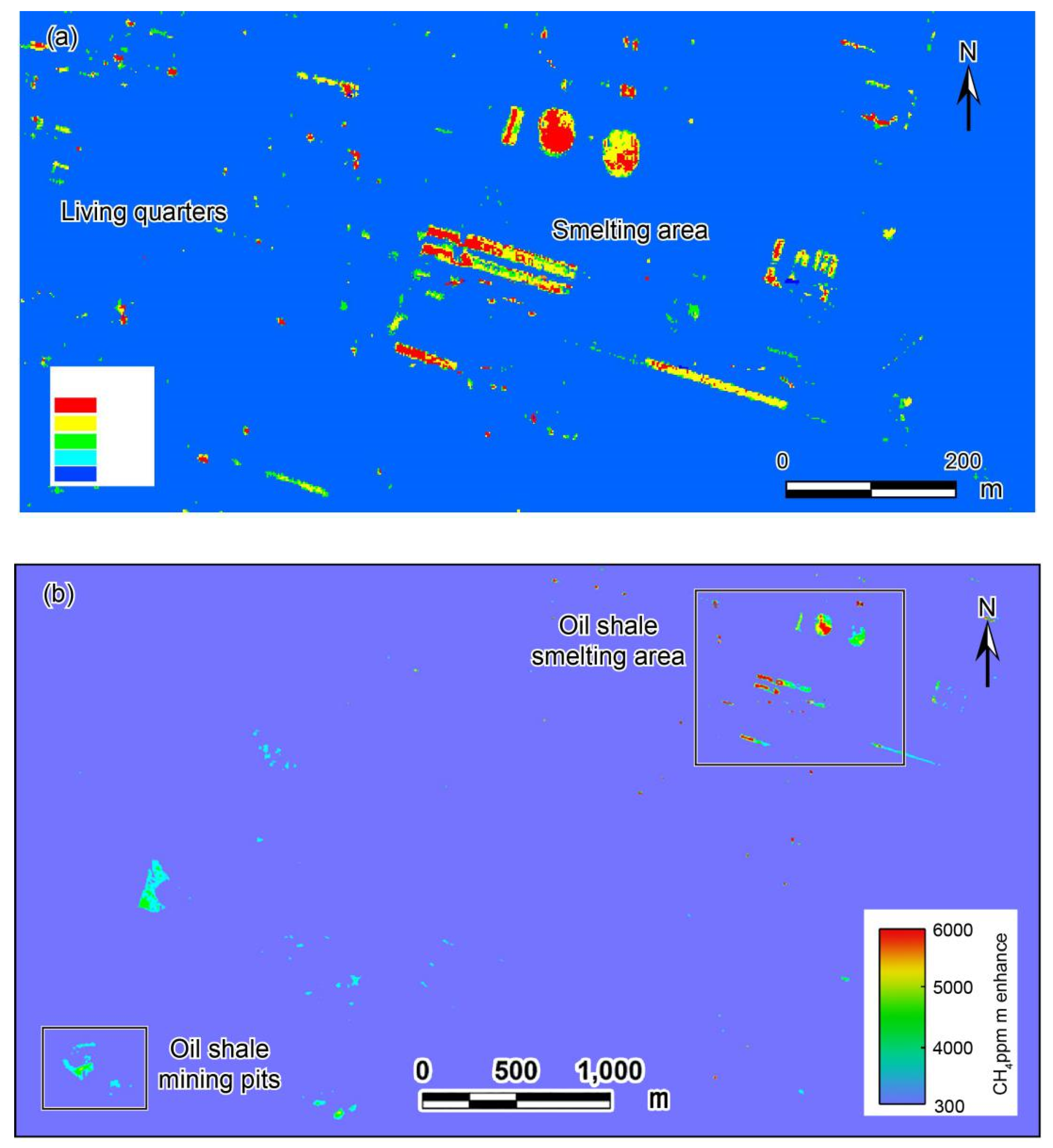
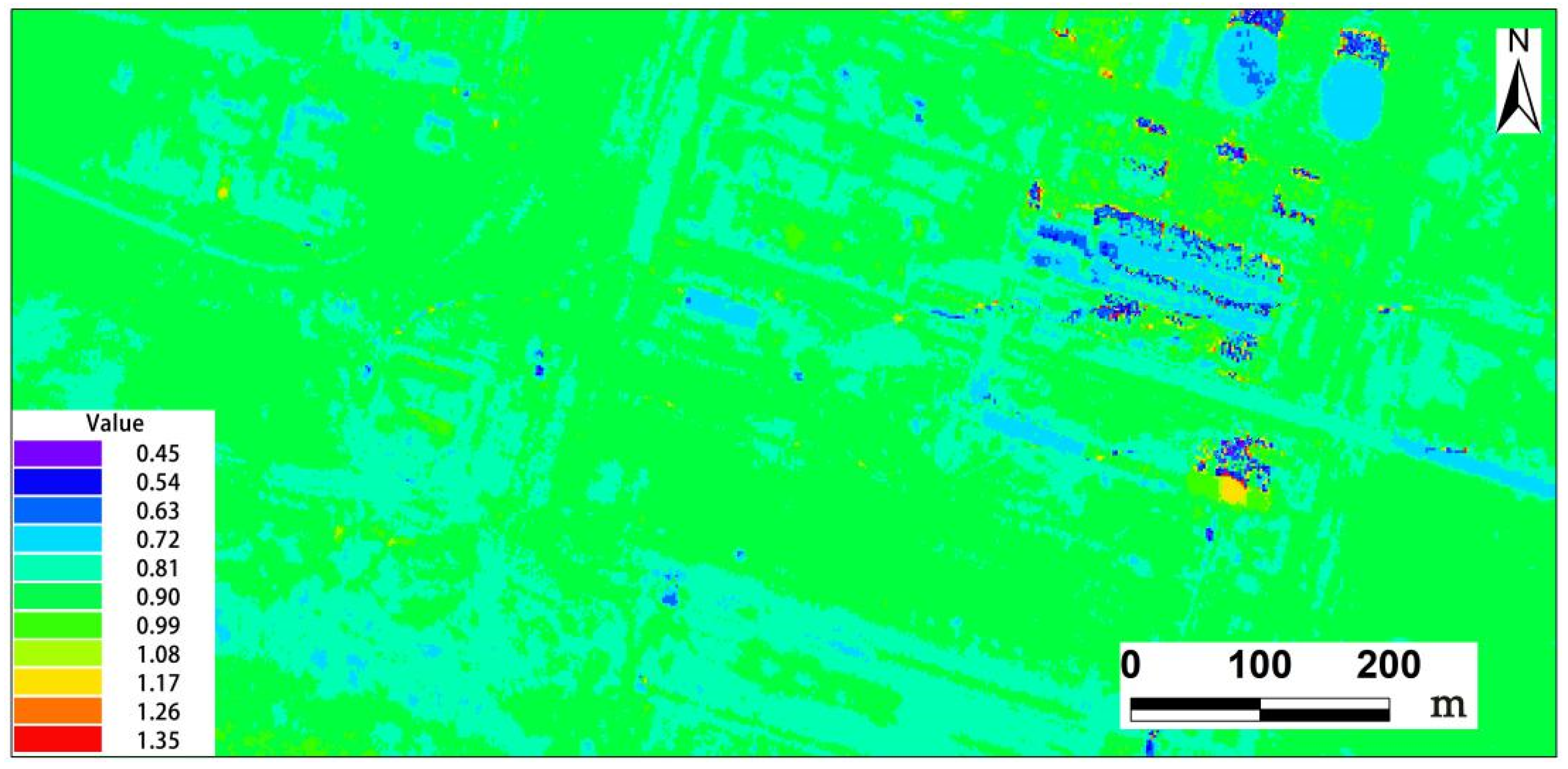
3.1. SASI Radiance Ratio Image for CH₄ Emission Detection

The absorption features of CH₄ near 1700 nm in the short-wave infrared spectrum are weaker than those at 2200–2400 nm, and it is affected by the absorption characteristics of CO₂, as shown in Figure 2. Thus, the bands between 2000 nm and 2400 nm were used to detect the characteristic wavelength of CH₄ absorption. The radiance curve of CH₄ release sources from hydrocarbon storage tanks [13,39] (target objects) and common objects conduct singularity detection processed with wavelet transform at the range between 2000 nm and 2400 nm. The spectral curve of target objects and common objects were decomposed into two layers using the db5 wavelet, from which high-frequency information d1 and d2 were obtained, as shown in Figure 5. The high-frequency information highlights the details of the spectral curve, but the decomposed high frequency component d1 has noise interference, thus, the decomposed high frequency component d2 was used to characterize the detailed information for the spectral curve, and to calculate the high frequency component coefficient cd2. The modulus maximum point calculated by cd2 is shown in Figure 5, namely, the singularity of the spectral curve, is the characteristic absorption band used for ratio calculation.

Three singularities were detected respectively at the wavelengths of 2300 nm, 2345 nm and 2375 nm. The wavelengths of 2345 nm and 2375 nm were not considered, due to H₂O absorption. The band less affected by CO₂ and H₂O absorption at wavelengths of 2105 nm was selected as CH₄ window band. Hence the band ratio was finalized as:

C = R_absorbing/R_window = Band₉₁/Band₇₈ = Radiance_{(2300 nm)}/Radiance_{(2105 nm)}

(6)

According to the results of the band ratio calculation (Figure 6a), the elevated CH₄ locations were mainly distributed in the industrial smelting area. However, no such features were observed in the normal employee living quarters, where building materials are consistent with the distillation zone (Figure 6a). The band ratio created in this study could effectively detect the sources of CH₄ emissions from the oil shale retorting plant. The values (Figure 6b) show local CH₄ enhancement in ppm·m [16], reveals the sources were mainly distributed in areas of oil shale mining and the retorting plant area (as shown in Figure 1b SASI color composite image).

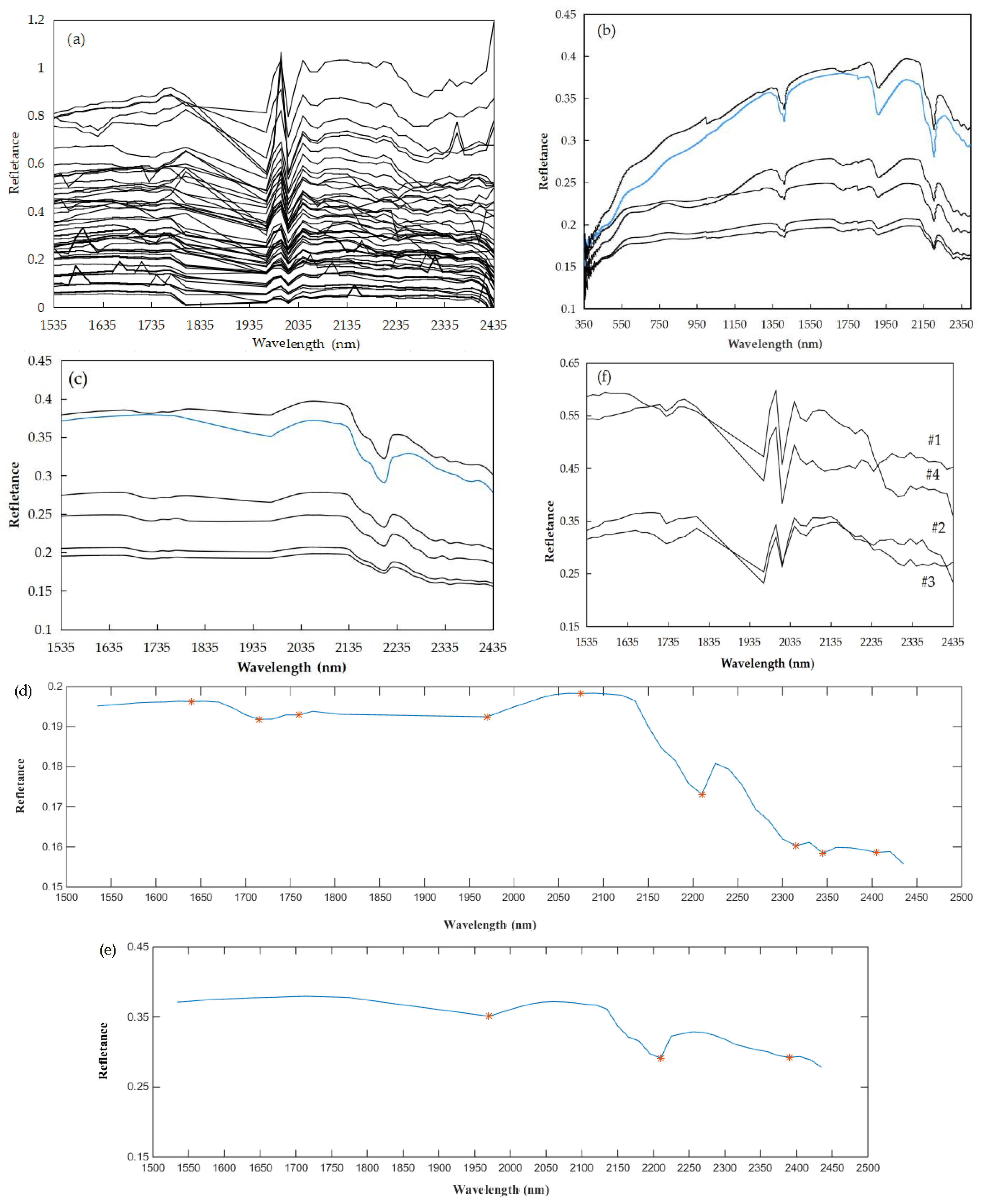
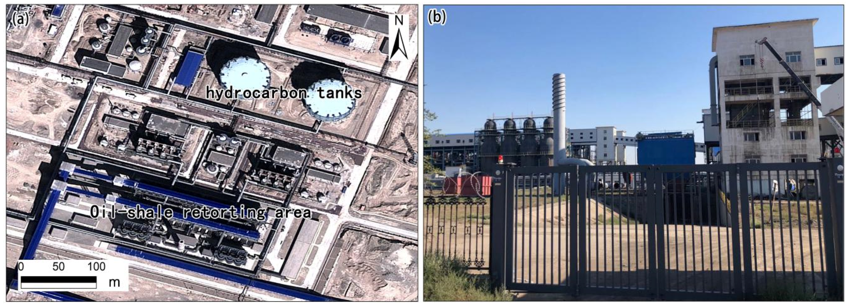
3.2. CH₄ Release Source Extracted from SASI Reflectance Data

For extracting the image spectrum, we used the minimum noise fraction (MNF) algorithm and pixel purity index (PPI) algorithm [40] on SASI reflectance images for the spectral reduction and spatial reduction respectively. In order to realize this method, first, the MNF Rotation tool in Environment for Visualizing Images (ENVI) software were used to reduce the wave band correlation, calculate the data dimension, and obtain the 14 wave bands containing 80% of the information. Then, the pure endmembers were extracted using the Pixel Purity Index (PPI). The 48 endmembers (Figure 7a) extracted with the pixel purity index (PPI) algorithm from the SASI reflectance image.

The process of determining the SAM method’s image reference spectrum as following: First of all, 6 yellow and grey sandy soils spectral curves which measured in the field were selected (Figure 7b). The CH₄ content of soil, which tested by the acid decomposition hydrocarbon analysis, in 5 of them with content of CH₄ higher than 300 uL/kg and the other one is ordinary soil with content of CH₄ 14 uL/kg. Then the spectra minimum of those 6 measured spectra re-sampled to SASI resolution was calculated to determine the position of absorption valley position. By comparing the absorption valleys of the spectral curves of soils with high CH₄ content with those of ordinary soils, the result (Figure 7d,e) shown that there were 3 significant absorptions in the spectral of CH₄-enriched soil region at 1730 nm, 2315 nm and 2345 nm. According to those absorption characteristics, 4 pure endmembers were selected as the reference spectra (Figure 7f) for the SAM classification.

Intra-class spectral angles for four classes are shown in

Table 1. Intra-class spectral angles between samples (all in radian).

Class	Mean Angle	Standard Deviation
1	0.1	0.0082
2	0.1	0.0085
3	0.1	0.0086
4	0.1	0.0173

, and the mapping results are shown in Figure 8a. It can be seen from the mapping results that according to the more typical reference spectra of CH₄ absorption characteristics of 1 and 2, the sources is mainly distributed in the smelting area of the refinery (Figure 8a) and the stepped mining pit (Figure 8b) with oil shale, respectively. It is worth mentioning that in the mapping results, there is no information of CH₄ source in test trenches for exploration oil shale, as seen in the red box area in Figure 8a, because trenches only dug to look for oil shale ore, rather than the distributed oil shale ore, so apparently not CH₄ source, indicating the effectiveness of this classification method.

4. Discussion

The difference with the previous ratio method [19,20] was that the band ratio R_CH4 employed radiance data with envelope removal process. The spectral characteristic curve with envelope removal highlighted the absorption characteristics, the weakened of the influence of environmental factors, and it was more conducive to the analysis of spectral absorption characteristic parameters. Furthermore, wavelet transform singularity detection was adopted to determine the spectral characteristics of the CH₄ absorption band. Base on above mentioned methodology, it was compared with the reflectivity ratio method [20], the radiance ratio R_CH4 reduced the reflection interference of different terrain and surface objects as shown in Figure 9.

The airborne data, which acquired from 12:07 to 12:26 p.m. (Local Time), was used for CH₄ source detection under favorable parameters. The Sun was at its maximum, and so it was the incidence angle and diminishing the scattering of solar radiation. Also, the relative humidity was 31%, the interference of atmospheric components (H₂O) was low, all above which were favorable for CH₄ detection. However, it seems that the low wind speed (4 km/h) was insufficient to disperse the plume at the time of survey. Therefore, the pixels of the plume were concentrated in a few pixels in the image. The Google Earth close-up shown in Figure 10a indicates oil shale smelting area as the likely emission source, which was confirmed by the ground validation by using a thermal imaging camera (FLIR GF320), which is for VOC (volatile organic compounds) detection. The thermal imaging camera (FLIR GF320) is able to detect the CH₄ emissions plume only when the CH₄ concentration is no less than 5000 PPM. Video S1 (see Supplementary Materials) was acquired on 8 August 2019 at around 9:00 a.m. (Local Time) and clearly shown that CH₄ plumes originating at the top of the oil-shale retorting tower (Figure 10a). Therefore, the elevated CH₄ distribution results could be extracted by using the band ratio method are highly consistent with the oil shale smelting area.

Moreover, there were two types of adsorbents CH₄ mapped using SAM classification method with multiple reference spectra, as shown in Figure 8a, the CH₄ emitted by artificial and natural source had certain separating ability. The natural sources of micro-releases mainly include the oil shale deposits and ore beds (Figure 8b), which mainly contained the adsorbed free CH₄. The anthropogenic source was mainly in the dry distillation plant of the oil shale. For example, the CH₄ was in a certain level of emitting from the hydrocarbon floating roof tanks due to various reasons, such as air flows on the tank roof, change of solar radiation and pressure etc. On the other hand, CH₄ was released due to the breaking bonds of either aryl methyls or aralkyls during the pyrolysis of oil shale.

Those results provided the potential mitigations to constrain regional greenhouse gas budgets. Because of a simple band index could identify the target location of unknown CH₄ emitters. Thus, the emission source such as oil-shale retorting tower and hydrocarbon tank can be inspected accurately by using ground thermal infrared detector. Moreover, the categorization of artificial and natural sources could improve partitioning between anthropogenic and natural emission sources to understand the controlling parameters.

5. Conclusions

In this study, a proposed band ratio (namely R_CH4, R_CH4 = Band91_{(2300 nm)}/Band78_{(2105 nm)}) approach using SASI radiance image data which combined with wavelet transform singularity determination, in the image was developed to detect CH₄ emissions sources. The R_CH4 images presented the elevated CH₄ locations, which was consistent with the distribution of the oil shale smelting area, verified by high-resolution Google Earth imagery and thermal imaging camera (FLIR GF320). It is concluded that the R_CH4 proposed by this study could be useful for the detecting ambiguous CH₄ emission sources.

In addition, SASI surface reflectance data and multiple reference spectra in SAM were used to extract the distribution of surface CH₄ release sources. This method accounts for the spectral variability of different sources. Four image reference spectra with absorption characteristics near 1730 nm and 2315 nm were selected to effectively extract four types of ground objects enriched with CH₄ by referring to the spectral diagnostic characteristics of soil enriched with CH₄. The results shown that there were two types of CH₄ release sources in the study area. Natural release sources include oil shale ore body, which was enriched with CH₄ in a free state. There are also anthropogenic CH₄ sources that include the oil shale retorting plant, where CH₄ was released due to the breaking of bonds between aryl methyls or aralkyls during the pyrolysis of oil shale. They could be spectrally differentiated, for which imaging spectrometer data can provide a unique spatial characterization of concentrated CH₄ emissions. Hence, the CH₄ emission sources from natural or artificial sources could be identified in a local-scale.

As an important greenhouse gas, CH₄ does not persist in the atmosphere as long as CO₂ does, but its warming effect is much stronger. Therefore, the sources of CH₄ release must be documented in detail to take control measures for reducing CH₄ emissions. SASI has the high spatial resolution to resolve small-scale emissions and could map the large region quickly, permitting unambiguous identification of individual emission source locations, and verification of a number of emission sources such as oil shale retort presented using a thermal camera. This study demonstrated that the utility of SASI system, can indeed provide an effective local-scale approach for detecting the CH₄ emission sources related to hydrocarbon development.

References

1. IPCC. Climate Change 2013: The Physical Science Basis. In Contribution of Working Group I to the Fifth Assessment Report of the Intergovernmental Panel on Climate Change; Stocker, T.F., Qin, D., Plattner, G.K., Tignor, M., Allen, S.K., Boschung, J., Nauels, A., Xia, Y., Bex, V., Midgley, P.M., Eds.; Cambridge University Press: Cambridge, UK; New York, NY, USA, 2013; p. 1535. [Google Scholar]
2. Saunois, M.; Jackson, R.B.; Bousquet, P.; Poulter, B.; Canadell, J.G. The growing role of methane in anthropogenic climate change. Environ. Res. Lett. 2016, 11, 120207. [Google Scholar] [CrossRef] [Green Version]
3. Nisbet, E.G.; Dlugokencky, E.J.; Bousquet, P. Methane on the rise—Again. Science 2014, 343, 493–495. [Google Scholar] [CrossRef] [PubMed] [Green Version]
4. Anenberg, S.C.; Schwartz, J.; Shindell, D.; Amann, M.; Faluvegi, G.; Klimont, Z.; Janssens-Maenhout, G.; Pozzoli, L.; Van Dingenen, R.; Vignati, E.; et al. Global air quality and health co-benefits of mitigating near-term climate change through methane and black carbon emission controls. Environ. Health Perspect. 2012, 120, 831–839. [Google Scholar] [CrossRef] [PubMed] [Green Version]
5. Lelieveld, J.O.S.; Crutzen, P.J.; Dentener, F.J. Changing concentration, lifetime and climate forcing of atmospheric methane. Tellus B 1998, 50, 128–150. [Google Scholar] [CrossRef]
6. Hausmann, P.; Sussmann, R.; Smale, D. Contribution of oil and natural gas production to renewed increase of atmospheric methane (2007–2014): Top-down estimate from ethane and methane column observations. Atmos. Chem. Phys. 2016, 15, 35991–36028. [Google Scholar] [CrossRef] [Green Version]
7. Hansen, J.; Sato, M.; Ruedy, R.; Lacis, A.; Oinas, V. Global warming in the twenty-first century: An alternative scenario. Proc. Acad. Natl. Sci. USA 2000, 18, 9875–9880. [Google Scholar] [CrossRef] [Green Version]
8. Frankenberg, C.; Meirink, J.F.; van Weele, M.; Platt, U.; Wagner, T. Assessing methane emissions from global space-borne observations. Science 2005, 308, 1010–1014. [Google Scholar] [CrossRef] [Green Version]
9. Roberts, D.A.; Bradley, E.S.; Cheung, R.; Leifer, I.; Dennison, P.E.; Margolis, J.S. Mapping methane emissions from a marine geological seep source using imaging spectrometry. Remote Sens. Environ. 2010, 114, 592–606. [Google Scholar] [CrossRef]
10. Schneising, O.; Buchwitz, M.; Reuter, M.; Heymann, J.; Bovensmann, H.; Burrows, J.P. Long-term analysis of carbon dioxide and methane column-averaged mole fractions retrieved from SCIAMACH. Atmos. Chem. Phys. 2011, 11, 2863–2880. [Google Scholar] [CrossRef] [Green Version]
11. Gerilowski, K.; Tretner, A.; Krings, T.; Buchwitz, M.; Bertagnolio, P.P.; Belemezov, F.; Erzinger, J.; Burrows, J.P.; Bovensmann, H. MAMAP—A new spectrometer system for column-averaged methane and carbon dioxide observations from aircraft: Instrument description and performance analysis. Atmos. Meas. Tech. 2011, 4, 215–243. [Google Scholar] [CrossRef] [Green Version]
12. Krings, T.; Gerilowski, K.; Buchwitz, M.; Hartmann, J.; Sachs, T.; Erzinger, J.; Burrows, J.P.; Bovensmann, H. Quantification of methane emission rates from coal mine ventilation shafts using airborne remote sensing data. Atmos. Meas. Tech. 2013, 6, 151–166. [Google Scholar] [CrossRef] [Green Version]
13. Thorpe, A.K.; Frankenberg, C.; Thompson, D.R.; Duren, R.M.; Aubrey, A.D.; Bue, B.D.; Green, R.O.; Gerilowski, K.; Krings, T.; Borchardt, J.; et al. Airborne DOAS retrievals of methane, carbon dioxide, and water vapor concentrations at high spatial resolution: Application to AVIRIS-NG. Atmos. Meas. Tech. 2017, 10, 3833–3850. [Google Scholar] [CrossRef] [Green Version]
14. Scafutto, R.D.P.M.; De Souza Filho, C.R. Detection of Methane Plumes Using Airborne Midwave Infrared (3–5 µm) Hyperspectral Data. Remote Sens. 2018, 10, 1237. [Google Scholar] [CrossRef] [Green Version]
15. Buchwitz, M.; Rozanov, V.V.; Burrows, J.P. A near-infrared optimized doas method for the fast global retrieval of atmospheric CH4, CO, CO2, H2O, and N2O total column amounts from sciamachy envisat-1 nadir radiances. J. Geophys. Res. Atmos. 2000, 105, 15231–15245. [Google Scholar] [CrossRef]
16. Thompson, D.R.; Leifer, I.; Bovensmann, H.; Eastwood, M.; Fladeland, M.; Frankenberg, C. Real-time remote detection and measurement for airborne imaging spectroscopy: A case study with methane. Atmos. Meas. Tech. 2015, 8, 4383–4397. [Google Scholar] [CrossRef] [Green Version]
17. Thorpe, A.K.; Roberts, D.A.; Bradley, E.S.; Funk, C.C.; Dennison, P.E.; Leifer, I. High resolution mapping of methane emissions from marine and terrestrial sources using a Cluster-Tuned Matched Filter technique and imaging spectrometry. Remote Sens. Environ. 2013, 134, 305–318. [Google Scholar] [CrossRef]
18. Larsen, N.F.; Stamnes, K. Methane detection from space: Use of sunglint. Opt. Eng. 2006, 45, 016202. [Google Scholar] [CrossRef]
19. Bradley, E.S.; Leifer, I.; Roberts, D.A.; Dennison, P.E.; Washburn, L. Detection of marine methane emissions with AVIRIS band ratios. Geophys. Res. Lett. 2011, 10, 415–421. [Google Scholar] [CrossRef]
20. Zhang, M.W.; Leifer, I.; Hu, C. Challenges in Methane Column Retrievals from AVIRIS-NG Imagery over Spectrally Cluttered Surfaces: A Sensitivity Analysis. Remote Sens. 2017, 9, 835. [Google Scholar] [CrossRef] [Green Version]
21. Cao, T.T.; Song, Z.G.; Luo, H.Y.; Liu, G.X. The difference of microscopic pore structure characteristics of coal, oil shale and shale and their storage mechanisms. Nat. Gas Geosic. 2015, 26, 2208–2218. [Google Scholar]
22. Fuke, D.; Dong, Y.; Zijun, F. Permeability evolution of Jimsar oil shale under high temperature and triaxial stresses. Coal Technol. 2017, 36, 165–166. [Google Scholar]
23. Campbell, J.H.; Gallegos, G.; Gregg, M. Gas evolution during oil shale pyrolysis. 2. Kinetic and stoichiometric analysis. Fuel 1980, 5910, 727–732. [Google Scholar] [CrossRef]
24. Frankenberg, C.; Meirink, J.F.; Bergamaschi, P.; Goede, A.P.H.; Heimann, M.; Körner, S.; Platt, U.; Weele, M.V.; Wagner, T. Satellite cartography of atmospheric methane from SCIAMACHY on board ENVISAT: Analysis of the years 2003 and 2004. J. Geophys. Res. Atmos. 2006, 111, 7. [Google Scholar] [CrossRef]
25. Straume, A.G.; Schrijver, H.; Gloudemans, A.M.S.; Houweling, S.; Aben, I.; Maurellis, A.N.; Laat, A.T.J.D.; Kleipool, Q.; Lichtenberg, G.; Hees, R.V. The global variation of CH4 and CO as seen by SCIAMACHY. Adv. Space Res. 2005, 36, 821–827. [Google Scholar] [CrossRef]
26. Schepers, D.; Guerlet, S.; Butz, A.; Landgraf, J.; Frankenberg, C.; Hasekamp, O.; Blavier, J.F.; Deutscher, N.M.; Griffith, D.W.T.; Hase, F. Methane retrievals from Greenhouse Gases Observing Satellite (GOSAT) shortwave infrared measurements: Performance comparison of proxy and physics retrieval algorithms. J. Geophys. Res. Atmos. 2012, 117, 63–74. [Google Scholar] [CrossRef] [Green Version]
27. Kiehl, J.T.; Trenberth, K.E. Earth’s annual global mean energy budget. Bull. Am. Meteorol. Soc. 1997, 78, 197–208. [Google Scholar] [CrossRef] [Green Version]
28. Dennison, P.E.; Roberts, D.A. Daytime fire detection using airborne hyperspectral data. Remote Sens. Environ. 2009, 113, 1646–1657. [Google Scholar] [CrossRef]
29. Lillesand, T.M.; Kiefer, R.W. Remote Sensing and Image Interpretation, 3rd ed.; John Wiley & Sons: New York, NY, USA, 1994; pp. 7–8. ISBN 0471305758. [Google Scholar]
30. Stephane, M.; Wen, L.H. Singularity detection and processing with wavelets. IEEE Trans. Inf. Theory 1992, 38, 617–634. [Google Scholar]
31. Liu, Y.; Qin, F.; Liu, Y.; Cen, Z. The 2D large deformation analysis using Daubechies wavelet. Comput. Mech. 2010, 45, 179–187. [Google Scholar] [CrossRef]
32. Huang, Z.; Turner, B.J.; Dury, S.J.; Wallis, I.R.; Foley, W.J. Estimating foliage nitrogen concentration from hymap data using continuum removal analysis. Remote Sens. Environ. 2004, 93, 18–29. [Google Scholar] [CrossRef]
33. Xu, Y.; Weaver, J.B.; Healy, D.M.; Lu, J. Wavelet transform domain filters: A spatially selective noise filtration technique. IEEE Trans. Image Process. 1994, 3, 747–758. [Google Scholar] [PubMed] [Green Version]
34. Zhang, X.D.; Younan, N.H.; O’Hara, C.G. Wavelet domain statistical hyperspectral soil texture classification. IEEE Trans. Geosci. Remote Sens. 2005, 43, 615–618. [Google Scholar] [CrossRef]
35. Cho, M.A.; Debba, P.; Mathieu, R.; Naidoo, L.; van Aardt, J.; Asner, G.P. Improving discrimination of savanna tree species through a multiple-endmember spectral angle mapper approach: Canopy-level analysis. IEEE Trans. Geosci. Remote Sens. 2010, 48, 4133–4142. [Google Scholar] [CrossRef]
36. Murphy, R.J.; Monteiro, S.T.; Schneider, S. Evaluating classification techniques for mapping vertical geology using field-based hyperspectral sensors. IEEE Trans. Geosci. Remote Sens. 2012, 50, 3066–3080. [Google Scholar] [CrossRef]
37. Kruse, F.A.; Boardman, J.W.; Huntington, J.F. Comparison of Airborne Hyperspectral Data and EO-1 Hyperion for Mineral Mapping. IEEE Trans. Geosci. Remote Sens. 2003, 41, 1388–1400. [Google Scholar] [CrossRef] [Green Version]
38. Hecker, C.; Vander Meijde, M.; Vander Werff, H.; Vander Meer, F.D. Assessing the influence of reference spectra on synthetic SAM classification results. IEEE Trans. Geosci. Remote Sens. 2008, 46, 4162–4172. [Google Scholar] [CrossRef]
39. Thorpe, A.K.; Frankenberg, C.; Roberts, D.A. Retrieval techniques for airborne imaging of methane concentrations using high spatial and moderate spectral resolution: Application to AVIRIS. Atmos. Meas. Tech. 2014, 7, 491–506. [Google Scholar] [CrossRef] [Green Version]
40. Kruse, F.A.; Boardman, J.W.; Huntington, J.F. Comparison of airborne and satellite hyperspectral data for geologic mapping. Proc. SPIE Int. Soc. Opt. Eng. 2002, 4725, 128–139. [Google Scholar]
Figure 1. (a) Location map of study area; (b) Shortwave Airborne Spectrographic Imager (SASI) color composite image (R: 2420 nm, G: 1730 nm, B: 950 nm) of the study area.
Remotesensing 12 00537 g001
Figure 2. (a) Methane (CH4, blue), carbon dioxide (CO2, red), and water vapor (H2O, black) spectral intensity in the shortwave infrared (SWIR) Spectral Intensity (cm−1/(molecule/cm2)) were derived from HITRAN at a 1-nm spectral interval at 296 K, consistent with ambient temperature of obtaining aviation data; (b) CH4, CO2, and H2O transmittance spectra convolved to SASI (15 nm) spectral resolution. SASI absorptions windows are indicated by the black outlines.
Remotesensing 12 00537 g002
Figure 3. Flow for extracting the absorption bands of CH4 via wavelet transform singularity detection.
Remotesensing 12 00537 g003
Figure 4. Radiance spectrum and radiance spectrum with envelope removal.
Remotesensing 12 00537 g004
Figure 5. The result of wavelet transform singularity detection. (a) The db5 wavelet two-layer decomposition result of a target object spectral curve; (b) The singularity of a target object spectral curve (2000–2400 nm); (c) The db5 wavelet two-layer decomposition result of a common object spectral curve; (d) The singularity of a common object spectral curve (2000–2400 nm).
Remotesensing 12 00537 g005
Figure 6. (a) The band ratio image of the industrial smelting area; (b) The elevated CH4 locations are clearly visible with local CH4 enhancement in ppm·m.
Remotesensing 12 00537 g006
Figure 7. (a) The 48 endmembers extracted with PPI from the SASI reflectance image; (b) The 6 yellow and grey sandy soils spectral curves measured in the field by Analytical Spectral Devices Inc., Boulder, CO, USA (ASD); (c) The 6 yellow and grey sandy soils spectra re-sampled to SASI resolution; (d) The spectra minimum of soils containing CH4 (the content of CH4 was higher than 300 uL/kg); (e) The spectra minimum of soils with the content of CH4 was 14 uL/kg); (f) The reference spectra used for SAM classification.
Remotesensing 12 00537 g007
Figure 8. (a) CH4 release sources mapped from SASI reflectance data; (b) Field photograph showing the oil shale mining pit.
Remotesensing 12 00537 g008
Figure 9. Band ratio (ζ) image of reflectance for the 2300 nm and 2060 nm bands.
Remotesensing 12 00537 g009
Figure 10. (a) Higher-resolution Google Earth imagery (30 September 2013) of the oil-shale retorting plant, showing that the source of elevated CH4 is from oil-shale retorting tower, hydrocarbon tank etc.; (b) Field photograph showing the oil-shale retorting plant.
Remotesensing 12 00537 g010