High Accuracy Geochemical Map Generation Method by a Spatial Autocorrelation-Based Mixture Interpolation Using Remote Sensing Data

Abstract

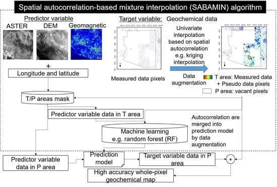
Generating a high-resolution whole-pixel geochemical contents map from a map with sparse distribution is a regression problem. Currently, multivariate prediction models like machine learning (ML) are constructed to raise the geoscience mapping resolution. Methods coupling the spatial autocorrelation into the ML model have been proposed for raising ML prediction accuracy. Previously proposed methods are needed for complicated modification in ML models. In this research, we propose a new algorithm called spatial autocorrelation-based mixture interpolation (SABAMIN), with which it is easier to merge spatial autocorrelation into a ML model only using a data augmentation strategy. To test the feasibility of this concept, remote sensing data including those from the advanced spaceborne thermal emission and reflection radiometer (ASTER), digital elevation model (DEM), and geophysics (geomagnetic) data were used for the feasibility study, along with copper geochemical and copper mine data from Arizona, USA. We explained why spatial information can be coupled into an ML model only by data augmentation, and introduced how to operate data augmentation in our case. Four tests—(i) cross-validation of measured data, (ii) the blind test, (iii) the temporal stability test, and (iv) the predictor importance test—were conducted to evaluate the model. As the results, the model’s accuracy was improved compared with a traditional ML model, and the reliability of the algorithm was confirmed. In summary, combining the univariate interpolation method with multivariate prediction with data augmentation proved effective for geological studies.

1. Introduction

1.1. Background

Geoscience data, which are dependent on the fieldwork of geologists, for example, lithological data, geochemical data, etc., are always sparse on distribution maps. In recent studies, besides conventional univariate geospatial interpolation methods, multivariate prediction models have been constructed to raise the geoscience mapping resolution by using various geoscience data, especially remote sensing data, as predictors. Pal et al. [1] have used fused multi-classifiers, which include multi-spectral data, to achieve high-resolution lithological classification. Kirkwood et al. [2] have applied random forests (RFs) machine learning (ML) methods to generate whole-pixel geochemical contents maps. The data in unknown locations are predicted by the geographical referenced input data containing co-located pixels specified by coordinates linked to a spatial reference frame, which is equivalent to processing the predictions in a geographic space where samples are only compared numerically [3].

Unlike lithological mapping, which is a classification work, a geochemical contents map is like an image with analogue values, thus generating a high-resolution whole-pixel geochemical contents map is a regression problem. It is suggested that considering the geological spatial dependencies, spatial location, and spatial autocorrelation due to geological continuity, it cannot be ignored [4]. Cracknell et al. [5] demonstrated the prediction accuracy raised by treating spatial coordinates as predictors to couple the spatial autocorrelation into the ML model. Sergeev et al. [6] proposed a method to include spatial autocorrelation into an artificial neural network (ANN) by applying a kriging model. However, in their models, ML models are needed for complicated modification.

Therefore, we propose a new algorithm called SABAMIN (spatial autocorrelation-based mixture interpolation) that can merge both spatial location and autocorrelation, which are generated from the univariate geospatial interpolation model into an ML model using a data augmentation strategy [7] to provide a high accuracy model that can generate a high-resolution geochemical map. The data augmentation strategy is currently used for solving small data machine learning, and has proved effective in raising the accuracy of the machine learning model [8,9]. It is only needed to contain pseudo training data generated from a reliable expert model into training datasets, which is an easy task. It has to be noted that the accuracy and reliability of the ML model is determined by the accuracy and reliability of the model for generating the pseudo training data.

In this research, to prove the effectiveness of this concept in geological study, we combine kriging interpolation [10] and RFs to construct our new algorithm as an example. Because kriging interpolation is a well-known method based on the spatial autocorrelation of data in Euclidian space, and RF is an interpretable ML method [11] that has the merit to determine which predictor is important in the model, here, we use kriging interpolation to create pseudo training datasets and RF to construct a prediction model. We explain why both spatial location and autocorrelation can be coupled into an ML model only by data augmentation, as well as how to create reliable pseudo training data in the case of using kriging interpolation. Moreover, we demonstrate the reliability of the algorithm using the example of generating a whole-pixel copper contents distribution map.

A portion of the findings in this report is based on the work [12] presented at the SPIE Remote Sensing 2019 conference. All the data used in this research are open data obtained from the United States Geological Survey (https://lpdaac.usgs.gov).

1.2. Why Spatial Information Can be Coupled into an Ml Model Only by Data Augmentation

In this section, we will explain why both spatial location and autocorrelation can be coupled into an ML model only by data augmentation.

1.2.1. Spatial Information Calculated from Kriging Interpolation

The sampled target variable data points are defined as S_i(x_si,y_si), si = 1, …, N, and vacant points are defined as A_j(x_aj,y_aj), aj = 1, …, M. Here, N and M are the number of total sampled target variable points and vacant pixels, respectively.

In kriging interpolation, two steps are executed in the following order: (i) Construct a spatial distribution model of sampled points using variography; (ii) interpolate the vacant points. In the basic kriging model, the system of equations is shown in Equation (1):

$$\underset{\Lambda }{\min }E={\Lambda }^T·V·\Lambda -C^T·\Lambda -{\Lambda }^T·C+V subject to {\mathbf{1}}^T·\Lambda =1$$

(1)

where E is the variance of prediction errors at vacant points, Λ is the size of an (M × N) matrix whose elements λ_j,i are the weights to the measured value of S_i for interpolating A_j, V is the size of an (N × N) matrix whose elements v_a,b is the variance (here, semivariance is used) within pairs of sampled points S_a and S_b, and C is the size of an (N × M) matrix whose elements c_a,b are the covariance within pairs of sampled points S_a and vacant pixel A_b. To ensure that the model is unbiased, the weights must be summed to one. To obtain the best prediction precision, E should be minimized, which is equivalent to optimization problem results in a kriging system. By using Lagrange multipliers, Λ can be solved by Equations (2) and (3):

$$\left[\begin{array}{c}\Lambda \\ \mu \end{array}\right]={\left[\begin{array}{cc}V& 1\\ {\mathbf{1}}^T& 0\end{array}\right]}^{-1}·\left[\begin{array}{c}C\\ 1\end{array}\right]$$

(2)

$$\Lambda =V^{-1}·C+V^{-1}·{\left(-{\mathbf{1}}^T·V^{-1}\right)}^{-1}·{\mathbf{1}}^T·V^{-1}·C-V^{-1}·{\left(-{\mathbf{1}}^T·V^{-1}\right)}^{-1}$$

(3)

where μ is a Lagrange multiplier used in the minimization of the kriging error to honor the unbiasedness condition. Equation (3) is based on the analytic inversion formula for block-matrix inversion, and when the block matrix is not square, pseudo inversion is used. Then, the vacant pixels are interpolated through Equation (4), which is analogous to inverse distance weighting (IDW) interpolation [13]:

$$P_A=\Lambda ·P_s$$

(4)

where P_S is the size of an (N × 1) vector whose elements P_Si are the measured target variable value at position S_i, and P_A is the size of an (M × 1) vector whose elements P_Aj are the interpolated target variable value at position A_j.

In the first step of kriging interpolation, a semivariogram of measured points that express the spatial autocorrelation of these points is formed to estimate the limitation of the autocorrelation range. For this estimation, the semivariance distribution in the semivariogram is regressed by a monotonically increasing function (a spherical model is used in this study) [14]. This regressed function can be expressed by Equation (5):

$$V\left(x,y\right)=\beta \left(H\left(x,y\right), r,k\right)$$

(5)

where H is the size of an (N × N) matrix whose elements h_a,b are the Euclidean distances between pairs of sampled points S_a and S_b, which are variables determined by coordinates x and y. In accordance with geological continuity, near points are more similar; thus, the further the points are, the bigger the semivariance. Therefore, they should be saturated outside a specific distance, which means when the vacant pixels are further than this distance, the estimation is too bad to trust. Further, r is defined as a specific distance that corresponds to the “range” of the regressed model of the semivariogram, and k is defined as the semivariance at distance r, which corresponds to the “sill” of the regressed model of the semivariogram [15]. β is the regressed function, and C can be also constructed by this regressed function, which is expressed by Equation (6):

$$C\left(x,y\right)=\beta \left(B\left(x,y\right), r,k\right)$$

(6)

where B is the size of an (N × M) matrix whose elements b_a,b are the Euclidean distances between pairs of sampled points S_a and vacant pixel A_b, which are also variables determined by coordinates x and y. It is noted that h_a,b and b_a,b cannot exceed r, thus after comparing h_a,b and r in Equation (5) and comparing b_a,b and r in Equation (6), the smaller one is used for calculation. As a result, P_Aj can be expressed as a function, shown in Equation (7):

$$P_{Aj}=f\left(\Lambda \left(x_{aj}, y_{aj}\right),x_{si},y_{si}, P_s\right)$$

(7)

1.2.2. Merge Spatial Information into RF Model

In a supervised ML process, a function or rule is created on the basis of example input–output pairs, for example, an RF. In the RF regression algorithm, decision trees are produced during the process. Given predictor vectors t, which will be listed in Table 2 as t_d ∈ R⁶³, d = 1, …, 63, and given a target vector Π, the copper contents, Π_u∈R^L, u = 1, …, L, where L is the total number of training datasets, a decision tree recursively partitions the space R. Considering the kriging-interpolated target, variable points are included in the training datasets, P_Si + P_Aj ∈ Π_u, and L = M + N.

There is data U at node γ, and for each candidate split θ = (t_d,g_γ) consisting of a feature t_d and threshold g_γ, the data are partitioned into subsets U₁(θ) and U₂(θ). Sets U₁(θ) and U₂(θ), and their relationship with U are expressed by Equations (8) and (9):

$$U_1\left(\theta \right)=\left(t,\Pi \right)|t_d\le g_m$$

(8)

$$U_2\left(\theta \right)=U-U_1\left(\theta \right)$$

(9)

The effect of the split is evaluated by its impurity, which is composed of mean squared error (MSE) processing and a search for the minimum impurity to determine locations for future splits. The impurity I(U,θ) is computed using an impurity function J, shown in Equation (10):

$$\begin{array}{ll}\hfill I\left(U,\theta \right)=\frac{L_1}{L}J(U_1\left(\theta \right))& +\frac{L_2}{L}J\left(U_2\left(\theta \right)\right)\hfill \\ & =\frac{L_1}{L}·\frac{1}{L_1}{\displaystyle {\displaystyle \sum }_{u_1ϵL_1}}{\left({\Pi }_{u_1}-\frac{1}{L_1}{\displaystyle {\displaystyle \sum }_{u_1ϵL_1}}{\Pi }_{u_1}\right)}^2+\frac{L_2}{L}·\frac{1}{L_2}{\displaystyle {\displaystyle \sum }_{u_2ϵL_2}}{\left({\Pi }_{u_2}-\frac{1}{L_2}{\displaystyle {\displaystyle \sum }_{u_2ϵL_2}}{\Pi }_{u_2}\right)}^2\hfill \\ & =\frac{1}{L}\left[{\displaystyle {\displaystyle \sum }_{u_1ϵL_1}}{\left({\Pi }_{u_1}-\frac{1}{L_1}{\displaystyle {\displaystyle \sum }_{u_1ϵL_1}}{\Pi }_{u_1}\right)}^2+{\displaystyle {\displaystyle \sum }_{u_2ϵL_2}}{\left({\Pi }_{u_2}-\frac{1}{L_2}{\displaystyle {\displaystyle \sum }_{u_2ϵL_2}}{\Pi }_{u_2}\right)}^2\right]\hfill \end{array}$$

(10)

where L₁ is the number of datasets in U₁(θ) and L₂ is the number of datasets in U₂(θ), respectively. Then, the optimized split θ_o is specified by minimizing I(U,θ), whose process can be expressed by Equation (11):

$${\theta }_o={\mathrm{argmin}}_{\theta }I\left(U,\theta \right)$$

(11)

Finally, the RF model is constructed by repeating these processes. From Equation (10), we can also calculate the following:

$$\overline{{\Pi }_{u_1}}=\frac{1}{L_1}{\displaystyle \sum }_{u_1ϵL_1}{\Pi }_{u_1},\overline{{\Pi }_{u_2}}=\frac{1}{L_2}{\displaystyle \sum }_{u_2ϵL_2}{\Pi }_{u_2}$$

(12)

where $\overline{{\Pi }_{u_1}}$ and $\overline{{\Pi }_{u_2}}$ are the average values of the target variables in U₁(θ) and U₂(θ), respectively. Then Equation (12) becomes:

$$\begin{array}{ll}\hfill \overline{{\Pi }_{u_1}}\left(\Lambda \left(x_{A{u}_1}, y_{A{u}_1}\right)\right)& =\frac{1}{L_1}\left({\displaystyle {\displaystyle \sum }_{S{u}_1ϵL_{S1}}}{\Pi }_{S{u}_1}+{\displaystyle {\displaystyle \sum }_{A{u}_1ϵL_{A1}}}{\Pi }_{A{u}_1}\right)\hfill \\ & =\frac{1}{L_1}\left({\displaystyle {\displaystyle \sum }_{S{u}_1ϵL_{S1}}}{\Pi }_{S{u}_1}+{\displaystyle {\displaystyle \sum }_{A{u}_1ϵL_{A1}}}f\left(\Lambda \left(x_{A{u}_1}, y_{A{u}_1}\right),x_{S{u}_1},y_{S{u}_1}, P_{S{u}_1}\right)\right)\hfill \end{array}$$

(13)

$$\begin{array}{ll}\hfill \overline{{\Pi }_{u_2}}\left(\Lambda \left(x_{A{u}_1}, y_{A{u}_1}\right)\right)& =\frac{1}{L_2}\left({\displaystyle {\displaystyle \sum }_{S{u}_2ϵL_{S2}}}{\Pi }_{S{u}_2}+{\displaystyle {\displaystyle \sum }_{A{u}_2ϵL_{A2}}}{\Pi }_{A{u}_2}\right)\hfill \\ & =\frac{1}{L_2}\left({\displaystyle {\displaystyle \sum }_{S{u}_2ϵL_{S2}}}{\Pi }_{S{u}_2}+{\displaystyle {\displaystyle \sum }_{A{u}_2ϵL_{A2}}}f\left(\Lambda \left(x_{A{u}_2}, y_{A{u}_2}\right),x_{S{u}_2},y_{S{u}_2}, P_{S{u}_2}\right)\right)\hfill \end{array}$$

(14)

where L_Sq is the number of sample points in U_q(θ), and L_Aq is the number of kriging interpolated points in U_q(θ) (q = 1, 2). As a result, $\overline{{\Pi }_{u_1}}$ and $\overline{{\Pi }_{u_2}}$ are determined by Λ, and θ_o, which determines the structure of the RF model and predicted value by this model, also becomes an Λ-dependent variable.

Therefore, as long as we generate some pseudo training data by apply kriging interpolation and including them in training datasets, the spatial location and spatial autocorrelations can be combined into the ML model by following the processes above.

2. Materials and Methods

2.1. Study Area and Target Variable

Arizona, USA is a well-known copper-mining area. In this area, abundant remote sensing and geochemical databases have been created from previous geological studies [16,17,18,19]. Moreover, Arizona has satellite image data with less noise-like cloud. Therefore, it was considered as a good model case for a remote-sensing big data study, and copper was selected as our target element for testing the feasibility of our new algorithm for geochemical map generation.

The geochemical data including copper elements were obtained from the National Geochemical Database-Reformatted Data from the National Uranium Resource Evaluation (NURE) Hydrogeochemical and Stream Sediment Reconnaissance (HSSR) Program [20]. In this study, to constitute a big dataset for ML, mainly concerning the amount of sampled copper geochemical data, the data were obtained from Arizona and its outskirts as our region of interest (ROI), which included the boundary areas of California, Nevada, Utah, and New Mexico, The whole ROI was in a rectangle range from (W115.9040, N37.6758) to (W107.888, N30.9958) (not including the territory of Mexico). The copper contents data were obtained from the “cu_ppm” column of the table in the shape file ‘nuresed.shp’ (source: https://mrdata.usgs.gov/nure/sediment/nuresed.zip). Inside the ROI, a total of approximately 16,000 samples were obtained. In the negative data in the raw data table, for example, −5 ppm means less than 5 ppm [21]. To process the negative data properly, in this study, we assumed the real values of the negative values, for example, −5 ppm should be a random value between 0 and 5 ppm in accordance with the Gaussian distribution.

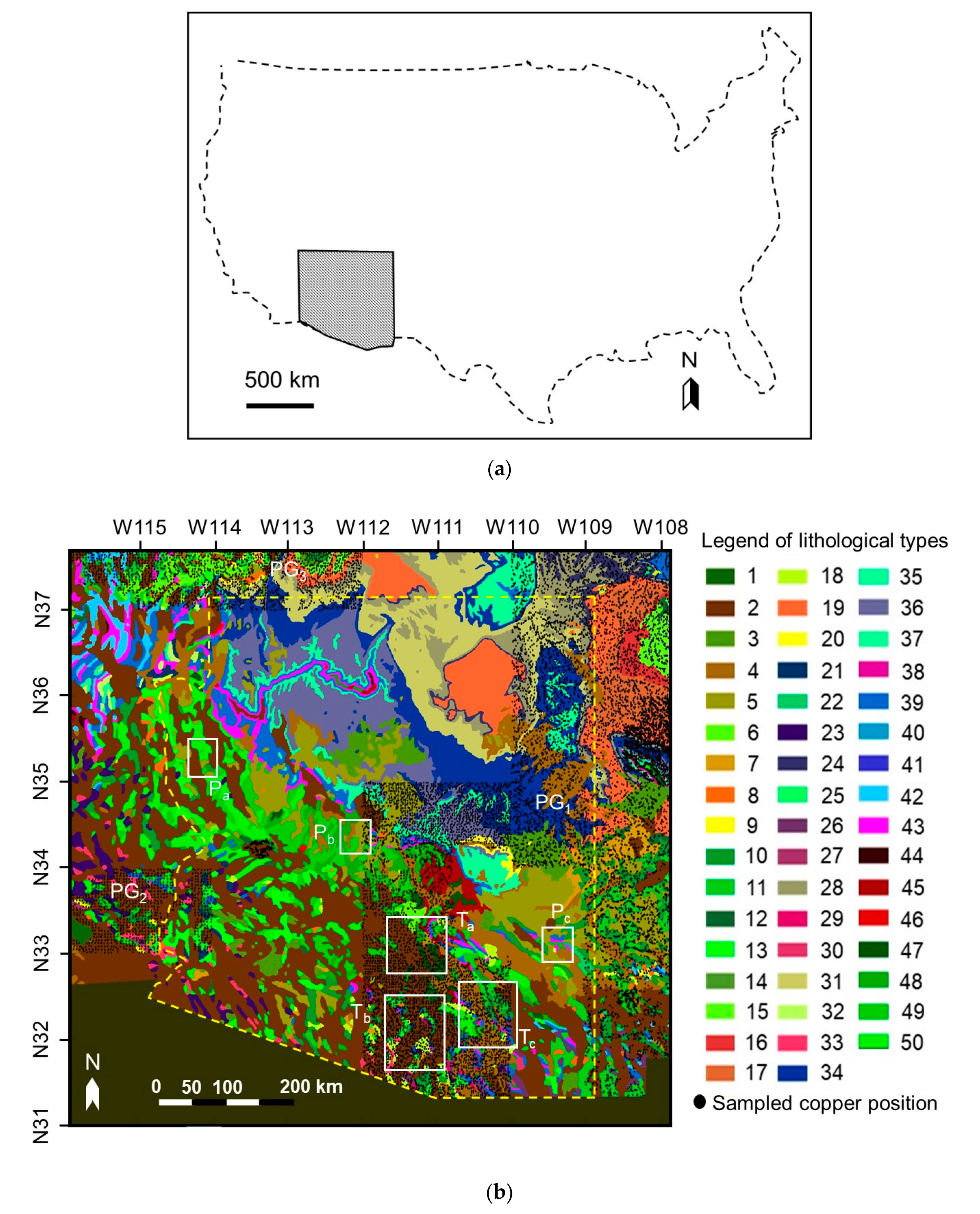
Figure 1a shows our ROI, and Figure 1b shows the boundaries of Arizona, the reference geological map, the study areas T_a, T_b, T_c, P_a, P_b, and P_c, and spatially-scattered sampled copper data points in this area. These study areas are all the detailed local areas inside the ROI. For the following validation test, T_a, T_b, T_c, P_a, P_b, and P_c were all selected to be near mining districts where mines are dense, which assured both geochemical anomalies and background content areas were included in the same map as the characteristic example model cases.

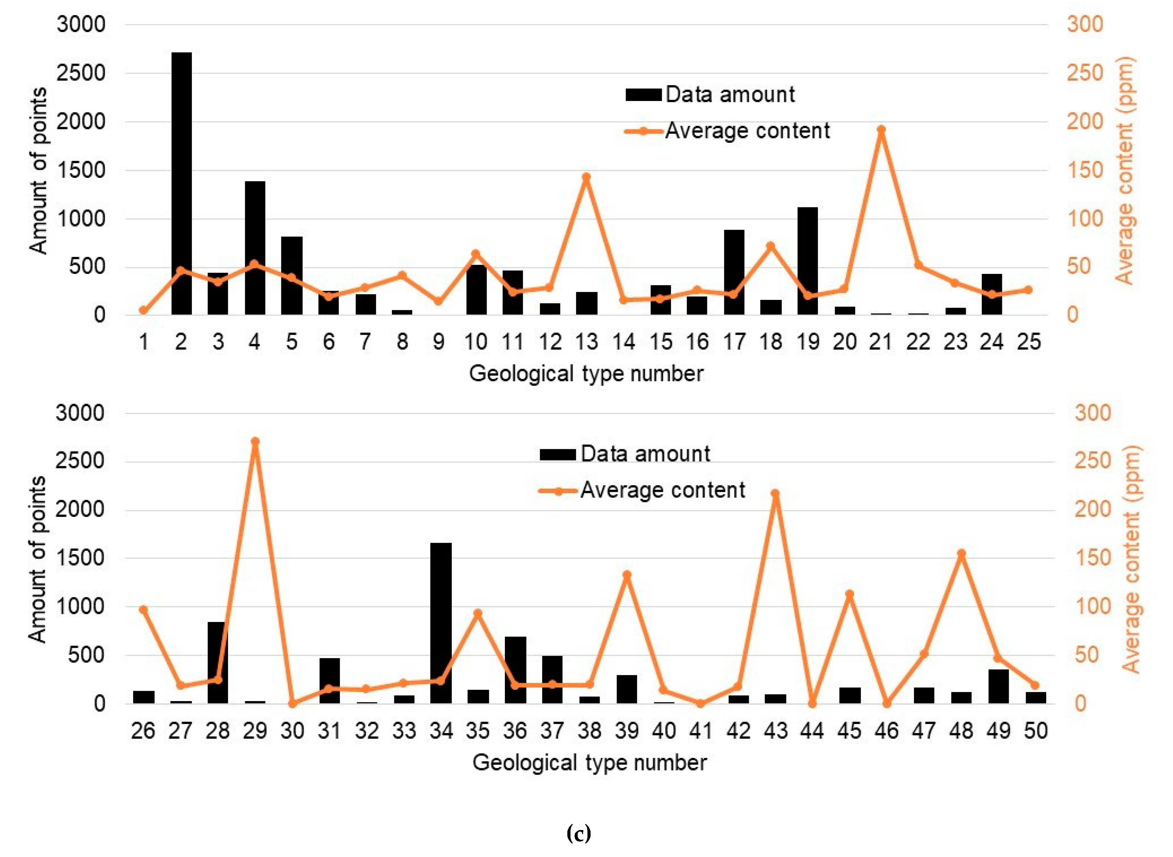
The geological map is arranged from the Geologic Map of the United States at a scale of 1:2,500,000 [22] (source: https://mrdata.usgs.gov/geology/us/kbgeology.zip). There are 50 geological/lithological (G/L) types included in the whole ROI referenced from “UNIT” in the shape file “kbge.shp”, which are numbered from 1 to 50 and are marked in different colors. A summary of G/L type names present within the ROI referenced from the “ROCK” column of the table in the shape file are listed in

Table 1. Summary of geological/lithological (G/L) types present within the study areas referenced from “ROCK” column of the table in the shape file “kbge.shp”. The G/L type numbers correspond to the numbered colors in Figure 1, Figure 2 and Figure 3.

No.	G/L Type	No.	G/L Type	No.	G/L Type	No.	G/L Type
1	Water	14	Eocene	27	Upper Mesozoic eugeosynclinal	40	Upper Paleozoic eugeosynclinal
2	Quaternary	15	Paleocene continental	28	Jurassic	41	Upper Paleozoic clastic wedge facies
3	Quaternary volcanic rocks	16	Navarro Group	29	Lower Mesozoic volcanic rocks	42	Lower Paleozoic
4	Pliocene continental	17	Taylor Group	30	Jurassic granitic rocks	43	Cambrian
5	Pliocene volcanic rocks	18	Latest Cretaceous granitic	31	Lower Jurassic and upper Triassic	44	Z sedimentary rocks
6	Pliocene felsic volcanic rocks	19	Austin and Eagle Ford Groups	32	Lower Mesozoic	45	Y sedimentary rocks
7	Miocene continental	20	Upper Cretaceous	33	Lower Mesozoic eugeosynclinal	46	Younger Y granitic rocks
8	Tertiary intrusive rocks	21	Cretaceous continental	34	Triassic	47	Older Y granitic rocks
9	Oligocene continental	22	Cretaceous volcanic rocks	35	Permian	48	X metasedimentary rocks
10	Miocene volcanic rocks	23	Cretaceous granitic rocks	36	Upper part of Leonardian Series	49	X granitic rocks
11	Miocene felsic volcanic rocks	24	Woodbine and Tuscaloosa groups	37	Lower part of Leonardian Series	50	Orthogneiss and paragneiss
12	Eocene continental	25	Fredericksburg Group	38	Wolfcampian Series continental
13	Lower Tertiary volcanic rocks	26	Lower Cretaceous	39	Upper Paleozoic

. We set the grid for the whole map (including the target variable mentioned above; the predictor variable is mentioned later) to 0.008 by 0.008 degrees in longitude and latitude, respectively (approximately 1 by 1 km in distance), resulting in an image dimension of 836 × 1003 pixels. By scattering the sampled copper data on the map in this resolution, over 50% of the map area is not covered by the sampled data, which leaves a huge blank area on the map. As a result, in our case, the sampled data compose three independent point groups (PGs) that are observed in the right side (PG₁), left median position (PG₂), and left upper position of the map (PG₃). Figure 1c shows the statistics of sampled copper data amounts and average contents of all sampled copper data in each lithological type area.

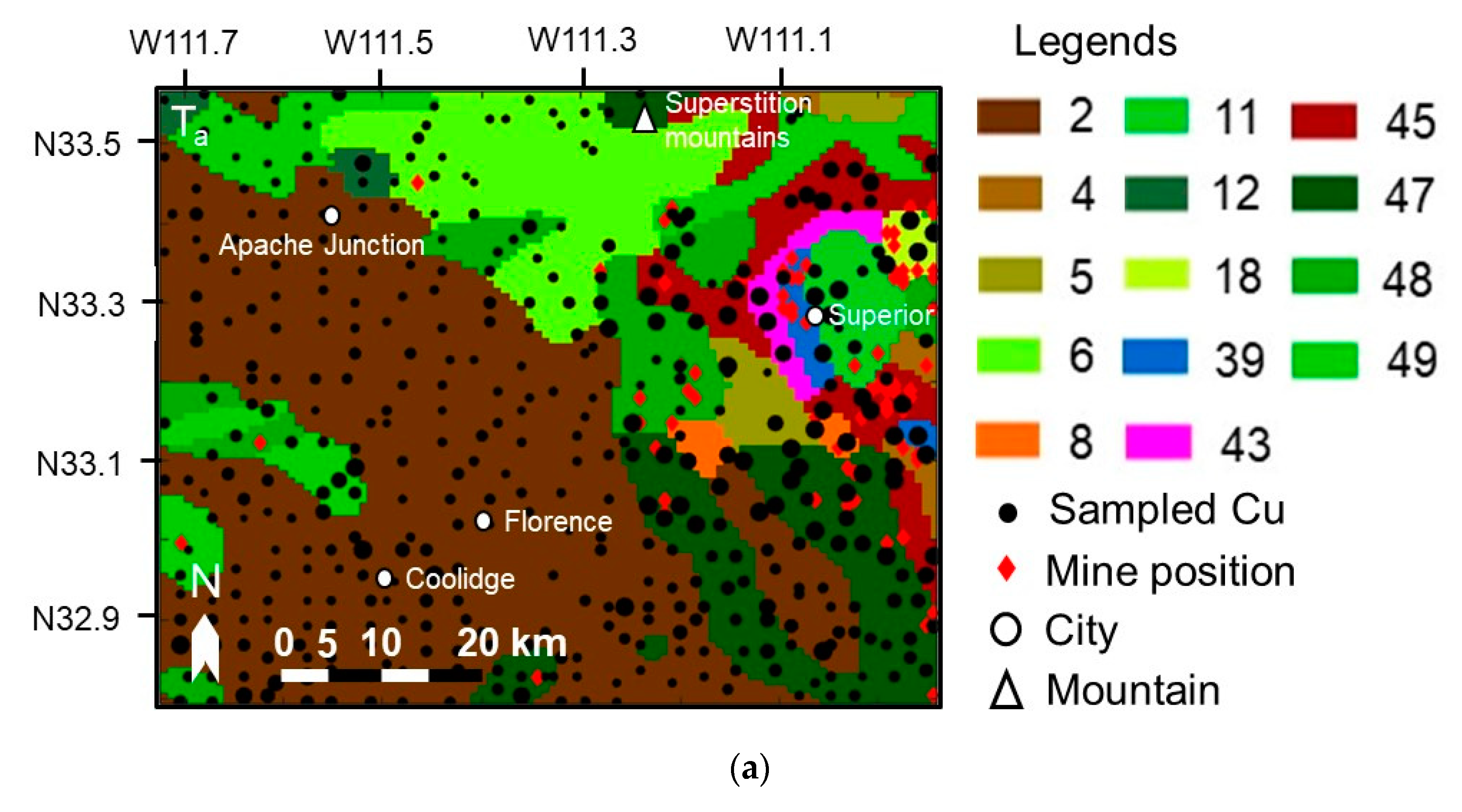
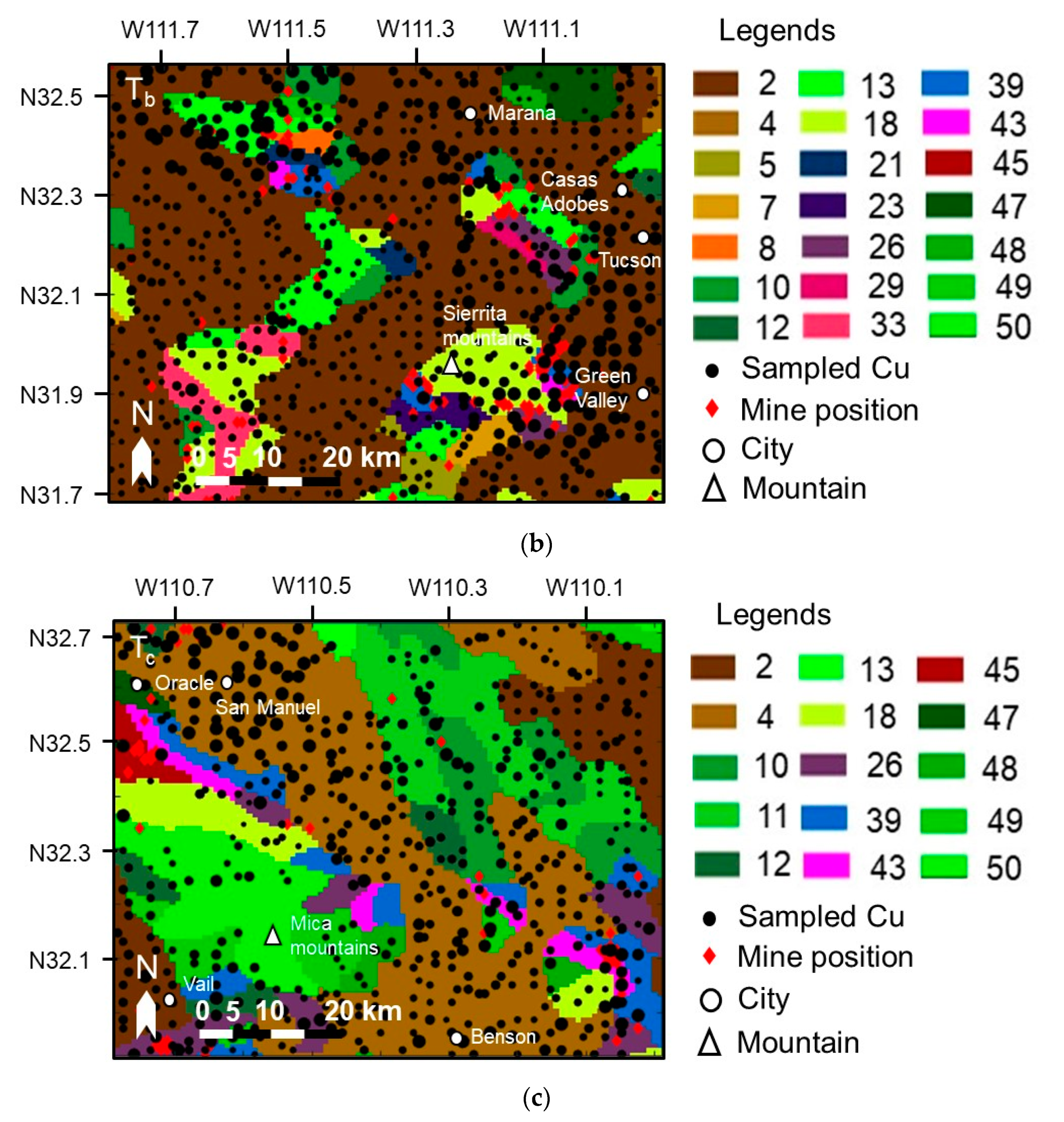
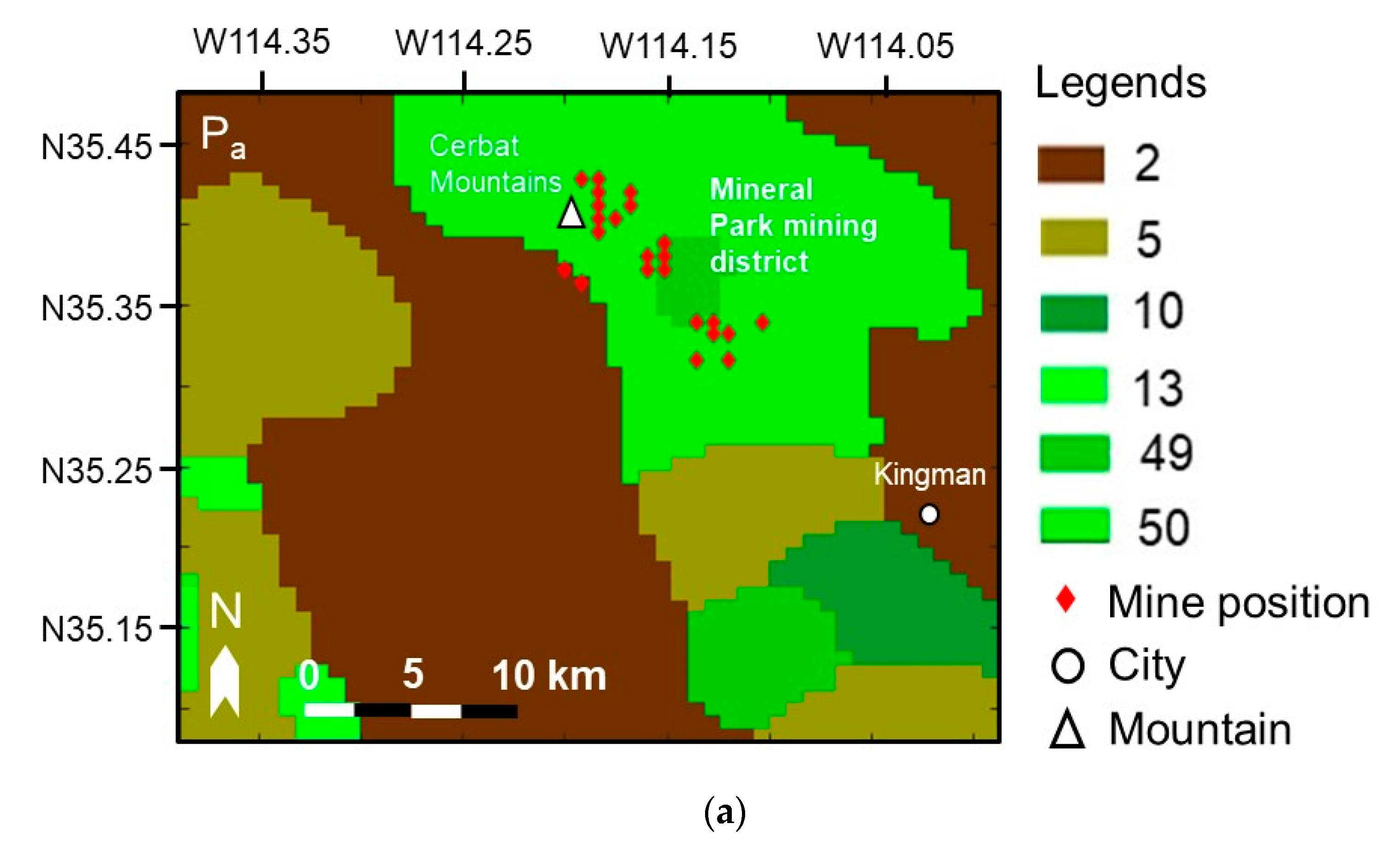
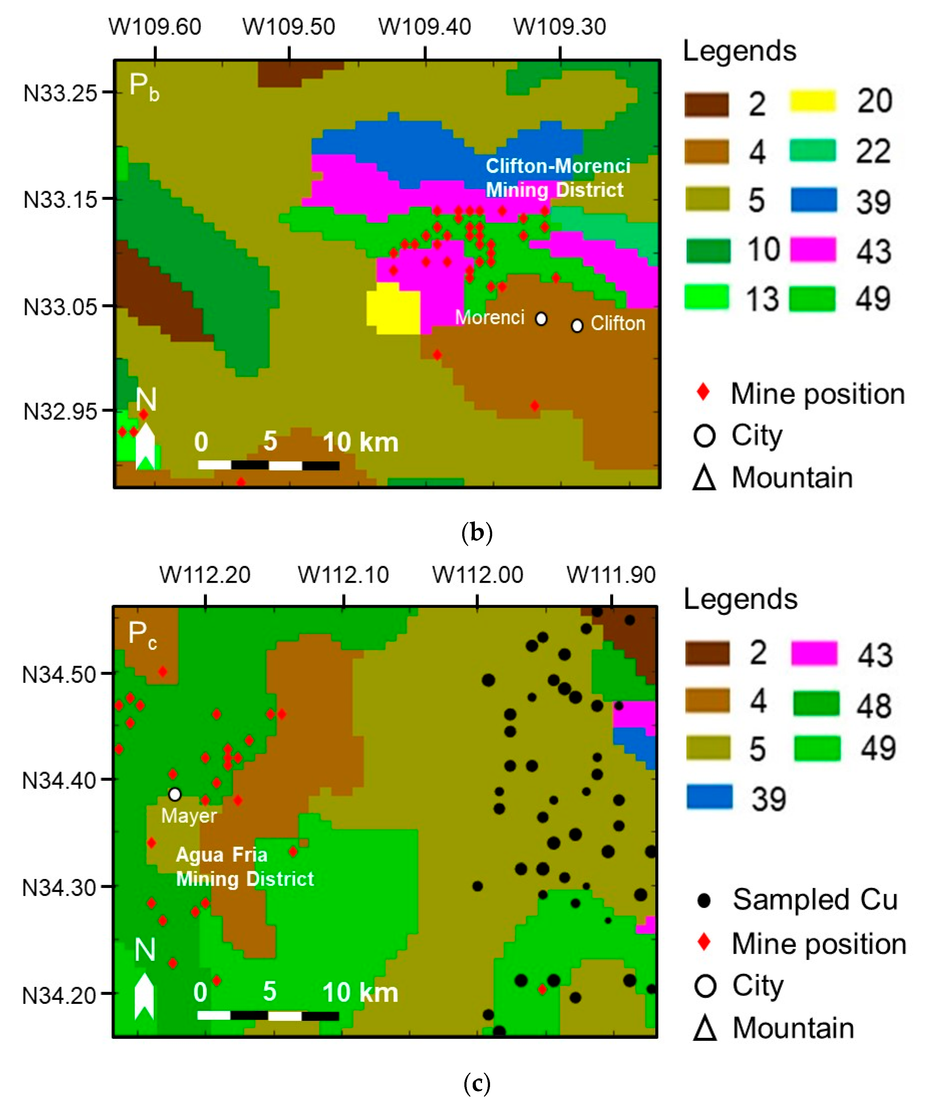
The details of T_a, T_b, T_c, P_a, P_b, and P_c are shown in Figure 2 and Figure 3, and

Table 2. Detailed information of T_a, T_b, T_c, P_a, P_b, and P_c.

Area	Range	Resolution
Ta	(W111.7200, N33.5638)–(W110.9440, N32.7958)	110 × 110
Tb	(W111.7840, N32.5558)–(W110.9120, N31.6838)	110 × 110
Tc	(W110.7840, N32.7158)–(W109.9920, N31.9238)	110 × 110
Pa	(W114.3840, N35.4758)–(W113.9840, N35.0758)	50 × 50
Pb	(W109.6240, N33.2758)–(W109.2240, N32.8758)	50 × 50
Pc	(W112.2640, N34.5558)–(W111.8640, N34.1558)	50 × 50

. The sampled copper data are plotted by black circles on the reference geological map, with the size of a black circle proportional to the copper content. The coordinates of copper mines in Arizona referenced from the Mineral Resources Data System of the United States Geological Survey (USGS) [23,24] are also plotted by red diamonds (source: https://mrdata.usgs.gov/mrds/output/mrds-fUS04.zip). Only those copper mines whose “dev_stat” in the shape files are labeled “Producer” or “Past Producer” are marked. A number of important landmarks such as cities and mountains are also marked on the map to show as references of the approximate positions. A detailed introduction of the study areas is summarized in the supplementary material (Table S1).

2.2. Predictor Variables–High-Resolution Remote Sensing Data

All of the available remote sensing data including that from the advanced spaceborne thermal emission and reflection radiometer (ASTER) data, digital elevation model (DEM), and geophysics (geomagnetic) data [25] are used to create an ML model to make predictions. Matlab (Mathworks, Natick, USA) is used for all of the data processing and calculations here and in the sections below.

All the ASTER data are extracted from “ASTER Level 1T” and DEM data are extracted from “ASTER Global Digital Elevation Model” in the USGS’s EarthExplorer search engine, respectively (source: https://lpdaac.usgs.gov/data_access/data_pool, courtesy of the NASA Land Processes Distributed Active Archive Center (LP DAAC), USGS/Earth Resources Observation and Science (EROS) Center, Sioux Falls, South Dakota). The ASTER data are part of the ASTER Level 1T group, and the search filter is set as follows: Cloud cover is “less than 10%”; correction achieved is “all”; and SWIR, TIR, and VNIR1 modes are all “on”. Geomagnetic data are obtained from magnetic anomaly maps and data for North America [25] (source: https://mrdata.usgs.gov/magnetic/USmag_origmrg.zip). The geomagnetic data are international geomagnetic reference field (IGRF) residual signals taken from a height of 305 m, the precision of which is approximately 1–10 nT.

One shot from an ASTER satellite can only cover 60 × 60 km, and a DEM can only cover an area approximately 100 × 100 km on Earth; therefore, to cover the whole ROI in this research, we retrieved a total of 637 ASTER images and 160 DEM images from the data pool and created a composite of all the images in accordance with their longitude and latitude to create a wide-range map. The detail of the source of ASTER and DEM data are listed in Tables S2–S4 of the supplementary document. All the ASTER band data are extracted from the “.hdf” file by the “hdftool” of Matlab, and DEM data are obtained by translating the “.tiff” DEM image to a digital number.

The resolutions of these predictors are all different (15 of ASTER visible and near-infrared (VNIR) band data, 30 of ASTER short wave infrared (SWIR) band data, 90 of ASTER thermal band data, 30 of DEM data, and 5 km of geomagnetic data). The VNIR and SWIR data and DEM data are 8-bit, and the thermal data are 12-bit. The geomagnetic data are processed into four types: Analytic signal-processed geomagnetic data, reduction to pole-processed geomagnetic data, residual IGRF- and vertical first derivative-processed geomagnetic data. ASTER and DEM predictor variables and their derivatives are reprocessed from their original data grid to a regular 1-km grid to be studied using bicubic interpolation and geomagnetic predictor variables are reprocessed using the nearest interpolation, i.e., 5 × 5 pixels in a 1-km grid will be the same value.

The derivatives of ASTER as predictors include all the commonly used ASTER band ratios and their combinations that are reported as a significant lithological index for geological mapping [26,27]. For example, the carbonate index (No. 41 predictor in

Table 3. Predictor variables used in this research.

Group	No.	Predictor	Predictor Description
Geo-magnetic	1	Mag_AS	Analytic signal processed geomagnetic data
	2	Mag_RTP	Reduction to pole processed geomagnetic data
	3	Mag_TMI	The residual of international geomagnetic reference field (IGRF)
	4	Mag_VD	Vertical first derivative processed geomagnetic data
DEM	5	Altitude	The altitude of the Earth surface, from 0–2500 m
	6	Slope	The elevation of the Earth surface
ASTER Band	7	Band_1	The ASTER band 1 sensor data
	8	Band_2	The ASTER band 2 sensor data
	9	Band_3N	The ASTER band 3N sensor data
	10	Band_4	The ASTER band 4 sensor data
	11	Band_5	The ASTER band 5 sensor data
	12	Band_6	The ASTER band 6 sensor data
	13	Band_7	The ASTER band 7 sensor data
	14	Band_8	The ASTER band 8 sensor data
	15	Band_9	The ASTER band 9 sensor data
	16	Band_10	The ASTER band 10 sensor data
	17	Band_11	The ASTER band 11 sensor data
	18	Band_12	The ASTER band 12 sensor data
	19	Band_13	The ASTER band 13 sensor data
	20	Band_14	The ASTER band 14 sensor data
	21	Band_1_R	The reverse of 7
	22	Band_2_R	The reverse of 8
	23	Band_3_R	The reverse of 9
	24	Band_4_R	The reverse of 10
	25	Band_5_R	The reverse of 11
	26	Band_6_R	The reverse of 12
	27	Band_7_R	The reverse of 13
	28	Band_8_R	The reverse of 14
	29	Band_9_R	The reverse of 15
	30	Band_10_R	The reverse of 16
	31	Band_11_R	The reverse of 17
	32	Band_12_R	The reverse of 18
	33	Band_13_R	The reverse of 19
	34	Band_14_R	The reverse of 20
ASTER lithological index	35	R_Ferric_iron	Feature index of Fe3+, =8/7
	36	R_Ferrous_iron	Feature index of Fe2+, =11/9 + 7/8
	37	R_Laterite	Feature index of laterite, =10/11
	38	R_Gosan	Feature index of gosan, =10/8
	39	R_Ferrous_Silica	Feature index of ferrous silicates, mainly Fe oxide Cu-Au alteration, =11/10
	40	R_Ferric_oxides	Feature index of ferric oxides, =10/9
	41	R_Carbonate	Feature index of carbonate/chlorite/epidote, =(13 + 15)/14
	42	R_Epidote	Feature index of epidote/chlorite/amphibole, =(12 + 15)/(13 + 14)
	43	R_MgOH	Feature index of Amphibole/MgOH, =(12 + 15)/14
	44	R_Amphibole	Feature index of amphibole, =12/14
	45	R_Carbonate2	Feature index of carbonate, =19/20
	46	R_Dolomite	Feature index of dolomite, =(12 + 14)/13
	47	R_Sericite	Feature index of sericite/muscovite/illite/smectite, =(11 + 13)/12
	48	R_Alunite	Feature index of alunite/kaolinite/pyrophyllite, =(10 + 1 2)/11
	49	R_phengitic	Feature index of phengitic, =11/12
	50	R_Muscovite	Feature index of muscovite, =13/12
	51	R_Kaolinite	Feature index of kaolinite, =13/11
	52	R_Quartz	Feature index of quartz rich rocks, =20/18
	53	R_Basic_deg	Feature index of basic degree index of SiO2, =18/19
	54	R_SiO2	Feature index of SiO2, =19/18
	55	R_Siliceous_rock	Feature index of siliceous rocks, =172/(16 × 18)
	56	R_Silica1	Feature index of the first pattern of silica, =17/16
	57	R_Silica2	Feature index of the second pattern of silica, =17/18
	58	R_Silica3	Feature index of the third pattern of silica, =19/16
	59	R_Vegetation	Feature index of vegetation, =9/8
	60	R_Clay	Feature index of clay, =(11 × 13)/122
	61	R_NDVI	Feature index of NDVI, =(9 − 8)/(9 + 8)
Coordinates	62	x	Longitude
	63	y	Latitude

) map is acquired by calculating the image of Band 13, 14, 15 pixel-by-pixel. A total of 63 predictor variables used in this research are listed in Table 3. The predictors are categorized into five groups: Geomagnetic, DEM, ASTER band, ASTER lithological index, and Coordinates.

2.3. Spatial Autocorrelation-Based Mixture Interpolation Algorithm

2.3.1. The Process of the SABAMIN Algorithm

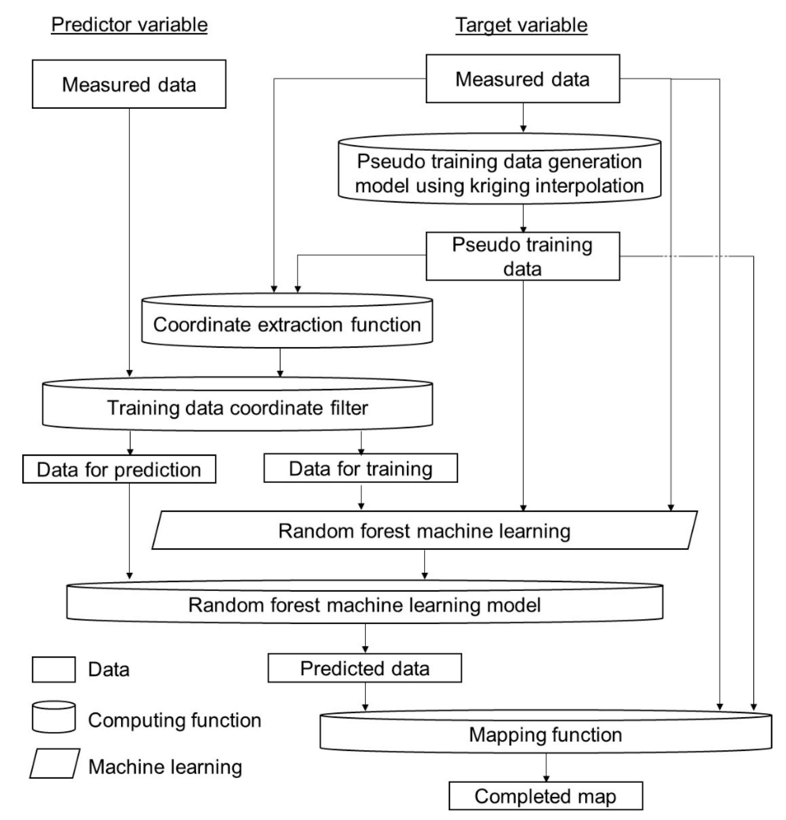
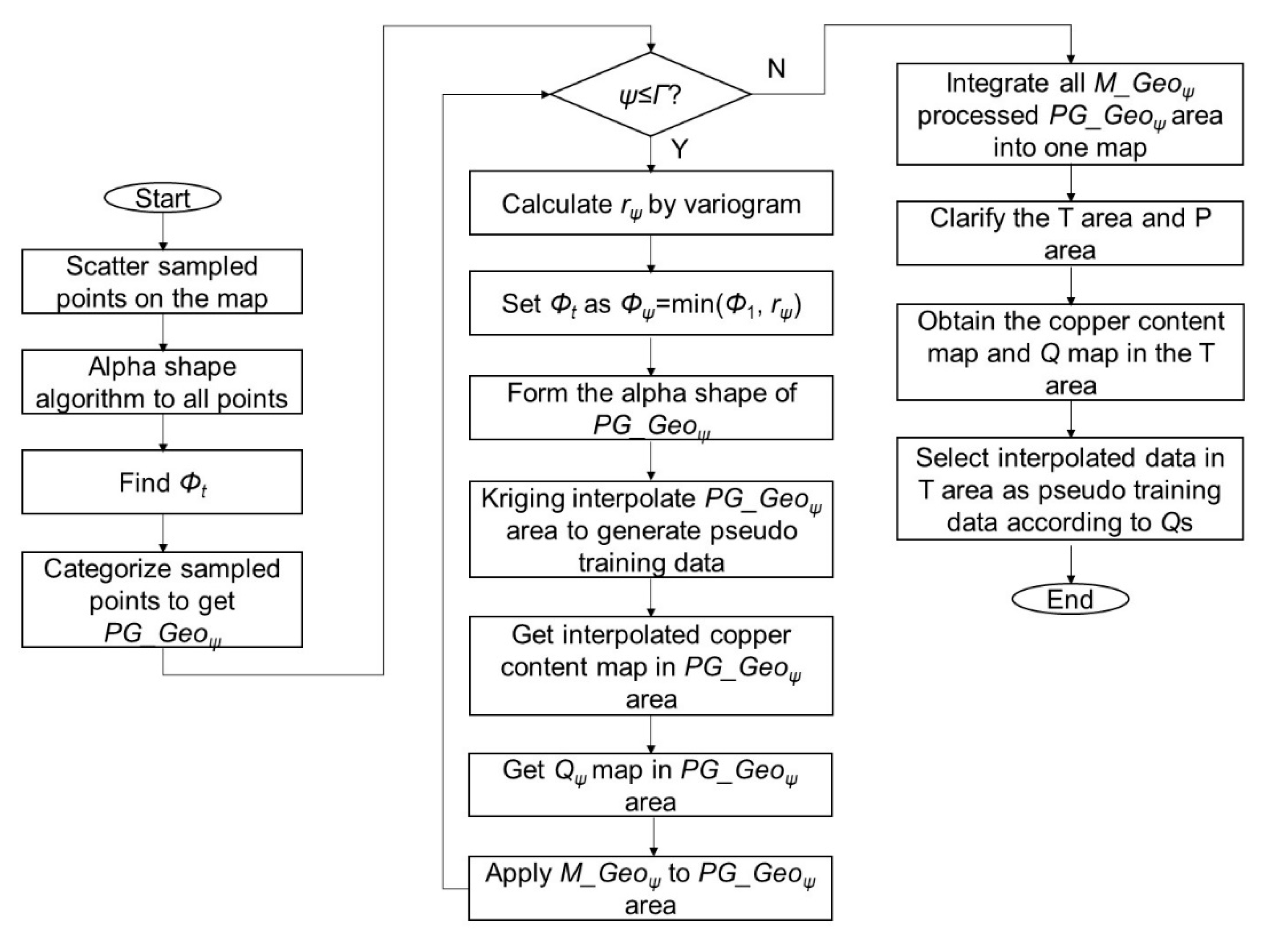
Figure 4 shows the flow chart of the SABAMIN algorithm. First of all, the measured target variable data are input into the pseudo training data generation model by using kriging interpolation, and then the pseudo training data are generated. Both are applied for composing of training datasets. Meanwhile, both are input into a coordinate extraction function, then the coordinates of training datasets are extracted to construct a coordinate filter for selecting predictor variable data in correspondent pixel from the whole ROI. Furthermore, by this coordinate filter, the ROI is divided into two areas: “Areas for training” (T areas) and the remaining blank areas as “areas waiting to be predicted” (P areas), and the predictor variable data is divided into “data for training” and “data for prediction”, respectively. Through RF learning, a prediction model is generated and by inputting data for prediction into this model, the target variable data in P area are generated. Finally, using a mapping function, the measured data, pseudo training data, and predicted data are merged together to complete a whole-pixel map of the ROI. This is a process of mixing univariate interpolation and multivariate prediction; thus, we named our new algorithm spatial autocorrelation-based mixture interpolation.

2.3.2. How to Generate Pseudo Training Data in Our Case

The generation of pseudo training data is a crucial part of algorithm. It is important that pseudo training data are reliable. However, in our case, there are problems that need to be solved. Below, we introduce how to generate reliable pseudo training data in our case.

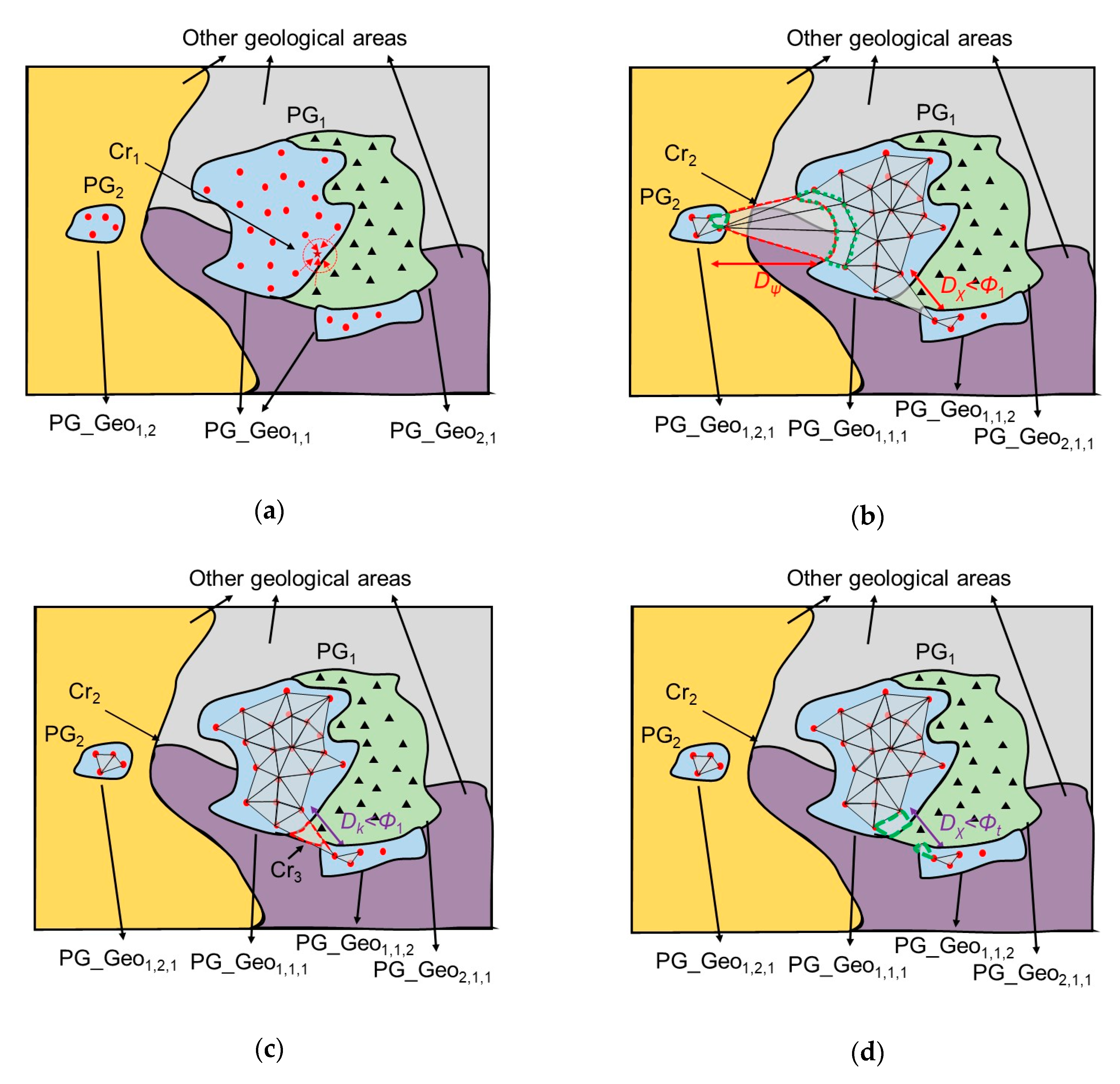
Figure 5 shows a conceptual drawing explaining these problems. As mentioned before, kriging interpolation is reliable in a range of r. However, mineral contents have been reported to be highly correlated with lithological features [28,29,30]; thus, it is considered that the spatial autocorrelations within points of different geological areas are different and the correlation between two different areas is lower. Due to geological discriminations that exist at the area border, different G/L types are considered to have different r. If the interpolation model is produced under the condition that a single r is set by fusing all sampled points in the study area, distribution crosstalk Cr₁ (Figure 5a) will occur in the regions near the borders of different geological areas because the neighboring sampled points inside the range of r may come from different geological areas. Therefore, the pseudo training data in Cr₁, which do not make sense in geoscience, are too unreliable to be used. To avoid Cr₁, it is necessary to determine reliable spatial sections that enable reliable pseudo training data points inside them. Therefore, kriging interpolation must be processed in each geological area independently.

Sampled points are categorized into different point groups in accordance with G/L types, which are defined as PG_Geo_ψ ψ = 1, …, Γ, where Γ is the total number of G/L types in the study area, and they need to be separated from each other spatially. Creating an envelope of the PGs enables them to be separated from each other. To achieve this, a computational geometry strategy is applied here.

Observing the distribution shape of PG_Geo_ψ domains, they are not usually geometrically convex, but always contain multiple concave parts. The alpha shape [31], an algorithm capable of generating an optimized envelope in this case, was chosen for an automatic enveloping generation process. An alpha shape is a family of piecewise linear simple curves in the Euclidean plane associated with the shape of a finite set of points. The PG is split into multiple triangles by Delaunay triangulation [32], wherein each edge or triangle may be associated with a characteristic radius; the radius Φ of the smallest empty circle containing an edge or triangle. After the alpha shape has been formed, a closed spatial section is partitioned by the edge of the shape, and the points inside the shape that can be judged by a point-in-polygon algorithm [33] can be considered reliable to enable all vacant pixels to be interpolated inside the shape.

By applying the alpha shape algorithm without setting Φ, Delaunay triangles (DTs) among the points are formed to connect all points in the PGs to each other. As shown in Figure 1, there are a number of G/L types that are included in PG₁, PG₂, and PG₃. The DTs cover the points in the intermediate blank parts even though they belong to different geological areas. This generates crosstalk Cr₂ (Figure 5b), which covers those blank areas. Compared with the relatively smaller DTs inside PG₁ or PG₂, the size of the DTs across two PGs are big and the distances from their internal points to most neighboring sampled points are far. Therefore, the reliability of the estimated points inside these big DTs is low for pseudo training data. To avoid Cr₂, it is necessary to correctly select the threshold of Φ, to divide PG_Geo_i into PG_Geo_ψ,ω, where PG_Geo_ψ,ω belongs to PG_ω, ω = 1, 2, 3, and then to obtain the optimized shape of the envelope of each PG_Geo_ψ,ω. Therefore, for all data points, a threshold Φ_t that forms three independent parts in the alpha shape process is needed to be specified first.

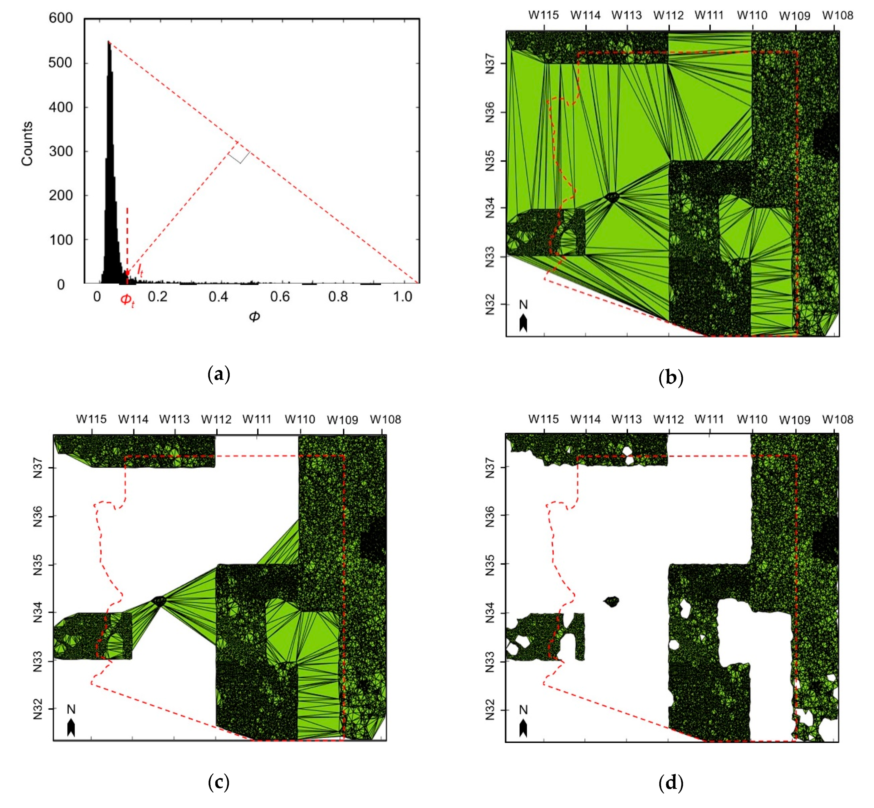
When the points are concentrated at different places on the plane that consist of different groups, for all points, the value of Φ within the PGs is small but the amount of small Φ is large, while the value of Φ between the PGs is large but the amount of such large Φ is small. If the threshold of Φ is set to cover most of Φ within the PGs and discard the remaining ones, the DTs between the PGs will disappear and the envelope of each PG will be generated. To achieve this, determining the turning point between the histogram of Φ from the maximum position to infinite is considered effective to find Φ_t, which can be actualized by, for example, a triangle thresholding algorithm [34]. The histogram of Φ of all the datasets used in this research is shown in Figure 6a. According to the triangle thresholding algorithm, Φ_t is specified by the following process: Connect the peak value and the value at infinity by a line, search for the furthest point I_t from the line on the histogram envelope, and specify the corresponding Φ of I_t. The alpha shapes are calculated under the conditions of setting Φ to infinity (Figure 6b), Φ_t < Φ < +∞ (Figure 6c), and Φ = Φ_t (Figure 6d). The calculated Φ_t is 0.0848 degree in longitude and latitude, defined as Φ₁ here, and the length is approximately 10 pixels in our case. For each PG_Geo_ψ, it is divided into PG_Geo_ψ,ω.

In a number of cases, it is clear that there are multiple PGs, PG_Geo_ψ,ω,χ, χ = 1, … , Ω, not connecting with each other that belong to the same PG_Geo_ψ,ω. The distances D_χ between these areas may be smaller than Φ_t, which indicates that this alpha shape algorithm is not effective to divide all observed independent PGs, leaving crosstalk parts with adhering geological area Cr₃ (Figure 5c). Here, Ω is the total number of these independent PGs in PG_Geo_ψ,ω. We first directly performed kriging interpolation while ignoring the effect of Cr₃. Then, to handle Cr₃, G/L type labels were plotted for every pixel on the map in accordance with the data, as shown in Figure 1, to create image masks, M_Geo_ψ for excluding those points not covered by M_Geo_ψ. After the filtering process, Cr₃ was also eliminated, and kriging interpolation on a single geological area could be successfully performed.

It should be noted that all vacant pixels in a DT must correlate with at least three neighboring points (the apexes of the correspondent DTs and three points determine a plane) in accordance with kriging interpolation, where Φ of a DT must be smaller than r_ψ. If not, several vacant pixels located at the center of a DT will not be subject to kriging interpolation. Therefore, to form an alpha shape of each PG_Geo_ψ, Φ_t should be set as Φ_ψ = min(Φ₁, r_ψ).

If we did not apply M_Geo_ψ after the DTs were formed and before Φ_t was specified, a number of badly estimated pseudo training data points would be included, even though part of the process could be omitted. In cases when the distance between PG₁ and PG₂ and D_ψ, were smaller than r₁ (the example in Figure 5b), vacant pixels in DTs included in Cr₂ would be also interpolated. Even if Cr₂ was eliminated by M_Geo_ψ cropping, those badly estimated points (inside the green dashed line surrounding the region in Figure 5b) remained in the candidate training region. If we followed the process mentioned above, although there were still a number of less reliable areas remaining, the surface would be greatly suppressed (green dashed line surrounding the region in Figure 5d).

According to Equation (3), an inverse computation of an (N × N) matrix is included in kriging interpolation. To ensure the computation speed of the computer, we compromised by generating pseudo training data using only three neighboring points. Thanks to the alpha shape algorithm, interpolation was processed independently in a single DT unit by using the apexes’ values.

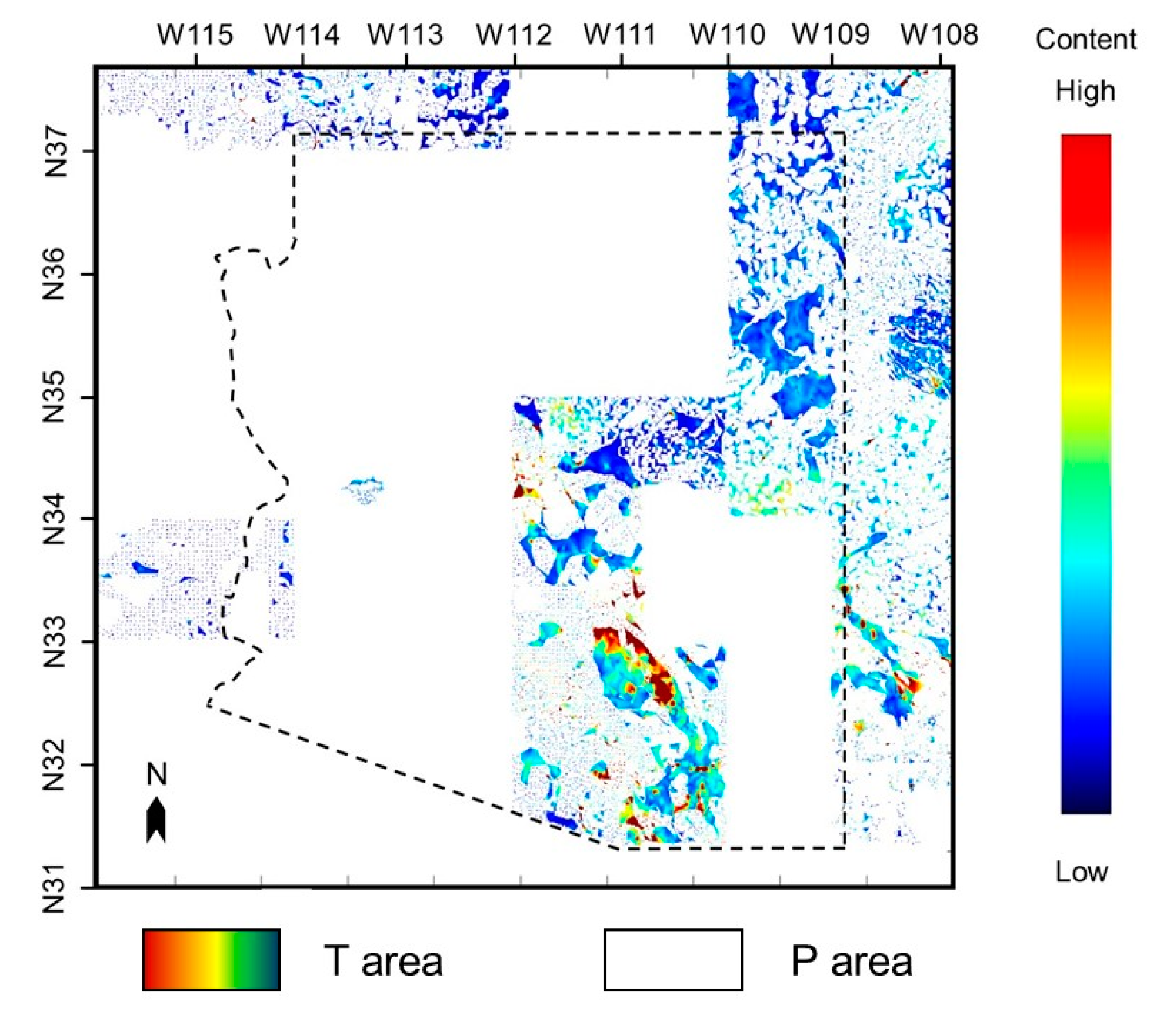
The result after kriging interpolation in all PG_Geo_ψ,ω is shown in Figure 7. Here, T areas is the colored area and the remaining white areas are P areas, respectively. However, not every interpolated data point in the T areas can be treated as pseudo training data. As mentioned above, because the further the distance from the interpolated points to the measured points is, the lower the reliability of the interpolated value. A large amount of relatively low reliability data will reduce the reliability of the constructed prediction model. To ensure reliability, a penalty on selection probability Q going into the training dataset is given to each data point. The selection probability is proportional to the minimum distance b_min from the candidate interpolated point A_j in a DT to the three apexes’ measured data S_α, where α = 1, 2, 3. b_min can be expressed by Equation (15), and Q can be expressed by Equation (16):

$$b_{min}=\underset{A_j\in D{T}_{\epsilon }}{\min }\Vert A_j-S_{\alpha }\Vert \alpha =1,2,3$$

(15)

$$Q_{\psi }=\{\begin{array}{c}{\left(\frac{{\Phi }_{\psi }-b_{min}}{{\Phi }_{\psi }}\right)}^2, b_{min,\psi }<{\Phi }_{\psi }\hfill \\ 0, b_{min,\psi }\ge {\Phi }_{\psi } or A_j\notin D{T}_{\epsilon }\hfill \end{array}$$

(16)

The equations indicate that the apexes (b_min = 0), which are also the measured points, will be absolutely selected, and the points outside these DT areas will not be selected. Whether the interpolated data in the T areas will be selected as pseudo training data is determined by their Qs. Finally, the flow chart of pseudo training datasets in our case is shown in Figure 8.

2.4. Algorithm Validity Test

The validity test of the proposed algorithm includes four parts: (i) Cross-validation of measured data, (ii) blind test in T areas, (iii) temporal stability test in P areas and (iv) predictor importance test. The validity of the constructed model by SABAMIN is compared with that by only RF, which does not merge the spatial autocorrelation into ML.

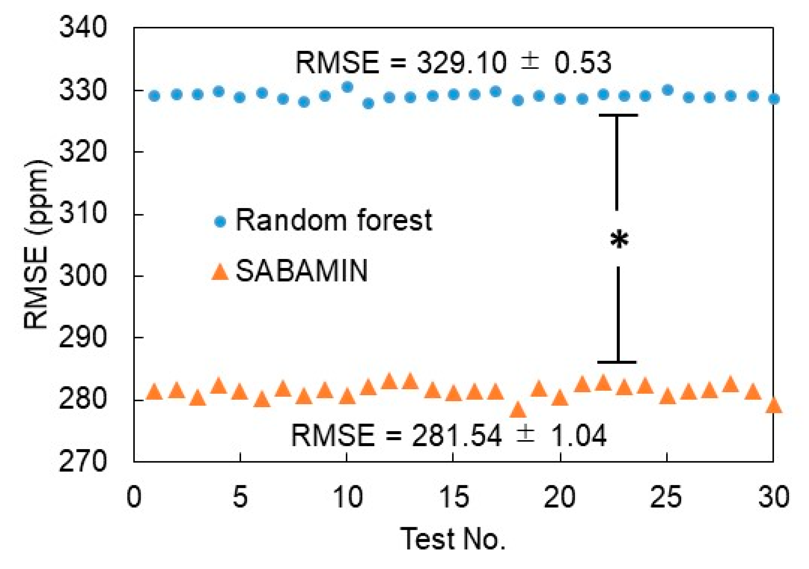
First, the cross-validation test of measured data was done to test the precision of the constructed prediction model. The measured data were the most reliable values in the datasets: If the prediction values in the cross-validation were near to the real value, the precision of the model was good. The precision was evaluated by the root mean squared error (RMSE) between the predicted value and real value through 10-fold cross-validation. In the cross-validation, all training datasets were randomly divided into 10 groups, then 9 groups were selected for training, and the remaining 1 group was selected for validation. To compare the two models fairly, only real and predicted values in actual sampled points were picked up for calculating RMSE.

Second, blind testing in T areas was done to test the accuracy of the T area. If the accuracy is good, spatial continuity should still be reserved well by the model, that is, the predicted map should have a similar distribution to the original one. To confirm this, a blind test was conducted in the T area. During one test, data in the selected area were excluded from the training data, and the remaining data were used to construct the prediction model. The distribution of the excluded area was then predicted by the constructed model and compared with the real distribution. Only data from actual sampled points were selected in the evaluation. The RMSE and Pearson product–moment correlation coefficient (R_t) were used to evaluate the similarity between the predicted and real distributions. The study areas, T_a, T_b, and T_c were selected for three different blind tests. To confirm whether the model could handle the prediction of geochemical anomalies, zones around the mining districts were considered as candidate areas for the test.

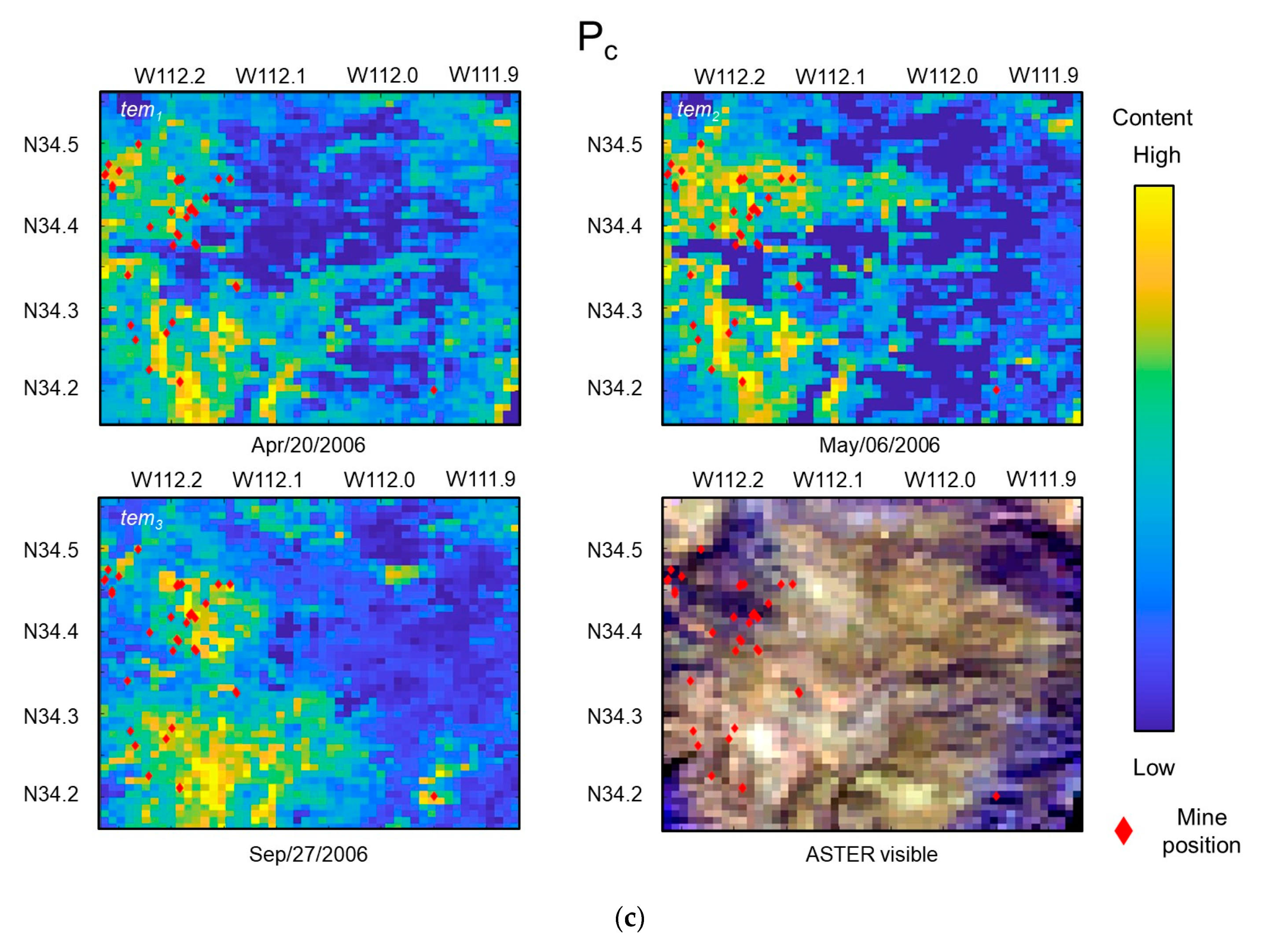
Third, the temporal stability test in P areas was done to test the accuracy of P area. Since there were no geochemical data in a P area, it was difficult to validate our algorithm by comparing the predicted value with the real value. We considered that, as shown in Figure 2, the copper content in the rocks around a copper mine should be high, so checking whether high copper content areas were located around copper mining districts was considered a compromised method for the reliability test. Furthermore, it was considered that if the reliability of the algorithm was high, the similarity between the different predicted distributions using ASTER images of different time series should be high. In all cases, the predicted high content areas should be located around the copper mines. The similarity of all pairs of predicted maps in different time series were calculated, and an average similarity of them was used to compare the reliabilities of SABAMIN and RF. The Pearson product–moment correlation coefficient (R_p) was used to evaluate the similarity. Three study areas, P_a, P_b, and P_c in the P areas, which are all located around copper mining districts, were selected for these tests.

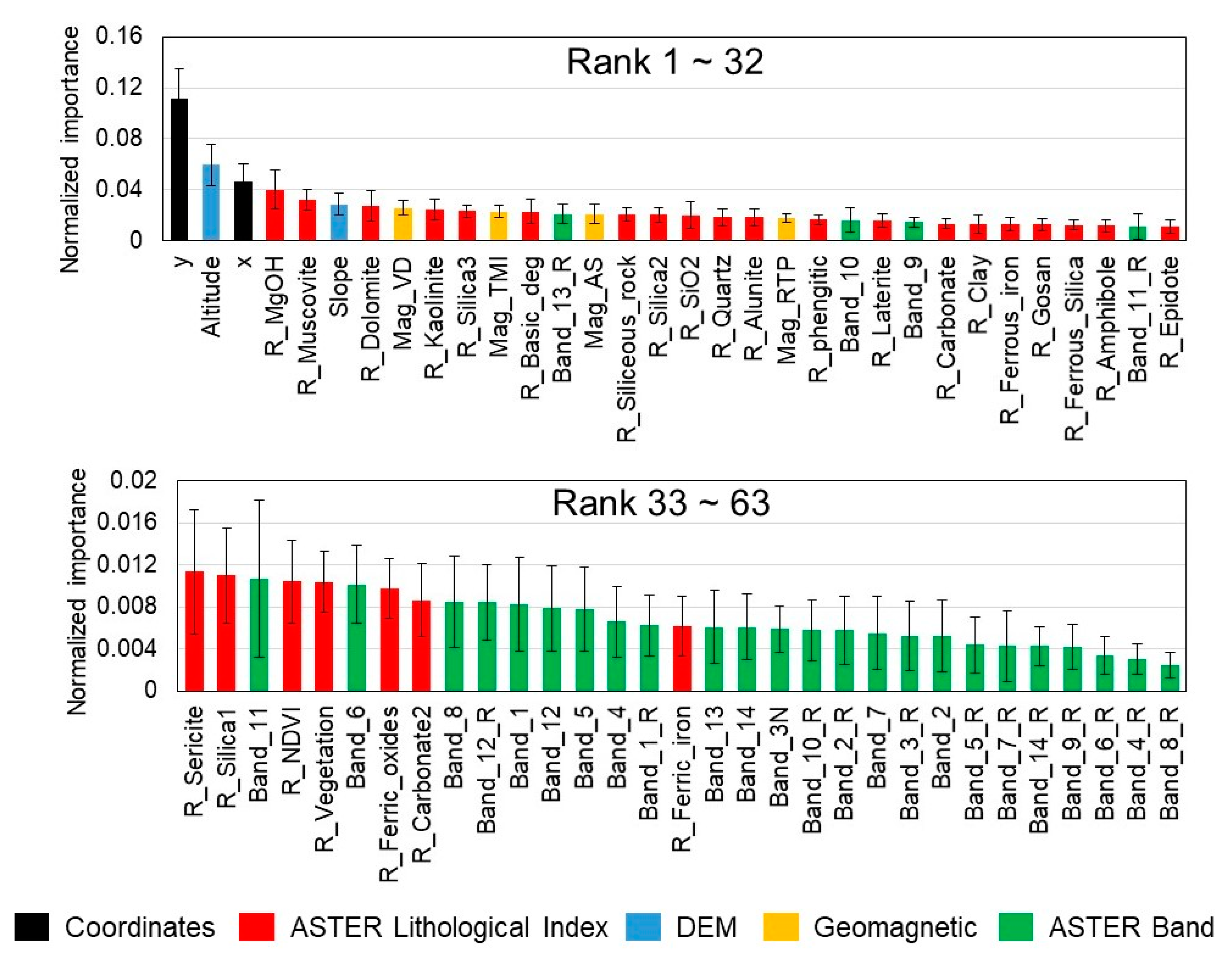
Fourth, the predictor importance of different groups ImG was also calculated to check whether the constructed model was geologically reasonable and to determine whether the constructed model was biased to any predictor. If the predictors in the high importance ranking were the factors which were already known to be highly correlative to copper content-based conventional geological knowledge, for example, high copper contents tend to distribute around copper mine restricts which are always located in the mountain, and if the topographic factors were in the high importance ranking, the model was considered geologically reasonable. To check predictor bias, first, the normalized importance of all predictor variables Im_w, w = 1, …, 63, were calculated by the RF, and then, in accordance with Table 2, they were allotted to different groups ImG_mag, ImG_dem, ImG_band, ImG_lith, ImG_cor, which represent geomagnetic variables, DEM variables, ASTER band variables, ASTER lithological index variables, and coordinate variables groups, respectively. ImG was obtained by summing all of the members’ importance in the group. As a good selection of predictor variable, the constructed model should not be biased to any predictor.

Random processes are seen in both the RF and SABAMIN. In the RF, the random creating node of trees by randomly selecting training variables induces a random process. That random selection process for creating a prediction model generates a random factor in SABAMIN. As a result, the calculated RMSE, R_t, and R_p are not constant values. Therefore, their means and standard deviations are calculated from 30 repeated tests and used for comparison in tests (i) and (ii), and the average predicted distributions of the repeated tests are used in test (iii). Moreover, the mean and standard deviation of the predictor’s importance are calculated from 30 repeated tests. Two-sided t-tests are used to examine the differences between groups. For all analyses, the statistical significance is set to p < 0.05.

3. Results

3.1. Cross-Validation Test of Measured Data

The 10-fold cross-validation results of the RF and SABAMIN are shown together in Figure 9. The test was repeated 30 times. As a result, the RMSE of the RF and SABAMIN was 329.10 ± 0.53 and 281.54 ± 1.04 ppm, respectively. A significant difference is seen between the precision test results, which means the constructed prediction model by SABAMIN was more accurate than that of RF.

3.2. Blind Test in T Area

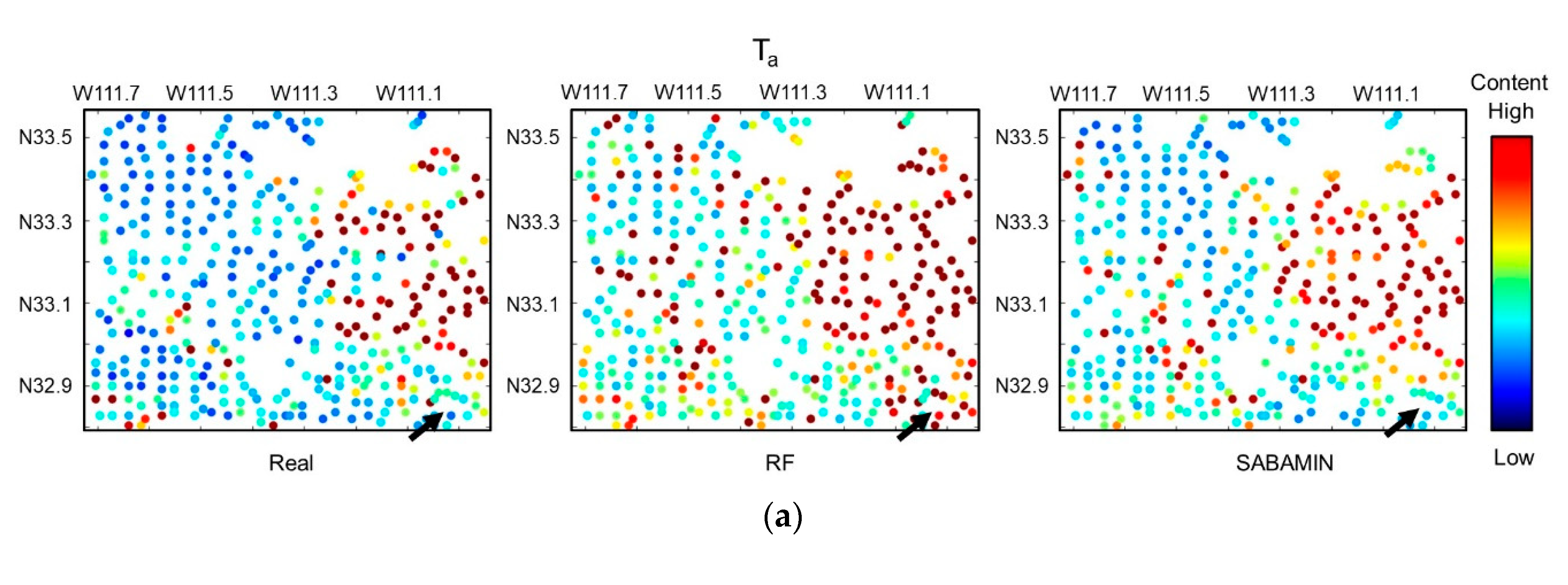
The blind test results of T_a, T_b, and T_c are shown in Figure 10a–c, respectively. In each panel, the real distribution, RF-predicted distribution, and SABAMIN-predicted distribution are compared. The results of the RMSE and R_t are shown in

Table 4. Root mean squared error (RMSE) and R_t results of the RF and SABAMIN. Tests are repeated 30 times, with the (mean ± standard deviation) listed.

Area	RMSE		p-Value	Rt		p-Value
	RF	SABAMIN		RF	SABAMIN
Ta	172.5 ± 5.5	133.9 ± 3.9	0.000 **	0.546 ± 0.052	0.629 ± 0.050	0.000 **
Tb	419.0 ± 10.5	410.6 ± 9.0	0.001 *	0.757 ± 0.032	0.779 ± 0.030	0.005 *
Tc	431.2 ± 8.8	398.6 ± 7.3	0.000 **	0.737 ± 0.038	0.756 ± 0.020	0.021 *

* p < 0.05; ** p < 0.001.

. In both RF and SABAMIN prediction, all R_ts exceeded 0.6, the distribution of high and low copper contents were almost correctly predicted, and their predicted distribution was highly similar to the real distribution, which means that, like the RF, SABAMIN can effectively use sampled points to predict other completely vacant areas. Nevertheless, compared with the RF, the RMSE and R_t were improved by SABAMIN, and the RF-predicted distribution was noisier than that of the SABAMIN-predicted one. In the local areas marked by black arrows, the SABAMIN predicted areas are closer to the real ones, while those of the RF deviated. These results suggest that the spatial autocorrelation is reserved well in the prediction model.

3.3. Temporal Stability Test in P Areas

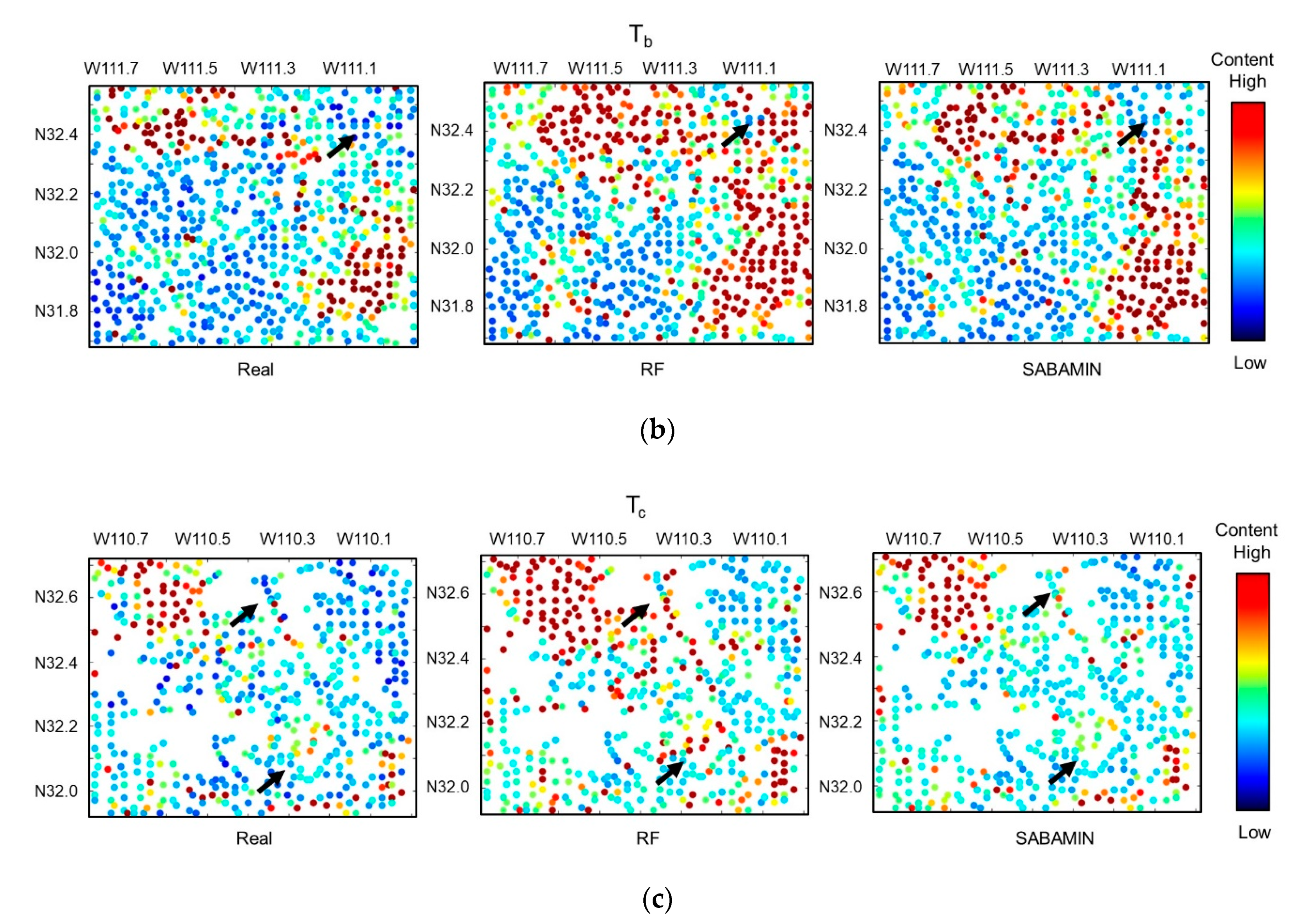
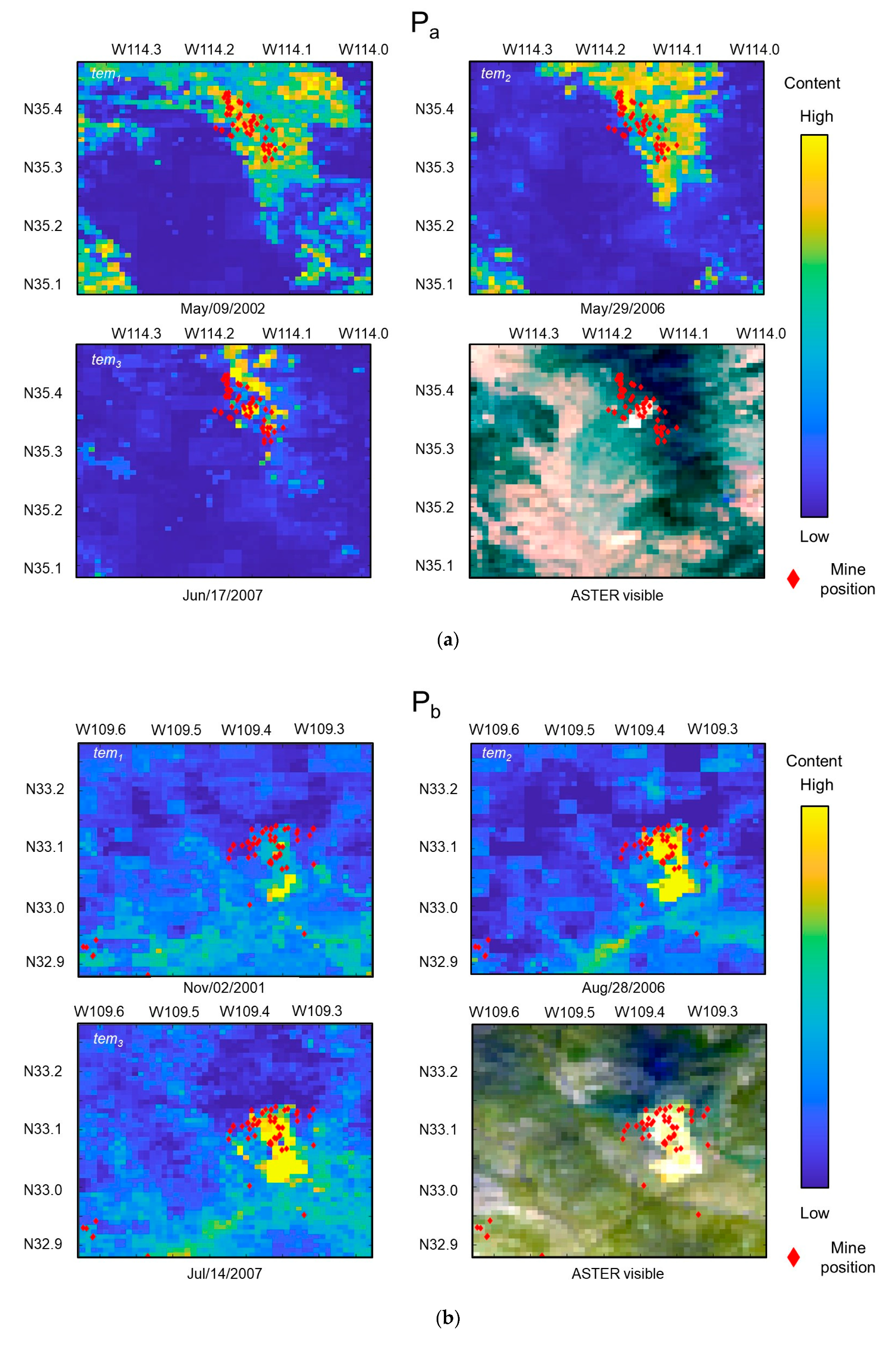
The results of the temporal stability test in the P areas by P_a, P_b, and P_c are shown in Figure 11a–c, respectively. Three predicted distributions by the remote sensing data (see Table S5 in the supplementary material) in three different temporal series (tem₁, tem₂, tem₃) approximately covering the same region are shown together in temporal order. For the reference, reconstructed images by ASTER band 1, 2, and 3N images are shown together. In all temporal series of all test areas, the copper content around a mining district was predicted to have a high value, which is considered to be a reasonable result. Even if the ASTER images were captured at different timings, the predicted distributions would look very similar.

Table 5. R_p results between pairs of tem₁, tem₂, and tem₃. Tests are repeated 30 times, with the (average ± standard deviation) listed.

Area	Rp
	tem1 vs. tem2	tem1 vs. tem3	tem2 vs. tem3
Pa	0.681 **	0.347 *	0.548 *
Pb	0.756 **	0.710 **	0.834 **
Pc	0.743 **	0.581 **	0.562 **

* p < 0.05; ** p < 0.001.

shows the similarity between the pairs of tem₁, tem₂, and tem₃, which was evaluated by R_p. All R_ps almost exceeded 0.5, which indicates that the prediction was steady temporally. The results above suggest a high reliability of our algorithm.

3.4. The Predictor Importance Test

The results of the predictor’s importance analysis by RF are shown in Figure 12 and

Table 6. Total predictor’s importance in each variable group.

Group	Predictor Number	ImG (Mean ± SD)
Geomagnetic	4	0.088 ± 0.012
DEM	2	0.088 ± 0.018
ASTER Band	28	0.210 ± 0.023
ASTER Lithological index	27	0.457 ± 0.025
Coordinates	2	0.158 ± 0.021

. From the results that show the importance of coordinates are ranked at first and third, the spatial information is the most important factor in our constructed model, which corresponds with the knowledge that spatial information is crucial for geochemical mapping, (see previous study [5,6]). Next, the altitude and slope are ranked at second and sixth, which corresponds with the fact that copper mines (high copper content areas) are always located in the mountains in the Arizona area [35], and mining changes the topographic surface. Of the four geomagnetic predictors, one was ranked in the top 10, and the remaining three were ranked in the top 20, which corresponds with the fact that metal elements influence the geomagnetics. In this copper prediction case, the ASTER lithological index obtained by cross band calculation, such as Mg-OH, muscovite, dolomite, kaolinite, silica, quartz, and alunite are in high ranks, and are commonly seen alteration minerals exposed around active mines. All the above information demonstrates that the constructed model is reasonable for geochemical contents mapping. A comprehensive look at Figure 12 and Table 6 does not show any significance that any factors were more overwhelming than all other factors. All predictors were fairly treated to construct the model.

4. Discussion

By applying the data augmentation strategy, pseudo training datasets were created using the kriging interpolation model. The accuracy of the ML model was improved with augmented data, which agree with applications in different fields [36,37]. The geochemical content in the majority positions were only at the background level, and the high regions’ performances were considered to be anomalies on the map. In a univariate interpolation, it is difficult to describe all the geological anomalies perfectly by maximum likelihood estimation using such data with high skewness; thus, usually the geological anomalies sometimes contradict the distant geospatial association. In this study, to avoid that, although we still calculated the weight by kriging, in the interpolation operation, the vacant pixels in a triangular area were only interpolated by the three most neighboring points and sacrificing the contribution by some low weight measured points. This might be the one reason that an only slight improvement of RMSE was observed in our study. Recently, Kim et al. [38] proposed a curvature interpolation method which is suggested to be a more accurate univariate interpolation method for geospatial data than IDW, and is considered a candidate method to improve the accuracy of pseudo training data generation. ML usually only constructs a model to fit the majority in the datasets, where the minority tends to be ignored by the model. As a result, the high values are underestimated. This might be another reason for slight RMSE improvement. By the hint of mineral prospectivity mapping studies [39,40,41], the geochemical distribution can be treated as classification labels. It is observed from Figure 10 that, although predicted distribution does not perfectly correspond with the real one, a high accuracy of classifying high and low contents should be achieved. Therefore, the prediction accuracy can be further improved using the method that firstly classifies the study area into different classes, and then constructs different regression models in the different region with different class to ensure all data can be correctly estimated in specific ranges.

In the temporal stability test, ASTER images in different temporal series were used for the test. We hypothesized that there was no or only slightly topography alteration in the short term, and by ignoring some human-made changes, ASTER images in different temporal series should be the same. Therefore, the predicted geochemical distribution should be similar in this case. However, the ASTER images show the solar optical reflectance information from the Earth’s surface, and despite the effect of the surface vegetation coverage condition, the reflected luminance may change due to different solar heights and angles at different times in the day or during different seasons. This unstable component was regarded as signal noise in temporal series. Although it is possible to achieve a higher similarity in P_a, P_b, and P_c by correcting them in accordance with the solar zenith angle [42], a reasonable result that predicted high content regions are located at or very near to actual mining districts in all temporal series indicated that our prediction model was robust to this fluctuation induced by solar condition changing. Thus, the signal of the predictor variables seem to be more determinative than the noise in the prediction process.

5. Conclusions

In this study, to provide a high accuracy model for generating a high-resolution geochemical map, we proposed a new algorithm, SABAMIN, which merged both spatial location and autocorrelation into an ML model by using data augmentation and computational geometry strategies. We applied kriging interpolation to generate pseudo training datasets and applied an alpha shape method to build these pseudo training datasets to become geologically reliable.

In the blind test results, a higher similarity meant the spatial autocorrelation was reserved well in the prediction model. Furthermore, coordinate variables were ranked at the top level in the predictor’s importance test. These results suggest that we successfully merged spatial autocorrelation into the ML model by only co-training with the sampled datasets and pseudo training datasets.

Compared with the RF constructed model, SABAMIN achieved a lower RMSE in the cross-validation test. The model also performed a steady prediction in a temporal stability test using multiple ASTER images in different temporal series. The effect and reliability were confirmed by these results.

According to the ranking of predictor importance, the machine learning suggested that the major factor related to copper content distribution corresponded with common geological knowledge, which suggests that the constructed model is reasonable for geochemical contents mapping.

In summary, SABAMIN is effective for generating high-resolution geochemical maps with high accuracy. Combining the univariate interpolation method with multivariate prediction with data augmentation also proved effective for geological studies.

In the future, we will further improve the pseudo training data generation method or try to provide different prediction model to different region with contents in different levels to improve the accuracy of the prediction model.

References

- Pal, M.; Rasmussen, T.; Porwal, A. optimized lithological mapping from multispectral and hyperspectral remote sensing images using fused multi-classifiers. Remote Sens. 2020, 12, 177. [Google Scholar] [CrossRef] [Green Version]
- Kirkwood, C.; Cave, M.; Beamish, D.; Grebby, S.; Ferreira, A. A machine learning approach to geochemical mapping. J. Geochem. Explor. 2016, 167, 49–61. [Google Scholar] [CrossRef] [Green Version]
- Gahegan, M. On the application of inductive machine learning tools to geographical analysis. Geogr. Anal. 2000, 32, 113–139. [Google Scholar] [CrossRef]
- Mather, P.M.; Koch, M. Computer Processing of Remotely-Sensed Images: An introduction; John Wiley & Sons: Hoboken, NJ, USA, 2011; pp. 1–75. [Google Scholar]
- Cracknell, M.J.; Reading, A.M. Geological mapping using remote sensing data: A comparison of five machine learning algorithms, their response to variations in the spatial distribution of training data and the use of explicit spatial information. Comput. Geosci. 2014, 63, 22–33. [Google Scholar] [CrossRef] [Green Version]
- Sergeev, A.P.; Buevich, A.G.; Baglaeva, E.M.; Shichkin, A.V. Combining spatial autocorrelation with machine learning increases prediction accuracy of soil heavy metals. Catena 2019, 174, 425–435. [Google Scholar] [CrossRef]
- Tanner, M.A.; Wong, W.H. The calculation of posterior distributions by data augmentation. J. Am. Stat. Assoc. 1987, 82, 528–540. [Google Scholar] [CrossRef]
- Liu, J.S.; Wu, Y.N. Parameter expansion for data augmentation. J. Am. Stat. Assoc. 1999, 94, 1264–1274. [Google Scholar] [CrossRef]
- Perez, L.; Wang, J. The effectiveness of data augmentation in image classification using deep learning. arXiv 2017, arXiv:1712.04621. Available online: https://arxiv.org/abs/1712.04621v1 (accessed on 7 December 2016).
- Kleijnen, J.P. Kriging metamodeling in simulation: A review. Eur. J. Oper. Res. 2009, 192, 707–716. [Google Scholar] [CrossRef] [Green Version]
- Breiman, L. Random forests. Mach. Learn. 2001, 45, 5–32. [Google Scholar] [CrossRef] [Green Version]
- Huang, C.; Shibuya, A. Approach for generating high accuracy machine learning model for high resolution geochemical map completion using remote sensing data: Case study of Arizona, USA. In Earth Resources and Environmental Remote Sensing/GIS Applications X; SPIE: Strasbourg, France, 2019; p. 111560F. [Google Scholar] [CrossRef]
- Shepard, D. A two-dimensional interpolation function for irregularly-spaced data. In Proceedings of the 1968 23rd ACM National Conference, New York, NY, USA, 27–29 August 1968; ACM: New York, NY, USA, 1968; pp. 517–524. [Google Scholar]
- McBratney, A.B.; Webster, R. Choosing functions for semi-variograms of soil properties and fitting them to sampling estimates. J. Soil Sci. 1986, 37, 617–639. [Google Scholar] [CrossRef]
- Cressie, N. Statistics for Spatial Data; Revised Edition; John Wiley & Sons: Hoboken, NJ, USA, 1993; pp. 1–275. [Google Scholar]
- Lang, J.R.; Titley, S.R. Isotopic and geochemical characteristics of laramide magmatic systems in Arizona and implications for the genesis of porphyry copper deposits. Econ. Geol. 1998, 93, 138–170. [Google Scholar] [CrossRef]
- Bodnar, R.J.; Beane, R.E. Temporal and spatial variations in hydrothermal fluid characteristics during vein filling in preore cover overlying deeply buried porphyry copper-type mineralization at Red Mountain, Arizona. Econ. Geol. 1980, 75, 876–893. [Google Scholar] [CrossRef]
- Manske, S.L.; Paul, A.H. Geology of a major new porphyry copper center in the Superior (Pioneer) district, Arizona. Econ. Geol. 2002, 97, 197–220. [Google Scholar] [CrossRef]
- Abrams, M.J.; Brown, D.; Lepley, L.; Sadowski, R. Remote sensing for porphyry copper deposits in southern Arizona. Econ. Geol. 1983, 78, 591–604. [Google Scholar] [CrossRef]
- Smith, S.M. National Geochemical Database Reformatted Data from the National Uranium Resource Evaluation (NURE) Hydrogeochemical and Stream Sediment Reconnaissance (HSSR) Program; US Geological Survey, US Dept. of the Interior: Washington, DC, USA, 1997; pp. 97–492. Available online: https://pubs.usgs.gov/of/1997/ofr-97-0492/ (accessed on 7 December 2016).
- Smith, S.M. A Manual for Interpreting USGS-Reformatted NURE HSSR Data Files; USGS Publications Warehouse: Reston, VA, USA, March 2006. Available online: https://pubs.usgs.gov/of/1997/ofr-97-0492/nure_man.htm (accessed on 7 December 2016).
- Schruben, P.G.; Arndt, R.E.; Bawiec, W.J. Geology of the Conterminous United States at 1: 2,500,000 Scale a Digital Representation of the 1974 PB King and HM Beikman Map; Technical Report No. 11; The Survey; For sale by USGS Map Distribution; USGS: Reston, VA, USA, 1998. Available online: https://pubs.usgs.gov/dds/dds11/ (accessed on 7 December 2016).
- Mason, G.T.; Arndt, R.E. Mineral Resources Data System (MRDS); No. 20; USGS Numbered Series; USGS: Reston, VA, USA, 1996. [CrossRef]
- McFaul, E.J.; Mason, G.T.; Ferguson, W.B.; Lipin, B.R. U.S. Geological Survey Mineral Databases; Technical Report No. 50; MRDS and MAS/MILS: Reston, VA, USA, 2000. [CrossRef]
- Bankey, V.; Cuevas, A.; Daniels, D.; Finn, C.A.; Israel, H.; Hill, P.; Kucks, R.; Miles, W.; Pilkington, M.; Roberts, C.; et al. Digital Data Grids for the Magnetic Anomaly Map of North America; USGS Open-File Report 02-414; USGS: Reston, VA, USA, 2002. Available online: https://pubs.usgs.gov/of/2002/ofr-02-414 (accessed on 25 October 2002).
- Van der Meer, F.D.; Van der Werff, H.M.; Van Ruitenbeek, F.J.; Hecker, C.A.; Bakker, W.H.; Noomen, M.F.; Van der Meijde, M.; Carranza, E.J.M.; Van de Smeth, J.B.; Woldai, T. Multi-and hyperspectral geologic remote sensing: A review. Int. J. Appl. Earth Obs. 2012, 14, 112–128. [Google Scholar] [CrossRef]
- Ninomiya, Y.; Fu, B. Spectral indices for lithologic mapping with ASTER thermal infrared data applying to a Part of Beishan Mountains. In Proceedings of the IEEE 2001 International Geoscience and Remote Sensing Symposium (Cat. No. 01CH37217), IEEE, Sidney, Australia, 9–13 July 2001; pp. 2988–2990. [Google Scholar]
- Lindsay, M.D.; Betts, P.G.; Ailleres, L. Data fusion and porphyry copper prospectivity models, southeastern Arizona. Ore Geol. Rev. 2014, 61, 120–140. [Google Scholar] [CrossRef]
- Yigit, O. A prospective sector in the tethyan metallogenic belt: Geology and geochronology of mineral deposits in the biga peninsula, NW Turkey. Ore Geol. Rev. 2012, 46, 118–148. [Google Scholar] [CrossRef]
- Abedi, M.; Norouzi, G.H. Integration of various geophysical data with geological and geochemical data to determine additional drilling for copper exploration. J. Appl. Geophys. 2012, 83, 35–45. [Google Scholar] [CrossRef]
- Edelsbrunner, H.; Kirkpatrick, D.; Seidel, R. On the shape of a set of points in the plane. IEEE Trans. Inf. Theory 1983, 29, 551–559. [Google Scholar] [CrossRef] [Green Version]
- Guibas, L.; Stolfi, J. Primitives for the manipulation of general subdivisions and the computation of Voronoi. ACM Trans. Graph. 1985, 4, 74–123. [Google Scholar] [CrossRef]
- Sutherland, I.E.; Sproull, R.F.; Schumacker, R.A. A characterization of ten hidden-surface algorithms. ACM Comput. Surv. 1974, 6, 1–55. [Google Scholar] [CrossRef]
- Nilufar, S.; Morrow, A.A.; Lee, J.M.; Perkins, T.J. FiloDetect: Automatic detection of filopodia from fluorescence microscopy images. BMC Syst. Biol. 2013, 7, 66. [Google Scholar] [CrossRef] [PubMed] [Green Version]
- Ayuso, R.A.; Barton, M.D.; Blakely, R.J.; Bodnar, R.J.; Dilles, J.H.; Gray, F.; Graybeal, F.T.; Mars, J.C.; McPhee, D.K.; Seal, R.R.; et al. Porphyry Copper Deposit Model: Chapter B in Mineral Deposit Models for Resource Assessment; Technical Report No. 2010-5070-B; US Geological Survey: Reston, VA, USA, 2010; pp. 1–130. Available online: https://pubs.usgs.gov/sir/2010/5070/b/ (accessed on 7 December 2016).
- Tran, T.; Pham, T.; Carneiro, G.; Palmer, L.; Reid, I. A bayesian data augmentation approach for learning deep models. In Advances in Neural Information Processing Systems; NIPS: Long Beach, CA, USA, December 2017; pp. 2797–2806. [Google Scholar]
- Salamon, J.; Bello, J.P. Deep convolutional neural networks and data augmentation for environmental sound classification. IEEE Signal Process. Lett. 2017, 24, 279–283. [Google Scholar] [CrossRef]
- Kim, H.; Willers, J.L.; Kim, S. The curvature interpolation method for surface reconstruction for geospatial point cloud data. Int. J. Remote Sens. Appl. 2020, 41, 1512–1541. [Google Scholar] [CrossRef]
- Chen, Y.; Wu, W. Mapping mineral prospectivity using an extreme learning machine regression. Ore Geol. Rev. 2017, 80, 200–213. [Google Scholar] [CrossRef]
- Carranza, E.J.M.; Laborte, A.G. Random forest predictive modeling of mineral prospectivity with small number of prospects and data with missing values in Abra (Philippines). Comput. Geosci. 2015, 74, 60–70. [Google Scholar] [CrossRef]
- Abedi, M.; Norouzi, G.H.; Bahroudi, A. Support vector machine for multi-classification of mineral prospectivity areas. Comput. Geosci. 2012, 46, 272–283. [Google Scholar] [CrossRef]
- Lloyd, C.D. Local Models for Spatial Analysis; CRC Press: Boca Raton, FL, USA, 2011; p. 336. [Google Scholar]
Figure 1.
The region of interest (ROI) and the position study area in this research: (a) The approximate position in the USA; (b) the detailed study area, the boundaries of Arizona, the reference geological map of the study area, and spatially-scattered geochemical data points in this area. Different geological/lithological (G/L) types are numbered and marked in different colors. Each correspondent lithological type is referenced in Table S1 of supplementary. Sampled copper points concentrated in different positions on the map are marked as PG1, PG2, and PG3. The study areas are marked as Ta, Tb, Tc, Pa, Pb, and Pc. (c) The statistics of sampled copper data amounts and average content of all sampled copper data in each lithological type area.
Figure 2.
Study area details of: (a) Ta; (b) Tb; (c) Tc. The sampled copper data are plotted by black circles on the reference geological map, and the circle radius is proportional to the copper content. The G/L types in this figure are marked the same number of those in Figure 1.
Figure 3.
Study areas of: (a) Pa; (b) Pb; (c) Pc. The sampled copper data are plotted by black circles, and the copper mine positions referenced in the United States Geological Survey (USGS) are plotted by red diamonds. The G/L types in this figure are marked the same number of those in Figure 1.
Figure 4.
Flow chart of spatial autocorrelation-based mixture interpolation (SABAMIN) algorithm.
Figure 5.
Conceptual drawings of Figure 1 to explain how to spatially divide kriging interpolation regions and machine learning (ML) regions on a geochemical map: (a) The case of only setting a single r by fusing all sampled points in the study area to kriging interpolation. Distribution crosstalk Cr1 occurs in the regions near the border of different geological areas; (b) Delaunay triangles (DTs) generated by applying the alpha shape algorithm without setting Φ. Crosstalk Cr2 occurs at the intermediate parts between different PGs; (c) DTs generated by applying the alpha shape algorithm with setting threshold at Φt. Remaining crosstalk Cr3 occurs at the intermediate parts between different PG_Geoψ,ωs; (d) a geological mask M_Geoψ is applied; Cr3 is also eliminated.
Figure 6.
Applying the alpha shape algorithm to our case: (a) Specifying Φt by triangle thresholding algorithm; (b) alpha shape under the condition of setting Φ to infinity; (c) alpha shape under the condition of setting Φ to Φ1 < Φ < +∞; (d) alpha shape under the condition of setting Φ to Φ1.
Figure 7.
Completed kriging interpolation copper content distribution map. Colored parts are defined as T areas and white parts are defined as P areas.
Figure 8.
Flow chart of pseudo training dataset generation processing in our case.
Figure 9.
Ten-fold cross-validation results of random forests (RFs) (dots) and SABAMIN (triangles). The asterisk means there is a significant difference (p < 0.05) between them.
Figure 10.
Blind test results of (a) Ta, (b) Tb, and (c) Tc.
Figure 11.
Temporal stability tests in P area results of (a) Pa, (b) Pb, and (c) Pc. Red diamonds show the mine position. The crowd of the mine positions corresponds with the mining district shown in Figure 3.
Figure 12.
Importance of all predictors.