Article

Fusion of Five Satellite-Derived Products Using Extremely Randomized Trees to Estimate Terrestrial Latent Heat Flux over Europe

1
State Key Laboratory of Remote Sensing Science, Faculty of Geographical Science, Beijing Normal University, Beijing 100875, China
2
Jincheng Meteorological Administration, Jincheng 048026, China
*
Author to whom correspondence should be addressed.
Submission received: 24 December 2019 / Revised: 14 February 2020 / Accepted: 18 February 2020 / Published: 19 February 2020
(This article belongs to the Special Issue Hydrometeorological Prediction and Mapping)

Abstract

:
An accurate estimation of spatially and temporally continuous latent heat flux (LE) is essential in the assessment of surface water and energy balance. Various satellite-derived LE products have been generated to enhance the simulation of terrestrial LE, yet each individual LE product shows large discrepancies and uncertainties. Our study used Extremely Randomized Trees (ETR) to fuse five satellite-derived terrestrial LE products to reduce uncertainties from the individual products and improve terrestrial LE estimations over Europe. The validation results demonstrated that the estimation using the ETR fusion method increased the R2 of five individual LE products (ranging from 0.53 to 0.61) to 0.97 and decreased the RMSE (ranging from 26.37 to 33.17 W/m2) to 5.85 W/m2. Compared with three other machine learning fusion models, Gradient Boosting Regression Tree (GBRT), Random Forest (RF), and Gaussian Process Regression (GPR), ETR exhibited the best performance in terms of both training and validation accuracy. We also applied the ETR fusion method to implement the mapping of average annual terrestrial LE over Europe at a resolution of 0.05 ◦ in the period from 2002 to 2005. When compared with global LE products such as the Global Land Surface Satellite (GLASS) and the Moderate Resolution Imaging Spectroradiometer (MODIS), the fusion LE using ETR exhibited a relatively small gap, which confirmed that it is reasonable and reliable for the estimation of the terrestrial LE over Europe.

Graphical Abstract

1. Introduction

The latent heat flux (LE) governs the associated heat flux of the interaction between land surface and its atmosphere [1], including vegetation transpiration, soil evaporation, and plant canopies interception evaporation [2]. In general, LE returns approximately 60% of rain back to the atmosphere and also helps to cool the land surface by consuming an enormous amount of heat [3]. Europe makes up the western fifth of the Eurasian landmass. Thus, an accurate LE estimation over Europe plays a key role in many climatic, hydrologic, and agricultural applications [4]. As a confederation of regional observation networks, FLUXNET routinely provides long-term eddy covariance (EC) flux measurements of carbon, water vapor, and energy exchange over America, Europe, Asia, Africa, and Australia. About one-third of FLUXNET’s EC sites are located in Europe. However, as result of the spatial heterogeneity, point-based measurements of terrestrial LE cannot be applied for continuous monitoring on a large scale [5].
Satellite-based observations can provide us with a more readily available monitoring for land surface and atmospheric properties. Combined with well-known flux equations [6,7], we can effectively derive spatially and temporally continuous LE estimates over large areas. Currently, various satellite-derived LE products at moderate spatial resolution are generated, including the Moderate Resolution Imaging Spectroradiometer (MODIS) LE product (MOD16) with a resolution of 0.5 km / 1 km and 8 days [8,9], the Global Land Evaporation Amsterdam Model (GLEAM) LE product with a resolution of 0.25 ◦ and 1 day [10], the Global Land Surface Satellite (GLASS) LE product with a resolution of 1 km / 5 km and 8 days [11], or the Breathing Earth System Simulator (BESS) LE product with a resolution of 1 km and 8 days [12]. However, when intercomparing and evaluating with long-term ground measurements from in situ flux networks, satellite-derived LE products showed large discrepancies. Previous studies over China [13,14], Brazil [15], Spain [16], and South Africa [17] found that in the arid and semiarid climate, MOD16 underestimated the LE of the irrigated crop in the growing season [18]. Additionally, some reanalysis and data assimilation LE products have a relatively high temporal resolution but a relatively coarse spatial resolution, such as the Global Land Data Assimilation System (GLDAS) datasets with 0.25 degree spatial resolution and 3 hour temporal resolution [19,20]. Validation against tower flux measurements indicates that LE datasets with a relatively coarse spatial resolution tend to contain large uncertainties regarding the heterogeneous terrestrial biosphere [2]. Therefore, deriving terrestrial LE estimates accurately with both a high spatial resolution (e.g., 1 km) and a reasonable temporal resolution (e.g., daily) remains a central challenge.
To meet this demand, many satellite-derived algorithms are designed to implement LE terrestrial estimates, mainly using process-based algorithms and empirical/semi-empirical algorithms, etc. Traditional process-based algorithms, such as the Surface Energy Balance System (SEBS) [21], the Single-Source models [21,22,23,24], the Two-Source models [25,26,27,28,29,30], the Penman–Monteith (PM) equation [8,9], and the Priestley–Taylor (PT) algorithm [7,31,32,33], calculate terrestrial LE using satellite-derived datasets related to meteorological observations based on the surface energy balance (SEB) equation [34]. However, as a result of the uncertainties that exist in different model structures, the simulation results of each algorithm show large discrepancies [35]. Empirical/semi-empirical algorithms are convenient to apply but the need to determine the site-specific parameters makes them difficult to implement accurately with variable surface conditions [36]. As the most viable empirical algorithms, machine learning methods have demonstrated great success in predicting complex problems and have been widely used to estimate LE. For instance, Wang [37] used artificial neural network (ANN) combined with meteorological parameters, remote sensing variable (NDVI), and ground-measured LE from 85 EC flux tower sites to predict LE over North America. Bodesheim et al. [38] obtained a global half-hourly LE product using FLUXNET observations, remotely sensed and meteorological data with the Random Forests (RF) method. Xu et al. [39] generated daily ET from in situ flux tower sites on the Heihe River Basin scale at a spatial resolution of 1km by using remote sensing variables (LAI, land cover), air temperature (Ta), relative humidity (RH), solar radiation (Rs), and precipitation (P) with the RF method. However, simulation under complex heterogeneity conditions by these data-driven methods remains questionable because of the spatial representation limitation of sparse training data at certain sites.
Far from discouraging the development of LE simulation methods over large scales, the discrepancies and uncertainties lie in the individual LE products, thus providing an opportunity to foster further research. In recognition of above challenges, the approach of fusing multiple LE products would be preferable. Aiming to develop effective fusion methods, these efforts have ranged from the simple model averaging method (SMA) [40] to more complex approaches such as Bayesian model averaging (BMA) [11], empirical orthogonal function (EOF) [41], or integration methodologies considering consistency with water cycle products [42]. Yao et al. generated the GLASS LE product by fusing of five LE products using the BMA method to enhance terrestrial daily LE estimates [11]. Zhu et al. also reported that merging ET products using the BMA method can achieve more reliable estimations than the SMA method across north China [43]. However, a limitation associated with these fusion methods concerning the weight calculating efficiency of the individual products has somewhat affected their wider application [2]. Regarding this, approaches involving multiple LE product ensembles based on machine learning techniques have the potential to provide accurate terrestrial LE estimates. Extremely Randomized Trees (ETR) as a new tree-based machine learning ensemble method has shown better robustness and regression accuracy compared with other traditional models [44]. Experiments show that ETR is generally competitive and even superior to RF in terms of accuracy [45]. Although ETR has been substantially applied to regression approaches, there is a lack of experiments on datasets fusion problems, especially in improving terrestrial LE estimates by merging multiple LE products
With the aim of reducing uncertainties in individual satellite-derived LE products, in this study, we used Extremely Randomized Trees (ETR) to enhance terrestrial LE estimations over Europe by fusing five individual LE products. We had three major objectives: (1) to evaluate individual satellite-derived terrestrial LE products produced by five classic LE algorithms using ground-measured EC data from the FLUXNET; (2) to evaluate the ETR fusion method by comparing it with three other machine learning methods using the EC observations and two other global LE products; and (3) to apply the ETR method to map the mean annual terrestrial LE with 0.05° spatial resolution in the period from 2002 to 2005 based on MODIS and Modern Era Retrospective Analysis for Research and Applications (MERRA) meteorological data over Europe.

2. Data

We produced individual satellite-derived terrestrial LE products using five traditional LE algorithms. Table 1 describes the five LE products in detail. The forcing data included MODIS Fraction of Absorbed Photosynthetically Active Radiation (FPAR) data with 500m spatial resolution, MODIS NDVI and GLASS LAI data with a 0.05 degrees spatial resolution, MERRA meteorological data with a 1/2 * 2/3 degrees spatial resolution. The daily surface net radiation (Rn), shortwave radiation (Rs), relative humidity (RH), air temperature (Ta), vapor pressure (e), and wind speed (WS) from MERRA were used in this study. The FPAR and MERRA meteorological data were spatially interpolated into 0.05 degrees by the bilinear method in order to be consistent with the MODIS pixel size. The individual LE products are briefly described in the following.

2.1. Satellite-Derived Terrestrial LE Products

2.1.1. Revised Remote Sensing-Based Penman (RS-PM)- LE Product

The RS-PM-based LE product was generated by an improved Penman–Monteith equation [9]. The total LE consisted of four components: the canopy transpiration (LEc), interception evaporation (LEi), saturated wet soil evaporation (LEws), and unsaturated soil evaporation (LEds). FPAR was used as an improved vegetation cover fraction. The calculations of aerodynamic, boundary-layer, and canopy resistance were also modified compared to the beta version [11]. A more detailed description of the RS-PM algorithm can be found from Mu et al. (2011) [9]. The input variables include Rn, Ta, Tmin, RH, and e from the MERRA data, FPAR derived from the MOD15C2 product, and LAI derived from the GLASS product. The daily RS-PM-based LE product has a 0.05 degrees resolution and covers Europe from 2000 to 2006.

2.1.2. Shuttleworth–Wallace Dual-Source (SW)-Based LE Product

The SW-based LE product was generated by the Shuttleworth–Wallace dual-source (SW) model [46]. On the basis of the energy balance theory, the SW algorithm divided the total LE into two components: the vegetation transpiration (LEv) and the soil evaporation (LEs). Assuming aerodynamic mixing occurring at a mean canopy source height within the canopy [35], the LEv and LEs can be estimated separately using two Penman–Monteith equations. A more detailed description of the SW algorithm can be obtained from Shuttleworth and Wallace (1985) [46]. The input variables include WS, Rn, Ta, RH, and e from the MERRA data and GLASS LAI. The daily SW LE product covers Europe with a 0.05 degrees spatial resolution for the period from 2000 to 2006.

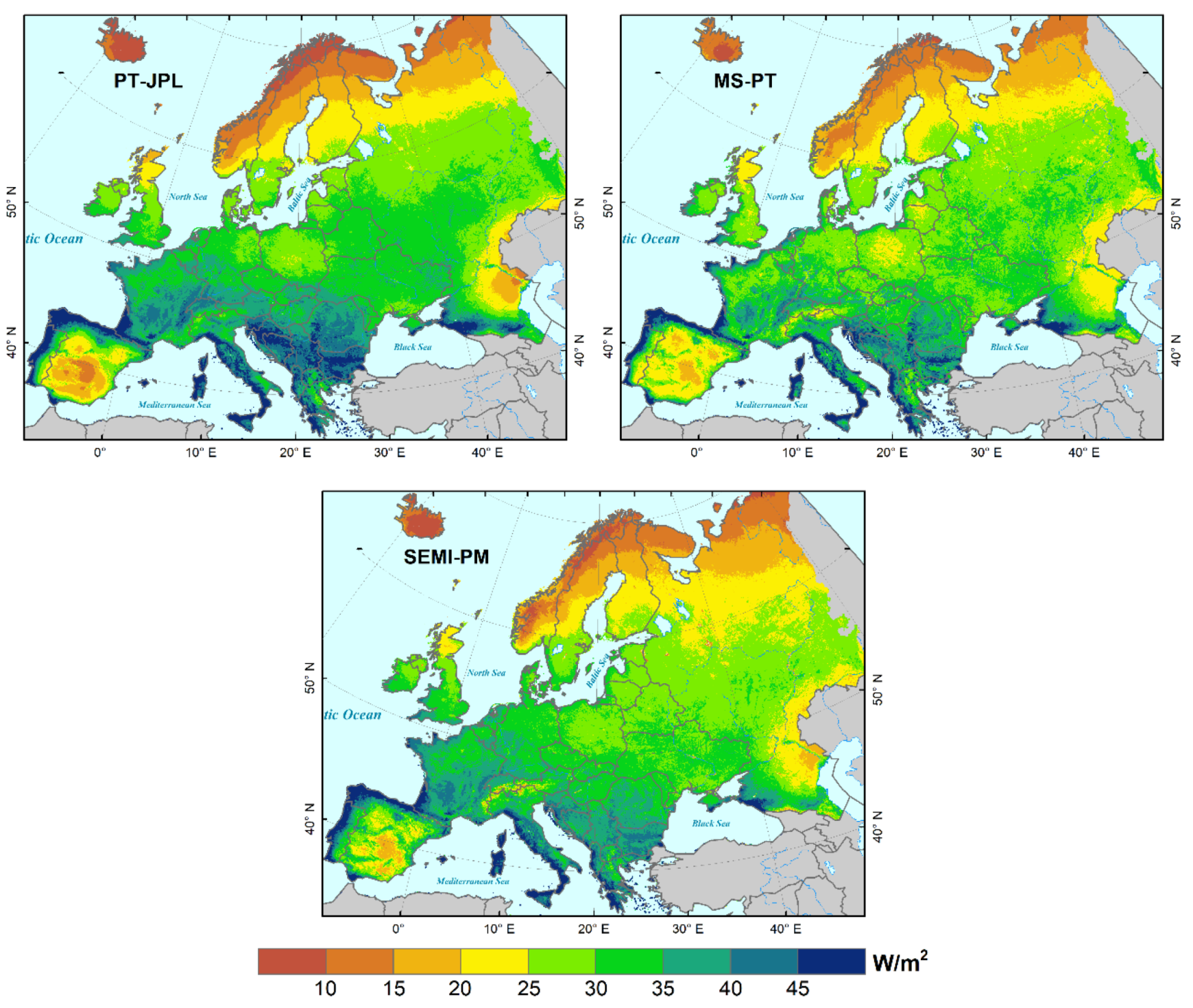
2.1.3. Priestley-Taylor of the Jet Propulsion Laboratory (PT-JPL)-Based LE Product

The PT-JPL-based LE product was generated by a novel Priestley–Taylor equation proposed by Fisher et al. [31]. The atmospheric constraints (RH, Vapor Pressure Deficit) and ecological constraints (LAI, FPAR) were associated to determine dynamic coefficients to transform potential ET to actual ET [7]. The extended empirical parameters were determined without using any ground measurements. More formal information about the PT-JPL can be obtained from Fisher et al. (2008) [31]. The input variables to generate the PT-JPL-based LE product include Rn, RH, Ta, and e from the MERRA data, NDVI and FPAR derived from the MODIS product, and LAI derived from the GLASS product. The daily PT-JPL-based LE product covers Europe during the period from 2000 to 2006 with a spatial resolution of 0.05 degrees.

2.1.4. Modified Satellite-Based Priestley–Taylor (MS-PT)-Based LE Product

The MS-PT-based LE product was generated by a modified satellite-based PT (MS-PT) model proposed by Yao et al. [32]. The MS-PT algorithm separated LE into four components: the canopy transpiration (LEc), vegetation interception evaporation (LEi), unsaturated soil evaporation (LEds), and saturated wet soil evaporation (LEws). The diurnal air temperature range (DT) was used to quantify the apparent thermal inertia (ATI), which parameterized surface soil moisture (SM) constraints [2]. It only requires four parameters as input: the surface net radiation, air temperature, DT, and NDVI. A more formal introduction to the MS-PT algorithm can be obtained from Yao et al. (2013) [32]. The LE product input variables include Rn, Ta, Tmax, and Tmin from the MERRA data and MODIS NDVI data. The MS-PT LE product has the same spatial and temporal resolution as the PT-JPL-based LE product from 2000 to 2006.

2.1.5. Semi-Empirical Penman Algorithm (SEMI-PM)-Based LE Product

The SEMI-PM-based LE product was generated by a Semi-empirical Penman algorithm (SEMI-PM) equation proposed by Wang et al. [47]. The obvious difference between this algorithm and the other four is that the SEMI-PM used wind speed to make the terrestrial LE estimation, which may influence the annual or decadal LE variability [11]. The empirical coefficients for this algorithm were calibrated by 64 global flux tower sites, and the average correlation coefficient of this algorithm was up to 0.94. More formal information about SEMI-PM can be acquired from Wang et al. (2010) [47]. The SEMI-PM LE product requires Rs, Ta, WS, and RH from the MERRA data and MODIS NDVI data. This daily LE product with a 0.05 degrees spatial resolution is also available over Europe during the period from 2000 to 2006.

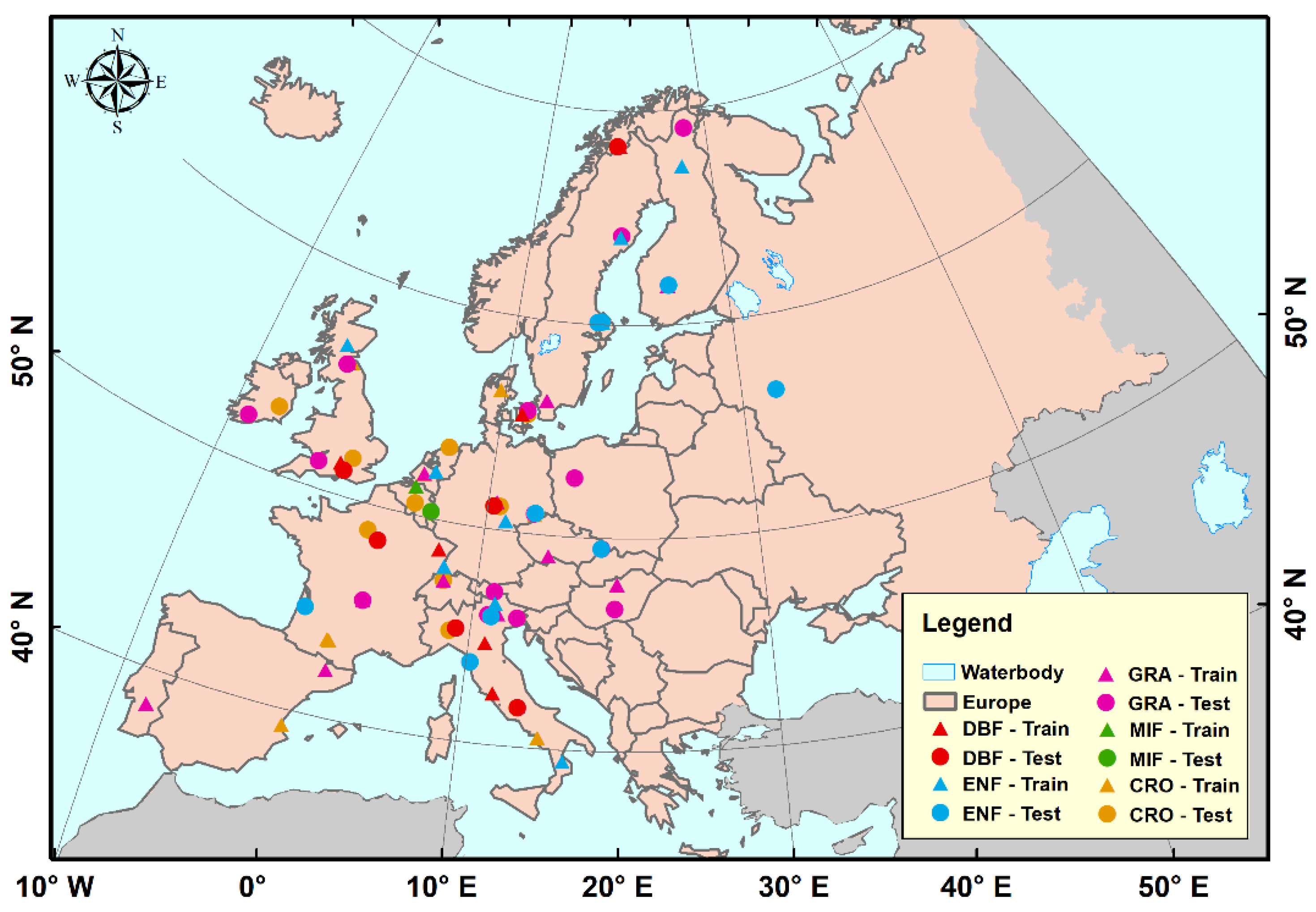
2.2. Eddy Covariance Data

Our study used FLUXNET eddy covariance (EC) data to evaluate and validate the five satellite-derived terrestrial LE products and four machine learning fusion methods. The ground measurements were mainly gathered from 76 Europe flux tower sites (Figure 1) and each site spanned more than one growing season from 2000 to 2009. These sites were covering five major plant function types (PFTs): deciduous broadleaf forest (DBF, 12 sites), evergreen needleleaf forest (ENF, 18 sites), grassland (GRA, 27 sites), mixed forest (MIF, 2 sites), cropland (CRO, 17 sites), and these PTFs represent the major terrestrial biomes in Europe. Evenly distributed in space, half of the sites were uniformly chosen to train the machine learning models, and the rest of the sites were used to validate the model fusion performance. These ground-measured data included half-hourly or hourly Rn, ground heat flux (G), Rs, WS, Ta, RH, e, sensible heat flux (H), and LE. Because the EC observation method suffers a problem related with energy imbalance, the sum of obtained H and LE is generally less than the total available energy [48]. Therefore, the measured LE can be corrected as follows [49]:
L E c o r = ( R n G ) / ( H u n c o r +   L E u n c o r ) ×   L E u n c o r
where L E c o r is the corrected LE, and the H u n c o r and L E u n c o r are the uncorrected H and LE, respectively.

3. Methods

3.1. Extremely Randomized Trees

Extremely Randomized Trees (Extra-Trees, ET) proposed by Geurts is a tree-based machine learning ensemble model for supervised learning of classification and regression [50]. Extra-Trees Regression (ETR) constructs an ensemble of regression trees based on a classical top-down procedure. The obvious discrepancy with other ensemble models is that ETR constructs the trees with all the learning sample instead of a bootstrap replica, and it selects a random cut-point for each feature under consideration rather than computing a locally optimal one [50]. ETR has three important parameters: the K, nmin, and M. These three parameters can be adapted to the specific case either manually or automatically, using cross-validation for example.
The parameter K denotes the number of random splits and its available range is 1 to n, where n denotes the number of attributes. The smaller the K is, the stronger the randomization of the trees will be. Experiments have shown that the optimal values of K are K = n for classification and K = n for regression [50].
The parameter nmin denotes the sample counts to split a node. Lager nmin leads to a higher bias and smaller of both trees and variances. Optimal default values of nmin depend, in principle, on the output dataset noise. Fully grown trees will generate a very noisy output which always leads to an over-fit problem.
The parameter M is the count of trees. The more trees, the better accuracy, in principle [51]. The compromise between computational requirements and accuracy is the deciding factor for the choice of an appropriate value of M.
The score measure in ETR is the relative variance reduction. For a sample S and a split s , the score is defined as follows:
S c o r e ( s , S ) =   v a r { y | S }   | S l | | S | v a r { y | S l }   | S r | | S | v a r { y | S r } v a r { y | S }
where S l and S r denote the two subsets of cases from S corresponding to the two outcomes of a split s . The v a r { y | S } represents the variance of the output y in the sample S .
The ETR method has no need for the optimization of the discretization thresholds, so it is competitive with other ensemble models in terms of the accuracy, computing times, and ease of implementation.

3.2. Other Machine Learning Fusion Methods

3.2.1. Gradient Boosting Regression Tree

The Gradient Boosted Regression Tree (GBRT) model, also known as the gradient boosting decision tree, is a boosting regression model consisting of an ensemble of decision trees [52]. GBRT builds the model by a stage-wise way, and it generalizes them by optimizing an arbitrary loss function. The approximation function for GBRT can be expressed as
f ( x ) = n = 1 N β m h ( x ; a n )
where β m denotes the weight for an individual decision tree h ( x ; a n ) . Each individual decision tree can be defined as follows:
h ( x ; a n ) =   m = 1 M γ m n I   ( x R m n )
where x represents the input variables, and a n denotes the classifier of each decision tree. The input dataset would be parted into M regions by the trees. The γ m n represents the predicted constant for the corresponding region.
The GBRT can generate an appropriate nonlinear relationship automatically by the ensemble trees [53] and process skewed variables without transformations. GBRT can overcome the problem of over-fitting by combining hundreds of weak decision trees. The computational robustness and high scalability of GBRT make it a superior model as compared to a single decision tree [54].

3.2.2. Random Forests

Random Forests (RF) [51] as an enhancement of bagging [55] is an ensemble of single trees. The independent tree predictor in the ensemble is generated by randomly selecting input variables using the bootstrap [56] sampling method. The optimal split can be found either from all input variables or a preset-sized random subset during the construction of a single tree. The estimate variance of the trees can be reduced by increasing the randomness. Experiments found that RF methods significantly outperform other decision tree methods because the single trees typically generate high variance and are prone to over-fit [50]. The randomness injected into forests when generating decision trees may decouple prediction errors. Some errors can be cancelled out by taking an average of those predictions. As a result of the low correlation between independent trees, the RF can avoid falling into over-fitting problems in the process of regression [39].

3.2.3. Gaussian Process Regression

The Gaussian Process Regression (GPR) algorithm is a classical stochastic process method in probability theory. The GPR is a combination of random variables obeying the normal distribution [57]. The kernel of GPR is the Gaussian Process (GP) learning framework which is competitive in handling nonlinear relationships [58]. The kernel function of GPR is GP, which is a collection of finite random variables with a Gaussian distribution that can be used to describe the distribution of functions. The output data y and the input vector x can be expressed as
y = f ( x ) +   ε
where ε is Gaussian noise. The prior distribution of the observation y after considering the noise can be written as
y   ~   N ( 0 , M ( X , X ) +   σ n 2 I n   )
where the M ( X , X ) is the auto-covariance matrix of the input vector X and the σ n 2 is the variance of noise. The union prior distribution of the observation y and the prediction f * can be written as
[ y f * ]   ~   N ( 0 , [ M ( X ,   X ) + σ n 2 I n M ( X , x * )   M ( x * ,   X ) m ( x * , x * ) ]   )
GPR can obtain both predictive mean and predictive variance, and it can obtain the optimal estimates through the predictive distribution of sample data.

3.3. Evaluation Metrics

To evaluate the accuracy of individual satellite-derived LE products and the four machine learning fusion methods, the R2, Bias, and RMSE were selected as the evaluation metrics. R2 is the square of correlation coefficient R and it is a metric to assess the agreement between estimates and observations. Bias is the average value of the differences between the estimates and ground measurements. Bias can be written as
Bias =   1 N i = 1 N ( E i   O i ) 2
where N denotes the number of samples, E i and O i denote the ith estimates and ground-measured LE, respectively. The RMSE is the root mean square error between estimates and observations; it measures the predictive skill and the closeness with the target. RMSE is calculated as
RMSE =   1 N i = 1 N ( E i   O i ) 2

3.4. Experimental Setup

Before fusion model construction, we produced five individual LE products using the RS-PM, SW, PT-JPL, MS-PT, and SEMI-PM algorithms based on the remote sensing variables (NDVI, LAI and FPAR) and MERRA meteorological data. EC ground measurements at all 76 flux tower sites were collected to evaluate the accuracy of these LE products.
Our study constructed the ETR, GBRT, and RF model by using the Ensemble modules on the Python platform. The main parameters to fit these three modules included n_estimators, max_features, max_depth, learning_rate, and subsample. These optimal parameters can be adapted to the specific case either manually or automatically using cross-validation for example. The GPR was implemented using the Gaussian Processes for Machine Learning (GPML) toolbox in MATLAB, developed by Carl Edward Rasmussen and Hannes Nickisch. Different mean functions and covariance functions were evaluated and the one with lowest error was used. For all four machine learning models, ten-fold cross-validation was used to find the optimal parameter.
To compare the fusion methods, we trained and validated ETR and three other machine learning models using the same EC flux site data. Considering the influences of the representation of multiple PFTs on the model construction, for each PFT, our study chose half of the sites for training and the rest sites for inversion. As for DBF/ ENF/GRA/MIF /CRO, there were 6/9/14/1/9 sites for training and 6/9/13/1/8 sites for inversion. Finally, we trained the ETR model using all 76 available EC flux tower sites and enhanced the terrestrial LE estimates over Europe by the fusion of the five satellite-derived LE products.

4. Results

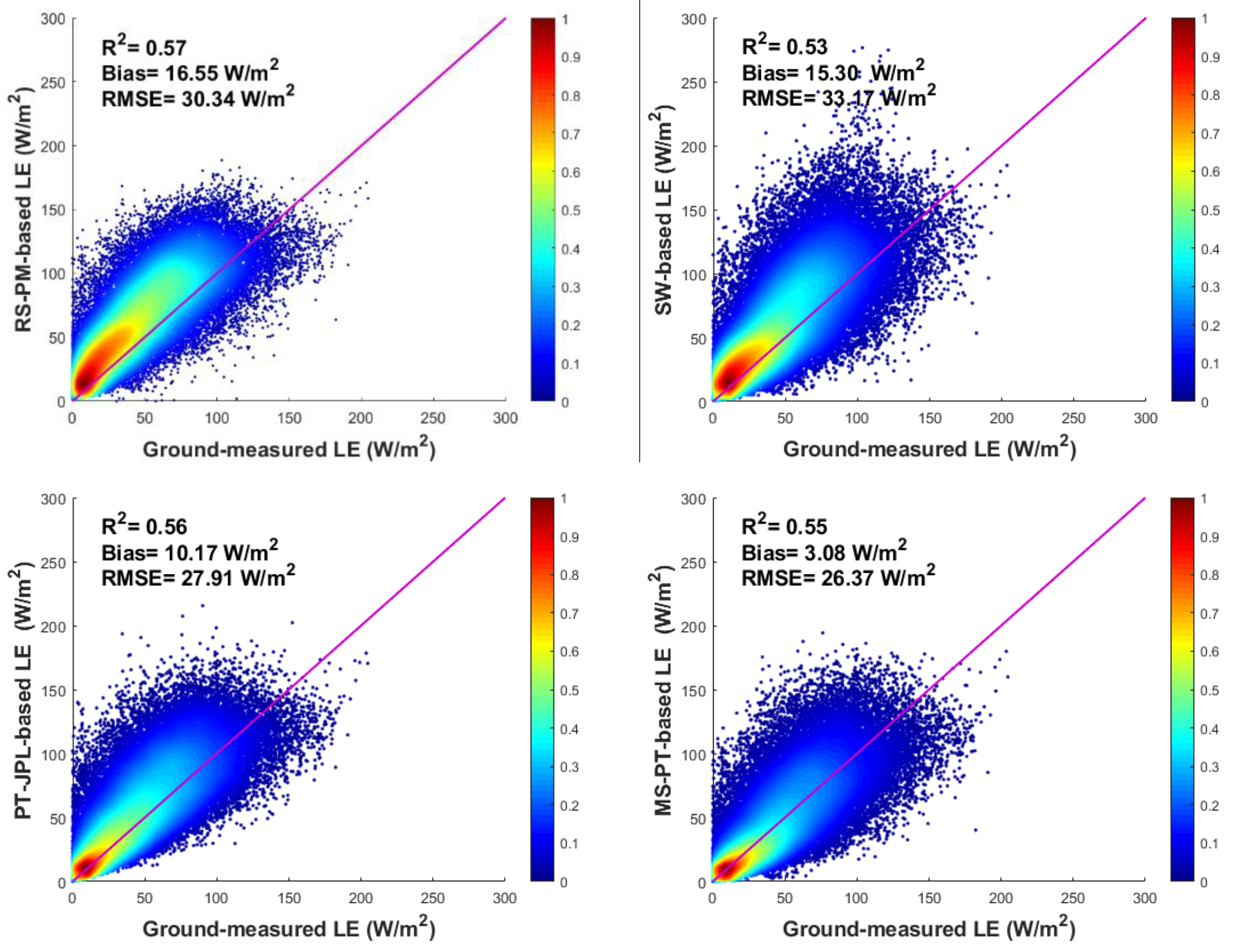
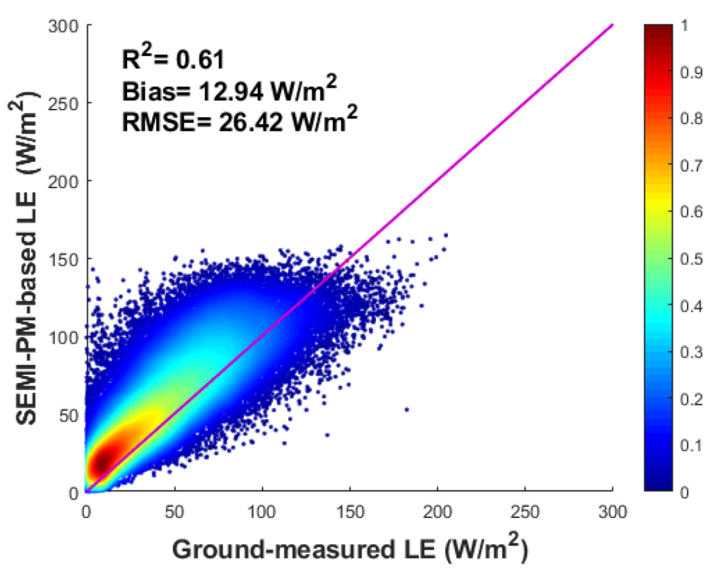
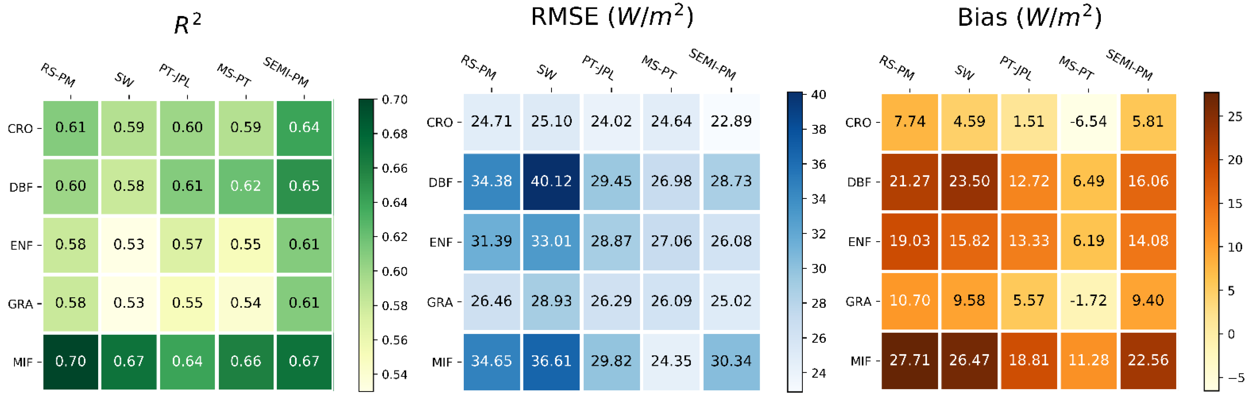
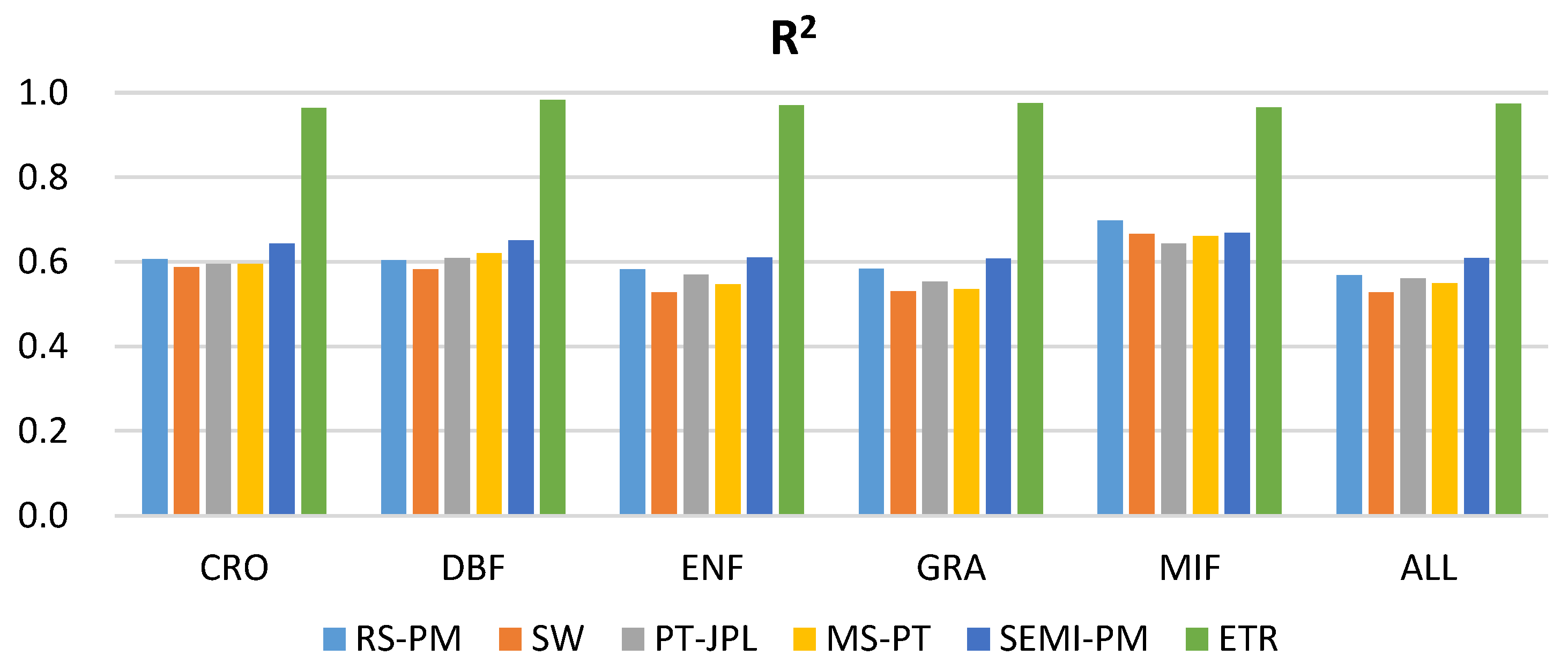
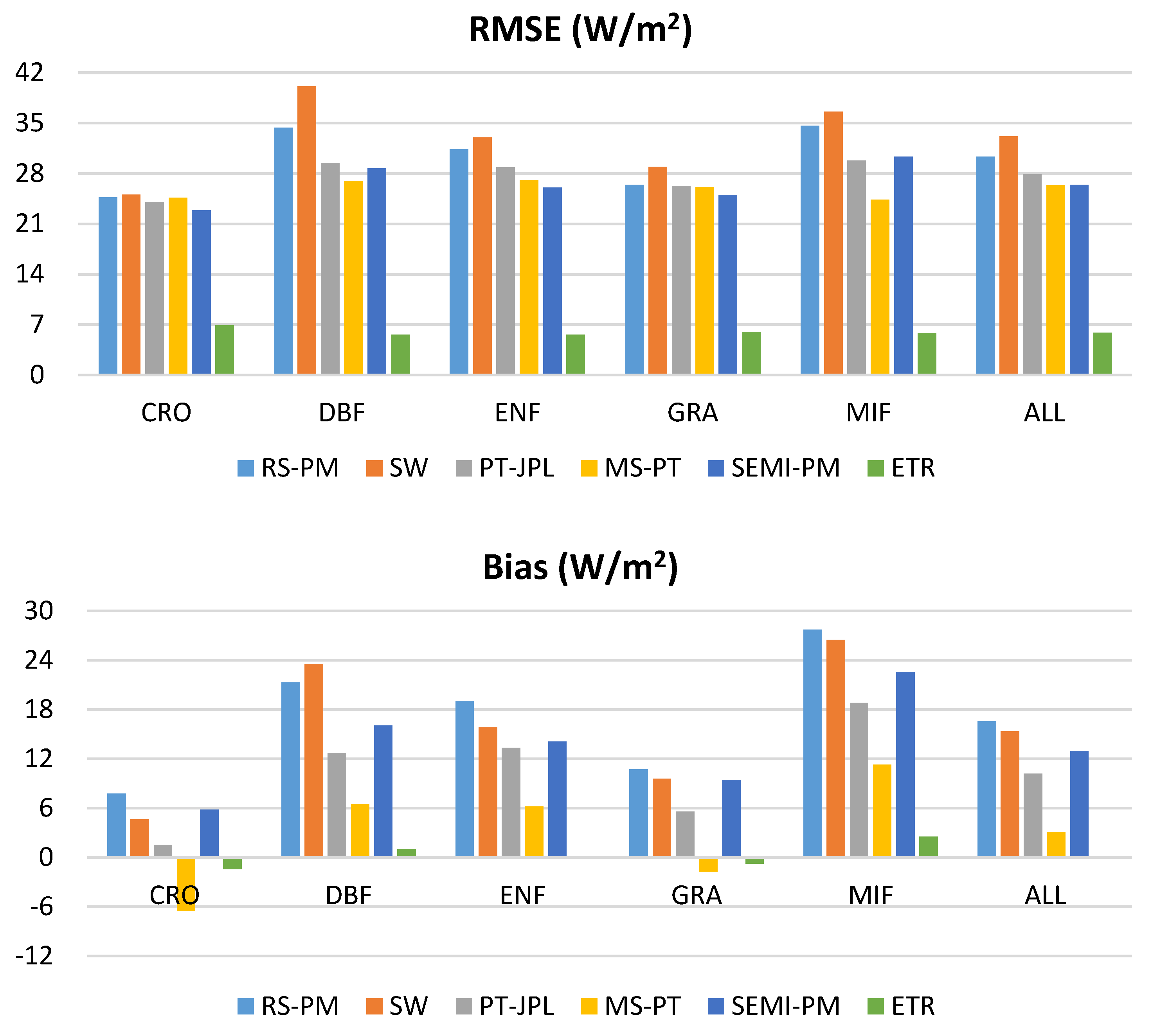
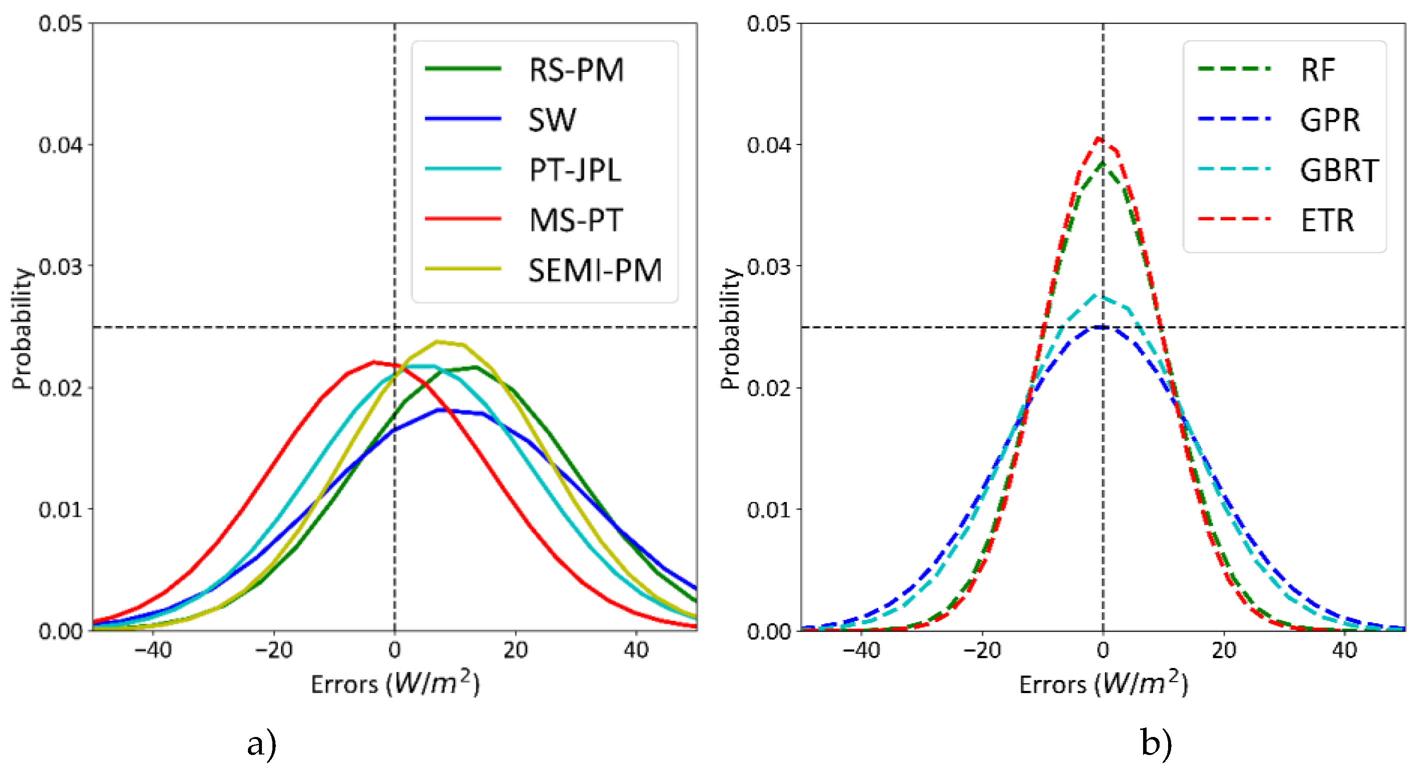
4.1. Evaluation of Satellite-Derived Terrestrial LE Products

To evaluate the five satellite-derived LE products, the corresponding estimates extracted from the individual products were directly compared with ground measurements from the 76 EC flux tower sites. Figure 2 shows the scatter plots for the daily LE observations and estimates of different LE products. The results show that the SEMI-PM product demonstrated the best performance with the highest R2 (0.61) and a small RMSE (26.42 W/m2) among the five LE products. The R2 of the SW is the smallest at 0.53, and the R2 of three other LE products vary from 0.55 to 0.57. The MS-PT obtained the smallest RMSE of 26.37 W/m2; the ascending RMSE order of the four other algorithms is SEMI-PM (26.42 W/m2), PT-JPL (27.91 W/m2) RS-PM (30.34 W/m2), and SW (33.17 W/m2).
The five LE products showed large discrepancies and uncertainties for different PFTs. Figure 3 shows the statistical summary of the evaluation parameters of the five satellite-derived products for each PFT. The results show that the MIF sites have the highest R2 which varies from 0.64 to 0.70, and the CRO sites have the smallest RMSE (22.89 W/m2 to 25.10 W/m2) and Bias (-6.54 W/m2 to 7.74 W/m2) for the different LE products. For the CRO, ENF, and GRA sites, the SEMI-PM performs better with the highest R2 (0.61 to 0.64) and the smallest RMSE (22.89 to 26.08 W/m2). For the DBF and MIF sites, the MS-PT performs better with a high R2 (0.62 to 0.66) and the smallest RMSE (26.98 and 24.35 W/m2) compared with other four LE products.
The results show that the accuracies of each LE product for different PFTs vary greatly and there are significant uncertainties between individual LE products. Moreover, we found that none of the individual satellite-derived terrestrial LE products can provide the most accurate LE estimates for all PFTs.

4.2. Fusion of Five Satellite-Derived Terrestrial LE Products Using Extremely Randomized Trees

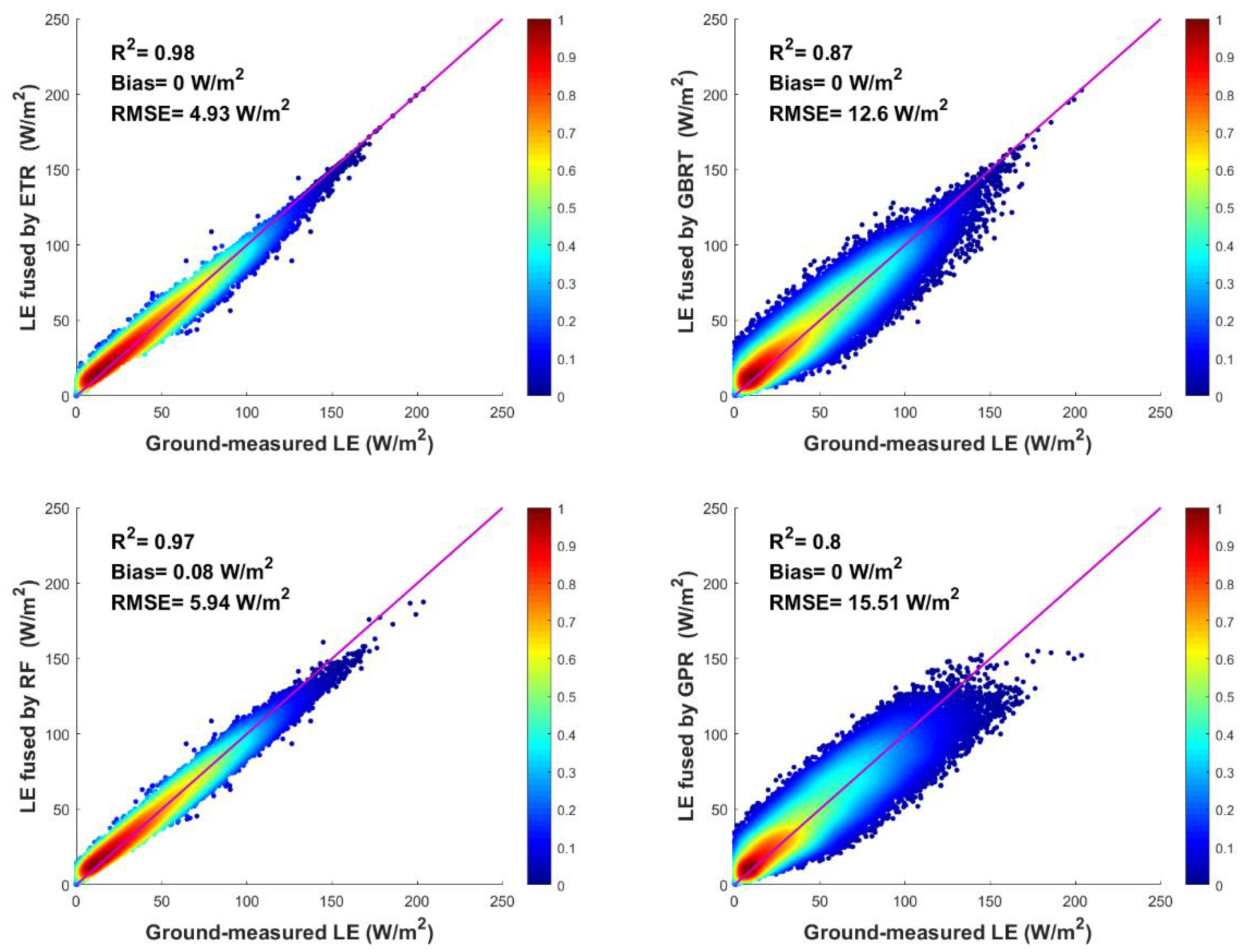
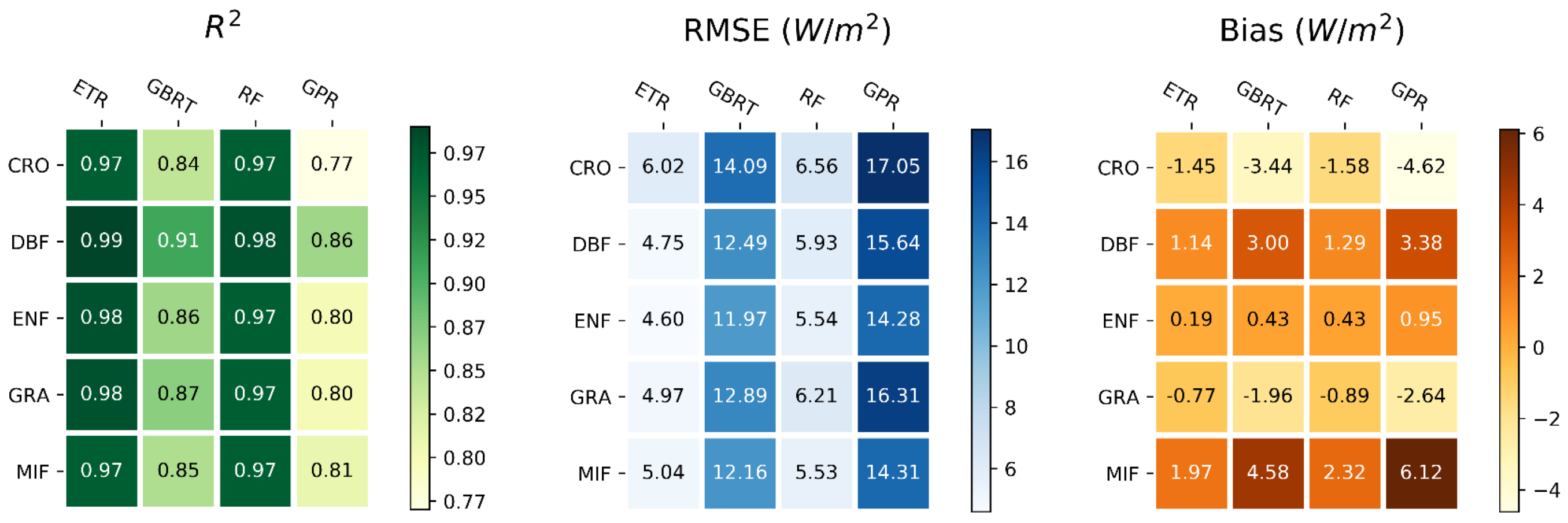
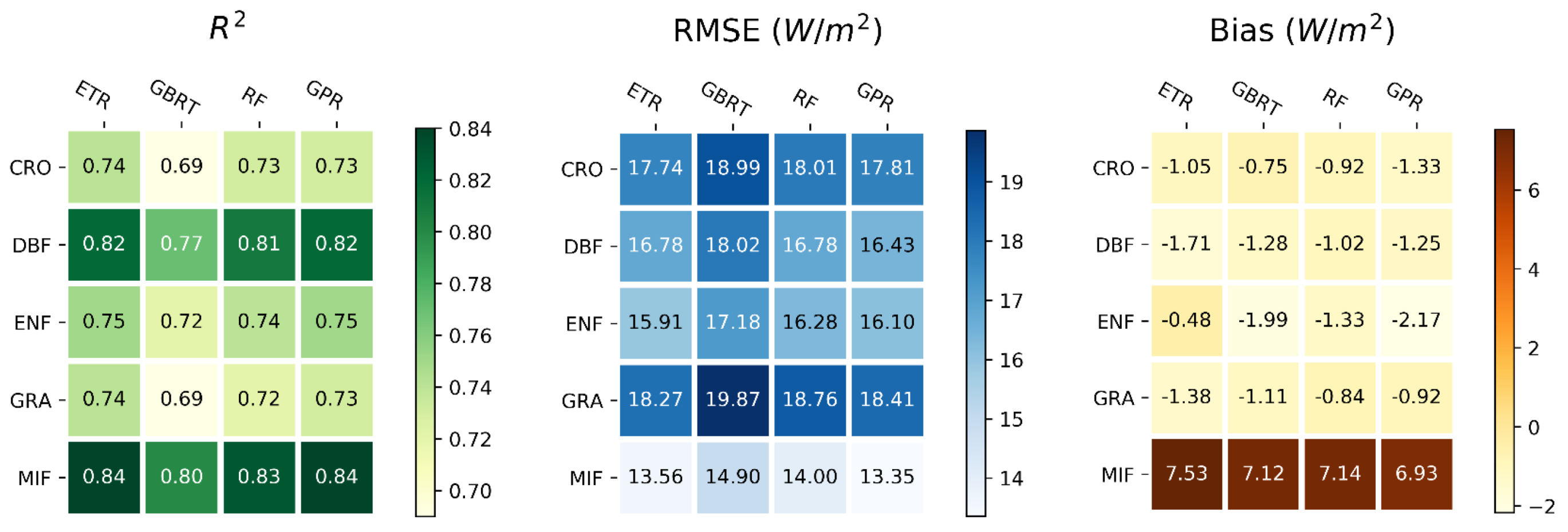
4.2.1. Model Development Using 39 Training Flux Tower Sites

To implement the fusion of five satellite-derived LE products using ETR and other three machine learning methods, the ground measurements collected at the 39 training sites were used to train the models. Figure 4 presents the scatter plots for the observations and LE training results using ETR and three other fusion models. ETR yields the best training performance with the highest R2 of 0.98 and the lowest RMSE of 4.93 W/m2 among the four fusion methods, followed by RF with an R2 of 0.97 and RMSE of 5.94 W/m2. The descending training performance order of the four algorithms is ETR, RT, GBRT, and GPR.
Figure 5 presents the statistical summary of the evaluation parameters of the four fusion methods at the 39 training sites for each PFT. One can notice that the fusion estimates using ETR for different PFTs have the highest R2 and lowest RMSE compared to the three other methods. For all the PFTs of the 39 training sites, the performance of the RF method is lower than ETR, but behaves better than the other two models, and GPR yields the lowest simulation accuracy.

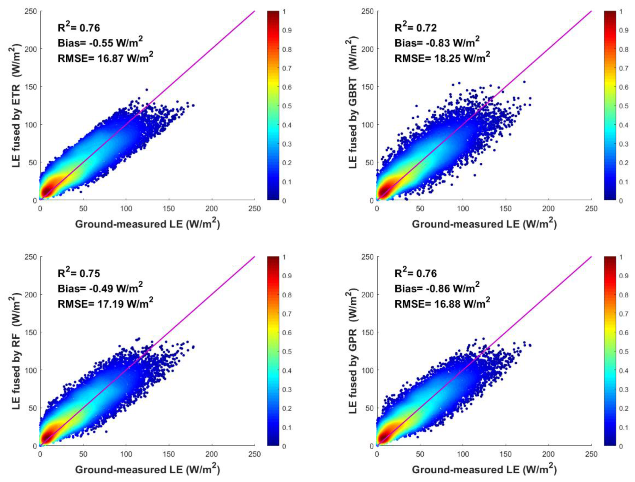
4.2.2. Model Evaluation against 37 Validation Flux Tower Sites

Figure 6 presents the scatter plots for the LE observations at the 37 validation sites and the LE inversion results using ETR and the three other fusion models. The results show that ETR yields the best training performance with the highest R2 (0.76) and the lowest RMSE (16.87 W/m2) among the four fusion models. At the specific site scale, the performance of the ETR fusion method is significantly superior to the best performance any individual LE product (SEMI-PM with an R2 of 0.61 and RMSE of 26.42 W/m2). The accuracy of the GPR fusion method is lower than ETR but much higher than RF and GBRT with an R2 of 0.76 and RMSE of 16.88 W/m2. The GBRT yields the lowest R2 (0.72) and the highest RMSE (18.25 W/m2) compared with the three other machine learning fusion methods, but it is still superior to the best performance of any individual LE product (SEMI-PM). The results show that the machine learning fusion estimates are superior to the five individual LE products, and among the four machine learning fusion methods, the ETR exhibits the best fusion performance.
Figure 7 shows the R2, Bias, and RMSE statistics of ETR and the three other fusion models for different PFTs at the 37 validation sites. Overall, whether it is R2 (varying from 0.74 to 0.84), Bias (varying from -1.71 to 7.53 W/m2), or RMSE (varying from 13.56 to 18.27 W/m2), ETR is superior to the other three fusion models at most PFTs. The performance of the GPR method is lower than ETR, but better than RF and GBRT. GBRT yields the lowest validation accuracy with an R2 ranging from 0.69 to 0.80, and RMSE ranging from 14.90 W/m2 to 19.87 W/m2. For all the PFTs, MIF has the highest R2 from 0.80 to 0.84 and the lowest RMSE from 13.35 to 14.90 W/m2, but yields the highest Bias, ranging from 6.93 to 7.53 W/m2. This may be affected by the original individual LE products, which have the same estimate tendency. The evaluation results of satellite-derived terrestrial LE products are shown in Figure 3. The DBF validation sites behave better than the three other PFTs with an R2 ranging from 0.77 to 0.82 and RMSE ranging from 16.43 to 18.02 W/m2. CRO, ENF, and GRA with lower R2, varying from 0.69 to 0.75 compared with other PTFs, are also superior to the individual LE products which obtained R2 varying from 0.53 to 0.64.
Overall, compared to the other three machine learning fusion methods, ETR exhibits a relatively high validation accuracy and stability. The enhanced accuracy of the ETR fusion method makes it a reasonable option for improving LE terrestrial estimates over Europe.

4.2.3. Implementation of Fusing Five LE Products Using Extremely Randomized Trees

To implement the fusion of five satellite-derived terrestrial LE products using ETR over Europe, we retrained the ETR model based on the EC ground measurements at all 76 sites from 2000 to 2006 and the corresponding LE estimates extracted from five individual LE products. Figure 8 shows the statistics (R2, RMSE, and Bias) of the comparison between multiple individual LE products and the fusion LE estimates using ETR for different PFTs. In general, whether it is the R2 (0.97), RMSE (5.85 W/m2), or the Bias (approximately equal to 0 W/m2), the fusion LE estimates are superior to the five satellite-derived terrestrial LE products. For all five PFTs, fusion LE estimates reduced the RMSE by 20.52 to 27.31 W/m2, representing 77.80% to 82.35% of the corresponding RMSE of the individual LE products. The Bias of individual LE products vary from 3.08 to 16.55 W/m2, and the fusion LE estimates reduced the Bias to about 0 W/m2. Therefore, the accuracy of the individual LE products was significantly improved by the fusion of multiple satellite-derived terrestrial LE products using the ETR method. The results showed that the ETR fusion method in this study could be implemented to generate a reasonable and stable regional terrestrial LE product.

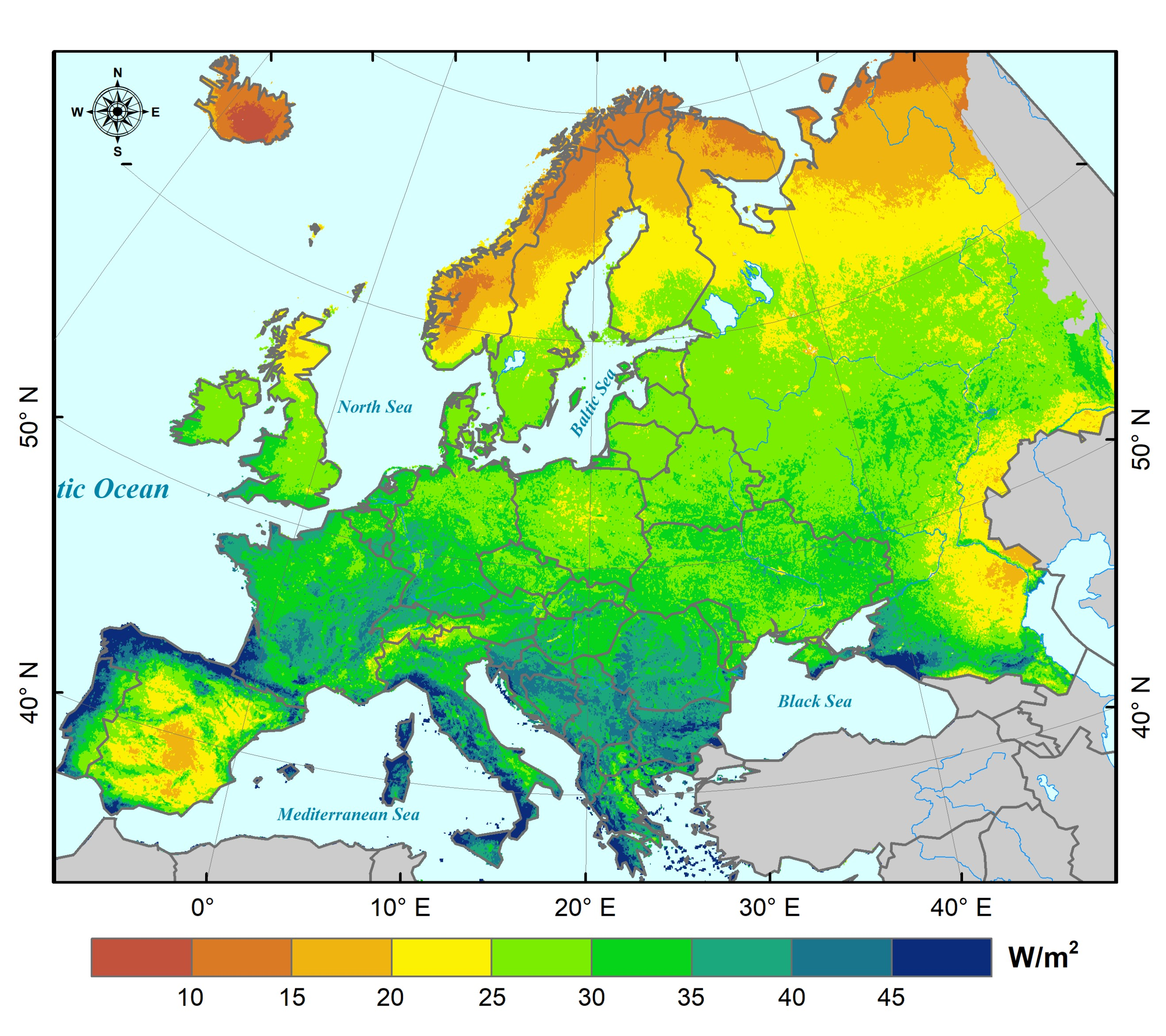
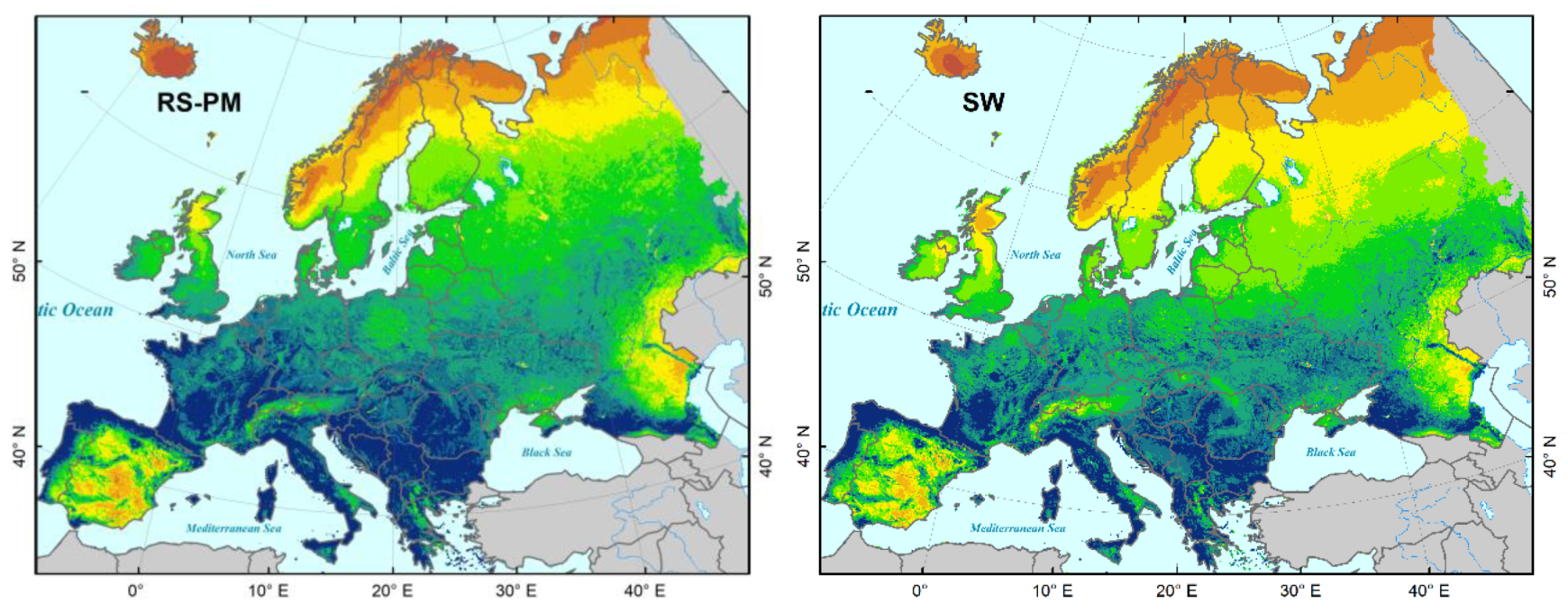
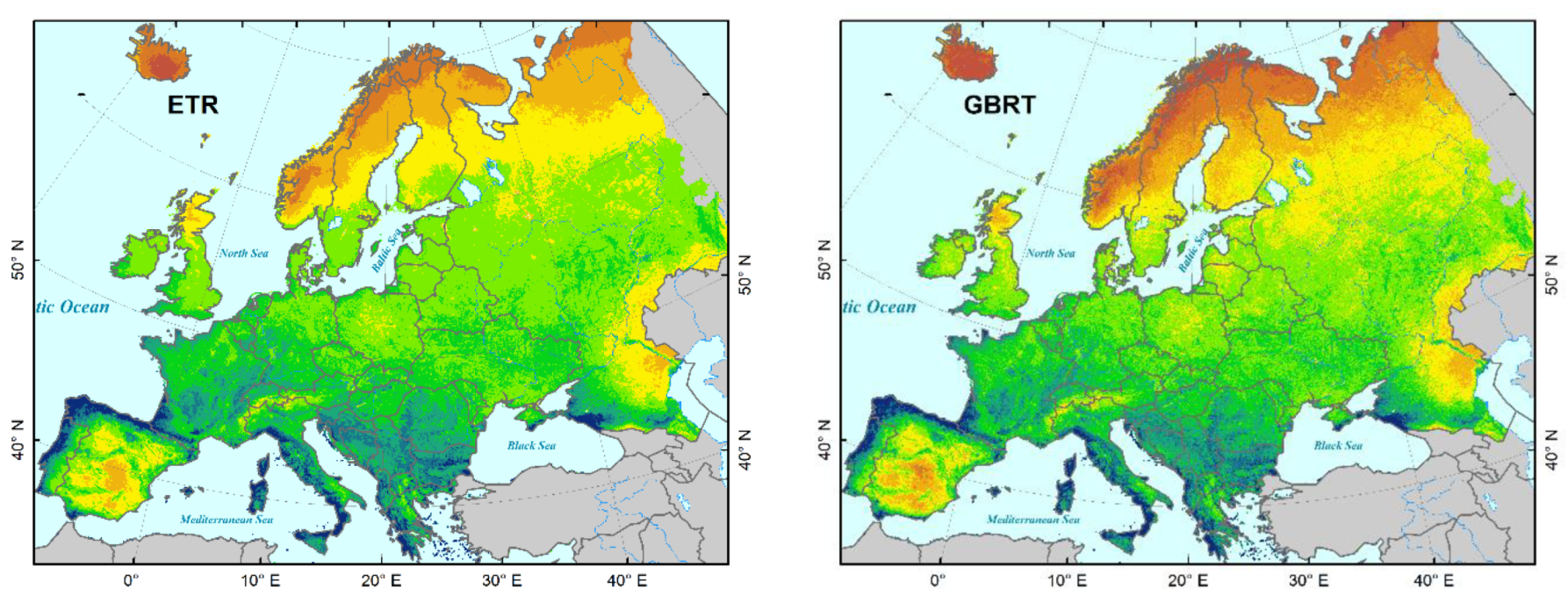
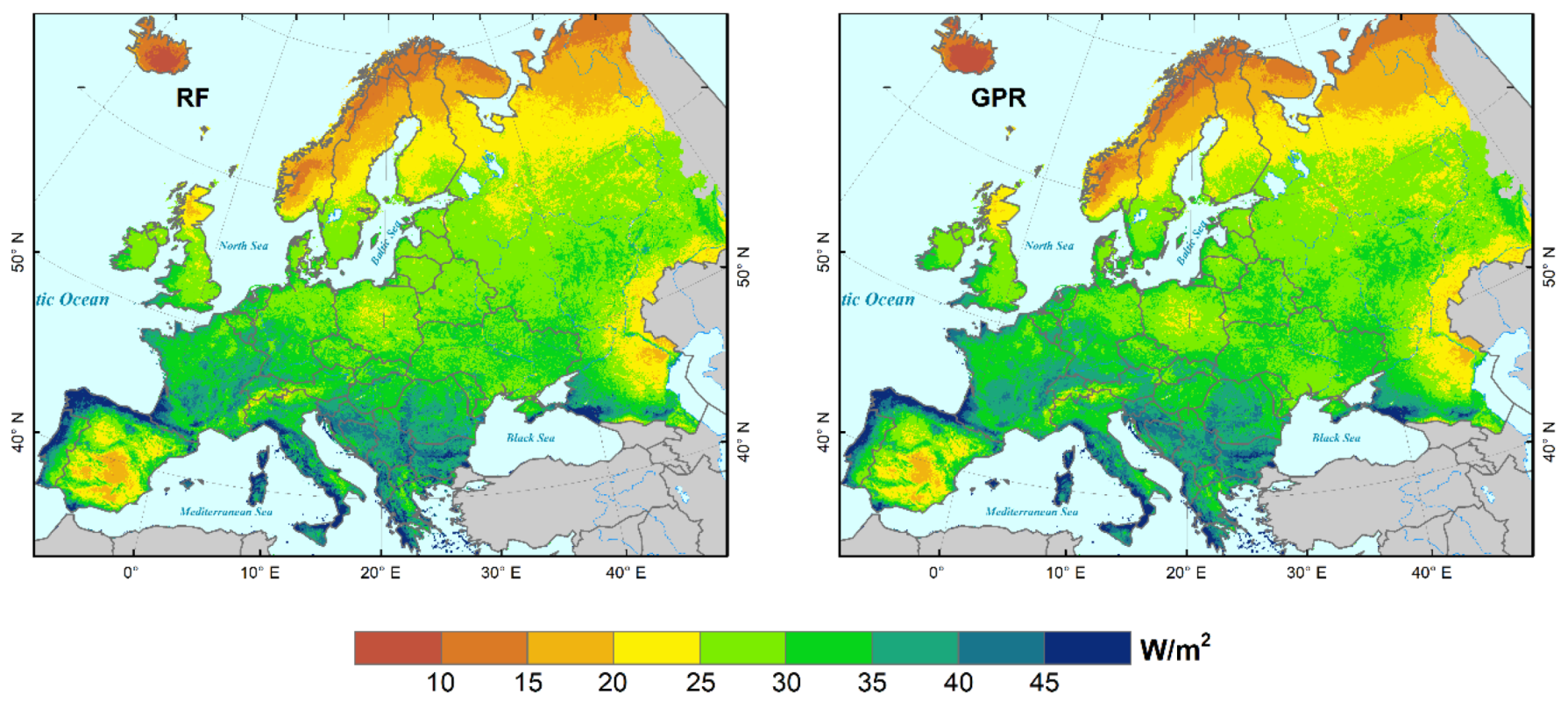
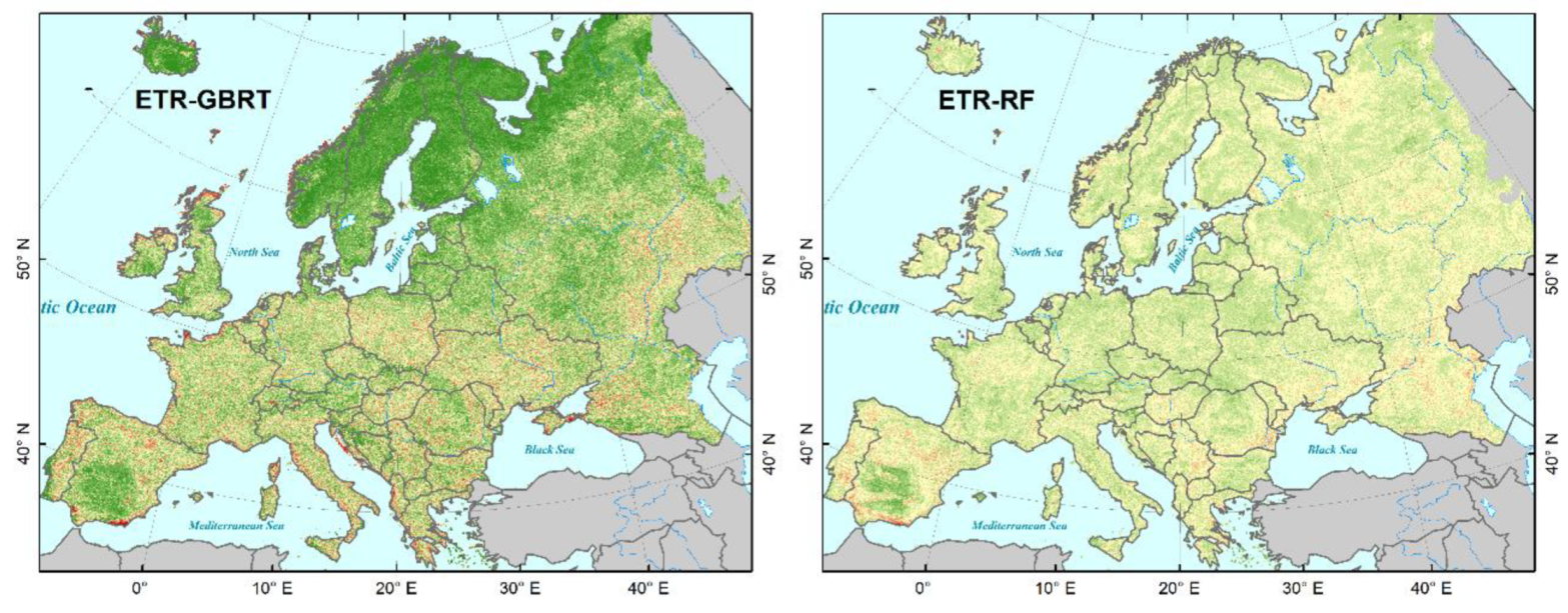
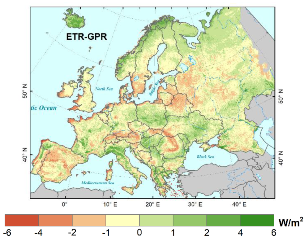
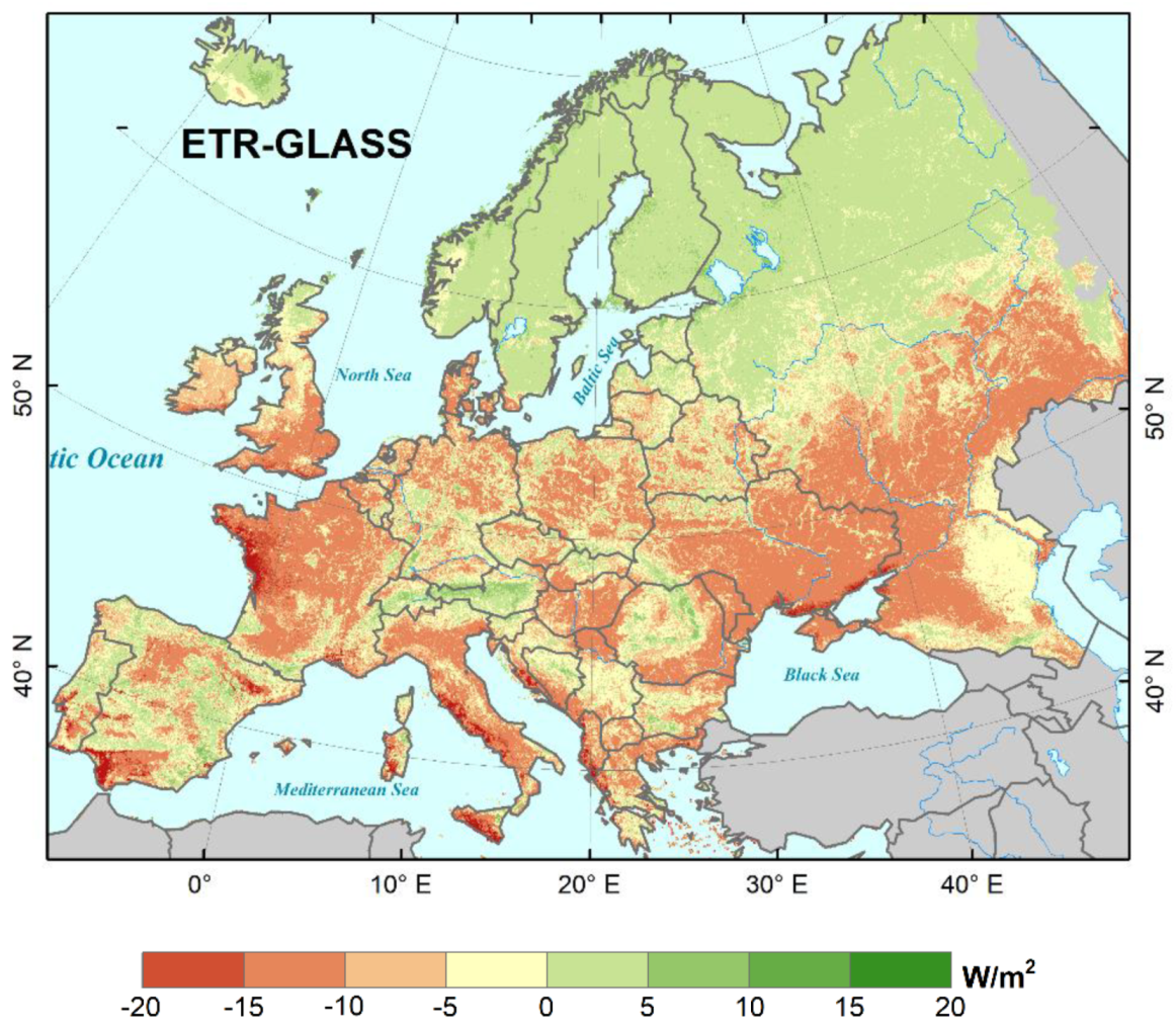
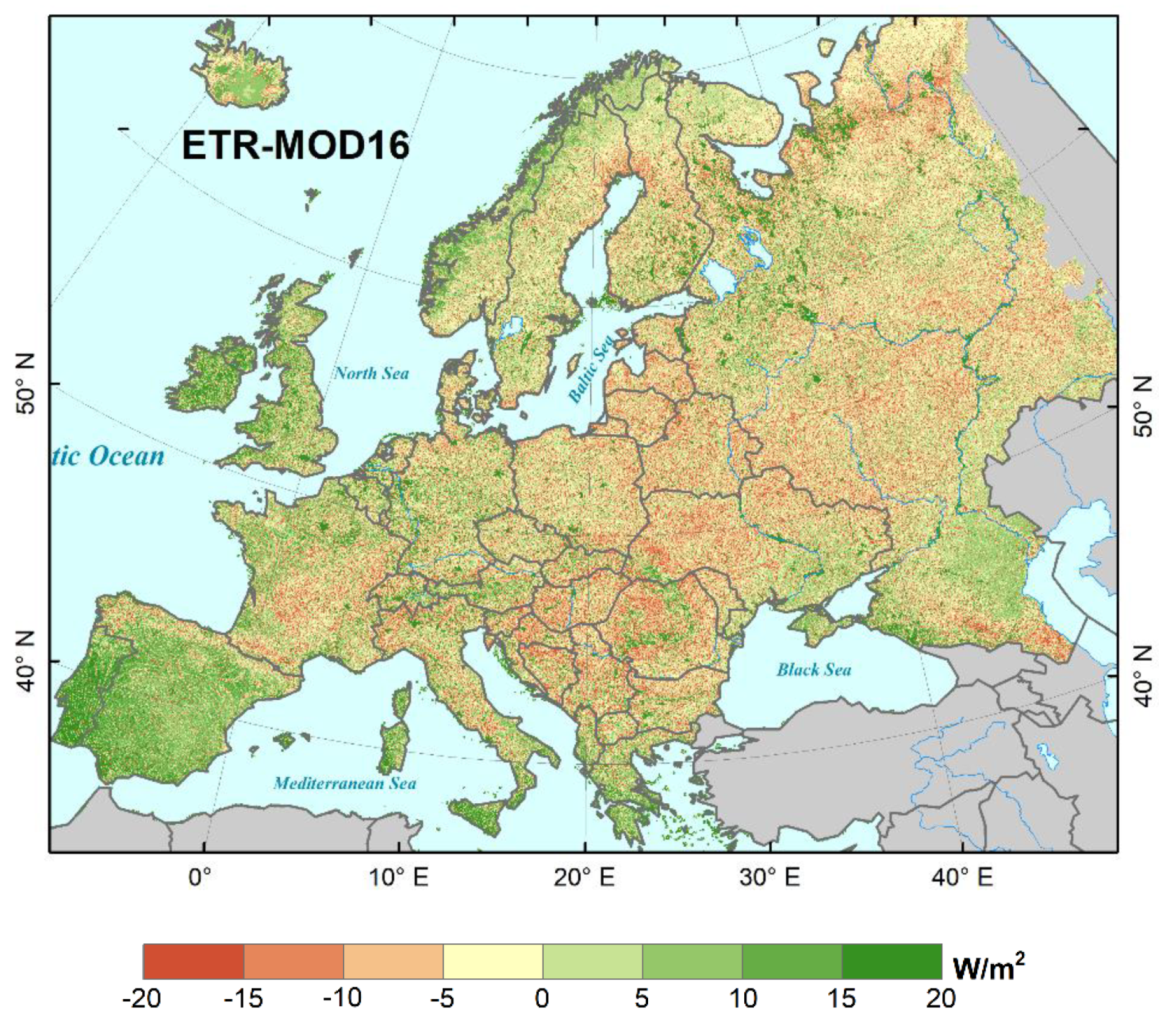
4.3. Mapping of Terrestrial LE Products over Europe

Figure 9 shows the maps of annual terrestrial LE averaged from 2002 to 2005 for the RS-PM-, SW-, PT-JPL-, MS-PT-, and SEMI-PM-based LE product over Europe. All of the five products yielded lower LE estimates over the northern portion of Europe. In the high latitudes, the highest annual LE was approximately less than 20 W/m2, appearing on the area with latitudes higher than 65°N. As the latitude decreases, LE shows a trend from low to high. The most prominent difference between the five LE products was the RS-PM- and SW-based LE products estimated higher LE values in the central and southern portions of Europe. Compared with SEMI-PM-based LE product, the PT-JPL and MS-PT yielded higher LE estimation in Austria and Bulgaria. These discrepancies maybe caused by the spatial heterogeneity and the uncertainty existing in the structures of different LE product algorithms.
We applied the fusion of five individual terrestrial LE products using ETR, GBRT, RF, and GPR to estimate the mean annual LE in the period from 2002 to 2005 with a resolution of 0.05° over Europe, respectively (Figure 10). Four fusion products showed highly consistent spatial characteristics over Europe.
When compared with the fusion terrestrial LE product using ETR, the three other fusion products generate some spatial differences (Figure 11). The GBRT yields a higher annual LE than ETR over northern Europe. As the latitude increases, the discrepancy reaches up to 6 W/m2. The fusion LE product generated by RF shows consistent spatial characteristics with ETR. The difference between the two fusion LE products was within 1 W/m2 in most parts of Europe. The GPR fusion product yields lower annual terrestrial LE in Spain, Austria, Romania, Belarus, and a higher LE in Norway, Poland, Hungary, and Italy. The difference between the two LE products was approximately within 4 W/m2 in most areas. This is possibly caused by the uncertainty existing in the structures of different machine learning fusion methods.

5. Discussion

5.1. The Performance of the Extremely Randomized Trees Fusion Method

Figure 12 shows the seasonal variation both of ground-measured LE and the estimate LE by the four fusion methods for different PFTs. For each PFT, we randomly selected a site which completely contains at least one year of ground measurements, and the corresponding estimate LE data was compared to this. The daily observed data and estimate LE were replaced by the eight-day average value. The five sites were BE-Lon (CRO), FR-Hes (DBF), DE-Har (ENF), DE-Gri (GRA), and BE-Bra (MIF).
Figure 12 illustrates that all the four machine learning fusion methods’ LE values showed great consistency with the observations for each PFT in 2005. For the DE-Har (ENF) and DE-Gri (GRA) sites, the GBRT, RF, and the GPR estimations were lower than the observations on most days of 2005. However, for the BE-Bra (MIF) and FR-Hes (DBF) sites, the three fusion models overestimated the LE with the same trend. In comparison with the GBRT, RF, and GPR methods, the seasonal LE variations generated by ETR were closest to the observations. Moreover, the RF estimate performed closely to ETR.
Of all the five sites in different PFTs, the BE-Lon (CRO) site showed a poor performance in the growing season. Studies showed that differences in crop types, and irrigation and fertilization practices may lead to noticeable influence on the accurate estimation of LE [59]. For the FR-Hes (DBF) and DE-Har (ENF) sites, a greater overlap of leaves resulting in a lower bare soil exposure ratio [60], NDVI saturates, and clouds cover [61] all contributed to the inaccurate LE estimates in these two PFTs. All four machine learning methods yielded poor performance in the BE-Bra (MIF) site, mainly because there were fewer samples available (only two sites, one for training and one for validation), which lowered the learning performance of the fusion models. In addition, all the four models presented significantly higher estimations with the same trend in BE-Bra (MIF). This may be caused by the original higher estimation of the five individual LE products at the MIF sites, which can be seen in Figure 3.
Figure 13 illustrates the probability density distributions of estimate errors in the five satellite-derived LE products and four machine learning fusion LE products, respectively. For the single LE products, the error distributions of the MS-PT are more closely centered on zero, and compared with MS-PT, the other four LE products show the same trend of overestimation. The SEMI-PM showed relatively small errors maybe because the regression coefficients of this product algorithm were calibrated using 64 global flux tower sites [47]. Overall, MS-PT and SEMI-PM yield better performance than the other products, which is also consistent with the global validation result from Yao [11].
For the fusion LE products, all the four fusion predictive errors are closely centered on zero and even the GPR method, which got the largest biases, performs better than the MS-PT and SEMI-PM. The ETR method decreased the substantial positive and negative biases. Consistent with the experiments from Geurts [50], the ETR method showed a competitive and even superior fusion performance to RF. This may be due to the ETR method having the advantage of removing the need for the optimization of the discretization thresholds which leads to its efficient implementation [45]. Therefore, the ETR strategy can accurately capture the LE variance and exhibits the best prediction performance.

5.2. Spatial Discrepancy with Global LE Products

Figure 14 shows the mean annual spatial differences between the GLASS LE product and the fusion LE estimates using ETR from 2002 to 2005. As indicated in Figure 14, relative to the GLASS LE product, the fusion result yielded lower LE (-15 ~ 10 W/m2) in most southern portions of Europe, and higher LE (0 ~ 5 W/m2) in northern Europe. This may be caused by insufficient site data and representation, as well as the characteristics of the ETR algorithm. The discrepancies between the two LE products were within 15 W/m2 in most portions of Europe.
As indicated in Figure 15, when compared with the MODIS LE product (MOD16), the fusion LE using ETR had lower estimates in central and northeast Europe and higher estimates in most parts of Spain, Portugal, United Kingdom, and Iceland. This may be caused by land surface heterogeneity and spatial continuity underrepresentation of MOD16. The difference between the two products was small and no more than 15 W/m2 in most areas.
Given the accuracy of the GLASS and MOD16 LE products, we can conclude that the fusion LE using ETR exhibits a relatively small gap compared with them, and it proved to be reasonable and reliable for the terrestrial LE estimation using the ETR fusion method over Europe.

5.3. Uncertainties of the Merged LE Estimates

Several studies have shown that the uncertainties in the MERRA meteorology data and satellite-based observations (e.g., LAI, NDVI, or FPAR), errors in tower EC observations, and mismatched spatial scales between different data sources, as well as structural differences between machine learning models all lead to the inaccuracy of LE estimates [8,9].
Firstly, studies showed that there are large biases in the MERRA data and satellite-based vegetation parameter products when validated by ground measurements at flux tower sites [62,63]. Therefore, the uncertainty of the satellite-derived LE estimates would be inherited through errors from both the MERRA and satellite-based data inputs [2]. Secondly, Foken found that large eddies cannot be measured with the EC method, which leads to the energy imbalance [48]. Although we corrected the measured LE using the method proposed by Twine [49], the corrections based on the limited understanding of the nature of the energy imbalance still result in large errors in EC measurements [64]. In addition, Hui found that gap filling of EC measurements from hourly and half-hourly data to daily averages also generates uncertainties for LE estimations [65]. Thirdly, the spatial scale mismatch among the different data sources may have introduced errors into the LE estimations. As a result of the limitation of the spatial representation of ground observation technology, no effective means exist of evaluating spatially distributed regional LE products at scales greater than a few kilometers—particularly over nonhomogeneous surfaces [66]. Finally, all machine learning methods may fall into local optimization, which results in a poor generalization performance [35]. Moreover, the fitting performance of the machine learning methods is also closely dependent on the representativeness of the training data.

6. Conclusions

We applied the Extremely Randomized Trees method to implement the fusion of five satellite-derived terrestrial LE products (RS-PM, SW, PT-JPL, MS-PT, and SEMI-PM) based on flux tower observations. By evaluating against ground measurements, we found that there are substantial uncertainty and discrepancies in the individual LE products.
On the basis of five satellite-derived terrestrial LE products, we trained and validated ETR and three other machine learning models at 76 EC flux tower sites to compare the model prediction performance. We found the ETR algorithm achieved the best fusion accuracy with the highest R2 (0.98 and 0.76) and the lowest Bias (0 W/m2 and -0.55 W/m2) and RMSE (4.93 W/m2 and 16.87 W/m2) for training and validation, respectively. Furthermore, the performance of the ETR fusion method is significantly superior to the best performance of an individual LE product at the specific site scale. When compared with moderate spatial resolution satellite-derived global LE products, such as GLASS and MOD16, the fusion LE using ETR exhibits relatively small spatial differences.
Overall, we conclude that the ETR method improved daily LE estimates over Europe by fusing five satellite-derived terrestrial LE products driven by MERRA meteorology and MODIS products. The improved accuracy of the ETR fusion method makes it a reasonable and reliable option for the estimation of terrestrial LE over Europe.

Author Contributions

K.S. and Y.Y. prepared the manuscript. Y.L., J.Y., K.J. and X.Z. revised the manuscript. X.C., X.B. and X.G. participated the discussion. All authors have read and agreed to the published version of the manuscript.

Funding

This work was partially supported by the National Key Research and Development Program of China (No. 2016YFA0600102) and the Natural Science Fund of China (No. 41671331).

Acknowledgments

We would like to thank Shaomin Liu and Tongren Xu from Faculty of Geographical Science, Beijing Normal University, China, for their suggestions to improve this manuscript. MODIS NDVI, LAI, FPAR and LE products were obtained online (https://earthdata.nasa.gov/). MERRA data were obtained online (https://disc.gsfc.nasa.gov/daac-bin/FTPSubset.pl). GLASS LAI and LE products were obtained online (http://glass-product.bnu.edu.cn/). This work used eddy covariance data were obtained from the FLUXNET community (https://fluxnet.fluxdata.org/).

Conflicts of Interest

The authors declare no conflicts of interest.

References

  1. Betts, A. Land-Surface-Atmosphere Coupling in Observations and Models. J. Adv. Model. Earth Syst. 2009, 1, 1–18. [Google Scholar] [CrossRef]
  2. Yao, Y.; Liang, S.; Li, X.; Zhang, Y.; Chen, J.; Jia, K.; Zhang, X.; Fisher, J.; Wang, X.; Zhang, L.; et al. Estimation of high-resolution terrestrial evapotranspiration from Landsat data using a simple Taylor skill fusion method. J. Hydrol. 2017, 553, 508–526. [Google Scholar] [CrossRef]
  3. Bonan, G. Ecological Climatology: Concepts and Applications; Cambridge University Press: Cambridge, UK, 2015. [Google Scholar]
  4. Jiménez, C.; Prigent, C.; Mueller, B.; Seneviratne, S.I.; McCabe, M.F.; Wood, E.F.; Rossow, W.B.; Balsamo, G.; Betts, A.; Dirmeyer, P.A.; et al. Global intercomparison of 12 land surface heat flux estimates. J. Geophys. Res. Space Phys. 2011, 116, 1–27. [Google Scholar] [CrossRef]
  5. Jimenez, C.; Martens, B.; Miralles, D.G.; Fisher, J.; Beck, H.E.; Fernández-Prieto, D. Exploring the merging of the global land evaporation WACMOS-ET products based on local tower measurements. Hydrol. Earth Syst. Sci. 2018, 22, 4513–4533. [Google Scholar] [CrossRef] [Green Version]
  6. Monteith, J.L. Evaporation and environment. In Symposia of the Society for Experimental Biology; Cambridge University Press (CUP): Cambridge, UK, 1965; pp. 205–234. [Google Scholar]
  7. Priestley, C.; Taylor, R. On the assessment of surface heat flux and evaporation using large-scale parameters. Mon. Weather Rev. 1972, 100, 81–92. [Google Scholar] [CrossRef]
  8. Mu, Q.; Heinsch, F.A.; Zhao, M.; Running, S.W. Development of a global evapotranspiration algorithm based on MODIS and global meteorology data. Remote. Sens. Environ. 2007, 111, 519–536. [Google Scholar] [CrossRef]
  9. Mu, Q.; Zhao, M.; Running, S.W. Improvements to a MODIS global terrestrial evapotranspiration algorithm. Remote. Sens. Environ. 2011, 115, 1781–1800. [Google Scholar] [CrossRef]
  10. Miralles, D.G.; Holmes, T.R.H.; De Jeu, R.A.M.; Gash, J.H.; Meesters, A.G.C.A.; Dolman, H. Global land-surface evaporation estimated from satellite-based observations. Hydrol. Earth Syst. Sci. 2011, 15, 453–469. [Google Scholar] [CrossRef] [Green Version]
  11. Yao, Y.; Liang, S.; Li, X.; Hong, Y.; Feng, F. Bayesian multi-model estimation of global terrestrial latent heat flux from eddy covariance, meteorological and satellite observations. J. Geophys. Res. Atmos. 2014, 119, 4521–4545. [Google Scholar] [CrossRef]
  12. Jiang, C.; Ryu, Y. Multi-scale evaluation of global gross primary productivity and evapotranspiration products derived from Breathing Earth System Simulator (BESS). Remote. Sens. Environ. 2016, 186, 528–547. [Google Scholar] [CrossRef]
  13. Liu, S.; Xu, Z.; Zhu, Z.; Jia, Z.; Zhu, M. Measurements of evapotranspiration from eddy-covariance systems and large aperture scintillometers in the Hai River Basin, China. J. Hydrol. 2013, 487, 24–38. [Google Scholar] [CrossRef]
  14. Liu, Z.; Shao, Q.; Liu, J. The performances of modis-gpp and -et products in china and their sensitivity to input data (fpar/lai). Remote. Sens. 2014, 7, 135–152. [Google Scholar] [CrossRef]
  15. Ruhoff, A.; Paz, A.R.; Aragão, L.E.O.C.; Mu, Q.; Malhi, Y.; Collischonn, W.; Rocha, H.R.; Running, S.W. Assessment of the MODIS global evapotranspiration algorithm using eddy covariance measurements and hydrological modelling in the Rio Grande basin. Hydrol. Sci. J. 2013, 58, 1658–1676. [Google Scholar] [CrossRef]
  16. Hu, G.; Jia, L.; Menenti, M. Comparison of MOD16 and LSA-SAF MSG evapotranspiration products over Europe for 2011. Remote. Sens. Environ. 2015, 156, 510–526. [Google Scholar] [CrossRef]
  17. A, R.; N, M.; R, M. Validation of global evapotranspiration product (mod16) using flux tower data in the african savanna, south africa. Remote. Sens. 2014, 6, 942–945. [Google Scholar]
  18. Hu, G.; Jia, L. Monitoring of Evapotranspiration in a Semi-Arid Inland River Basin by Combining Microwave and Optical Remote Sensing Observations. Remote. Sens. 2015, 7, 3056–3087. [Google Scholar] [CrossRef] [Green Version]
  19. Kumar, S.; Peters-Lidard, C.; Tian, Y.; Houser, P.; Geiger, J.; Olden, S.; Lighty, L.; Eastman, J.; Doty, B.; Dirmeyer, P.A.; et al. Land information system: An interoperable framework for high resolution land surface modeling. Environ. Model. Softw. 2006, 21, 1402–1415. [Google Scholar] [CrossRef]
  20. Rodell, M.; Houser, P.; Jambor, U.; Gottschalck, J.; Mitchell, K.; Meng, C.-J.; Arsenault, K.; Cosgrove, B.; Radakovich, J.; Bosilovich, M.; et al. The Global Land Data Assimilation System. Bull. Am. Meteorol. Soc. 2004, 85, 381–394. [Google Scholar] [CrossRef] [Green Version]
  21. Su, Z.B. A surface energy balance system (sebs) for estimation of turbulent heat fluxes from point to continental scale. Hydrol. Earth Syst. Sci. 2002, 6, 85–100. [Google Scholar] [CrossRef]
  22. Bastiaanssen, W.; Menenti, M.; Feddes, R.; Holtslag, A.A.M. A remote sensing surface energy balance algorithm for land (SEBAL). 1. Formulation. J. Hydrol. 1998, 212, 198–212. [Google Scholar] [CrossRef]
  23. Brown, K.W.; Rosenberg, N.J. A resistance model to predict evapotranspiration and its application to a sugar beet field1. Agron. J. 1973, 199–209. [Google Scholar] [CrossRef]
  24. Roerink, G.; Su, Z.; Menenti, M. S-SEBI: A simple remote sensing algorithm to estimate the surface energy balance. Phys. Chem. Earth, Part B: Hydrol. Oceans Atmosphere 2000, 25, 147–157. [Google Scholar] [CrossRef]
  25. Anderson, M.C. A Two-Source Time-Integrated Model for Estimating Surface Fluxes Using Thermal Infrared Remote Sensing. Remote. Sens. Environ. 1997, 60, 195–216. [Google Scholar] [CrossRef]
  26. Chen, Y.H.; Li, X.; Li, J.; Shi, P.; Dou, W. Estimation of daily evapotranspiration using a two-layer remote sensing model. Int. J. Remote. Sens. 2005, 1755–1762. [Google Scholar] [CrossRef]
  27. Kustas, W.P.; Norman, J.M. A two-source approach for estimating turbulent fluxes using multiple angle thermal infrared observations. Water Resour. Res. 1997, 33, 1495–1508. [Google Scholar] [CrossRef]
  28. Kustas, W.P.; Norman, J.M. Evaluation of soil and vegetation heat flux predictions using a simple two-source model with radiometric temperatures for partial canopy cover. Agric. For. Meteorol. 1999, 94, 13–29. [Google Scholar] [CrossRef]
  29. Norman, J.M.; Kustas, W.P.; Humes, K.S. A two-source approach for estimating soil and vegetation energy fluxes in observations of directional radiometric surface temperature. Agric. For. Meteorol. 1995, 77, 263–293. [Google Scholar] [CrossRef]
  30. Yao, Y.; Liang, S.; Yu, J.; Chen, J.; Liu, S.; Lin, Y.; Fisher, J.; McVicar, T.R.; Cheng, J.; Jia, K.; et al. A simple temperature domain two-source model for estimating agricultural field surface energy fluxes from Landsat images. J. Geophys. Res. Atmos. 2017, 122, 5211–5236. [Google Scholar] [CrossRef]
  31. Fisher, J.; Tu, K.P.; Baldocchi, D.D. Global estimates of the land–atmosphere water flux based on monthly AVHRR and ISLSCP-II data, validated at 16 FLUXNET sites. Remote. Sens. Environ. 2008, 112, 901–919. [Google Scholar] [CrossRef]
  32. Yao, Y.; Liang, S.; Cheng, J.; Liu, S.; Fisher, J.; Zhang, X.; Jia, K.; Zhao, X.; Qin, Q.; Zhao, B.; et al. MODIS-driven estimation of terrestrial latent heat flux in China based on a modified Priestley–Taylor algorithm. Agric. For. Meteorol. 2013, 171, 187–202. [Google Scholar] [CrossRef]
  33. Yao, Y.; Liang, S.; Li, X.; Chen, J.; Wang, K.; Jia, K.; Cheng, J.; Jiang, B.; Fisher, J.; Mu, Q.; et al. A satellite-based hybrid algorithm to determine the Priestley–Taylor parameter for global terrestrial latent heat flux estimation across multiple biomes. Remote. Sens. Environ. 2015, 165, 216–233. [Google Scholar] [CrossRef] [Green Version]
  34. Wang, K.; Dickinson, R.E. A review of global terrestrial evapotranspiration: Observation, modeling, climatology, and climatic variability. Rev. Geophys. 2012, 50. [Google Scholar] [CrossRef]
  35. Yao, Y.; Liang, S.; Li, X.; Chen, J.; Liu, S.; Jia, K.; Zhang, X.; Xiao, Z.; Fisher, J.; Mu, Q.; et al. Improving global terrestrial evapotranspiration estimation using support vector machine by integrating three process-based algorithms. Agric. For. Meteorol. 2017, 242, 55–74. [Google Scholar] [CrossRef]
  36. Li, Z.-L.; Tang, R.; Wan, Z.; Bi, Y.; Zhou, C.; Tang, B.; Yan, G.; Zhang, X. A Review of Current Methodologies for Regional Evapotranspiration Estimation from Remotely Sensed Data. Sensors 2009, 9, 3801–3853. [Google Scholar] [CrossRef] [PubMed] [Green Version]
  37. Wang, X.; Yao, Y.; Zhao, S.; Jia, K.; Zhang, X.; Zhang, Y.; Zhang, L.; Xu, J.; Chen, X. MODIS-Based Estimation of Terrestrial Latent Heat Flux over North America Using Three Machine Learning Algorithms. Remote. Sens. 2017, 9, 1326. [Google Scholar] [CrossRef] [Green Version]
  38. Bodesheim, P.; Jung, M.; Gans, F.; Mahecha, M.; Reichstein, M. Upscaled diurnal cycles of land–atmosphere fluxes: A new global half-hourly data product. Earth Syst. Sci. Data 2018, 10, 1327–1365. [Google Scholar] [CrossRef] [Green Version]
  39. Xu, T.; Guo, Z.; Liu, S.; He, X.; Meng, Y.; Xu, Z.; Xia, Y.; Xiao, J.; Zhang, Y.; Ma, Y.; et al. Evaluating Different Machine Learning Methods for Upscaling Evapotranspiration from Flux Towers to the Regional Scale. J. Geophys. Res. Atmos. 2018, 123, 8674–8690. [Google Scholar] [CrossRef]
  40. Mueller, B.; Hirschi, M.; Jimenez, C.; Ciais, P.; Dirmeyer, P.A.; Dolman, A.J.; Fisher, J.B.; Jung, M.; Ludwig, F.; Maignan, F.; et al. Benchmark products for land evapotranspiration: Landflux-eval multi-dataset synthesis. Hydrol. Earth Syst. Sci. 2013, 17, 3707–3720. [Google Scholar]
  41. Feng, F.; Li, X.; Yao, Y.; Liang, S.; Chen, J.; Zhao, X.; Jia, K.; Pinter, K.; Mccaughey, J.H. An empirical orthogonal function-based algorithm for estimating terrestrial latent heat flux from eddy covariance, meteorological and satellite observations. PLoS ONE 2016, 11, e0160150. [Google Scholar] [CrossRef]
  42. Aires, F. Combining Datasets of Satellite-Retrieved Products. Part I: Methodology and Water Budget Closure. J. Hydrometeorol. 2014, 15, 1677–1691. [Google Scholar] [CrossRef]
  43. Zhu, G.; Li, X.; Zhang, K.; Ding, Z.; Han, T.; Ma, J.; Huang, C.; He, J.; Ma, T. Multi-model ensemble prediction of terrestrial evapotranspiration across north China using Bayesian model averaging. Hydrol. Process. 2016, 30, 2861–2879. [Google Scholar] [CrossRef]
  44. Uddin, M.T.; Uddiny, M.A. Human activity recognition from wearable sensors using extremely randomized trees. In Proceedings of the 2015 International Conference on Electrical Engineering and Information Communication Technology (ICEEICT), Savar, Dhaka, 21–23 May 2015; IEEE: Piscataway, NJ, USA, 2015; pp. 1–6. [Google Scholar] [CrossRef]
  45. Geurts, P.; Louppe, G. Learning to rank with extremely randomized trees. In Proceedings of the JMLR: Workshop and Conference Proceedings, Fort Lauderdale, FL, USA, 11–13 April 2011; Volume 14, pp. 49–61. Available online: http://proceedings.mlr.press/v14/geurts11a/geurts11a.pdf (accessed on 15 January 2020).
  46. Shuttleworth, W.J.; Wallace, J. Evaporation from sparse crops-an energy combination theory. Q. J. R. Meteorol. Soc. 1985, 111, 839–855. [Google Scholar] [CrossRef]
  47. Wang, K.; Dickinson, R.E.; Wild, M.; Liang, S. Evidence for decadal variation in global terrestrial evapotranspiration between 1982 and 2002: 1. Model development. J. Geophys. Res. Space Phys. 2010, 115. [Google Scholar] [CrossRef] [Green Version]
  48. Foken, T. THE ENERGY BALANCE CLOSURE PROBLEM: AN OVERVIEW. Ecol. Appl. 2008, 18, 1351–1367. [Google Scholar] [CrossRef] [PubMed]
  49. Twine, T.; Kustas, W.; Norman, J.; Cook, D.; Houser, P.; Meyers, T.; Prueger, J.; Starks, P.; Wesely, M. Correcting eddy-covariance flux underestimates over a grassland. Agric. For. Meteorol. 2000, 103, 279–300. [Google Scholar] [CrossRef] [Green Version]
  50. Geurts, P.; Ernst, D.; Wehenkel, L. Extremely randomized trees. Mach. Learn. 2006, 63, 3–42. [Google Scholar] [CrossRef] [Green Version]
  51. Breiman, L. Random forests. Mach. Learn. 2001, 45, 5–32. [Google Scholar] [CrossRef] [Green Version]
  52. Wang, Y.; Feng, D.; Li, D.; Chen, X.; Xin, N. A mobile recommendation system based on logistic regression and gradient boosting decision trees. In Proceedings of the International Joint Conference on Neural Networks, Vancouver, BC, Canada, 24–29 July 2016. [Google Scholar] [CrossRef]
  53. Johnson, R.; Zhang, T. Learning nonlinear functions using regularized greedy forest. IEEE Trans. Pattern Anal. Mach. Intell. 2014, 36, 942–954. [Google Scholar] [CrossRef] [Green Version]
  54. Wei, Y.; Zhang, X.; Hou, N.; Zhang, W.; Jia, K.; Yao, Y. Estimation of surface downward shortwave radiation over China from AVHRR data based on four machine learning methods. Sol. Energy 2019, 177, 32–46. [Google Scholar] [CrossRef]
  55. Breiman, L. Bagging predictors. Mach. Learn. 1996, 24, 123–140. [Google Scholar] [CrossRef] [Green Version]
  56. Hesterberg, T. Bootstrap. Wiley Interdiscip. Rev. Comput. Stat. 2011, 3, 497–526. [Google Scholar] [CrossRef]
  57. Rasmussen, C.E.; Williams, C.K.I. Gaussian Processes for Machine Learning; MIT Press: Cambridge, UK, 2006. [Google Scholar]
  58. Pasolli, L.; Melgani, F.; Blanzieri, E. Gaussian Process Regression for Estimating Chlorophyll Concentration in Subsurface Waters From Remote Sensing Data. IEEE Geosci. Remote. Sens. Lett. 2010, 7, 464–468. [Google Scholar] [CrossRef]
  59. Zhang, F.; Chen, J.M.; Chen, J.; Gough, C.M.; Martin, T.A.; Dragoni, D. Evaluating spatial and temporal patterns of MODIS GPP over the conterminous U.S. against flux measurements and a process model. Remote. Sens. Environ. 2012, 124, 717–729. [Google Scholar] [CrossRef]
  60. Eugster, W.; Rouse, W.R.; Sr, R.A.P.; McFadden, J.P.; Baldocchi, D.D.; Kittel, T.; Chapin, F.S.; Liston, G.E.; Vidale, P.L.; Vaganov, E.; et al. Land-atmosphere energy exchange in Arctic tundra and boreal forest: Available data and feedbacks to climate. Glob. Chang. Boil. 2000, 6, 84–115. [Google Scholar] [CrossRef]
  61. Huete, A.; Didan, K.; Miura, T.; Rodriguez, E.; Gao, X.; Ferreira, L. Overview of the radiometric and biophysical performance of the MODIS vegetation indices. Remote. Sens. Environ. 2002, 83, 195–213. [Google Scholar] [CrossRef]
  62. Rienecker, M.M.; Suarez, M.J.; Gelaro, R.; Todling, R.; Bacmeister, J. Merra: Nasa’s modern-era retrospective analysis for research and applications. J. Clim. 2011, 24, 3624–3648. [Google Scholar] [CrossRef]
  63. Zhao, M.; Running, S.W.; Nemani, R.R. Sensitivity of Moderate Resolution Imaging Spectroradiometer (MODIS) terrestrial primary production to the accuracy of meteorological reanalyses. J. Geophys. Res. Space Phys. 2006, 111, 338–356. [Google Scholar] [CrossRef] [Green Version]
  64. Finnigan, J.J.; Clement, R.; Malhi, Y.; Leuning, R.; Cleugh, H. A Re-Evaluation of Long-Term Flux Measurement Techniques Part I: Averaging and Coordinate Rotation. Boundary-Layer Meteorol. 2003, 107, 1–48. [Google Scholar] [CrossRef]
  65. Hui, D.; Wan, S.; Su, B.; Katul, G.G.; Monson, R.; Luo, Y. Gap-filling missing data in eddy covariance measurements using multiple imputation (MI) for annual estimations. Agric. For. Meteorol. 2004, 121, 93–111. [Google Scholar] [CrossRef]
  66. Kalma, J.D.; McVicar, T.R.; McCabe, M.F. Estimating Land Surface Evaporation: A Review of Methods Using Remotely Sensed Surface Temperature Data. Surv. Geophys. 2008, 29, 421–469. [Google Scholar] [CrossRef]
Figure 1. Distribution of the 76 FLUXNET eddy covariance (EC) sites for different terrestrial biomes over Europe. The “Train” represents the training sites and the “Test” represents the validation sites.
Remotesensing 12 00687 g001
Figure 2. The scatter plots for daily LE observations at 76 flux tower sites and the estimates from the five LE products during the period from 2000 to 2006.
Remotesensing 12 00687 g002aRemotesensing 12 00687 g002b
Figure 3. The evaluation parameters (R2, RMSE, and Bias) comparison between the five satellite-derived LE products for different plant function types (PFTs).
Remotesensing 12 00687 g003
Figure 4. The scatter plots for daily LE observations at 39 training flux tower sites and LE estimates from the four fusion models during the period from 2000 to 2006.
Remotesensing 12 00687 g004
Figure 5. The evaluation parameters (R2, RMSE, and Bias) comparison between the four LE fusion methods at 39 training tower sites for different PFTs.
Remotesensing 12 00687 g005
Figure 6. The scatter plots for daily LE observations at 37 validation flux tower sites and the LE estimates from the four fusion models during the period from 2000 to 2006.
Remotesensing 12 00687 g006
Figure 7. The evaluation parameters (R2, RMSE, and Bias) comparison between the four LE fusion methods at 37 validation tower sites for different PFTs.
Remotesensing 12 00687 g007
Figure 8. The comparison of evaluation parameters (R2, RMSE, and Bias) for the five individual LE products and fusion LE estimates using Extremely Randomized Trees (ETR) for different PFTs.
Remotesensing 12 00687 g008aRemotesensing 12 00687 g008b
Figure 9. Maps of average annual terrestrial LE in the period from 2002 to 2005 for Revised remote sensing-based Penman LE product (RS-PM), Shuttleworth–Wallace dual-source-based LE product (SW), Priestley–Taylor of the Jet Propulsion Laboratory-based LE product (PT-JPL), Modified satellite-based Priestley–Taylor LE product (MS-PT), and Semi-empirical Penman-based LE product (SEMI-PM) with a resolution of 0.05° over Europe.
Remotesensing 12 00687 g009aRemotesensing 12 00687 g009b
Figure 10. Maps of average annual terrestrial LE in the period from 2002 to 2005 using the Extremely Randomized Trees (ETR), Gradient Boosting Regression Tree (GBRT), Random Forest (RF), and Gaussian Process Regression (GPR) fusion methods with a resolution of 0.05° over Europe.
Remotesensing 12 00687 g010aRemotesensing 12 00687 g010b
Figure 11. Maps of spatial difference in the annual LE average between ETR and the three other fusion methods over Europe from 2002 to 2005.
Remotesensing 12 00687 g011aRemotesensing 12 00687 g011b
Figure 12. Comparison of LE seasonal variations between estimates by the four fusion methods and ground-measures for different PFTs in 2005.
Remotesensing 12 00687 g012
Figure 13. Probability density distributions of the predictive errors in a) five satellite-derived LE product algorithms and b) four machine learning fusion methods, respectively.
Remotesensing 12 00687 g013
Figure 14. Maps of the spatial difference in the annual LE average between the Global Land Surface Satellite (GLASS) LE product and LE estimates using ETR over Europe from 2002 to 2005.
Remotesensing 12 00687 g014
Figure 15. Maps of the spatial difference in the annual LE average between the Moderate Resolution Imaging Spectroradiometer LE product (MOD16) and LE estimates using ETR over Europe from 2002 to 2005.
Remotesensing 12 00687 g015
Table 1. Summary of the five satellite-derived terrestrial latent heat flux (LE) products in this study for 2000–2006.
IDLE Product AlgorithmsSpatial ResolutionTemporal ResolutionForcing InputsReferences
1Revised remote sensing-based Penman LE product (RS-PM)0.05 degreesDailyRn, Ta, Tmin, RH, FPAR, LAIMu et al. (2011)
2Shuttleworth–Wallace dual-source-based LE product (SW)0.05 degreesDailyRn, Ta, RH, WS, LAIShuttleworth and Wallace (1985)
3Priestley–Taylor of the Jet Propulsion Laboratory-based LE product (PT-JPL)0.05 degreesDailyRn, Ta, Tmax, RH, FPAR, NDVI, LAIFisher et al. (2008)
4Modified satellite-based Priestley–Taylor LE product (MS-PT)0.05 degreesDailyRn, Ta, Tmax, Tmin, NDVIYao et al. (2013)
5Semi-empirical Penman-based LE product (SEMI-PM)0.05 degreesDailyRs, Ta, RH, WS, NDVIWang et al. (2010a)

