Radiometric Cross Calibration and Validation Using 4 Angle BRDF Model between Landsat 8 and Sentinel 2A


1
Geospatial Engineer, Advanced Remote Sensing, Sioux Falls, SD 57107, USA
2
Image Processing Lab, Engineering Office of Research, South Dakota State University (SDSU), Brookings, SD 57007, USA
3
Department of Electrical Engineering and Computer Science, South Dakota State University (SDSU), Brookings, SD 57007, USA
*
Author to whom correspondence should be addressed.
Remote Sens. 2020, 12(5), 806; https://0-doi-org.brum.beds.ac.uk/10.3390/rs12050806
Submission received: 15 January 2020
/
Revised: 15 February 2020
/
Accepted: 21 February 2020
/
Published: 2 March 2020
(This article belongs to the Special Issue Cross-Calibration and Interoperability of Remote Sensing Instruments)
Abstract
:This work describes a proposed radiometric cross calibration between the Landsat 8 Operational Land Imager (OLI) and Sentinel 2A Multispectral Instrument (MSI) sensors. The cross-calibration procedure involves (i) correction of the MSI data to account for spectral band differences with OLI and (ii) normalization of Bidirectional Reflectance Distribution Function (BRDF) effects in the data from both sensors using a new model accounting for the view zenith/azimuth angles in addition to the solar zenith/view angles. Following application of the spectral and BRDF normalization, standard least-squares linear regression is used to determine the cross-calibration gain and offset in each band. Uncertainties related to each step in the proposed process are determined, as is the overall uncertainty associated with the complete processing sequence. Validation of the proposed cross-calibration gains and offsets is performed on image data acquired over the Algodones Dunes site. The results of this work indicate that the blue band has the most significant offset, requiring use of the estimated cross-calibration offset in addition to the estimated gain. The highest difference was observed in the blue and red bands, which are 2.6% and 1.4%, respectively, while other bands shows no significant difference. Overall, the net uncertainty in the proposed process was estimated to be on the order of 6.76%, with the largest uncertainty component due to each sensor’s calibration uncertainty on the order of 5% and 3% for the MSI and OLI, respectively. Other significant contributions to the uncertainty include seasonal changes in solar zenith and azimuth angles, target site nonuniformity, variability in atmospheric water vapor, and/or aerosol concentration.
1. Introduction
Ensuring the quality and accuracy of an Earth-orbiting satellite sensor’s image data throughout its operating lifetime [1] requires regular monitoring of its radiometric and geometric performance. Subsequent postlaunch radiometric calibrations are performed to monitor the sensor response and to adjust the calibration coefficients accordingly. These calibrations can either be done in an absolute sense (i.e., deriving gains and offsets to convert raw pixel values to TOA (Top of Atmosphere) radiance/reflectance) or in a relative sense with respect to a well-calibrated “reference” sensor (a cross calibration). Of major concern among calibration scientists at this moment is the cross calibration of the Sentinel 2A Multispectral Instrument (MSI) and the Landsat 8 Operational Land Imager (OLI), which is widely considered to be the most accurately calibrated instrument.
Many techniques have been developed to perform cross calibration between satellite sensors, including efforts to calibrate all of the Landsat sensors to the OLI [2]. Research has focused on selection of “invariant” calibration sites, methods to adjust for differences in spectral response between sensors, and methods to model and correct for Bidirectional Reflectance Distribution Function (BRDF) and other effects due to differences in viewing geometry and illumination. A critical factor in producing a successful cross calibration involves selection of a calibration site regularly imaged by the sensors of interest. The site should be as temporally, spatially, and spectrally invariant as possible in order to more easily distinguish between potential changes to a sensor’s radiometric response and potential changes to the site’s surface and/or atmospheric characteristics. Historically, these sites have been in desert regions exhibiting a high degree of uniform surface reflectance, with minimal rainfall and cloud cover and with minimal signs of human settlement or other activities [3].
Rao and Chen (1995) used image data acquired over the southeastern portion of the Libyan desert (i) to identify rates of response degradation in the visible and NIR (Near Infrared) channels of the NOAA (National Oceanic and Atmospheric Administration) Advanced Very High Resolution Radiometer (AVHRR) and (ii) to establish “inter-satellite calibration linkages” between the NOAA 7 and 9 AVHRRs and the NOAA 9 and 11 AVHRRs [4]. Their analysis emphasized VNIR (Visible Near Infrared) and thermal image data acquired at satellite zenith angles of 14 or less and solar zenith angles of 60 or less to minimize BRDF and atmospheric effects. They validated their analysis results using image data acquired over the White Sands area in New Mexico. To develop an automated technique to find temporally and spatially stable Pseudo-Invariant Calibration Sites (PICS), Helder et al., used Landsat 5 TM (Thematic Mapper) image data. Six PICSs were found with spatial and temporal uncertainties within 2% in the VNIR region and within 2%–3% in the SWIR (Short Wave Infrared) region [3].
Cosnefroy et al. (1996) analyzed 20 desert sites in North Africa and Saudi Arabia for use in calibration of sensors (e.g., the ADEOS POLDER, SPOT-4 Vegetation, EOS MISR, Envisat MERIS, etc). Regions of 100 km × 100 km representing the sites were extracted from cloud-free Meteosat-4 image data where the spatial uncertainty and temporal uncertainties were 3% and 2%, repectively [5]. Many of these PICS are still considered to calibrate sensors from the recommendation of this research. Using image data from the Landsat 7 ETM+ (Enhanced Thematic Mapper Plus) and EO-1 Advanced Land Imager (ALI) sensors, Chander et al. (2010) identified the useable area, data availability, TOA reflectance, spatial uniformity, and spectral stability indicating the usefulness of a PICS for calibration [6]. They assessed six candidate sites (Mauritania1, Mauritania2, Algeria3, Libya1, Libya4, and Libya5), and the Committee on Earth Observation Sciences (CEOS) has since adopted them as calibration sites.
These analysis of PICS have been done to pick the appropriate PICS for this cross-calibration work. Among the twenty CEOS PICS, four of them (Libya1, Libya4, Niger2, and Sudan1) are considered in this work, as they have been used in previous calibration work by the South Dakota State University Image Processing Laboratory [7]. A new concept of extended PICS-finding methods was also developed very recently by South Dakota State University Image Processing Lab, where all of North Africa was analyzed as an extended PICS [8,9].
Two sensors imaging the same region on the Earth will measure different surface radiances and reflectances. A significant reason for this difference is due to inherent differences in their spectral responses. Correction factors applied to the uncalibrated sensor’s image data, called Spectral Band Adjustment Factors (SBAFs), can result in greater equalization of its data to the corresponding image data from the calibrated sensor. Research into the determination of SBAFs and their effects on cross calibration has been performed.
Teillet et al. (2004) considered the effects of spectral band differences on cross calibration [10]. Their analysis used image data of the Railroad Valley Playa (RRV) acquired by the ETM+, ALI, and Terra MODIS, ASTER, and MISR sensors, as their overpass times were within 45 minutes of each other; no BRDF or other corrections were applied to the data. The results of their analysis indicated that, with SBAF correction, the calibration accuracy was within 3%. Based on this analysis, they recommended, in general, that SBAFs should be used when cross calibrating between sensors. Chander et al. (2010) used an average of 108 EO-1 Hyperion hyperspectral profiles of the Libya4 PICS, acquired from 2004 to 2009, to determine an SBAF for Terra MODIS, using the ETM+ as the calibrated reference sensor [11]. Without SBAF correction, the observed Terra MODIS TOA reflectance was at least 16% greater than the corresponding ETM+ TOA reflectance in all bands. With SBAF correction, the difference was reduced to 6% or less. Greater uncertainties were found in the blue, NIR, and SWIR1 bands. In 2013, Chander et al., looked at the effect of SBAF correction derived from different hyperspectral data sources on the cross calibration of ETM+ and Terra MODIS using the Libya4 PICS as their test site [12]. Specifically, they considered Hyperion and SCIAMACHY (SCanning Imaging Absorption SpectroMeter for Atmospheric CHartographY) hyperspectral data. The Hyperion-based SBAF correction resulted in reflectance differences of approximately −5.51%, 2.04%, −0.83%, and 4.06% in the blue, green, red, and NIR bands, respectively. The differences were even lower when SCIAMACHY-based SBAF correction was used (−0.62%, 3.26%, 0.09%, and 0.93%,respectively).
When cross calibrating between sensors, it is highly desirable for them to image a region under similar viewing geometry and solar illumination conditions. Solar illumination and potential atmospheric effects can be accounted for if the sensors simultaneously (or near-simultaneously) image the region. Due to differences in sensor design and operation and depending on the imaged surface, differences in viewing geometry will likely result in the introduction of Bidirectional Reflectance Distribution Function (BRDF) effects. Research into the BRDF issue has resulted in a variety of models and correction approaches.
Liu et al. (2004) used a BRDF model based on the solar zenith angle in their cross calibration between Terra MODIS and MVIRS [13], using images acquired over the Dunhuang site in China. Their model extended the model originally developed by Roujean et al. (1992) [14], allowing consideration of solar zenith angles greater than 51. The estimated error due to BRDF effects was found to be approximately 2% to 3%.
Schlapfer et al. (2014) proposed a novel correction method for wide field-of-view (FOV) optical scanners based on the solar zenith, view zenith, and relative azimuth angles (i.e., the difference between the solar and view azimuth angles) [15]. Their method requires the image dataset to contain at least four distinct bands. It corrects surface cover-dependent BRDF effects using observed surface reflectances to “tune” the standard Ross-Thick and Li-Sparse BRDF models. Mishra et al. (2014) derived an empirical BRDF model based on the solar zenith and view zenith angles of Terra MODIS near-nadir images acquired over the Libya4 PICS [16]. Scene-center TOA reflectances from approximately 160 lifetime observations were plotted as a function of solar zenith angle for all reflective bands. As an initial “guess” for the model form, a simple linear model was fit to the data. Their final model was implemented using a linear function of solar zenith angle and a quadratic function of view zenith angle. They found that reflectance decreased due to BRDF effects, with greater decrease at longer wavelengths; consequently, the SWIR bands were found to be most affected.
Following application of SBAF and BRDF corrections, the sensors’ measured TOA reflectances can be compared more directly. As mentioned earlier, simultaneous (or near-simultaneous) images are acquired by the sensors in order to minimize atmospheric effects. The TOA reflectances of the uncalibrated sensor are typically modeled as a linear function of the calibrated sensor’s reflectances. Ideally, the plotted data lie directly on a one-to-one line, meaning that the measured reflectances from the sensors are equal. In practice, however, some residual deviation is typically observed, which represents a gain and/or offset in the uncalibrated sensor.
Lacherade et al. (2013) proposed a cross-calibration technique using processed MERIS and PARASOL image data acquired over the set of 20 CEOS desert sites and retrieved from the French remote sensing database SADE [17]. Instead of applying SBAF correction to the uncalibrated sensor data, the uncalibrated sensor’s surface reflectances were derived from interpolated and sampled TOA reflectances of the calibrated reference sensor. They tested the proposed approach on non-BRDF-corrected image data acquired over the CEOS Saharan desert sites and found an approximate 2% difference in the red and NIR bands. Differences of approximately 4% to 6% were observed in the green and blue bands, respectively.
Mishra et al. (2014) presented radiance- and reflectance-based cross calibration of Landsat 8 Operational Land Imager (OLI) and ETM+ [18]. Two independent datasets were used in the analysis:
- Simultaneous image pairs acquired at two Saharan desert locations during a two- day underfly event on March 29–30, 2013. One location was near the Libya4 PICS (WRS2 path 182, rows 42–43); the other was over the WRS2 path 198 rows 38–39.
- Time series analysis of images acquired over the Libya4 PICS
Results using both datasets indicate a cross-calibration uncertainty to within 2.5% in all bands but NIR, which had an uncertainty of 4% in both approaches. Even with the difference in NIR-band relative spectral responses (RSRs) between OLI and ETM+, the results were within the required 3% uncertainty for OLI and 5% uncertainty for ETM+.
Li et al. (2017) presented a method to cross calibrate the Sentinel 2A MSI and OLI sensors [19]. Using OLI as the calibrated sensor, they used Simultaneous Nadir Overpass (SNO) scenes acquired just east of the CEOS Algeria3 site. Their analysis included SBAF correction but no BRDF correction. Application of the relevant SBAFs resulted in agreement to within 3% in six of the eight corresponding bands. Overall, the MSI blue band appeared to be the best calibrated, approximately 0.08%. Calibration differences on the order of 0.4% were obtained for the green, red, and NIR bands: They were slightly higher in the coastal aerosol, blue, red, and SWIR1 bands; were approximately equal in the green band; were slightly lower in the SWIR2 band; and were significantly lower in the NIR and cirrus bands. All bands except the cirrus band improved the agreement to within 1%; the cirrus band agreement improved to approximately 2.5%.
The whole cross calibration should incorporate uncertainty in different steps. Combining the uncertainties in each step gives the total uncertainty of the whole process. A scientific method should always show the uncertainty of the value, so after following all the necessary steps, the uncertainty needs to be calculated.
Pinto et al. (2016) derived SBAFs for the OLI and CBERS 4 (China–Brazil Earth Resources Satellite 4) Multispectral Camera based on the corresponding Hyperion image data of the Algodones Dunes and Libya4 PICS using Monte Carlo simulations [20]. The simulation dataset was arbitrarily sampled to generate possible SBAF values, and from the sampled values, the associated uncertainties were estimated. Assuming maximum correlation, the uncertainty was as low as 0.4% in the green band for Libya 4 and as high as 0.87% in the NIR band for Algodones Dunes. Similarly, assuming minimum correlation, the uncertainty was as low as 0.48% in the red band for Libya4 and as high as 1.37% in the NIR band for Algodones Dunes.
Chander et al. (2013) considered uncertainties due to differences in spectral resolution, spectral filter shift, geometric misregistration, and differences in spatial resolution [21]. The spectral uncertainty was estimated from the available Hyperion and SCIAMACHY image data. The uncertainty due to spectral filter shift was estimated to be less than 2.5% in all bands, with the blue and green bands exhibiting the largest uncertainties. With respect to spatial misregistration, the estimated uncertainty was less than 0.35% in all bands. Finally, with respect to spatial resolution, the estimated uncertainty was on the order of 0.1% for all bands.
In a rigorous analysis using Monte Carlo and MODTRAN (MODerate resolution atmospheric TRANsmission) simulations, Gorrono et al. (2017) considered different sources of spectral, spatial, and temporal uncertainties affecting cross calibration of the Sentinel 2A MSI [22]. Their reference data source was hyperspectral data simulated for the upcoming Traceable Radiometry Underpinning Terrestrial and Helio Studies (TRUTHS) sensor. Their sites focused on the La Crau, Ascension Island, and Libya4 CEOS sites, representing grassland, oceanic, and desert landcover types, respectively; they also simulated snow cover. They estimated an overall uncertainty for an individual MSI overpass of approximately 0.4% to 0.5% in the “best” bands (i.e., VNIR) and approximately 0.4% to 0.7% in the “worst” bands (i.e., SWIR2). Averaging over multiple overpasses of a site, they estimated an overall uncertainty on the order of 0.2% for the “best” bands and approximately 0.3% to 0.7% for the “worst” bands. These estimates took into account both SBAF and BRDF correction.
This paper proposes a technique to perform reflectance-based cross calibration between the Landsat 8 Operational Land Imager (OLI) and Sentinel 2A Multispectral Instrument (MSI) sensors with a proposed BRDF model, using coincident pairs of OLI and MSI images acquired over the Libya 4, Libya 1, Niger 2, and Sudan 1 North African Pseudo-Invariant Calibration Sites (PICS). This work also uses coincident/nearly coincident OLI–MSI image pairs acquired over Lake Tahoe and a volcano near the Libya 1 PICS as dark targets in order to incorporate a wider range of TOA reflectance values. In addition to providing a reasonable cross calibration between OLI and MSI, this work contributes to the ongoing process of “harmonizing” image data from current and future sensors.
The paper is structured as follows. After a brief literature review, the methodology of the cross-calibration procedure is summarized. After that, results of the cross calibration are presented as are estimates of the associated individual and overall uncertainties. Then, an independent site is presented to validate the cross-calibration gains and biases. Finally, the Conclusion section summarizes the whole work and findings.
1.1. Satellite/Sensor Comparison
Landsat 8, part of the Landsat mission that has provided continuous global imaging of the Earth’s surface since 1972, was launched on 11 February 2013. It carries two sensors: the OLI and Thermal Infrared Sensor (TIRS). It flies at a nominal mean altitude of approximately 705 km in a nearly polar, sun-synchronous orbit that follows the Worldwide Reference System (WRS-2), allowing OLI and TIRS to image locations with latitudes between 80 N and 80 S [23] in a revisit time of 16 days [23]. Unlike the previous Landsat satellites, Landsat 8 can maneuver to allow its sensors to acquire off-nadir imaging and to acquire images of the Moon.
Sentinel 2A, part of the European Space Agency’s (ESA) Copernicus program [24], was launched on 23 June 2015. A second satellite, Sentinel 2B, was launched on 7 March 2017. Each Sentinel 2 platform carries the Multispectral Instrument (MSI), which images the Earth’s land and coastal areas at spatial, spectral, and radiometric resolutions comparable to those provided by the OLI in a revisit time of 10 days (with both Sentinel 2 satellites fully operational, the revisit time reduces to 5 days). Both Sentinel platforms fly at a mean altitude of approximately 786 km in nearly polar, sun-synchronous orbits phased 180 apart, allowing the MSIs to image locations at latitudes between 83 N and 56 S (Sections 1.5.1 and 1.5.2, Sentinel-2 Users Handbook [25]). Given Landsat 8’s revisit time of 16 days and Sentinel 2A’s revisit time of 10 days, opportunities for same-day, coincident acquisition by both sensors occur approximately every 80 days.
1.2. Spectral Response
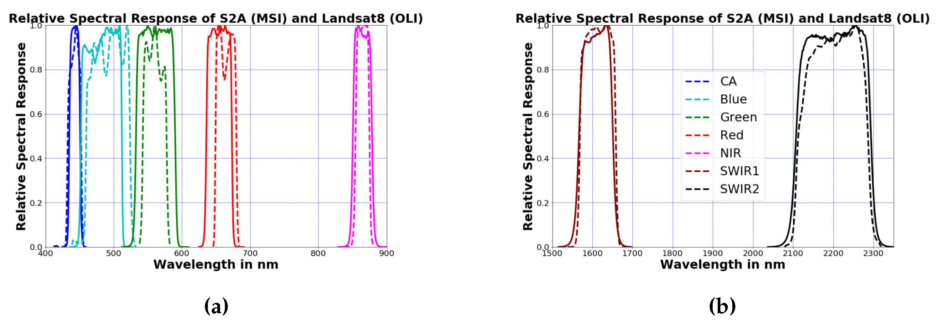
Figure 1 shows a comparison of the relative spectral response (RSR) profiles for the corresponding OLI and MSI bands [26,27]. With the exception of the blue and red bands, the difference in band centers between the two sensors is generally small. The major difference between the RSRs is that the MSI bands tend to be slightly narrower.
2. Methodology
The proposed cross-calibration process consists of the following steps. Each step is considered in greater detail in the following sections.
- Data Preprocessing and Site Selection
- Spectral Band Adjustment Factor (SBAF) Correction
- Bidirectional Reflectance Distribution Factor Normalization
- Gain and Offset Estimation
Finally, an uncertainty analysis on the estimated gains and offsets was performed. The procedure will be considered in greater detail at the end of the section.
2.1. Data Preprocessing and Site Selection
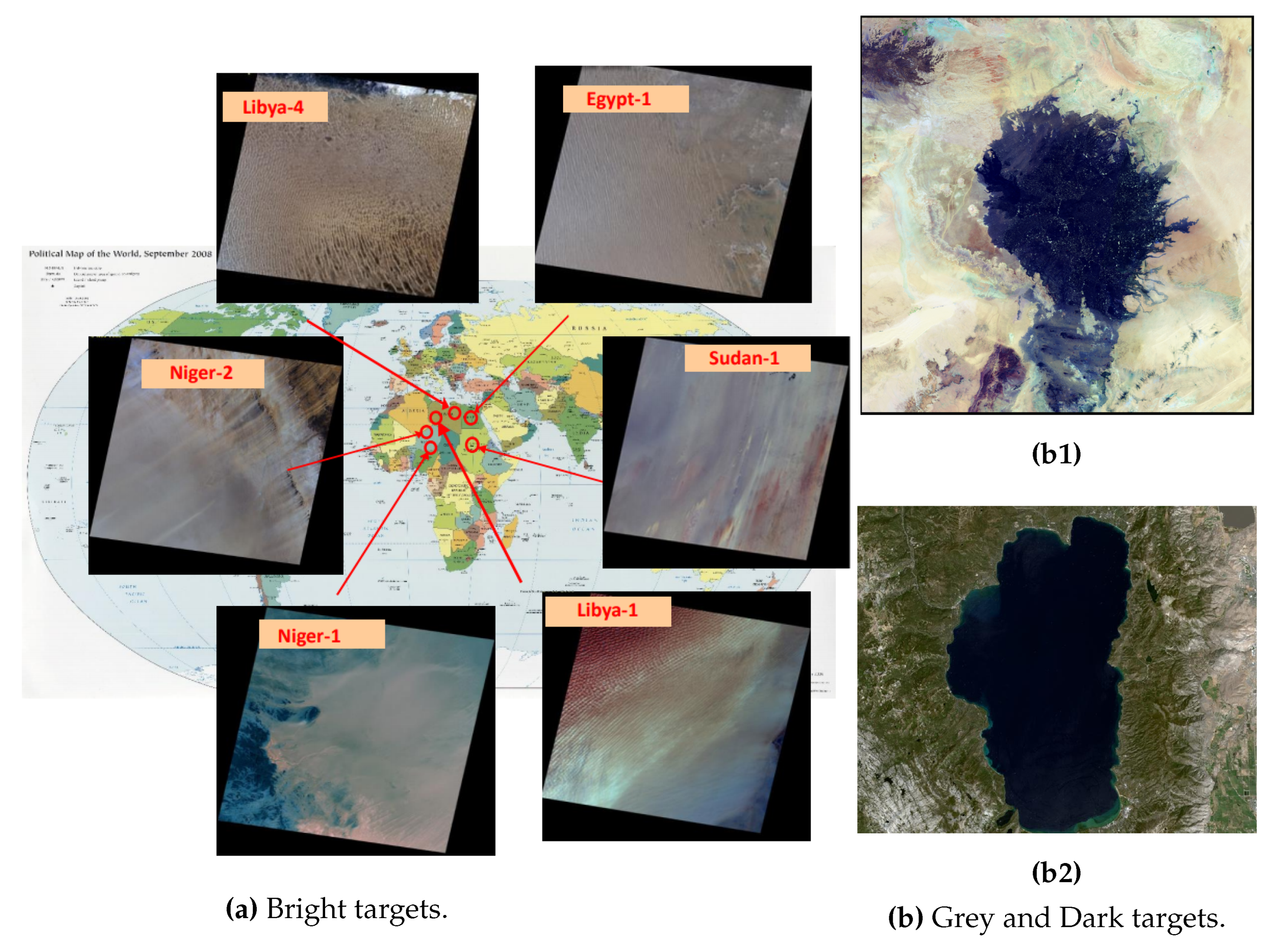
All scenes used in the analysis were initially processed by the satellite operators’ ground-processing software to correct for radiometric and geometric artifacts. The pixel values in the corrected images are 16-bit unsigned integers representing scaled TOA reflectance. For the purposes of this work, candidate target sites were those possessing up to 3% temporal and spatial scene uncertainties in all bands [28]. To allow better characterization across each sensor’s dynamic range, “bright” and “dark” target sites were considered. The bright targets consisted of rectangular regions of interest from the Libya 1, Libya 4, Niger 2, and Sudan 1 PICSs (Pseudo Invariant Calibration Sites), which have been recommended by CNES (Centre national d’études spatiales) for bright target calibration analysis [6]. These bright targets have been shown in Figure 2a.
The grey and dark targets were rectangular regions of interest extracted from a volcanic site near the Libya1 PICS (shown in Figure 2(b1)) and images of Lake Tahoe (shown in Figure 2(b2)) respectively. The ROIs (Region of Interest) from each target site were selected such that (i) the size of the region was sufficiently large (>30 km2) to minimize geometric registration errors and (ii) the ROI was identified as “optimal” with respect to minimum overall temporal, spatial, and spectral uncertainty [28]. The center latitude and longitude information is provided in Table 1 for all the target sites used in this analysis.
The set of scenes from each sensor considered for analysis was determined from a maximum estimated cloud contamination of 5%. The threshold was based on available information contained in the OLI quality band image and the MSI-associated product quality metadata. Once the appropriate target sites and ROIs were selected for both sensors, summary statistics of the TOA reflectances (i.e., mean and standard deviation) were determined for each ROI.
2.2. Spectral Band Adjustment Factor (SBAF) Correction
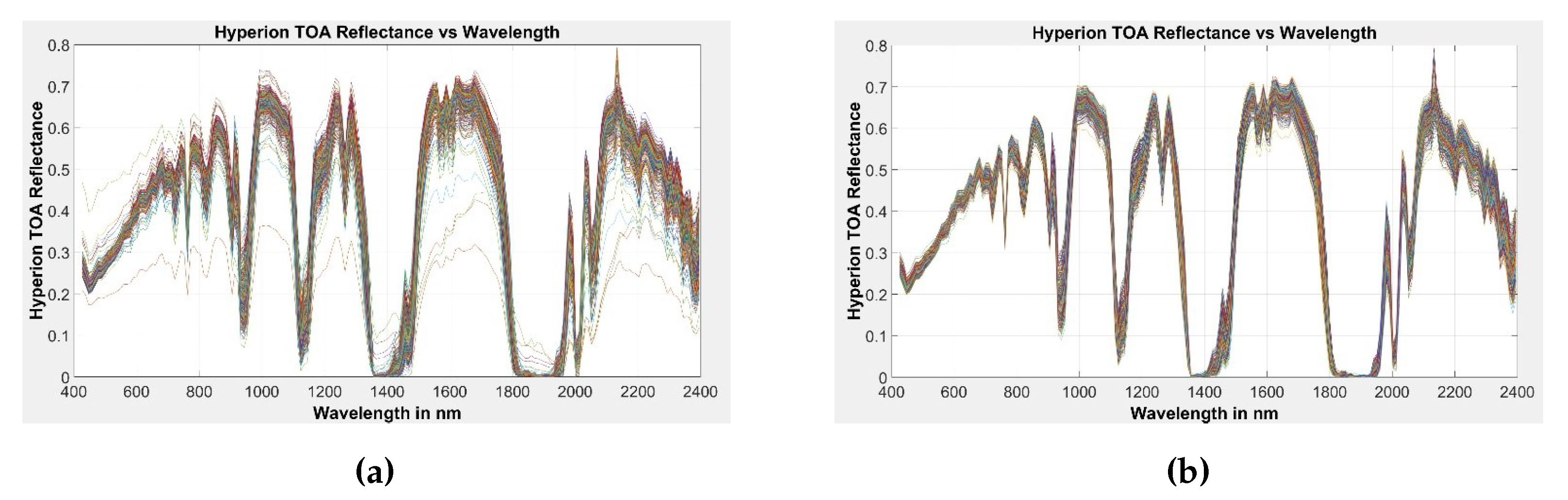
When comparing data acquired from two sensors, differences in their spectral responses, as represented by their Relative Spectral Response (RSR) functions as seen in Figure 1, must be accounted for in order to ensure a reliable analysis. Application of a Spectral Band Ajdustment Factor (SBAF) to the data from one sensor brings its response to the level of the other sensor, which is considered the “reference” with a known response. In other words, SBAF correction minimizes the effects of differences in sensor RSRs. For each scene date, the mean hyperspectral reflectance profile of the target ROI was generated from the corresponding cloud-free Hyperion image data (Figure 3a), using a threshold of around the mean TOA reflectance profile; this excluded profiles from 283 scenes potentially affected by clouds and/or shadows (Figure 3b). For each target ROI, the SBAF for each profile was calculated according to the process used by Chander et al., [11].
SBAFs relating the MSI spectral response to the OLI spectral response are calculated and applied to the MSI data. For each scene date, the mean hyperspectral reflectance profile of the target ROI is generated from the corresponding cloud-free Hyperion image data. The in-band reflectance for each sensor is calculated by integrating the portion of the hyperspectral profile contained within the sensor RSR bandwidth and then by dividing that value by the integral of the sensor RSR. The SBAF for the target is the ratio of the reference sensor in-band reflectance to the uncalibrated sensor’s in-band reflectance:
where:
| =in-band TOA reflectance of OLI (Unitless) | |
| =in-band TOA reflectance of MSI (Unitless) | |
| =hyperspectral TOA reflectance profile of the target (Unitless) | |
| =OLI relative spectral response | |
| =MSI relative spectral response |
The individual SBAFs derived for each target ROI were then averaged to obtain an overall set of site-specific SBAFs, which were then used in the final cross-calibration calculations.
Table 2 shows the calculated SBAF values and corresponding standard deviations estimated from 343 Hyperion Libya 4 scenes (available cloud-free scenes from January, 2004 to March, 2017). The blue and red bands exhibited the largest deviation in SBAF from unity (approximately 4% and 2%, respectively). The green band exhibited an approximate 0.5% deviation from unity. The coastal aerosol, NIR, SWIR1, and SWIR2 bands exhibited SBAF values very close to unity (on the order of 0.05% or less). In general, the SBAF standard deviations were larger at shorter wavelengths than at longer wavelengths. This is consistent with the greater differences in RSR bandwidth and center wavelength.
Table 3 shows a summary of the estimated SBAFs for the remaining sites. The volcano dark site shows consistent behavior with the brighter PICS in terms of SBAF values. The Lake Tahoe site tends to exhibit greater deviations from unity in the shorter wavelength bands; interestingly, its SBAF in both SWIR bands is very consistent with the corresponding volcano site SBAFs. For the remaining sites, the green band SBAF shows significant deviation from unity. From Figure 1, the blue, green, and red bands have the least agreement in RSR between the two sensors, with the OLI RSR bandwidths generally larger than the MSI bandwidths; the NIR, SWIR 1, and SWIR 2 bands have the most agreement in RSR. The calculated SBAFs were applied to the MSI’s mean TOA reflectance for each site (assuming that the OLI was the preferred reference, as its calibration is known to a high degree). After this correction, differences due to RSR response differences were reduced to around 1%. Residual differences in response due to Bidirectional Reflectance Distribution Function (BRDF) effects remained, however, and needed to be accounted for. The next section describes how these effects were considered for both sensors.
2.3. BRDF Modeling and Normalization
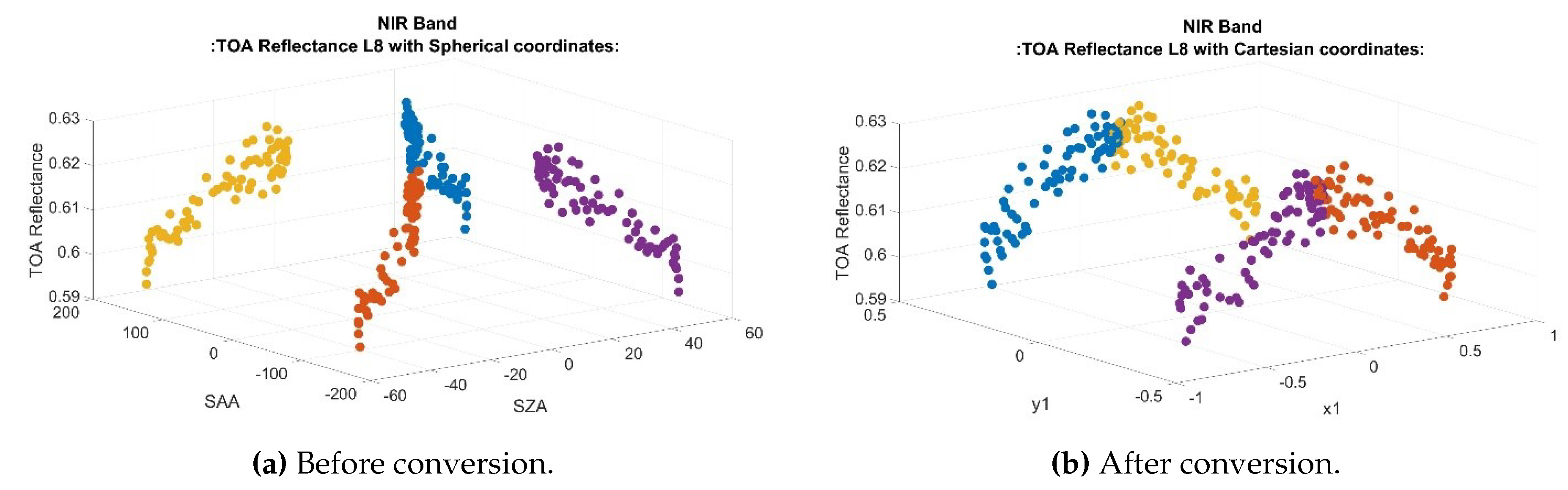
BRDF normalization in previous cross-calibration efforts has typically emphasized the solar zenith angle [16]. This section describes a four-angle, site-specific BRDF model derived for each band where the wavelength dependence is considered minimal. From the set of acquisition solar zenith/azimuth and view zenith/azimuth angles in the spherical coordinate system (designated here as SZA, SAA, VZA, and VAA), a new set of variables () were generated through transformation of the angles to plane Cartesian coordinates using Equations (2)–(5) [29].
Figure 4a shows the NIR band TOA reflectance plotted with respect to the original solar zenith and azimuth angles, with the data mirror into each quadrant. From an South Dakota State University Iplab experience, where the range and possible solar angles is not limited, practical experience tells us that the data should be asymmetric about the axis. This is needed in order to reduce the modeling errors and to reduce edge effects due to the limited operational variability in the view geometries. The next issue is the conversion of data from spherical coordinated system to Cartesian. This is a necessary step due to the modeling that is being applied to the data; modeling on an evenly spaced grid of data allows for simple mathematical models and tighter fits to the data. This can be seen by looking at Figure 4b, where, when the data is converted to Cartesian and plotted on a Cartesian coordinates, the data can be seen as continuous data.
The transformed coordinates are inputs to a multi-linear least-squares model assuming no interaction between the various angles.
Once the models were generated, “reference” solar and sensor view zenith/azimuth angles were selected by identifying a common set of solar and sensor view angles measured at all of the selected sites. A reference TOA reflectance is calculated from Equation (6) and then scaled by the ratio of the observed and model predicted TOA reflectances to obtain the TOA reflectance applicable to the site ROI as seen in SZA = 30, VZA = 0, SAA = 125, and VAA = 10:
For the cross-calibration analysis, each sensor’s TOA reflectance was normalized assuming the four-angle linear model as described in Equations (2)–(5) and (6). However, the observed TOA reflectance response in the OLI NIR band suggested quadratic behavior with respect to Cartesian coordinate x1 (i.e., sin(SZA)*sin(SAA)), as shown in Figure 4b.
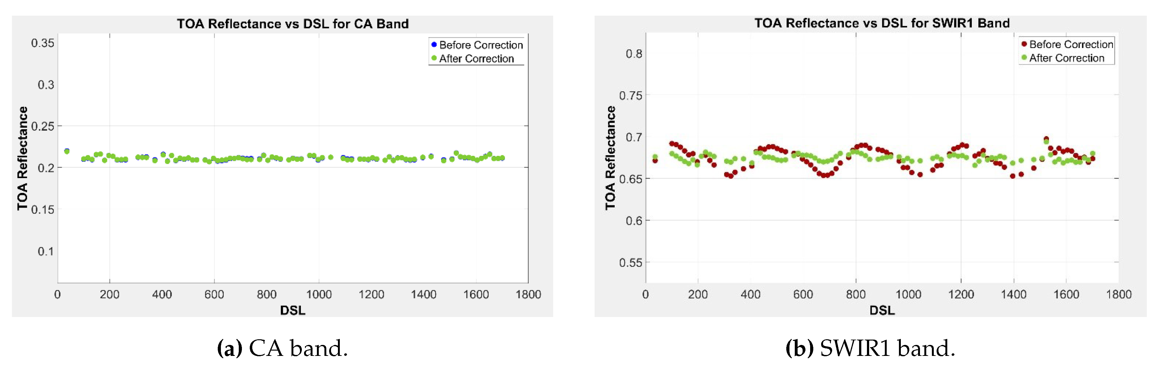
Figure 5a,b shows the amount of normalization achieved by the proposed four-angle linear BRDF model in the coastal aerosol and SWIR1 lifetime TOA reflectance trends. More normalization is evident in the SWIR1 band than in the Coastal Aerosol (CA) band. This is because of the fact that the SWIR1 band has a more pronounced seasonal effect than other bands.
To compare uncertainties relating to selection of a linear vs quadratic BRDF model, TOA reflectances normalized with the proposed four-angle linear model in Equation (6) were compared to the corresponding results obtained from (i) linear and quadratic models based on the spherical SZA alone (Figure 5a,b respectively) which is obtained from Reference [16] and (ii) a multi-linear four-angle model based on the Cartesian coordinates that accounted for second-order effects and allowed interactions between all angles as in Equation (8) and Equation (9). The BRDF-normalized TOA reflectances for all models were normalized using Equation (7). The pre- and post-normalization reflectance uncertainties associated with each model are presented in Table 4. Clearly, all models provided significant correction at longer wavelengths, as indicated by the reduction in post-normalization uncertainties. The proposed four-angle linear model provided comparable normalization to the quadratic SZA model, and both account for more BRDF effect than the linear SZA model, consistent with the quadratic characteristic shown in Figure 4b. The multi-linear four-angle interaction model provided the best BRDF model characterization and thus the best after-normalization uncertainty. At shorter wavelengths, none of the tested models provided significant (the difference between before and after normalization uncertainty is within 0.3%) BRDF normalization; the proposed four-angle model provided essentially the same reduction in uncertainty as the linear SZA model. Again, the linear four-angle interaction model provided the best BRDF characterization and normalization; the quadratic and interaction terms appear to better represent the BRDF response. For future cross-calibration analyses, the multi-linear four-angle interaction model is recommended.
One of the reasons behind why the BRDF models should account for more precise BRDF effects is that Landsat collection 1 data provides pixel-by-pixel view and solar angle information while, before providing collection 1 data, Landsat metadata only used to provide a scene center angle information. Sentinel MSI image data products also provide pixel-based angle information but at a resolution of 5000 m. To obtain more representative pixel-based angle information, the MSI angle data were resampled to a 10-m spatial resolution. Levels of BRDF normalization similar to the Landsat correction were obtained with the resampled Sentinel angle information. Once MSI and OLI data are BRDF normalized, they are ready to do a one-to-one comparison so that the level of TOA of MSI can be moved to the level of TOA of the reference sensor OLI. The following subsection discuss the process of calculation of gain and bias for the cross calibration.
2.4. Gain and Offset Calculation
Cross-calibration gains and offsets were calculated from 35 SBAF- and BRDF-corrected scene pairs from the Saharan PICS and Lake Tahoe sites. The PICS and Lake Tahoe scene pairs were effectively coincident (i.e., acquired within 30 min of each other), while the scene pairs from the Libyan volcanic site were nearly coincident (acquired within 3 days of each other). Table 5 gives the number of scene pairs selected for each target site.
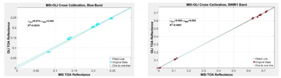
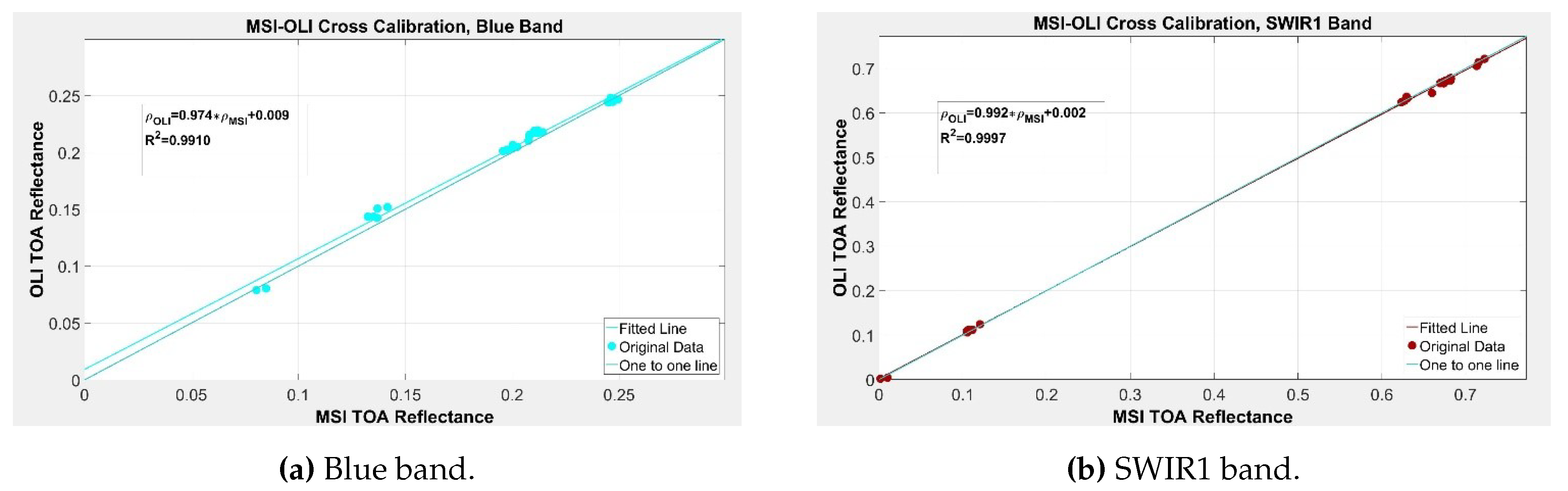
Least-squares linear regression was performed on the scene pair data to determine the cross-calibration gain and offset for each band. The regression data were plotted with the estimated regression line and a 1-to-1 line representing equality between the OLI and MSI TOA reflectances. Example plots for the blue and SWIR1 bands are shown in Figure 6. With the exception of the blue band, the estimated offsets from the 1-to-1 line were generally quite small, less than 0.002 reflectance units in magnitude. The estimated offset from the 1-to-1 line in the blue band was approximately 0.0092 reflectance units.
Table 6 presents the results of hypothesis tests on the regression slopes and intercepts (gains and offsets, respectively) at the 95% significance level. The hypothesis tested here is as follows: null hypothesis: slope = 0 and bias = 0; alternative hypothesis: slope ≠ 0 and bias ≠ 0 (forced zero regression). There is sufficient statistical evidence to conclude that the cross-calibration gains differ from 1.0 and insufficient statistical evidence to conclude that the offsets are different from 0, with the exception of the blue band, of which the estimated p-value was approximately 0.0145. As there was insufficient statistical evidence in general to justify assuming a nonzero offset, alternative regressions were performed such that the intercepts were forced to pass through 0. The slope hypothesis tests were rerun at the 95% significance level. Table 7 presents the results of the updated tests. Clearly, as noted with the full regression hypothesis tests, there is sufficient statistical evidence to conclude that the cross-calibration gains in all bands differ from 1.0.
2.5. Uncertainty Analysis
Measurement of any physical quantity has an associated level of uncertainty due to inherent variability in the measured data itself and/or uncertainties related to the techniques and equipment used to perform the measurement. For this analysis, the uncertainties in the individual sensor calibrations, RSR response, site variability, and SBAF and BRDF normalizations are the primary factors determining the overall cross-calibration uncertainty. This section describes these component uncertainties and the determination of the final cross-calibration uncertainty in greater detail.
2.5.1. Uncertainty Due to Sensor Calibration
The cross-calibration procedure described earlier depends on TOA reflectances derived from radiometrically calibrated sensor image data. Consequently, uncertainty associated with the individual sensor calibrations is a component in the final cross-calibration uncertainty. To date, the currently accepted uncertainties in the OLI and MSI calibrations are approximately 3% and 5%, respectively, as determined by the sensor vendor prelaunchs and confirmed through multiple postlaunch analyses [30].
2.5.2. Uncertainty Due to Changes in Prelaunch RSR
To achieve various ranges of spectral bands, sensor designers typically install spectral filters over the focal plane detectors. The relative spectral response of these filters are typically measured for each band and each detector prior to launch. Due to launch stresses and inevitable component aging during postlaunch operation, the filter’s passband responses can change in overall magnitude, become less uniform across the detector array, or allow “cross-talk” between bands (i.e., include a nonzero response from other bands) and its nominal center wavelength can shift. As a result, the uncertainty in the RSR can increase over time.
In the OLI, observed RSR uncertainty due to cross-talk effects has been as high as 0.35% in the VNIR bands and as high as 0.15% in the SWIR bands [27,31]. In the MSI, observed RSR changes are primarily due to a spectral nonuniformity manifesting as stripes near detector module boundaries; the corresponding uncertainty has been found to be between 1% and 2% [30].
2.5.3. Uncertainty Due to Site Nonuniformity
Once the summary TOA reflectance statistics were determined for the ROI from each cloud-free scene, the corresponding spatial uncertainty was estimated as the ratio of the standard deviation to the mean (usually known as coefficient of variation). The overall uncertainty due to site nonuniformity was then obtained from the mean of the scene uncertainties. Table 8 gives the estimated uncertainties for each site across all bands.
In general, the estimated uncertainties related to site nonuniformity are on the order of approximately 2% or less, with greater uncertainties estimated at shorter wavelengths. The estimated site nonuniformity uncertainties for the green band at Libya 1 and Libya 4 are greater than others, at approximately 1.8%. These results are not surprising, given the 3% or less temporal and spatial uncertainty constraints used to select the optimal ROI for each site.
2.5.4. Uncertainty due to Solar Position (Overpass Time Differences)
To estimate the uncertainty related to overpass time differences, the TOA reflectance of Libya 4 was simulated in MODTRAN over varying solar elevation and azimuth angles. Summer and winter overpass dates of 22 June 2017 (DOY 173) and 31 December 2017 (DOY 365) were selected as the simulation dates, as these dates had the most extreme solar positions. The range of overpass times on both dates was set at 30 minutes, starting at 09:00 AM UTC (app. 5 minutes after the OLI overpass) and ending at 09:30 AM UTC (app. 12 minutes after the MSI overpass). Solar position during this interval was estimated in increments of 30 seconds. The overall uncertainty due to changes in solar position tended to be larger in the longer wavelength bands, which is 2.27% in the worst case. The degree of uncertainty is consistent with the degree of uncertainty estimated for the non-BRDF-corrected reflectances. In addition, there is a seasonal component to the uncertainty: the green, red, and SWIR2 bands have the largest uncertainties during the summer (in that order), while during the winter, the largest uncertainties are in the red, SWIR2, and green bands (in that order).
2.5.5. Uncertainty due to Atmospheric Effects
To estimate the uncertainty due to changes in atmospheric characteristics, additional MODTRAN simulations were performed to generate TOA reflectances of Libya 4. For these simulations, the overpass time was kept constant at 09:30 AM UTC but the water vapor content and aerosol optical depth were varied. One thousand normally distributed random samples of water vapor content were generated from a baseline mean value of 2.8 ± 0.7 g/cm; similarly, one thousand normally distributed random samples representing aerosol optical depth were generated with respect to a baseline value of 0.11 at 550 nm with a standard deviation of 0.06. These values of mean and standard deviation were selected based on the usual variation of AOD (Aerosol Optical Depth) and water vapor in the site. The largest uncertainty was observed in the SWIR2 band (1.25%), as it tends to be more sensitive to atmospheric water vapor. The uncertainties in the shorter wavelength bands are generally lower; the coastal aerosol band uncertainty is significantly higher (0.45%) than the blue band uncertainty, as it (i) measures lower signal levels overall and (ii) is more sensitive to atmospheric aerosol content. For the green, red, NIR, and SWIR1 bands, the estimated uncertainties are between approx. 0.49% and 0.82%.
2.5.6. Summary of Uncertainty Analysis
Table 9 summarizes the worst-case uncertainties of all sources. The final uncertainty estimate was calculated using the root sum-of-squares method under the assumption that all sources are independent of one another using Equation (11). The calibration uncertainties of the OLI and MSI are 3% [27] and 5% [24,32], respectively, and are the most significant contributor to the overall uncertainty. Uncertainties due to atmospheric variability, target site nonuniformity, and differences in the measured sensor RSR also contributed significantly to the overall uncertainty. Uncertainties due to spatial registration errors and spatial resolution mismatch contributed little to the overall uncertainty. Finally, the uncertainty calculated using the abovementioned method of cross calibration between OLI and MSI is 6.76%.
3. Validation
Validation of the estimated cross-calibration gains and biases was performed using 61 cloud-free OLI and 37 cloud-free MSI scenes of the Algodones Dunes target site in southeastern California, USA (WRS2 path 039, row 037). Summary statistics of the TOA reflectances from the site’s optimal ROI (as identified with the SDSU algorithm in Reference [28]) were analyzed with the nonparametric Wilcoxon Rank Sum test. A nonparametric analysis was used to account for potential non-normality of the reflectance data distribution.
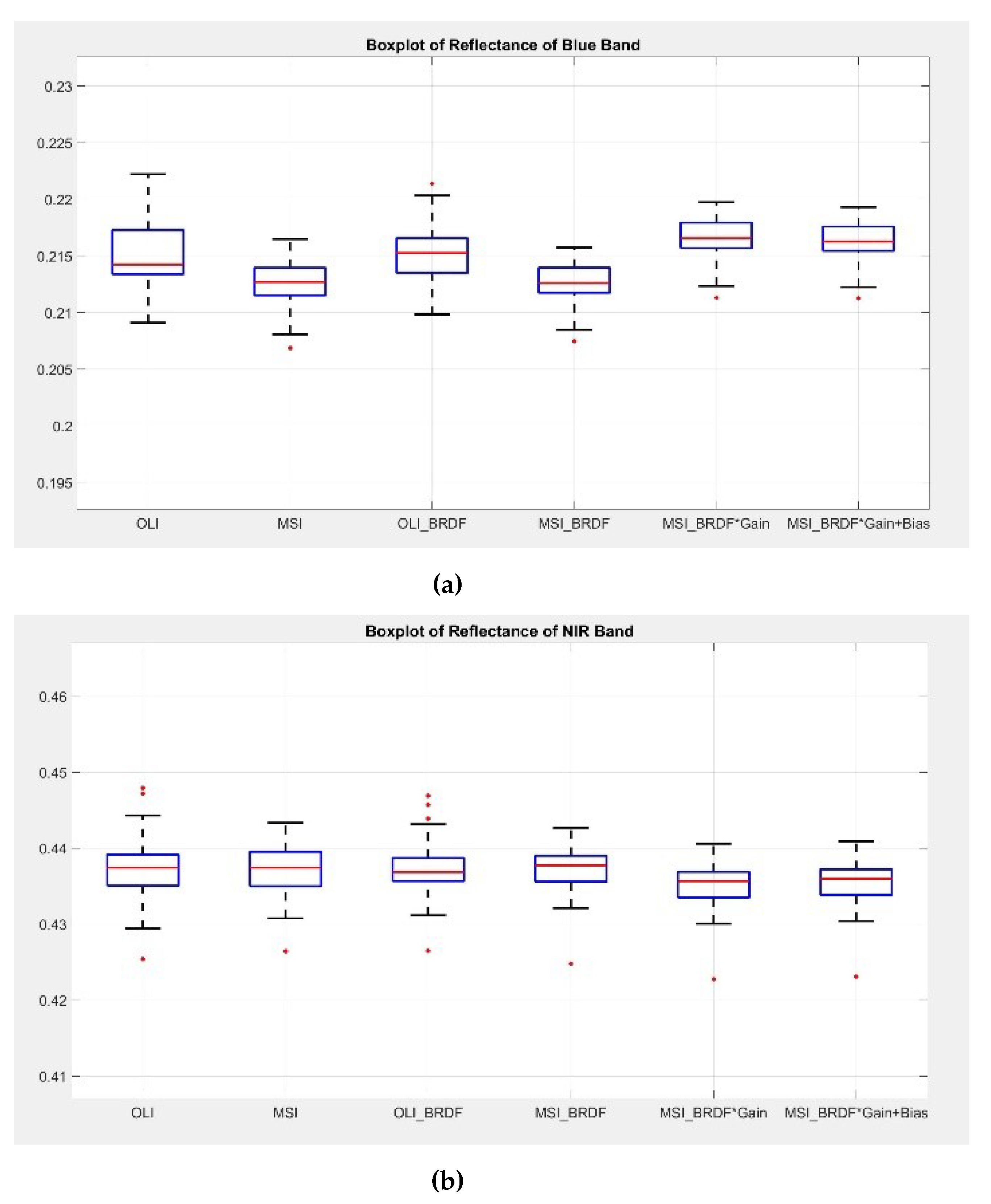
Figure 7a,b shows boxplots of the blue and NIR band TOA reflectances for both sensors, respectively. In each figure, the first two boxplots show the OLI and MSI reflectances after SBAF correction alone. The next two plots show the OLI and MSI reflectances after SBAF and BRDF normalization. The final two plots show the MSI reflectances after application of gain only and application of gain and a nonzero bias, respectively. Boxplots of the observed reflectance distribution were analyzed because the temporal sampling frequency for both sensors was not the same, especially due to exclusion of cloudy scenes; the difference in the resulting number of usable scenes for the analysis would adversely bias the estimated mean reflectances towards a lower uncertainty for the sensor with fewer scenes. The boxplots also suggest the occurrence of band-dependent skewing in the TOA reflectance distributions away from a normal distribution, providing support for selection of a nonparametric validation analysis.
As seen in Figure 7a, the OLI TOA reflectance after BRDF normalization was slightly higher than the corresponding MSI TOA reflectance after SBAF correction and BRDF normalization. After application of either set of gains to the MSI reflectances, the differences were decreased by essentially the same amount. Although the relative difference between the OLI and MSI reflectance distributions was small, application of the cross-calibration gains and offsets observably improved inter-sensor agreement across all bands. Application of either set of cross-calibration gain improved agreement in all bands except the NIR band (Figure 7b). The Wilcoxon rank sum analysis was performed assuming a null hypothesis of zero gain or bias vs. the alternative hypothesis of nonzero gain or bias; the significance level was set to 0.05. The resulting p-values and null hypothesis rejection/failure to reject decisions for the tests in each band are shown in Table 10.
Based on the test results shown in Table 10, the following observations can be made:
- There was insufficient evidence to indicate differences between OLI and MSI mean TOA reflectances in the coastal aerosol, red, and SWIR2 bands when either set of gains was applied. The offsets were not statistically significant, and the gains were essentially equal.
- There was sufficient evidence to indicate differences between OLI and MSI mean TOA reflectances in the NIR band. Using the gain with offset, the difference was less statistically significant, perhaps not surprising given the observed outliers in the OLI reflectances.
- There was sufficient evidence to indicate differences in the green band.
- Both tests found sufficient evidence to indicate differences in TOA reflectance in the blue band when gain with offset was applied. This is likely due to the apparent non-normality observed in the OLI reflectances. The disagreement with the Wilcoxon test results when gain only was considered should be expected, as the cross-calibration offset was found to be significant in this band.
- Both tests found insufficient evidence to indicate differences in reflectance in the SWIR1 band when gain with offset was considered but sufficient evidence to indicate differences when gain only was considered. However, the strength of evidence in the gain-only case was very “weak”, as the p-value was close to 0.05. This may be due to the fact that the variance in MSI reflectance was slightly larger than the corresponding OLI reflectance variance, which would violate the assumption of equal variance required in the two-sample t test.
With the exception of the SWIR1 band, the OLI reflectance variances were larger than the corresponding MSI reflectance variances due to the much larger amount of available OLI data. There is also a noticeable temporal inconsistency in the available MSI reflectance data, which may be accounted for by the various changes to the Sentinel 2A data processing flow creating different baseline versions throughout the lifetime [33]. An additional consideration is that the Algodones Dunes site is not considered an appropriate PICS for sensor calibration due to its more highly variable surface characteristics and weather conditions. However, better calibration results were obtained for this site using the set of cross-calibration gains with offsets in all bands.
Overall, both sets of estimated gains were shown to improve the agreement between sensors for both PICS and sites such as Algodones Dunes in all bands, with the possible exception of the NIR band. Based on this analysis, the full gain + offset calibration model yielded “better” agreement between the MSI and OLI, especially in the blue band given its more significant offset. Table 11 shows the final cross calibration gains and offsets recommended for each MSI band.
4. Conclusions
A new cross-calibration technique was developed for the Sentinel 2A MSI and Landsat 8 OLI sensors with the object of increasing data harmonization between them. The cross calibration was developed using reflectance data from Saharan Desert PICS and dark targets such as Lake Tahoe and the Libyan volcano. Specific uncertainties associated with each step of the proposed cross calibration were estimated, as was the overall uncertainty associated with the entire process. Finally, the proposed cross calibration was validated using image data acquired over the Algodones Dunes site.
For the blue band, the SBAF values for the desert PICS and Libyan volcanic site were within 3% to 4% of unity and within 8% of unity for Lake Tahoe for the blue band. For the other bands, the SBAF values were generally within 1% to 2% of unity.
The proposed 4-angle BRDF normalization model demonstrated good potential for normalization in the longer wavelength bands but less potential for normalization in the coastal aerosol and blue bands. This can be explained by the fact that these bands are more sensitive to changes in atmospheric characteristics than direct changes in solar position. Though the relation of reflectance with respect to SZA and VZA is quadratic to maintain model and correction simplicity, the relationship was assumed to be linear. Not surprisingly, an extended version of the proposed four-angle model accounting for quadratic and interaction terms in SZA and VZA provided additional normalization, particularly in the shorter wavelength bands. Hence, researchers can use this model for a better understanding of the BRDF property of a surface.
When cross-calibration gains and nonzero offsets are considered, the blue and red bands exhibited the largest deviations from unity gain, on the orders of −2.6% and −1.44%, respectively. The coastal aerosol band was found to have the largest regression standard error (0.0326) and lowest corresponding R-square value (approximately 97%) for this parameter. With the exception of the blue band, the offset was not found to be statistically significant. When cross-calibration gains were considered with forced zero offsets, the blue band again exhibited the largest deviation from unity gain, on the order of 1.86%.
Overall, the total uncertainty in the proposed cross calibration is approximately 6.8%. The largest contribution is due to the uncertainty in each sensor’s calibration (on the order of 3% for OLI and of 5% for MSI). The next most significant sources contributing to the overall uncertainty were (i) differences in solar zenith and azimuth angles caused by the difference in local overpass times (on the order of 2.27%); (ii) site nonuniformity (on the order of 1.8%); (iii) differences in the sensor RSR measurement (on the order of 1% for MSI); (iv) potential shifts in spectral filter center wavelength and/or bandwidth (on the order of the 0.82% in the SWIR2 band); and (v) uncertainties in image registration error (on the order of 0.55% across all bands). Uncertainties due to differences in sensor spatial resolution contributed much smaller levels to the overall uncertainty.
Author Contributions
M.M.F. contributed to the conceptualization, methodology, investigation, analysis software development, and writing of the manuscript. M.K. contributed significantly to the conceptualization, methodology, investigation, and subsequent reviews of the article. L.L. provided important suggestions and directions, also helped with the 4 angle multi-linear BRDF model concept. D.H. provided and administered the funding of this research, and provided final review of the manuscript. All authors have read and agreed to the published version of the manuscript.
Funding
This research was funded by USGS grant number G14AC00370.
Acknowledgments
The authors thank Tim Ruggles for providing assistance with proof reading.
Conflicts of Interest
The authors declare no conflict of interest.
References
- Helder, D.L.; Markham, B.L.; Thome, K.J.; Barsi, J.A.; Chander, G.; Malla, R. Updated Radiometric Calibration for the Landsat-5 Thematic Mapper Reflective Bands. IEEE Trans. Geosci. Remote Sens. 2008, 10, 3309–3325. [Google Scholar] [CrossRef]
- Markham, B.L.; Helder, D.L. Forty-year calibrated record of earth-reflected radiance from Landsat: A review. Remote Sens. Environ. 2012, 122, 30–40. [Google Scholar] [CrossRef] [Green Version]
- Helder, D.L.; Basnet, B.; Morstad, D. Optimized identification of worldwide radiometric pseudo-invariant calibration sites. Can. J. Remote Sens. 2010, 36, 527–539. [Google Scholar] [CrossRef]
- Nagaraja Rao, C.R.; Chen, J. Inter-satellite calibration linkages for the visible and near-infared channels of the Advanced Very High Resolution Radiometer on the NOAA-7,-9, and-11 spacecraft. Int. J. Remote Sens. 1995, 16, 1931–1942. [Google Scholar] [CrossRef]
- Cosnefroy, H.; Leroy, M.; Briottet, X. Selection and characterization of Saharan and Arabian desert sites for the calibration of optical satellite sensors. Remote Sens. Environ. 1996, 58, 101–114. [Google Scholar] [CrossRef]
- Chander, G.; Angal, A.; Helder, D.L.; Mishra, N.; Wu, A. Preliminary assessment of several parameters to measure and compare usefulness of the CEOS reference pseudo-invariant calibration sites. Remote Sens. 2010, 7826, 78262L. [Google Scholar]
- Morstad, D.L.; Helder, D.L. Use of Pseudo-Invariant Sites for Long-Term Sensor Calibration. Int. Geosci. Remote Sens. Symp. (IGARSS) 2008, 1, I-253–I-256. [Google Scholar] [CrossRef]
- Hasan, M.N.; Shrestha, M.; Leigh, L.; Helder, D. Evaluation of an Extended PICS (EPICS) for Calibration and Stability Monitoring of Optical Satellite Sensors. Remote Sens. 2019, 11, 1755. [Google Scholar] [CrossRef] [Green Version]
- Shrestha, M.; Leigh, L.; Helder, D. Classification of North Africa for Use as an Extended Pseudo Invariant Calibration Sites (EPICS) for Radiometric Calibration and Stability Monitoring of Optical Satellite Sensors. Remote Sens. 2019, 11, 875. [Google Scholar] [CrossRef] [Green Version]
- Philippe Teillet, M.; Fedosejevs, G.; Thome, K.J. Spectral band difference effects on radiometric cross-calibration between multiple satellite sensors in the Landsat solar-reflective spectral domain. In Sensors, Systems, and Next-Generation Satellites; International Society for Optics and Photonics: Bellingham, WA, USA, 2004. [Google Scholar] [CrossRef]
- Chander, G.; Mishra, N.; Helder, D.; Aaron, D.; Choi, T.; Angal, A.; Xiong, X. Use of EO-1 Hyperion data to calculate spectral band adjustment factors (SBAF) between the L7 ETM+ and Terra MODIS sensors. In Proceedings of the 2010 IEEE International Geoscience and Remote Sensing Symposium, Honolulu, HI, USA, 25–30 July 2010; pp. 1667–1670. [Google Scholar] [CrossRef]
- Chander, G.; Mishra, N.; Helder, D.L.; Aaron, D.B.; Angal, A.; Choi, T.; Xiong, X.; David Doelling, R. Applications of Spectral Band Adjustment Factors(SBAF) for Cross-Calibration. Geosci. Remote Sens. IEEE Trans. 2013, 51, 1267–1281. [Google Scholar] [CrossRef]
- Liu, J.J.; Li, Z.; Qiao, Y.L.; Liu, Y.J.; Zhang, Y.X. A new method for cross-calibration of two satellite sensors. Int. J. Remote Sens. 2004, 25, 5267–5281. [Google Scholar] [CrossRef]
- Roujean, J.L.; Leroy, M.; Deschamps, P.Y. A bi-directional reflectance model of the Earth’s surface for the correction of remote sensing data. J. Geophys. Res. 1992, 97, 20455–20468. [Google Scholar] [CrossRef]
- Schlapfer, D.; Richter, R.; Feingersh, T. Operational BRDF Effects Correction for Wide-Field-of-View Optical Scanners (BREFCOR). IEEE Trans. Geosci. Remote Sens. 2015, 53, 1855–1864. [Google Scholar] [CrossRef] [Green Version]
- Mishra, N.; Helder, D.; Angal, A.; Choi, J.; Xiong, X. Absolute Calibration of Optical Satellite Sensors Using Libya 4 Pseudo Invariant Calibration Site. Remote Sens. 2014, 6, 1327–1346. [Google Scholar] [CrossRef] [Green Version]
- Lacherade, S.; Fougnie, B.; Henry, P.; Gamet, P. Cross Calibration Over Desert Sites: Description, Methodology, and Operational Implementation. IEEE Trans. Geosci. Remote Sens. 2013, 51, 1098–1113. [Google Scholar] [CrossRef]
- Mishra, N.; Haque, M.O.; Leigh, L.; Aaron, D.; Helder, D.; Markham, B. Radiometric Cross Calibration of Landsat 8 Operational Land Imager (OLI) and Landsat 7 Enhanced Thematic Mapper Plus (ETM+). Remote Sens. 2014, 6, 12619–12638. [Google Scholar] [CrossRef] [Green Version]
- Li, S.; Ganguly, S.; Dungan, J.L.; Wang, W.L.; Nemani, R.R. Sentinel-2 MSI Radiometric Characterization and Cross-Calibration with Landsat-8 OLI. Adv. Remote Sens. 2017, 6, 147–159. [Google Scholar] [CrossRef] [Green Version]
- Pinto, C.T.; Ponzoni, F.J.; Castro, R.M.; Leigh, L.; Kaewmanee, M.; Aaron, D.; Helder, D. Evaluation of the uncertainty in the spectral band adjustment factor (SBAF) for cross-calibration using Monte Carlo simulation. Remote Sens. Lett. 2016, 7, 837–846. [Google Scholar] [CrossRef]
- Chander, G.; Helder, D.L.; Aaron, D.; Mishra, N.; Shrestha, A.K. Assessment of Spectral, Misregistration, and Spatial Uncertainties Inherent in the Cross-Calibration Study. IEEE Trans. Geosci. Remote Sens. 2013, 51, 1282–1296. [Google Scholar] [CrossRef]
- Gorroño, J.; Banks, A.C.; Fox, N.P.; Underwood, C. Radiometric inter-sensor cross-calibration uncertainty using a traceable high accuracy reference hyperspectral imager. ISPRS J. Photogramm. Remote Sens. 2013, 130, 393–417. [Google Scholar] [CrossRef] [Green Version]
- The Worldwide Reference System. Available online: https://landsat.gsfc.nasa.gov/the-worldwide-reference-system (accessed on 8 November 2017).
- Gascon, F.; Bouzinac, C.; Thépaut, O.; Jung, M.; Francesconi, B.; Louis, J.; Lonjou, V.; Lafrance, B.; Massera, S.; Gaudel-Vacaresse, A.; et al. Copernicus Sentinel-2A Calibration and Products Validation Status. Remote Sens. 2017, 9, 584. [Google Scholar] [CrossRef] [Green Version]
- Sentinel 2 Handbook. Available online: https://sentinel.esa.int/documents/247904/685211/Sentinel-2/User/Handbook (accessed on 8 November 2017).
- Sentinel 2 Technical guide. Available online: https://earth.esa.int/web/technical-guides/sentinel-2-msi/performance (accessed on 8 November 2017).
- Barsi, J.A.; Lee, K.; Kvaran, G.; Markham, B.L.; Jeffrey Pedelty, A. The Spectral Response of the Landsat-8 Operational Land Imager. Remote Sens. 2014, 6, 10232–10251. [Google Scholar] [CrossRef] [Green Version]
- Harika, V. Normalization of Pseudo-invariant Calibration Sites for Increasing the Temporal Resolution and Long-Term Trending. Master’s Thesis, South Dakota State University, Brookings, SD, USA, 2017. Available online: https://openprairie.sdstate.edu/etd/2180/ (accessed on 21 September 2018).
- Farhad, M.M. Cross Calibration and Validation of Landsat 8 OLI and Sentinel 2A MSI. Master’s Thesis, Department of Electrical Engineering, South Dakota State University, Brookings, SD, USA, 2018. [Google Scholar]
- Sentinel 2 Data Quality Reports. 8 February 2018. Available online: https://sentinel.esa.int/documents/247904/685211/Sentinel-2-Data-Quality-Report (accessed on 28 February 2018).
- Brian Markham. Available online: https://landsat.usgs.gov/sites/default/files/documents/landsat_science_team/2018-02_Day1_Markham_Landsat%20Calibration%20and%20Validation.pdf (accessed on 21 September 2018).
- Sentinel 2 Technical guide and performance. Available online: https://earth.esa.int/web/sentinel/technical-guides/sentinel-2-msi/performance (accessed on 21 September 2018).
- Sentinel2 processing baselines. Available online: https://sentinel.esa.int/web/sentinel/missions/sentinel-2/news/-/article/new-processing-baseline-02-04-for-sentinel-2a-products (accessed on 7 March 2018).
Figure 1.
Relative spectral response of Operational Land Imager (OLI; solid line) and Multispectral Instrument (MSI; dotted line). (a) shows the RSR comparison for VNIR bands and (b) shows the RSR comparison for SWIR bands.
Figure 1.
Relative spectral response of Operational Land Imager (OLI; solid line) and Multispectral Instrument (MSI; dotted line). (a) shows the RSR comparison for VNIR bands and (b) shows the RSR comparison for SWIR bands.

Figure 2.
Location of the bright and dark targets. (a) shows the location of 6 bright targets recommended by CNES, (b1) shows the volcanic site and (b2) shows a Landsat True Color Image of Lake Tahoe.
Figure 2.
Location of the bright and dark targets. (a) shows the location of 6 bright targets recommended by CNES, (b1) shows the volcanic site and (b2) shows a Landsat True Color Image of Lake Tahoe.

Figure 3.
Hyperion spectral profiles for Libya 4: (a) before ±2.5σ filter application and (b) after filter application.
Figure 3.
Hyperion spectral profiles for Libya 4: (a) before ±2.5σ filter application and (b) after filter application.

Figure 4.
TOA reflectance vs. spherical coordinate solar angles for NIR band before and after angular conversion.
Figure 4.
TOA reflectance vs. spherical coordinate solar angles for NIR band before and after angular conversion.

Figure 5.
Before and after Bidirectional Reflectance Distribution Function (BRDF)-normalized TOA eeflectance of OLI over the Sudan1 site for the CA and SWIR1 bands with the proposed multi-linear 4-angle BRDF model.
Figure 5.
Before and after Bidirectional Reflectance Distribution Function (BRDF)-normalized TOA eeflectance of OLI over the Sudan1 site for the CA and SWIR1 bands with the proposed multi-linear 4-angle BRDF model.

Figure 6.
Regression line for the cross calibration of OLI and MSI.

Figure 7.
Boxplots of OLI and MSI TOA before and after BRDF normalization and of MSI TOA after applying both sets of gain in the Algodones Dunes: (a) blue band and (b) NIR band.
Figure 7.
Boxplots of OLI and MSI TOA before and after BRDF normalization and of MSI TOA after applying both sets of gain in the Algodones Dunes: (a) blue band and (b) NIR band.


Table 1.
Target sites locations and ROI used.
| Target Site | WRS2 Path | WRS2 Row | Center Lattitude | Center Longitude | Site Length | Site Width |
|---|---|---|---|---|---|---|
| Libya1 | 187 | 43 | 24.71 | 13.49 | 33,990 m | 34,920 m |
| Libya4 | 181 | 40 | 28.55 | 23.38 | 21,690 m | 19,980 m |
| Niger2 | 188 | 45 | 21.36 | 10.55 | 25,320 m | 33,480 m |
| Sudan1 | 177 | 45 | 21.58 | 27.70 | 38,400 m | 22,680 m |
| Lake Tahoe | 43 | 33 | 39.09 | −120.03 | 11,220 m | 11,190 m |
| Volcanic Near Libya | 184 | 43 | 24.86 | 23.77 | 5962 m | 9118 m |
Table 2.
Libya 4 Spectral Band Adjustment Factor (SBAF) and standard deviation by band.
| Band | CA | Blue | Green | Red | NIR | SWIR1 | SWIR2 |
|---|---|---|---|---|---|---|---|
| SBAF | 1.0015 | 0.9594 | 1.0066 | 0.9790 | 0.9996 | 0.9988 | 0.9989 |
| Standard Daviation | 0.0001 | 0.0027 | 0.0013 | 0.0010 | 0.0050 | 0.0030 | 0.0070 |
Table 3.
Target-site SBAFs by band.
| Site | Hyperion Scenes Used | Bands | ||||||
|---|---|---|---|---|---|---|---|---|
| CA | Blue | Green | Red | NIR | SWIR1 | SWIR2 | ||
| Libya 1 | 81 | 1.0017 | 0.9603 | 1.0217 | 0.9777 | 0.9990 | 0.9988 | 1.0010 |
| Niger 2 | 12 | 1.0016 | 0.9681 | 1.0112 | 0.9794 | 1.0003 | 0.9989 | 1.0002 |
| Sudan 1 | 152 | 1.0015 | 0.9643 | 1.0131 | 0.9793 | 1.0001 | 0.9991 | 1.0003 |
| Lake Tahoe | 25 | 1.0201 | 1.0801 | 0.9820 | 1.0180 | 1.0050 | 0.9980 | 0.9980 |
| Volcanic near Libya | 4 | 1.0015 | 0.9659 | 1.0058 | 0.9800 | 1.0001 | 0.9990 | 0.9981 |
Table 4.
Percentage temporal uncertainty in OLI TOA reflectance of Libya4 Pseudo-Invariant Calibration Site (PICS) data before and after BRDF normalization.
Table 4.
Percentage temporal uncertainty in OLI TOA reflectance of Libya4 Pseudo-Invariant Calibration Site (PICS) data before and after BRDF normalization.
| Bands | Before Correction | Normalization with Linear SZA based Model (Spherical Coordinate) | Normalization with Quadratic SZA based Model (Spherical Coordinate) | Normalization with Multi-linear 4 Angle BRDF Model (Plane Cartesian Coordinate) | Normalization with Quadratic Multi-linear 4-angle BRDF Model with Interactions (Plane Cartesian Coordinate) |
|---|---|---|---|---|---|
| CA | 1.5 | 1.19 | 1.08 | 1.19 | 0.98 |
| Blue | 1.25 | 1.19 | 1.12 | 1.15 | 0.85 |
| Green | 1.08 | 0.93 | 0.93 | 0.89 | 0.78 |
| Red | 1.23 | 0.85 | 0.84 | 0.81 | 0.74 |
| NIR | 1.28 | 0.73 | 0.69 | 0.65 | 0.65 |
| SWIR1 | 2.08 | 0.61 | 0.60 | 0.58 | 0.53 |
| SWIR2 | 2.48 | 1.91 | 1.80 | 1.76 | 1.52 |
Table 5.
Scene pairs used for cross calibration.
| Site | WRS2 Path/Row | Number of Scene Pairs | Coincident/Near Coincident |
|---|---|---|---|
| Libya 1 | 187/043 | 4 | Coincident |
| Libya 4 | 181/040 | 8 | Coincident |
| Niger 2 | 188/045 | 7 | Coincident |
| Sudan 1 | 177/045 | 9 | Coincident |
| Lake Tahoe | 043/033 | 2 | Coincident |
| Libya Volcano | 184/043 | 5 | Near Coincident |
Table 6.
Cross-calibration gain statistics with nonzero offset.
| Bands | Coefficient | Estimate | Standard Error | t-Stat | p-Value | Null Hypothesis |
|---|---|---|---|---|---|---|
| CA | Bias | 0.0002 | 0.0065 | 0.024 | 0.981 | Failed to Reject |
| Gain | 1.0012 | 0.0326 | 30.668 | Reject | ||
| Blue | Bias | 0.0092 | 0.0035 | 2.605 | 0.0145 | Reject |
| Gain | 0.9741 | 0.0176 | 55.384 | Reject | ||
| Green | Bias | 0.0011 | 0.0020 | 0.509 | 0.6147 | Fail to Reject |
| Gain | 1.0046 | 0.0075 | 133.598 | Reject | ||
| Red | Bias | 0.0031 | 0.0019 | 1.621 | 0.1161 | Fail to Reject |
| Gain | 0.9856 | 0.0048 | 206.628 | Reject | ||
| NIR | Bias | 0.0016 | 0.0015 | 1.031 | 0.311 | Fail to Reject |
| Gain | 0.9923 | 0.0031 | 315.917 | Reject | ||
| SWIR1 | Bias | 0.0018 | 0.0019 | 0.962 | 0.3442 | Fail to Reject |
| Gain | 0.9922 | 0.0031 | 315.498 | Reject | ||
| SWIR 2 | Bias | 0.0011 | 0.0017 | 0.635 | 0.5301 | Fail to Reject |
| Gain | 1.0051 | 0.0034 | 297.390 | Reject |
Table 7.
Cross-calibration gain statistics with forced 0 offset.
| Bands | Estimate of Gain | SE | t-Stat | p-Value | Null Hypothesis |
|---|---|---|---|---|---|
| CA | 1.0020 | 0.0052 | 193.63 | Reject | |
| Blue | 1.0186 | 0.0044 | 231.05 | Reject | |
| Green | 1.0083 | 0.0024 | 415.29 | Reject | |
| Red | 0.9928 | 0.0019 | 528.78 | Reject | |
| NIR | 0.9952 | 0.0013 | 770.69 | Reject | |
| SWIR1 | 0.9949 | 0.0013 | 741.21 | Reject | |
| SWIR2 | 1.0070 | 0.0014 | 711.25 | Reject |
Table 8.
Uncertainty due to site nonuniformity.
| Band | Libya4 | Libya1 | Niger2 | Sudan1 |
|---|---|---|---|---|
| CA | 1.56 | 1.77 | 0.86 | 0.96 |
| Blue | 1.35 | 1.75 | 1.13 | 1.23 |
| Green | 1.80 | 1.79 | 1.30 | 1.22 |
| Red | 1.36 | 1.25 | 1.43 | 1.29 |
| NIR | 1.54 | 1.26 | 1.39 | 1.26 |
| SWIR1 | 1.35 | 1.26 | 0.95 | 0.88 |
| SWIR2 | 1.32 | 1.07 | 1.07 | 1.01 |
Table 9.
Summary of all the uncertainties.
| Domain | Source of Uncertainty | Uncertainty (%) |
|---|---|---|
| Spectral | Measured RSR | 1.000 |
| Spectral Filter shift | 0.820 | |
| Spectral Bandwidth Change | 0.280 | |
| Spatial | Registration Error | 0.026 |
| Spatial resolution Mismatch | 0.002 | |
| Site | 1.800 | |
| Temporal | Overpass Time Difference | 2.270 |
| Atmospheric Variation | 1.290 | |
| Sensor | MSI Calibration | 5.000 |
| OLI Calibration | 3.000 | |
| Total Uncertainty | 6.768 | |
Table 10.
Wilcoxon rank sum test results for cross calibration gain applied to MSI reflectances.
| Bands | Set of Gain | Wilcoxon Rank Sum Test | |
|---|---|---|---|
| Null Hypothesis | p-Value | ||
| CA | Gain | Failed to Reject | 0.2846 |
| Gain and Bias | Failed to Reject | 0.2529 | |
| Blue | Gain | Reject | 0.0030 |
| Gain and Bias | Failed to Reject | 0.1410 | |
| Green | Gain | Failed to Reject | 0.0933 |
| Gain and Bias | Failed to Reject | 0.1007 | |
| Red | Gain | Failed to Reject | 0.4076 |
| Gain and Bias | Failed to Reject | 0.8719 | |
| NIR | Gain | Reject | 0.0015 |
| Gain and Bias | Reject | 0.0080 | |
| SWIR1 | Gain | Reject | 0.0312 |
| Gain and Bias | Failed to Reject | 0.1007 | |
| SWIR2 | Gain | Failed to Reject | 0.0877 |
| Gain and Bias | Failed to Reject | 0.1069 | |
Table 11.
Recommended cross calibration gain and bias.
| Bands | CA | Blue | Green | Red | NIR | SWIR1 | SWIR2 |
|---|---|---|---|---|---|---|---|
| Gain | 1.0012 | 0.9740 | 1.0046 | 0.9856 | 0.9923 | 0.9922 | 1.0051 |
| Offset | 0.0002 | 0.0092 | 0.0010 | 0.0030 | 0.0016 | 0.0018 | 0.0011 |
© 2020 by the authors. Licensee MDPI, Basel, Switzerland. This article is an open access article distributed under the terms and conditions of the Creative Commons Attribution (CC BY) license (http://creativecommons.org/licenses/by/4.0/).
Share and Cite
MDPI and ACS Style
Farhad, M.M.; Kaewmanee, M.; Leigh, L.; Helder, D. Radiometric Cross Calibration and Validation Using 4 Angle BRDF Model between Landsat 8 and Sentinel 2A. Remote Sens. 2020, 12, 806. https://0-doi-org.brum.beds.ac.uk/10.3390/rs12050806
AMA Style
Farhad MM, Kaewmanee M, Leigh L, Helder D. Radiometric Cross Calibration and Validation Using 4 Angle BRDF Model between Landsat 8 and Sentinel 2A. Remote Sensing. 2020; 12(5):806. https://0-doi-org.brum.beds.ac.uk/10.3390/rs12050806
Chicago/Turabian StyleFarhad, M M, Morakot Kaewmanee, Larry Leigh, and Dennis Helder. 2020. "Radiometric Cross Calibration and Validation Using 4 Angle BRDF Model between Landsat 8 and Sentinel 2A" Remote Sensing 12, no. 5: 806. https://0-doi-org.brum.beds.ac.uk/10.3390/rs12050806
Note that from the first issue of 2016, this journal uses article numbers instead of page numbers. See further details here.