Coherence-Factor-Based Rough Surface Clutter Suppression for Forward-Looking GPR Imaging

Abstract

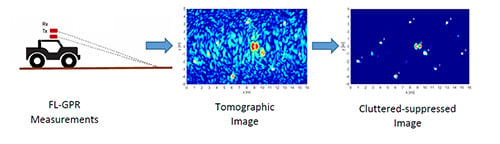
We present an enhanced imaging procedure for suppression of the rough surface clutter arising in forward-looking ground-penetrating radar (FL-GPR) applications. The procedure is based on a matched filtering formulation of microwave tomographic imaging, and employs coherence factor (CF) for clutter suppression. After tomographic reconstruction, the CF is first applied to generate a “coherence map” of the region in front of the FL-GPR system illuminated by the transmitting antennas. A pixel-by-pixel multiplication of the tomographic image with the coherence map is then performed to generate the clutter-suppressed image. The effectiveness of the CF approach is demonstrated both qualitatively and quantitatively using electromagnetic modeled data of metallic and plastic shallow-buried targets.

1. Introduction

Microwave imaging has undergone significant advances in the last two decades, owing to its increased adoption and broad application in a variety of disciplines, including applied geophysics, planetary exploration, and emerging radar technologies [1,2,3,4,5,6,7]. Forward-looking ground penetrating radar (FL-GPR) is one such technology that employs microwave imaging for detection of targets buried at shallow depths in the ground. Unlike its ground-coupled or near-ground down-looking ground penetrating radar (DL-GPR) counterparts, FL-GPR provides standoff sensing capability, which allows fast scanning of large areas for real-time target detection. This capability, however, comes at the expense of energy backscattered from the illuminated targets and limited image spatial resolution [8,9,10,11,12,13,14,15]. Further, the rough ground surface generates clutter that tends to obscure the buried targets, rendering target detection difficult and challenging [12,13,14].

Rough surface clutter suppression for array-based FL-GPR imaging was addressed in [11,14,16,17,18,19,20,21,22,23,24]. In [16], an ambiguity function based detector was proposed which exploits time-frequency characterization of target and clutter scattering for performance enhancement. Frequency subband processing was exploited in [11] to obtain the best contrast between target and clutter signals, whereas recursive side-lobe minimization algorithm for reconstructing FL-GPR images with reduced clutter was proposed in [17]. Coherent integration of measurements corresponding to multiple radar platform positions was demonstrated in [18] for rough surface clutter suppression, whereas a nonlinear combining approach that exploits a similarity measure was developed in [19] to adaptively mitigate imaging artifacts. In [20], localized clutter outside of the region of interest was suppressed prior to sparse reconstruction. A real-time three-dimensional (3-D) model of the rough surface scattering was proposed in [21], which can be subtracted from the FL-GPR measurements to reduce the clutter. A multi-view approach based on the likelihood ratio tests (LRT) detector was proposed in [14] and its adaptive counterpart was presented in [22] for effective detection of low-signature targets in the presence of rough surface clutter. A robust LRT was designed in [23] based on the least favorable target and clutter densities to maximize the worst-case detection performance over all feasible target and clutter models in FL-GPR images. In [24], infrared imagery was used to eliminate false alarms in FL-GPR.

On the other hand, a variety of image formation approaches have been considered in the context of array-based FL-GPR imaging. The most commonly used algorithms are back-projection, frequency-wavenumber migration, and scalar inverse scattering [12,25,26]. These algorithms rely on a scalar representation of the electromagnetic field, for which the relevant Green’s function is simplified by assuming a free-space propagation model. Within the framework of linear inverse scattering, a two-dimensional imaging algorithm for bistatic FL-GPR systems was recently proposed in [15], whereas an inverse processing scheme that exploits the intrinsic multi-aperture nature of the FL-GPR geometry was designed in [14]. Data-adaptive approaches for FL-GPR have also been proposed in the literature [10,13]. Amplitude and phase estimation and rank-deficient robust Capon beamforming were presented in [10], while an iterative hyperparameter-free maximum a posteriori probability algorithm was proposed in [13].

In this paper, we present an FL-GPR image enhancement procedure that employs tomographic imaging and coherence-factor (CF) based masking operation for rough surface clutter suppression. More specifically, we first employ a matched-filtering (MF) based tomographic imaging approach for image formation, which exploits the vectorial nature of the incident and scattered electric fields, in conjunction with coherent combining of multiple measurements from different aperture positions. This approach builds on the MF formulation of [27] for DL-GPR imaging. Following image reconstruction, we perform a masking operation with a coherence map of the scene for clutter suppression. The coherence map is generated using the CF, which represents a measure of the relative coherence of the received signals across all antennas. We consider three variants of the CF, namely, the amplitude CF (ACF), the phase CF (PCF), and the sign CF (SCF) [28,29,30]. The capability of the proposed procedure to significantly suppress the clutter generated by the backscattering from a rough surface is demonstrated using near-field electromagnetic modeled numerical data corresponding to a scene with both plastic and metallic targets buried at shallow depths below a rough interface [31]. The improvements achievable are quantified in terms of the image-domain signal-to-clutter ratio (SCR), starting with the preliminary investigation reported in [32]. We show that all variants of the CF successfully suppress the rough surface clutter with comparable SCR values, and the hybrid MF-based imaging and CF-based masking procedure outperforms the case when CF masking is used in conjunction with standard back-projection (BP). It is noted that two-dimensional (2D) versions of the CF, recently proposed in [33] for sidelobe suppression in radar imaging, can also be employed in the proposed scheme. However, as our objective is to demonstrate the offerings of the hybrid procedure and not specifically identify an optimal method for coherence map generation, we will not consider the 2D versions in this paper.

The remainder of this paper is organized as follows. The various methods considered in this paper are presented in Section 2. More specifically, the MF-based tomographic imaging algorithm is described in Section 2.1, while the BP algorithm is briefly discussed in Section 2.2. The CF-based image enhancement method is presented in Section 2.3, wherein the three variants of CF and the SCR in the image domain are defined. In Section 3, we describe the considered FL-GPR configuration and simulation set up, and provide both the imaging and CF-based enhanced results. BP-based results are also presented for comparison therein. Insights into the performance of the proposed scheme are provided in Section 4. Conclusion follows in Section 5.

2. Methods

2.1. Matched-Filtering-Based Near-Field Tomographic Imaging

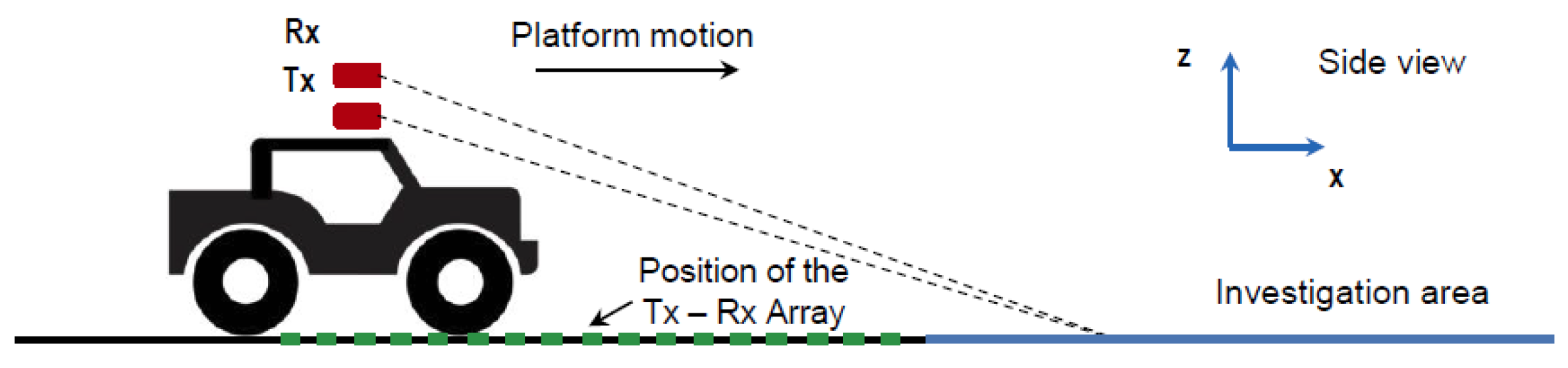
We consider an FL-GPR system consisting of an $N_T$-element linear transmit array and an $N_R$-element linear receive array. The transmit and receive antennas are oriented parallel to the y-axis in the $yz$-plane and mounted on top of a vehicle at different heights (z-coordinates). The investigation domain is located on the ground in front of the vehicle along the x-axis (see Figure 1). The transmitters are assumed to be activated sequentially, with simultaneous reception at all receivers, as the vehicle moves forward. For convenience, we assume that a single transmitter is active for each platform position. Thus, a full-aperture measurement set comprises $N_T{N}_R$ observations from $N_T$ consecutive platform positions. The frequency band of operation extends from ${\omega }_L$ to ${\omega }_H$.

Considering a 3-D version of the well-known scattering equation, a linear scattering model can be established under the Born approximation for the near-field imaging conditions of the considered scenario as [34].

$${\mathbf{E}}_s({\mathbf{r}}_{rn},{\mathbf{r}}_{tm},\omega )=k_b^2{\int \int }_D\underline{\mathbf{G}}(\mathbf{r},{\mathbf{r}}_{rn},\omega )·{\mathbf{E}}_{\mathrm{inc}}(\mathbf{r},{\mathbf{r}}_{tm},\omega )O\left(\mathbf{r}\right)d\mathbf{r}.$$

(1)

This model represents the relationship between the scattered field ${\mathbf{E}}_s$ from the investigation domain D, recorded at the n-th receive location ${\mathbf{r}}_{rn}$ with the m-th active transmitter at ${\mathbf{r}}_{tm}$, and the unknown scene reflectivity $O\left(\mathbf{r}\right)$ for angular frequency $\omega$. In (1), $\underline{\mathbf{G}}$ is the dyadic Green’s function of the problem, ${\mathbf{E}}_{\mathrm{inc}}$ is the incident field, which under the Born approximation represents the total field inside the domain D, $k_0=\omega \sqrt{\left({\epsilon }_0{\mu }_0\right)}$ is the free-space wavenumber, $k_b=\sqrt{{\epsilon }_r}{k}_0$ is the wavenumber of the subsurface medium, and $\mathbf{r}$ represents a generic point in the domain D. The vectors $\mathbf{r},{\mathbf{r}}_{tm}$, and ${\mathbf{r}}_{rn}$ are defined as

$$\begin{array}{cc}\hfill {\mathbf{r}}_{tm}& =x_{tm}{\mathbf{x}}_0+y_{tm}{\mathbf{y}}_0+z_{tm}{\mathbf{z}}_0\hfill \\ \hfill {\mathbf{r}}_{rn}& =x_{rn}{\mathbf{x}}_0+y_{rn}{\mathbf{y}}_0+z_{rn}{\mathbf{z}}_0\hfill \\ \hfill \mathbf{r}& =x{\mathbf{x}}_0+y{\mathbf{y}}_0+z{\mathbf{z}}_0,\hfill \end{array}$$

(2)

with ${\mathbf{x}}_0$, ${\mathbf{y}}_0$, and ${\mathbf{z}}_0$ denoting the unit vectors along the x, y, and z directions, respectively. The operator $(·)$ in (1) represents the dyadic product and is implemented as the typical matrix-vector product between the $3\times 3$ matrix Green’s function $\underline{\mathbf{G}}$ and the $3\times 1$ vector incident field ${\mathbf{E}}_{\mathrm{inc}}$. Equation (1) accounts for the dyadic nature of the interaction between the electric field and the probed scene.

Modeling the transmitting elements as Hertzian electric dipoles oriented along ${\mathbf{z}}_0$, the incident electric field can be expressed as

$${\mathbf{E}}_{\mathrm{inc}}(\mathbf{r},{\mathbf{r}}_{tm},\omega )=-j\omega {\mu }_0{I}_{0}l\underline{\mathbf{G}}(\mathbf{r},{\mathbf{r}}_{tm},\omega )·{\mathbf{z}}_{\mathbf{0}},$$

(3)

where $I_{0}l$ is the current moment associated with the short dipole directed along ${\mathbf{z}}_0$ and is assumed to be equal to 1 A·m. Therefore, (1) can be rewritten as

$${\mathbf{E}}_{\mathrm{s}}({\mathbf{r}}_{rn},{\mathbf{r}}_{tm},\omega )=-j\omega {\mu }_0{k}_b^2{\int \int }_D\underline{\mathbf{G}}(\mathbf{r};{\mathbf{r}}_{rn},\omega )·[\underline{\mathbf{G}}(\mathbf{r};{\mathbf{r}}_{tm},\omega )·{\mathbf{z}}_{\mathbf{0}}]O\left(\mathbf{r}\right)d\mathbf{r}.$$

(4)

Under the assumptions that (i) the separation in height between the transmit and receive elements is negligible, and (ii) the targets are either on the ground surface or buried at shallow depths, the dyadic Green’s function and, subsequently, the incident field can be approximated as those modeling propagation in a homogeneous medium having the electromagnetic properties of free-space [34]. That is,

$$\underline{\mathbf{G}}(\mathbf{r},{\mathbf{r}}_s,\omega )=\left[\underline{\mathbf{I}}+\frac{\nabla \nabla }{k_0^2}\right]\frac{e^{-j{k}_0|\mathbf{r}-{\mathbf{r}}_s|}}{4\pi |\mathbf{r}-{\mathbf{r}}_s|},$$

(5)

where $\underline{\mathbf{I}}$ is the unit dyad and $s=rn$ or $tm$.

Dividing the domain D into a finite number of pixels, say Q, we assume only one point scatterer exists per pixel. Ignoring the mutual interactions between scatterers, the point target at the q-th pixel can be modeled as an impulse located at the considered pixel, whose position vector is denoted by ${\mathbf{r}}_{\mathrm{q}}$. As a result, the scattered field from the q-th image pixel recorded by the n-th receiver with the m-th transmitter active and directed along ${\mathbf{z}}_0$ is given by

$${\mathbf{E}}_{\mathrm{s}}({\mathbf{r}}_{rn},{\mathbf{r}}_{tm},\omega )=-j\omega {\mu }_0{k}_0^2\left[\underline{\mathbf{G}}({\mathbf{r}}_{\mathrm{q}},{\mathbf{r}}_{rn},\omega )\right]·[\underline{\mathbf{G}}({\mathbf{r}}_{\mathrm{q}};{\mathbf{r}}_{tm},\omega )·{\mathbf{z}}_0]O\left({\mathbf{r}}_q\right).$$

(6)

If only the z-component of the electric field is measured by the receiving antenna (i.e., through a linear polarized receiving antenna modeled as a short dipole oriented along ${\mathbf{z}}_0$), we can express the recorded electric field $E_{s_z}$ as

$$E_{s_z}({\mathbf{r}}_{rn},{\mathbf{r}}_{tm},\omega )={\mathbf{z}}_0·{\mathbf{E}}_{\mathrm{s}}({\mathbf{r}}_{rn},{\mathbf{r}}_{tm},\omega )=-j\omega {\mu }_0{k}_0^2\left(G_{zx}{G}_{xz}+G_{zy}{G}_{yz}+G_{zz}{G}_{zz}\right)O\left({\mathbf{r}}_q\right),$$

(7)

where the Green’s functions components, $G_{ij}$, with i and j representing the Cartesian coordinates $x,y,z$, can be derived from (5) [5].

With both transmitting and receiving antennas linearly polarized along the z-axis, we define the frequency response $H_{zz}({\mathbf{r}}_{rn},{\mathbf{r}}_{tm},{\mathbf{r}}_{\mathrm{q}},\omega )$ of a filter matched to a point scatterer with unit reflectivity at pixel ${\mathbf{r}}_{\mathrm{q}}$, when the m-th antenna is transmitting and the n-th antenna is receiving, using (7) as

$$H_{zz}({\mathbf{r}}_{rn},{\mathbf{r}}_{tm},{\mathbf{r}}_{\mathrm{q}},\omega )={\left\{-j\omega {\mu }_0{k}_0^2\left(G_{zx}{G}_{xz}+G_{zy}{G}_{yz}+G_{zz}{G}_{zz}\right)\right\}}^{*},$$

(8)

with ‘*’ denoting complex conjugation. The reflectivity estimate ${\widehat{O}}_{nm}\left({\mathbf{r}}_{\mathrm{q}}\right)$ of the q-th pixel is obtained by applying the matched filter to the recorded measurements by the n-th receiver when the m-th antenna is transmitting over the bandwidth of interest as

$${\widehat{O}}_{nm}\left({\mathbf{r}}_{\mathrm{q}}\right)={\int }_{{\omega }_L}^{{\omega }_H}{H}_{zz}({\mathbf{r}}_{\mathrm{q}},{\mathbf{r}}_{tm},{\mathbf{r}}_{rn},\omega )E_{sz}({\mathbf{r}}_{rn},{\mathbf{r}}_{tm},\omega )d\omega .$$

(9)

Note that (9) provides the reflectivity estimate for each pixel as a function of the transmitter and receiver locations. The reflectivity estimate for the pixel at ${\mathbf{r}}_{\mathrm{q}}$, corresponding to all $N_T$ transmitting and $N_R$ receiving z-polarized antennas, can be obtained by exploiting (8) and (9) as,

$$\begin{array}{cc}\hfill \widehat{O}\left({\mathbf{r}}_{\mathrm{q}}\right)& =\sum _{n=1}^{N_{\mathrm{R}}}\sum _{m=1}^{N_{\mathrm{T}}}{\widehat{O}}_{nm}\left({\mathbf{r}}_{\mathrm{q}}\right)\hfill \\ & =j\omega {\mu }_0{k}_0^2\sum _{n=1}^{N_{\mathrm{R}}}\sum _{m=1}^{N_{\mathrm{T}}}{\int }_{{\omega }_L}^{{\omega }_H}{\left(G_{zx}{G}_{xz}+G_{zy}{G}_{yz}+G_{zz}{G}_{zz}\right)}^{*}{E}_{s_z}({\mathbf{r}}_{rn},{\mathbf{r}}_{tm},\omega )d\omega .\hfill \end{array}$$

(10)

The spatial map, $\widehat{O}\left({\mathbf{r}}_{\mathrm{q}}\right)$ of the scene reflectivity is the desired image of the investigated domain D and is the final outcome of the MF-based imaging algorithm. It is noted that coherent integration of measurements corresponding to multiple full apertures, resulting from radar platform motion, can also be employed within the MF imaging framework to reduce artifacts and rough surface clutter prior to the CF-based masking operation [14,18].

2.2. Back-Projection Algorithm

An alternative approach to generating FL-GPR images is the BP algorithm, which is based on scalar wave theory [1]. The mathematical formulation for the BP-based image formation method can be essentially derived by simplifying the dyadic Green’s function in (5) to a scalar model. Thus, the reflectivity estimate at pixel location ${\mathbf{r}}_{\mathrm{q}}$, assuming a free-space propagation model, is achieved as

$${\widehat{O}}^{BP}\left({\mathbf{r}}_{\mathrm{q}}\right)=\sum _{n=1}^{N_{\mathrm{R}}}\sum _{m=1}^{N_{\mathrm{T}}}{\widehat{O}}_{nm}^{BP}\left({\mathbf{r}}_{\mathrm{q}}\right)=\sum _{n=1}^{N_{\mathrm{R}}}\sum _{m=1}^{N_{\mathrm{T}}}{\int }_{{\omega }_L}^{{\omega }_H}{e}^{j{k}_0\left|{\mathbf{r}}_{\mathrm{q}}-{\mathbf{r}}_{tm}\right|}{e}^{j{k}_0\left|{\mathbf{r}}_q-{\mathbf{r}}_{rn}\right|}{E}_{s_z}({\mathbf{r}}_{rn},{\mathbf{r}}_{tm},\omega )d\omega .$$

(11)

The spatial map, ${\widehat{O}}^{BP}\left({\mathbf{r}}_{\mathrm{q}}\right)$, of the scene reflectivity represents the BP-based image of the investigated domain D.

2.3. Coherence-Factor-Based Image Enhancement

In this section, we present the CF-based processing for the enhancement of cluttered FL-GPR images. We consider the following three variants of the CF: the amplitude CF (ACF), the phase CF (PCF), and the sign CF (SCF).

The ACF is defined as the ratio of the total coherent power received by the antenna array (generated by the presence of targets in the domain under investigation) to the total incoherent power (produced by the rough surface clutter for the case under consideration). Mathematically, it can be expressed as [32]

$$\mathrm{ACF}\left({\mathbf{r}}_{\mathrm{q}}\right)=\frac{{\left|{\displaystyle \sum _{n=1}^{N_{\mathrm{R}}}}{\displaystyle \sum _{m=1}^{N_{\mathrm{T}}}}{\widehat{O}}_{nm}\left({\mathbf{r}}_{\mathrm{q}}\right)\right|}^2}{N_{\mathrm{R}}{N}_{\mathrm{T}}{\displaystyle \sum _{n=1}^{N_{\mathrm{R}}}}{\displaystyle \sum _{m=1}^{N_{\mathrm{T}}}}{\left|{\widehat{O}}_{nm}\left({\mathbf{r}}_{\mathrm{q}}\right)\right|}^2},$$

(12)

with ${\widehat{O}}_{nm}$ given by (9) and $N_R{N}_T$ representing the total number of receive channels in the full aperture. From (12), it follows that the ACF varies from zero to unity. It assumes small values for low-coherence image regions corresponding to rough surface clutter and high values for target regions. As such, the coherence map of the scene, generated by computing (12) for all Q pixels, can be used to perform a corrective action on the MF-based image, $\widehat{O}(·)$, as

$${\widehat{O}}_{\mathrm{CF}}\left({\mathbf{r}}_{\mathrm{q}}\right)=\mathrm{ACF}\left({\mathbf{r}}_{\mathrm{q}}\right)\widehat{O}\left({\mathbf{r}}_{\mathrm{q}}\right).$$

(13)

That is, the enhanced image is the pixel-by-pixel multiplication of the coherence map, defined by (12), times the output of the MF-based tomographic algorithm in (10). Clearly, low-coherence rough surface clutter will be suppressed or significantly attenuated.

Unlike the ACF, the PCF exploits the phase disparity across the antenna array [35,36]. It is defined as

$$\mathrm{PCF}\left({\mathbf{r}}_{\mathrm{q}}\right)=1-\mathrm{std}\left(e^{j\angle \widehat{\mathbf{O}}\left({\mathbf{r}}_{\mathrm{q}}\right)}\right),$$

(14)

where $\angle \widehat{\mathbf{O}}\left({\mathbf{r}}_{\mathrm{q}}\right)=\{\angle {\widehat{O}}_{nm}\left({\mathbf{r}}_{\mathrm{q}}\right),n=1,\dots ,N_R,m=1,\dots ,N_T\}$ and “std” denotes the standard deviation of the complex exponential term. The PCF corrected image is obtained through (13) by simply replacing $\mathrm{ACF}\left({\mathbf{r}}_{\mathrm{q}}\right)$ with $\mathrm{PCF}\left({\mathbf{r}}_{\mathrm{q}}\right)$ defined by (14).

The SCF can be derived from the PCF by introducing a sign bit as follows [37]. The pixel phase $\angle {\widehat{O}}_{nm}$ is quantized with a single bit, thereby splitting the interval [$-\pi ,\pi$] in two sub-intervals, namely, ($-\pi /2,\pi /2$] and [$-\pi ,-\pi /2$] ∪ ($\pi /2,\pi$], and the sign bit $b_{nm}$ is obtained as,

$$b_{nm}\left({\mathbf{r}}_{\mathrm{q}}\right)=\left\{\begin{array}{ll}-1,\hfill & \mathrm{real}\left({\widehat{O}}_{nm}\left({\mathbf{r}}_{\mathrm{q}}\right)\right)<0\hfill \\ +1\hfill & \mathrm{real}({\widehat{O}}_{nm}\left({\mathbf{r}}_{\mathrm{q}}\right)\ge 0\hfill \end{array}\right..$$

(15)

The SCF can then be defined as,

$$\mathrm{SCF}\left({\mathbf{r}}_{\mathrm{q}}\right)=1-\mathrm{std}\left({\mathbf{b}}_{\mathrm{q}}\right),$$

(16)

where ${\mathbf{b}}_{\mathrm{q}}=\{b_{nm}\left({\mathbf{r}}_{\mathrm{q}}\right),n=1,\dots ,N_R,m=1,\dots ,N_T\}$. Again, the SCF corrected image is obtained using (13) by substituting $\mathrm{CF}\left({\mathbf{r}}_{\mathrm{q}}\right)$ with $\mathrm{SCF}\left({\mathbf{r}}_{\mathrm{q}}\right)$.

We note that the CF-based correction, proposed for enhancing images obtained with the MF-based tomographic algorithm, can also be applied to images generated using the BP algorithm in (11); the coherence map, generated using any variant of the CF, will also then be based on the BP approach. That is, the pixel values ${\widehat{O}}_{nm}\left({\mathbf{r}}_q\right)$ in (12)–(16) will be replaced with the corresponding values of the back-projected image. It is important to note that applying the definitions of the ACF, PCF, and SCF, as presented in (12)–(16), to MF-based imaging provides enhanced imaging compared to the case when these coherence factors are applied to the BP-based imaging. The former exploits the vector nature of the scattering mechanism unlike the latter. Thus, the proposed hybrid MF-based imaging and CF-based masking provides a two-fold advantage in terms of modeling accuracy over its BP-based counterpart.

In order to obtain a quantitative assessment of the image enhancements offered by the CF-based procedure, we employ the image-domain SCR as a metric [29,38]. The SCR is defined as the ratio of the average amplitude of the pixels associated with the targets in the enhanced image to the average of those related to clutter. That is,

$$\mathrm{SCR}=10{\log }_{10}\left[\frac{\frac{1}{N}{\displaystyle \sum _{{\mathbf{r}}_{\mathrm{q}}\in {\mathcal{R}}_t}}{\left|{\widehat{O}}_{CF}\left({\mathbf{r}}_{\mathrm{q}}\right)\right|}^2}{\frac{1}{M}{\displaystyle \sum _{{\mathbf{r}}_{\mathrm{q}}\in {\mathcal{R}}_c}}{\left|{\widehat{O}}_{CF}\left({\mathbf{r}}_{\mathrm{q}}\right)\right|}^2}\right],$$

(17)

where N and M denote the respective number of pixels in the target region ${\mathcal{R}}_t$ and the clutter region ${\mathcal{R}}_c$. A region growing algorithm can be used to isolate the targets comprising ${\mathcal{R}}_t$ [39], and the remainder of the image constitutes ${\mathcal{R}}_c$.

3. Results

In this section, we describe the electromagnetic simulation set up and then present CF-based image enhancement results which demonstrate the capability of the proposed procedure to suppress rough surface clutter in FL-GPR images.

3.1. Radar Configuration

A stepped-frequency multi-antenna FL-GPR, mounted on top of a vehicle, is modeled in AFDTD, which is a full-wave near-field electromagnetic software based on a finite-difference time-domain (FDTD) algorithm [18,31]. The radar system operates over the 0.3–1.5 GHz frequency band, with a forward-looking coverage angle spanning approximately $5^{\circ }$–${20}^{\circ }$ with respect to the horizon. Two transverse electromagnetic horn antennas are used as transmitters, whose near-field configuration is represented by an equivalent current distribution. In between the two transmitters are the 16 uniformly-spaced receiving short-dipole antennas. Both the transmit and receive antennas are distributed over a 2-m wide aperture and are placed 2 m and $1.9$ m above the rough ground surface, respectively. The radar system parameters are summarized in

Table 1. Main characteristics of the radar system and the investigation area.

Investigation area	Size: $10\times 16$ m	${\epsilon }_r=6;{\sigma }_d=10$	$h_{rms}$ 1.8 cm, $l=14.26$ cm
Antenna height	Tx antennas: 1.9 m	Rx antennas: 2 m
Linear antenna array	Aperture extent: 2 m	Rx antennas: 16	Tx antennas: 2
System parameters	Frequency: 0.3–1.5 GHz	Coverage angle: 5${}^{\circ }$–20${}^{\circ }$

.

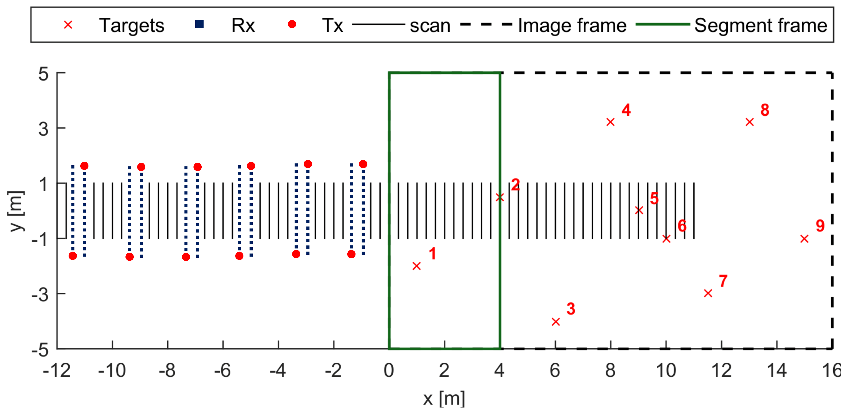
For each position of the moving platform, only one of the two transmitters is activated. By alternating between the left and right antennas from one platform position to the next, a full aperture comprising 32 receive channels is obtained from two consecutive platform positions or scans. The first position of the system on the surface is at $x=-12$ m and the last one at $x=11$ m, as shown in Figure 2. Since the system radiates and collects data along the x-direction with a discretized step of ${\delta }_x=0.33$ m, we have a total of 70 scans (represented in Figure 2 with black vertical lines). The ground is modeled as a non-dispersive and non-magnetic homogeneous medium with effective relative dielectric constant ${\epsilon }_{\mathrm{r}}=6$ and conductivity ${\sigma }_{\mathrm{d}}=10$ mS/m. A rough profile for the interface separating the upper and lower dielectric half-spaces is introduced and a statistical model is exploited to provide a realistic representation in the numerical code. The model is described by two functions [18]: the probability density function of the height variations and the surface autocorrelation function. For the numerical data considered in this paper, a 2-D zero-mean surface profile represented by Gaussian statistics (described by two parameters: the $rms$ height $h_{\mathrm{rms}}$ and the correlation length $l_c$) is assumed. Thus, the scattered electric field is considered to be a random process and evaluated by means of a Monte Carlo simulation [18,40].

The investigation area (indicated by a black dashed rectangle in Figure 2 has dimensions of 10 m $\times 16$ m along y and x directions, respectively, and is populated by a total of nine targets at distinct locations. The target characteristics are summarized in

Table 2. Target characteristics.

Target No.	Type	State	Size
1	Metallic anti-personnel landmine	Buried	Diameter: 100 mm; Height: 55 mm
2	Plastic anti-personnel landmine	On surface	Diameter: 100 mm; Height: 55 mm
3	Metallic artillery shell	Buried	Diameter: 155 mm; Length: 585 mm
4	Metallic anti-tank landmine	Buried	Diameter: 300 mm; Height: 125 mm
5	Metallic anti-tank landmine	On surface	Diameter: 300 mm; Height: 125 mm
6	Metallic artillery shell	Buried	Diameter: 155 mm; Length: 585 mm
7	Metallic artillery shell	Buried	Diameter: 155 mm; Length: 585 mm
8	Plastic anti-personnel landmine	On surface	Diameter: 100 mm; Height: 55 mm
9	Plastic anti-tank landmine	Buried	Diameter: 300 mm; Height: 125 mm

.

Buried targets are positioned 3 cm below the surface. The plastic targets have a relative dielectric constant ${\epsilon }_{\mathrm{r}}=3.1$ and conductivity $\sigma =2$ mS/m. For the rough ground surface, $h_{\mathrm{rms}}=1.6$ cm and $l_c=14.26$ cm. The characteristics of the investigation area are summarized in Table 1.

3.2. Image Formation Results

In order to maintain a similar cross-range resolution over the entire image, the investigation area is divided into four segments, each of dimension 10 m $\times 4$ m. The first segment is highlighted in Figure 2 with a green rectangle. Since coherent integration has been shown to reduce clutter [31], we coherently add multiple images of each segment generated with measurements from a set of full apertures using the MF-based tomographic algorithm detailed in Section 2.1. The CF-based processing of Section 2.3 is then applied to the resulting composite image. The set of apertures for each segment are selected so that the standoff distances are the same across all the image segments. Instead of choosing consecutive apertures for each segment, we opt for a set of apertures wherein any two neighboring apertures are separated by $4{\delta }_x=4\left(0.33\right)=1.32$ m, with the aperture closest to the segment at a standoff distance of 1 m. Figure 2 and Figure 3 depict the respective sets of full apertures used for the first and the last segments (indicated as blue dashed vertical lines). Such a choice provides a larger variation of the clutter across the various images being combined. For more details on the coherent combining procedure, see [14].

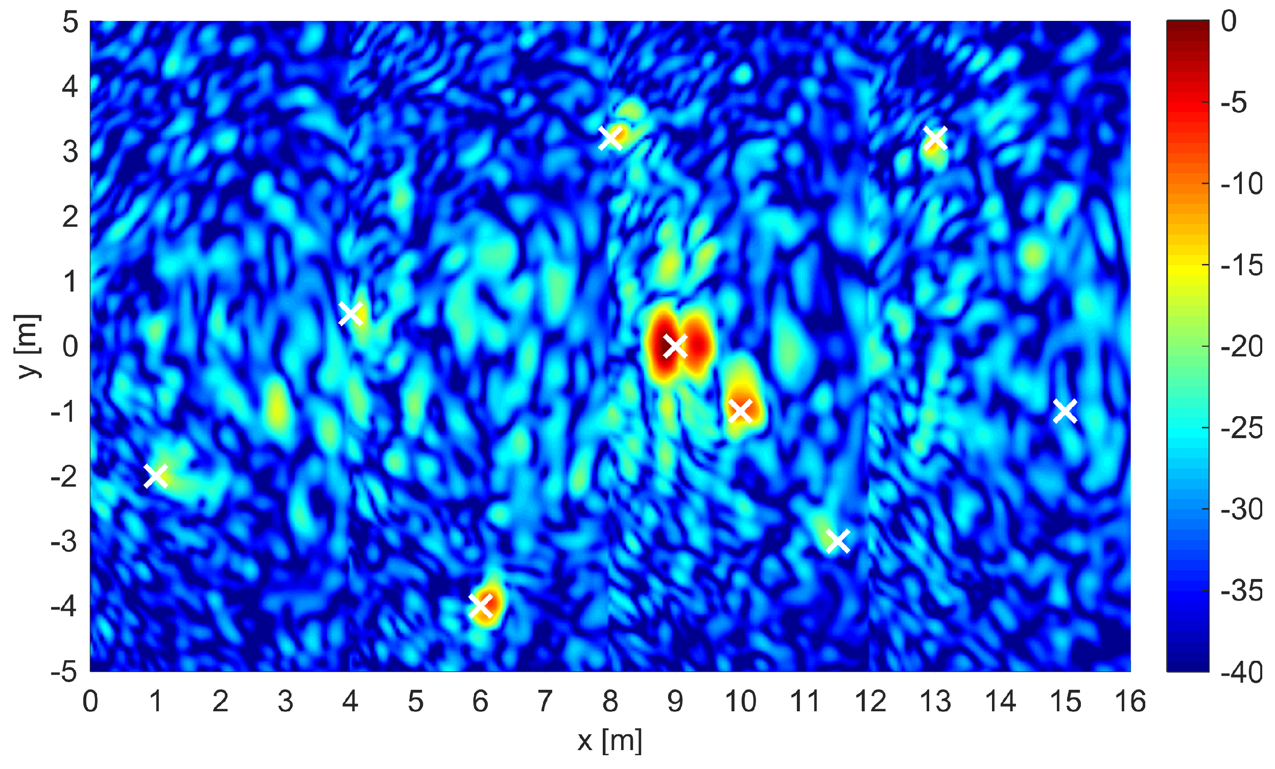
In Figure 4, we present the MF-based composite image corresponding to two full apertures (ones closest to each segment), whereas that corresponding to six full apertures is depicted in Figure 5. These results and all subsequent images in this paper are plotted on a 40 dB dynamic range, unless otherwise stated, with the maximum intensity value in each image normalized to 0 dB. The target positions are indicated with white crosses in both Figure 4 and Figure 5. The clutter generated by the rough surface dominates the image in Figure 4 and obscures the low-signature targets. Owing to the integration of a larger number of apertures permitted by the considered FL-GPR configuration, the clutter in Figure 5 is reduced as compared to Figure 4. Nonetheless, there is still substantial residual clutter in Figure 5, which would render target detection challenging. This demonstrates the need for further enhancements via the proposed CF procedure.

For comparison, we provide in Figure 6 and Figure 7 the images obtained by exploiting the same apertures as in Figure 4 and Figure 5, but with a BP algorithm [1]. As expected, the coherent combining of six full apertures allows for higher clutter suppression. Comparing the MF-based images with their respective BP counterparts, the improvements offered by the more accurate vector model adopted by the MF tomographic algorithm over the scalar-model-based BP algorithm are clearly visible in the central part of the images, where the clutter manifests itself as relatively weaker in strength. These qualitative observations are also validated by the corresponding SCR values, listed in

Table 3. Signal-to-clutter ratio (SCR) for back-projected and matched-filtering (MF)-based tomographic images.

	Figure Number	SCR (dB)
MF 2 apertures	Figure 4	−7.4
MF 6 apertures	Figure 5	−0.4
BP 2 apertures	Figure 6	−8.7
BP 6 apertures	Figure 7	−3.3

. More specifically, the MF algorithm provides an improvement of 1.3 dB and 2.9 dB over the BP algorithm for the 2- and 6-apertures cases, respectively.

3.3. CF Enhanced Results

We first apply the enhancement procedure based on ACF to both MF and BP images, and demonstrate the superior clutter suppression capability yielded by the MF-based ACF over that defined using the scalar-model-based BP algorithm.

Figure 8 depicts the image obtained by means of the ACF-based masking operation applied to the two-aperture MF image of Figure 4. The image enhancements in terms of clutter mitigation are clearly visible with respect to the original. Figure 9 shows the two-aperture BP image of Figure 6 after the BP-based ACF masking operation was applied. Comparing Figure 8 and Figure 9, we observe that the MF-based enhancement procedure provides a higher degree of clutter suppression. The six-aperture MF and BP images after application of the ACF-based correction are shown in Figure 10 and Figure 11, respectively. As expected, more clutter has been suppressed with respect to the two-aperture configuration for both cases. Similar to the two-apertures case, the MF-based definition of the ACF provides a cleaner image, which would lead to an improved detection performance.

Having demonstrated the superiority of the MF-based proposed procedure over the BP-based enhancement, we next compare and contrast the performance of the CF-based scheme when ACF, PCF, and SCF are individually used to generate the coherence maps for clutter suppression in MF images. We consider the MF image of Figure 5 (six-aperture case) for this purpose. Figure 12 and Figure 13 present the resulting images after application of the clutter suppression procedure via PCF and SCF, respectively. Comparing Figure 12 and Figure 13 with the ACF corrected image of Figure 10, we observe that the different coherence map definitions provide comparable degree of clutter suppression. This is also demonstrated by the corresponding SCR values, provided in

Table 4. SCR for six-aperture images after CF-based enhancement.

	Figure Number	SCR (dB)
ACF MF	Figure 10	6.7
ACF BP	Figure 11	5.6
PCF MF	Figure 12	7.0
SCF MF	Figure 13	7.6

. More specifically, all three variants of CF provide SCR improvements of 7 to 8 dB over the original image of Figure 5. Similar results were obtained when the three variants of the CF were applied to the MF image obtained through the coherent combining of two apertures.

4. Discussion

The qualitative and quantitative results of Section 3 clearly demonstrated the superior performance of the CF clutter suppression approach based on MF image formation over its BP-based counterpart. This superiority is attributed to the high-accuracy vector model employed by the MF algorithm over the scalar-model-based BP algorithm. Further, coherent integration of measurements from multiple full apertures should be employed, whenever possible, in conjunction with the CF-based approach for a higher degree of clutter suppression. Furthermore, performance evaluation of different coherence map definitions, namely, ACF, PCF, and SCF, showed that all three variants of CF provide comparable levels of clutter suppression. In terms of the impact of the CF-based processing on the target regions, we observed that both ACF and PCF had a minimal effect, as evident from Figure 10 and Figure 12. However, each target region in the SCF-corrected image split up into multiple lobes, as evident in Figure 13, which may be problematic for subsequent target detection schemes. Finally, we note that target 9 did not survive the clutter suppression process and was missing from all CF-corrected results reported in Section 3. This is because the target in question is the only plastic target buried in the ground. Buried plastic targets are especially hard to detect due to (i) the limited dielectric contrast between the target and the soil background, and (ii) interference from rough surface scattering. This observation is consistent with what has been previously reported in the literature [31].

5. Conclusions

In this paper, we proposed a matched filtering formulation of tomographic near-field imaging and presented a coherence-factor-based rough surface clutter mitigation technique for FL-GPR imaging. The CF was used to generate a coherence map, which was then applied as a correction mask to the microwave image. Improvements achievable, in terms of reduction of the incoherent component produced by the rough surface with respect to coherent scattering from targets, were assessed using numerical data of metallic and plastic targets both on-surface and buried at shallow depths. The performance of the proposed scheme was also quantified by evaluating the improvements in image-domain SCR and contrasted with that obtained using a standard back-projection imaging algorithm. The proposed approach was shown to outperform the back-projection-based scheme. Different definitions of the CF were considered and compared. It was shown that the three variants of the CF all yielded comparable but excellent SCR enhancements. While the SCF generated some artifacts by splitting each target into multiple lobes, both the ACF and PCF exhibited minimal impact on the weak target signatures.

References

- Pastorino, M. Microwave Imaging; John Wiley & Sons Inc.: Hoboken, NJ, USA, 2010. [Google Scholar]
- Jin, S.; Haghighipour, N.; Ip, W.-H. (Eds.) Planetary Exploration and Science: Recent Results and Advances; Springer: Berlin/Heidelberg, Germany, 2015. [Google Scholar]
- Amin, M.G. Through-the-Wall Radar Imaging; CRC Press: Boca Raton, FL, USA, 2011. [Google Scholar]
- Solimene, R.; Catapano, I.; Gennarelli, G.; Cuccaro, A.; Dell Aversano, A.; Soldovieri, F. SAR imaging algorithms and some unconventional applications. IEEE Signal Process. Mag. 2014, 31, 90–98. [Google Scholar] [CrossRef]
- Persico, R. Introduction to Ground Penetrating Radar: Inverse Scattering and Data Processing; John Wiley & Sons Inc.: Hoboken, NJ, USA, 2014. [Google Scholar]
- Lo Monte, L.; Erricolo, D.; Soldovieri, F.; Wicks, M.C. Radio frequency tomography for tunnel detection. IEEE Trans. Geosci. Remote Sens. 2010, 48, 1128–1137. [Google Scholar] [CrossRef]
- Garcia-Fernandez, M.; Morgenthaler, A.; Alvarez-Lopez, Y.; Las Heras, F.; Rappaport, C. Bistatic landmine and IED detection combining vehicle and drone mounted GPR sensors. Remote Sens. 2019, 11, 2299. [Google Scholar] [CrossRef] [Green Version]
- Kositsky, J.; Cosgrove, R.; Amazeen, C.; Milanfar, P. Results from a forward-looking GPR mine detection system. Proc. SPIE 2002, 4742, 206–217. [Google Scholar]
- Kositsky, E.M.; Rotondo, F.S.; Elizabeth, A. Testing and evaluation of forward-looking GPR countermine systems. Proc. SPIE 2005, 5794, 901–911. [Google Scholar]
- Wang, Y.; Sun, Y.; Li, J.; Stoica, P. Adaptive imaging for forward-looking ground penetrating radar. IEEE Trans. Aerosp. Electron. Syst. 2005, 41, 922–936. [Google Scholar] [CrossRef]
- Wang, T.; Keller, J.M.; Gader, P.D.; Sjahputera, O. Frequency sub-band processing and feature analysis of forward-looking ground penetrating radar signals for land-mine detection. IEEE Trans. Geosci. Remote Sens. 2007, 45, 718–729. [Google Scholar] [CrossRef]
- Soldovieri, F.; Gennarelli, G.; Catapano, I.; Liao, D.; Dogaru, T. Forward-looking radar imaging: A comparison of two data processing strategies. IEEE J. Sel. Top. Appl. Earth Obs. Remote Sens. 2017, 10, 562–571. [Google Scholar] [CrossRef]
- Ogworonjo, H.C.; Anderson, J.M.M.; Nguyen, L.H. An iterative parameter-free MAP algorithm with an application to forward looking GPR imaging. IEEE Trans. Geosci. Remote Sens. 2017, 55, 1573–1586. [Google Scholar] [CrossRef]
- Comite, D.; Ahmad, F.; Liao, D.; Dogaru, T.; Amin, M.G. Multiview imaging for low-signature target detection in rough-surface clutter environment. IEEE Trans. Geosci. Remote Sens. 2017, 55, 5220–5229. [Google Scholar] [CrossRef]
- Catapano, I.; Affinito, A.; Del Moro, A.; Alli, G.; Soldovieri, F. Forward-looking ground-penetrating radar via a linear inverse scattering approach. IEEE Trans. Geosci. Remote Sens. 2015, 53, 5624–5633. [Google Scholar] [CrossRef]
- Sun, Y.; Li, J. Time-frequency analysis for plastic landmine detection via forward-looking ground penetrating radar. Proc. Inst. Elect. Eng. Radar Sonar Navig. 2003, 150, 253–261. [Google Scholar] [CrossRef]
- Nguyen, L. SAR imaging technique for reduction of sidelobes and noise. Proc. SPIE 2009, 7308, 73080U. [Google Scholar]
- Liao, D.; Dogaru, T.; Sullivan, A. Large-scale, full-wave-based emulation of step-frequency forward-looking radar imaging in rough terrain environments. Sens. Imag. 2014, 15, 88. [Google Scholar] [CrossRef]
- Ton, T.; Wong, D.; Soumekh, M. ALARIC forward-looking ground penetrating radar system with standoff capability. In Proceedings of the 2010 IEEE International Conference on Wireless Information Technology and Systems, Honolulu, HI, USA, 8 August–3 September 2010. [Google Scholar]
- Yang, J.; Jin, T.; Huang, X.; Thompson, J.; Zhou, Z. Sparse MIMO array forward-looking GPR imaging based on compressed sensing in clutter environment. IEEE Trans. Geosci. Remote Sens. 2014, 52, 4480–4494. [Google Scholar] [CrossRef]
- Tajdini, M.M.; Gonzalez-Valdes, B.; Martinez-Lorenzo, J.A.; Morgenthaler, A.W.; Rappaport, C.M. Real-time modeling of forward-looking synthetic aperture ground penetrating radar scattering from rough terrain. IEEE Trans. Geosci. Remote Sens. 2019, 57, 2754–2765. [Google Scholar] [CrossRef]
- Comite, D.; Ahmad, F.; Dogaru, T.; Amin, M.G. Adaptive detection of low-signature targets in forward-looking GPR imagery. IEEE Geosci. Remote Sens. Lett. 2018, 15, 1520–1524. [Google Scholar] [CrossRef]
- Pambudi, A.D.; Fauss, M.; Ahmad, F.; Zoubir, A.M. Robust detection for forward-looking GPR in rough-surface clutter environments. In Proceedings of the 52nd Asilomar Conference on Signals, Systems, and Computers, Pacific Grove, CA, USA, 28–31 October 2018; pp. 2077–2080. [Google Scholar]
- Keller, S.K.; Ho, K.C.; Busch, M.; Gader, P.D. On the registration of FLGPR and IR data for a forward-looking landmine detection system and its use in eliminating FLGPR false alarms. Proc. SPIE 2008, 6953, 695314. [Google Scholar]
- Li, L.; Zhang, W.; Li, F. Derivation and discussion of the SAR migration algorithm within inverse scattering problem: Theoretical analysis. IEEE Trans. Geosci. Remote Sens. 2010, 48, 415–422. [Google Scholar]
- Gilmore, C.; Jeffrey, I.; Lo Vetri, J. Derivation and comparison of SAR and frequency-wavenumber migration within a common inverse scalar wave problem formulation. IEEE Trans. Geosci. Remote Sens. 2006, 44, 1454–1461. [Google Scholar] [CrossRef]
- Leuschen, C.J.; Plumb, R.G. A matched-filter-based reverse-time migration algorithm for ground-penetrating radar data. IEEE Trans. Geosci. Remote Sens. 2001, 39, 929–936. [Google Scholar] [CrossRef] [Green Version]
- Hollman, K.W.; Rigby, K.W.; O Donnell, M. Coherence factor of speckle from a multi-row probe. In Proceedings of the 1999 IEEE Ultrasonics Symposium, Caesars Tahoe, NV, USA, 17–20 October 1999; pp. 1257–1260. [Google Scholar]
- Klemm, M.; Leendertz, J.A.; Gibbins, D.; Craddock, I.J.; Preece, A.; Benjamin, R. Microwave radar-based breast cancer detection: Imaging in inhomogeneous breast phantoms. IEEE Antennas Wireless. Prop. Lett. 2009, 8, 1949–1952. [Google Scholar] [CrossRef] [Green Version]
- Burkholder, R.J.; Browne, K.E. Coherence factor enhancement of through-wall radar images. IEEE Antennas Wirel. Prop. Lett. 2010, 9, 842–845. [Google Scholar] [CrossRef]
- Liao, D.; Dogaru, T. Full-wave characterization of rough terrain surface scattering for forward-looking radar applications. IEEE Trans. Antennas Propag. 2012, 60, 3853–3866. [Google Scholar] [CrossRef]
- Comite, D.; Ahmad, F.; Dogaru, T.; Amin, M.G. Coherence factor for rough surface clutter mitigation in forward-looking GPR. In Proceedings of the 2017 IEEE Radar Conference (RadarConf), Seattle, WA, USA, 8–12 May 2017; pp. 1803–1806. [Google Scholar]
- Li, S.; Amin, M.; An, Q.; Zhao, G.; Sun, H. 2-D coherence factor for sidelobe and ghost suppressions in radar imaging. IEEE Trans. Antennas Propag. 2019, 68, 1204–1209. [Google Scholar] [CrossRef] [Green Version]
- Chew, W.C. Waves and Fields in Inhomogeneous Media; Wiley-IEEE Press: Hoboken, NJ, USA, 1995. [Google Scholar]
- Lu, B.Y.; Sun, X.; Zhao, Y.; Zhou, Z.M. Phase coherence factor for mitigation of sidelobe artifacts in through-the-wall radar imaging. J. Electromagn. Waves Appl. 2013, 27, 716–725. [Google Scholar] [CrossRef]
- Camacho, J.; Parrilla, M.; Fritsch, C. Phase coherence imaging. IEEE Trans. Ultrason. Ferroelectr. Freq. Control 2009, 56, 958–974. [Google Scholar] [CrossRef]
- Liu, J.; Jia, Y.; Kong, L.; Yang, X.; Liu, Q.H. Sign-coherence-factor-based suppression for grating lobes in through-wall radar imaging. IEEE Geosci. Remote Sens. Lett. 2016, 13, 1681–1685. [Google Scholar] [CrossRef]
- Yoon, Y.S.; Amin, M.G. Spatial filtering for wall-clutter mitigation in through-the-wall radar imaging. IEEE Trans. Geosci. Remote Sens. 2009, 47, 3192–3208. [Google Scholar] [CrossRef]
- Adams, R.; Bischof, L. Seeded region growing. IEEE Trans. Pattern Anal. Mach. Intell. 1994, 16, 64–647. [Google Scholar] [CrossRef] [Green Version]
- Chan, C.H.; Tsang, L. Monte Carlo simulations of large-scale one-dimensional random rough-surface scattering at near-grazing incidence: Penetrable case. IEEE Trans. Antennas Propag. 1998, 46, 142–149. [Google Scholar] [CrossRef]
Figure 1.
Side-view of the forward-looking ground-penetrating radar (FL-GPR) configuration and data collection geometry.
Figure 2.
Top view of the numerical simulation geometry. Six different full-aperture measurements have been highlighted in blue, which are used in coherent combining for the first image segment indicated in green (the positions of transmitters and receivers are not drawn to scale within the image frame).
Figure 3.
The last image segment is highlighted in green and the relevant full aperture measurements to be exploited in coherent combining are indicated in blue (the positions of transmitters and receivers are not drawn to scale within the image frame).
Figure 4.
Image obtained by integrating two apertures for the scene containing nine targets and a rough surface ( cm). The true position of targets is indicated with a white cross.
Figure 5.
Image obtained by integrating six apertures for the same scene as in Figure 4.
Figure 6.
Image as in Figure 4, but generated through the back-projection (BP) algorithm.
Figure 7.
Image as in Figure 5, but obtained by means of the BP algorithm.
Figure 8.
MF based image of Figure 4 after application of the ACF-based enhancement procedure. The target position and type are indicated with a white cross and number.
Figure 9.
BP image of Figure 6 after application of the amplitude coherence factor (ACF)-based enhancement procedure. The target position and type are indicated with a white cross and number.
Figure 10.
MF image of Figure 5 after ACF based enhancement.
Figure 11.
BP image of Figure 7 after ACF based enhancement.
Figure 12.
MF Image of Figure 5 corrected via phase coherence factor (PCF).
Figure 13.
MF image of Figure 5 corrected via sign coherence factor (SCF).