Article

A Multi-Scale Superpixel-Guided Filter Feature Extraction and Selection Approach for Classification of Very-High-Resolution Remotely Sensed Imagery

1
College of Surveying and Geoinformatics, Tongji University, Shanghai 200092, China
2
Geoinformatics Unit, RIKEN Center for Advanced Intelligence Project, Tokyo 103-0027, Japan
3
Department of Electrical and Computer Engineering, Mississippi State University, Starkville, MS 39762, USA
4
Xinjiang Institute of Ecology and Geography, CAS and the CAS Research Center for Ecology and Environment of Central Asia, Urumqi 830011, China
5
Institute of Cartography and Geographic Information System, Chinese Academy of Surveying and Mapping, Beijing 100830, China
*
Author to whom correspondence should be addressed.
Submission received: 29 January 2020 / Revised: 2 March 2020 / Accepted: 5 March 2020 / Published: 7 March 2020
(This article belongs to the Special Issue Multi-Modality Data Classification: Algorithms and Applications)

Abstract

:
In this article, a novel feature selection-based multi-scale superpixel-based guided filter (FS-MSGF) method for classification of very-high-resolution (VHR) remotely sensed imagery is proposed. Improved from the original guided filter (GF) algorithm used in the classification, the guidance image in the proposed approach is constructed based on the superpixel-level segmentation. By taking into account the object boundaries and the inner-homogeneity, the superpixel-level guidance image leads to the geometrical information of land-cover objects in VHR images being better depicted. High-dimensional multi-scale guided filter (MSGF) features are then generated, where the multi-scale information of those land-cover classes is better modelled. In addition, for improving the computational efficiency without the loss of accuracy, a subset of those MSGF features is then automatically selected by using an unsupervised feature selection method, which contains the most distinctive information in all constructed MSGF features. Quantitative and qualitative classification results obtained on two QuickBird remotely sensed imagery datasets covering the Zurich urban scene are provided and analyzed, which demonstrate that the proposed methods outperform the state-of-the-art reference techniques in terms of higher classification accuracies and higher computational efficiency.

Graphical Abstract

1. Introduction

In the last few decades, the quick development of the advanced remote sensing satellite sensors has enabled the acquisition of remotely sensed imageries with increasing higher spatial resolution. The numerous VHR data lead to its successful utility in different practical applications. In particular, this allows the land surface type classification at a very fine scale. VHR imageries are often characterized by rich texture and structural information, but also by few relatively limited spectral bands. Although small land-cover objects with more details might be detected more precisely owing to the abundant spatial descriptions, this may still lead to the existence of isolate noises (“salt and pepper” phenomenon) during the classification process [1]. Besides, the insufficient spectral bands and uncertain spectral variations may also result in poor results with low classification performance. This is because of the spectral variability among or within land-covers with different types having similar spectra or the same type having dissimilar object spectra [2,3].
In order to alleviate the aforementioned phenomenon and improve the VHR images’ classification performance, many literature works are devoted to exploiting the image object geometrical and spatial information in classification. Recent advances in object-oriented-based methods have provided an efficient way to improve classification results. These methods usually group spatially adjacent pixels into spectrally homogeneous small regions, where the classification is then directly carried out on the segmented objects or they optimize the pixel level classification maps by constraining the segmented object edges. Tarabalka et al. [4] utilized watershed transformation and clustering to generate segments (individual objects). Features such as mean values of the spectral and spatial measurements of the objects were extracted as the input of a classifier to implement object-based classification. Csillik [5] implemented a fast image segmentation and classification of VHR remotely sensed imagery relying on the segmented superpixels. However, as the final classification result depends on the segmentation performance, which is sensitive to the scale selection [6,7,8], several literature were devoted to seeking such a best segmentation scale. For instance, Drǎguţ et al. [9] estimated the scale parameter in the object-based image analysis using the idea of the local variance of object heterogeneity in a scene. Hu et al. [7] developed a stepwise evolution analysis framework to analyze the optimal scale parameter in the region-merging segmentation. While such object-oriented-based methods can partly remove “salt and pepper” noise, accurate object identification in VHR images is still a challenging problem due to the variation of the features and the proper selection of an effective segmentation strategy. Rather than an object-based method, pixel-by-pixel approaches with spatial features such as the gray level co-occurrence matrix (GLCM), the wavelet transformation (WT), and the morphology profiles (MP) represent another major family for addressing the classification problem in VHR images. For instance, Monika et al. [10] explored the utility of the GLCM variance to discriminate slums and formal built-up areas in VHR images. Chen et al. [11] used multi-resolution WT to achieve high-frequency information for representing spatial characteristics of the built-up areas at different scales. MP is one of the most popular methods as its capability of weakening some local spatial details and simultaneously preserving the structural information of the other regions. Bellens et al. [12] extracted spatial features with two MPs based on linear-shaped and disk-shaped structure elements to preserve the shape of the objects. Samat et al. [13] introduced maximally stable extremal region-guided MPs to implement spatial feature extraction by adaptively setting structure elements, which matched all image objects with respect to their size and shape. Though the aforementioned approaches have been validated to be effective in literature works, they still have some limitations. Features extracted by those methods are always high-dimensional with the process of moving windows or a series of mathematical operations at different scales, which inevitably produces redundancy and results in the increase of the computational complexity [12,14,15,16].
To solve this problem, a subset of a high-dimensional feature set can be selected to perform classification in a more efficient way. Two major clusters including feature transformation approaches (e.g., principal component analysis [17], independent component analysis [18], and minimum noise fraction [19]) and feature selection approaches have been intensively investigated. The former is able to reduce the original data dimensionality into a low-dimensional space via data transformation, but with the loss of the physical meaning of the features. The latter can be implemented with a selection of the most informative portion of the whole feature space with high dimensionality. This is realized either in an unsupervised or supervised manner according to a certain criterion and a search strategy. Supervised methods usually require the desired object to be known a priori. For instance, statistical distance measurements like Bhattacharyya distance [20], Jeffries–Matusita (J-M) distance [21], and transformed divergence measure [22] are often used as selection criteria to assess the separability of a given feature subset. Although these supervised approaches provide better performance in classification or detection than unsupervised ones, the ground reference data are often unavailable in practical cases. In this context, unsupervised methods mainly implement the feature selection in a ranking, clustering, or optimization manner, which makes it more feasible in practical applications. For example, Du et al. [23] employed the concept of endmember extraction in the band selection algorithm based on bands’ similarity. Jia et al. [24] proposed an enhanced fast density-peak-based clustering (E-FDPC) method in selecting bands by applying an exponential-based learning rule on the original FDPC algorithm. Tschannerl et al. [25] used the criterion of “maximum information minimum redundancy” to generate the subset with a modified discrete gravitational search method. All these methods reduce the feature dimensionality and thus the computational time cost, while keeping the performance of the classification or detection task to a great extent.
In the past decade, edge-preserving filtering such as the guided filter (GF) has proven to be effective in different image processing applications, for example in image smoothing/enhancement, image fusion [26], dehazing [27], image segmentation [28], saliency detection [29], etc. Theoretically, considering the spatial representation of a guidance image, GF is capable of transferring the intrinsic properties of the guidance image, especially its structures, to a filtered output, which can smooth the noise probabilities, but also preserve the real object boundary in the filtered image [30]. In the literature, GF is mainly introduced and applied in the classification of hyperspectral data. Kang et al. [31] developed a single-scale GF method to investigate the output classification probabilities with local optimization. Wang et al. [32] proposed a multi-scale classification approach by taking advantage of the pixel-wise GF. Despite the aforementioned literature works, to the best of our knowledge, GF and its modified versions have not been further analyzed in detail in the VHR image classification task. In this case, the rich spatial feature information could better represent land-cover objects, whose class boundaries and inner-homogeneity are both very important ingredients for producing an accurate classification map. Motivated by this, a novel classification approach for VHR images by using the feature selection-based multi-scale superpixel GF features is proposed in this study. The main novelty and contributions of this work are summarized as follows: (1) we propose a novel feature selection-based multi-scale superpixel-based guided filter (FS-MSGF) method for dealing with the VHR imagery classification problem; (2) we modify and improve the original pixel-level GF into a superpixel-level version, where a superpixel-level guidance image can provide more accurate boundary information of the image objects and internal spectral homogenous information of each segment; (3) we consider the multi-scale GF feature information in the classification rather than the single-scale feature as in the GF literature works; (4) an unsupervised feature selection algorithm is utilized on the high-dimensional multi-scale feature sets to extract the most informative features and largely reduce the computational cost, but maintaining the accuracy at a high level.
The rest of the paper is organized as follows. Section 2 introduces the VHR datasets used and describes in detail the proposed FS-MSGF method. Experimental results and discussions are provided in Section 3 and Section 4, respectively. Finally, in Section 5, we draw the conclusion.

2. Materials and Methods

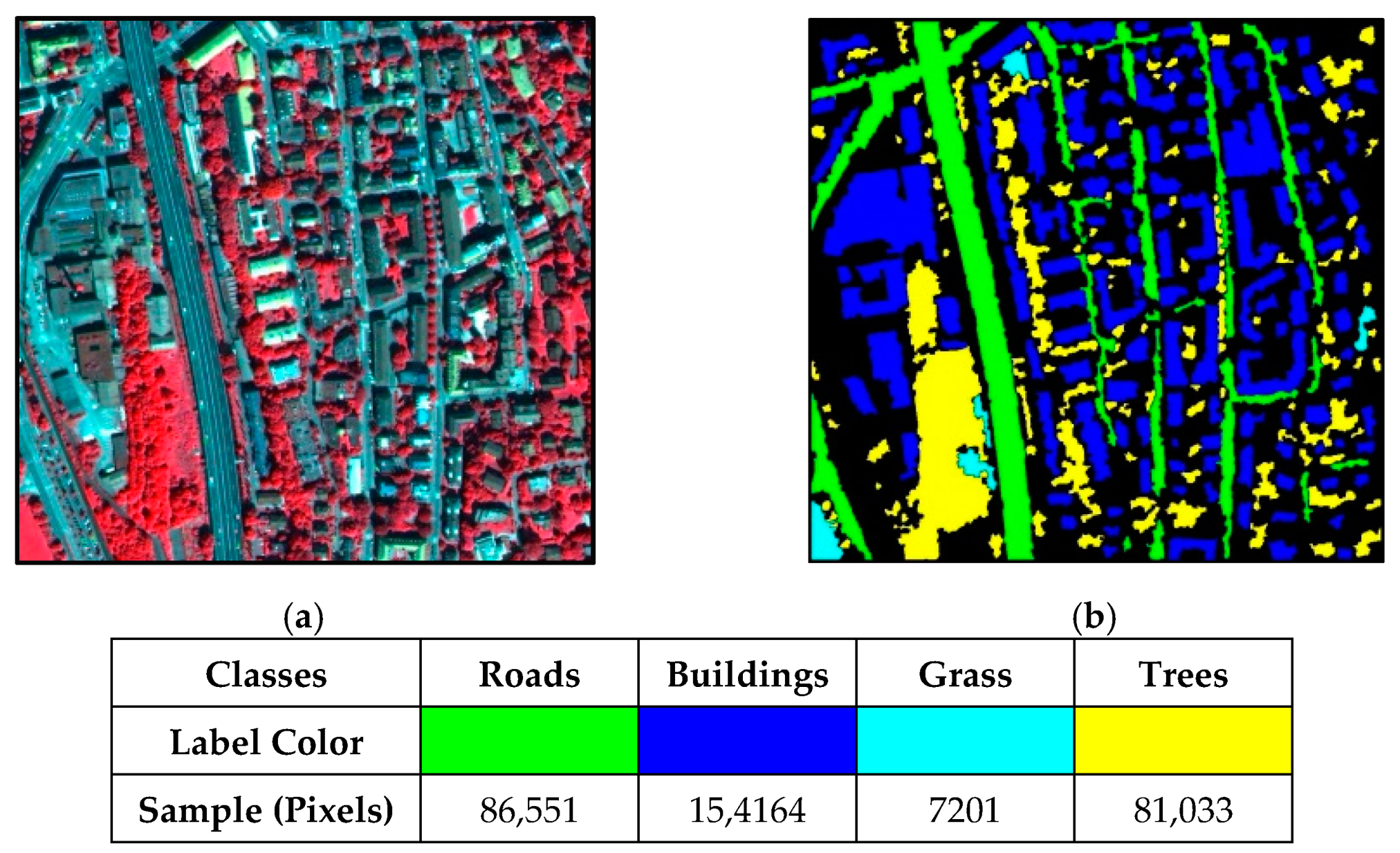
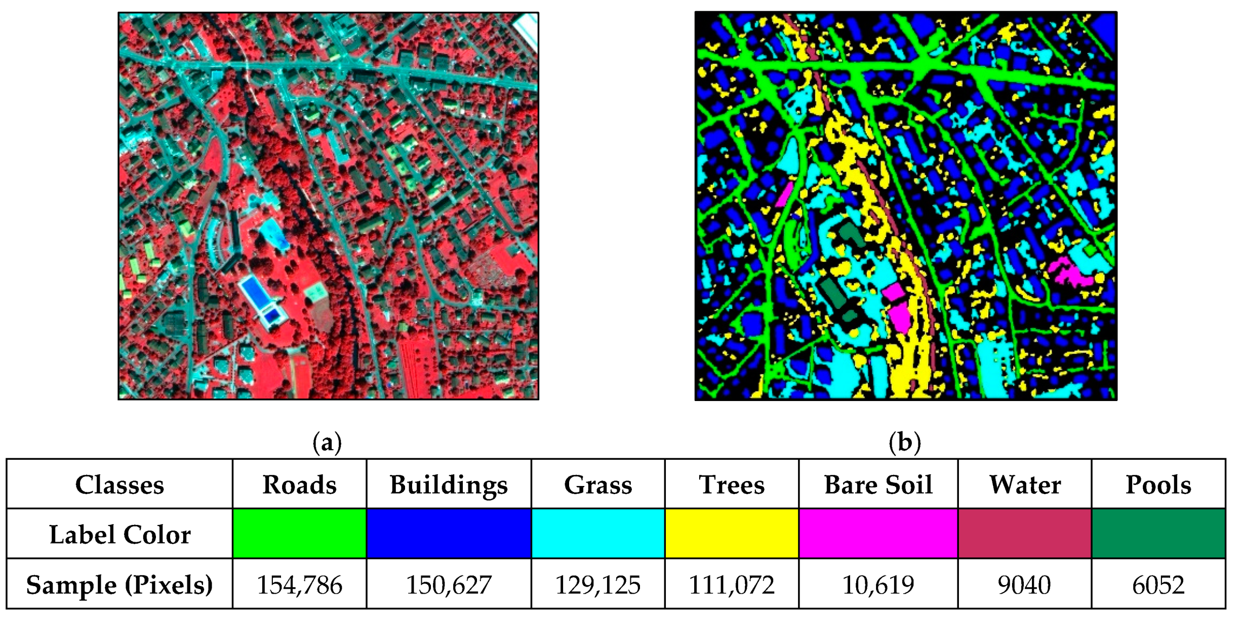
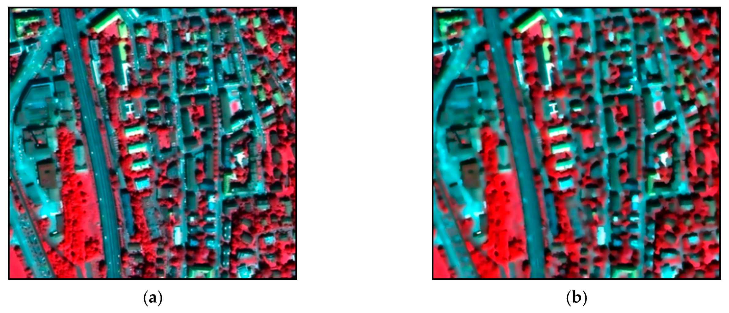
2.1. VHR Remote Sensing Datasets

Experiments in this work were conducted on two VHR remotely sensed imageries acquired by the QuickBird satellite covering an urban area in Zurich, Switzerland, in August 2002. Zurich Dataset 1 and Zurich Dataset 2 (denoted as “Zh1” and “Zh2” in the following sections) had a size of 833×881 pixels and 1025×1112 pixels, respectively. The Gram–Schmidt (G-S) pan-sharpening fusing operation was performed to combine the panchromatic and multispectral bands to generate four fused bands (visible red, green, blue, and also, near-infrared) having a spatial resolution of approximately 0.62 meters. For more details about the Zurich dataset, the reader can refer to https://sites.google.com/site/michelevolpiresearch/data/zurich-dataset. Four land-cover types including buildings, grass, trees, and roads in Zh1 and seven classes (i.e., trees, buildings, roads, grass, bare soil, water, and pool) in Zh2 are available in the reference maps. Figure 1a and Figure 2a show the images of two datasets and the corresponding available reference maps. Training and testing samples used in the experiments are provided in detail in Table 1, where 1% and 0.5% of the whole available samples were used as training samples and the rest for testing on the two datasets, respectively.

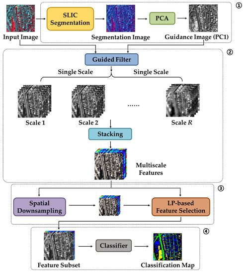
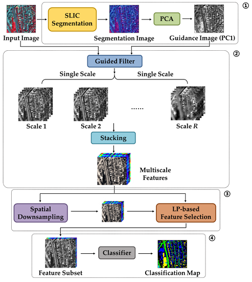
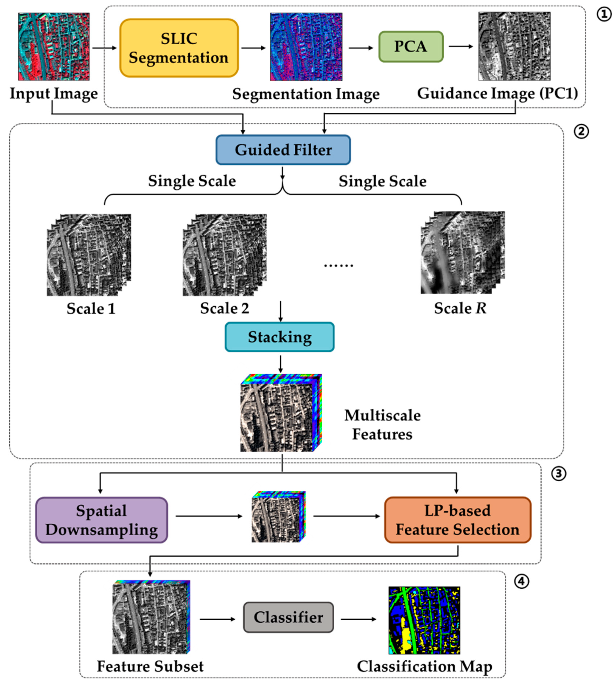
2.2. Proposed Method

In this study, to complete the VHR image classification task over the complex urban scene, a novel feature selection-based multi-scale superpixel guided filter (FS-MSGF) approach is proposed. The proposed FS-MSGF method consisted of the following four main steps: ① superpixel segmentation for building the guidance image; ② multi-scale superpixel-guided filter feature generation; ③ unsupervised feature selection; and ④ classification relying on the selected MSGF feature subset. The whole flowchart of the proposed classification technique in this work is illustrated in Figure 3. More details are provided in the following subsections.

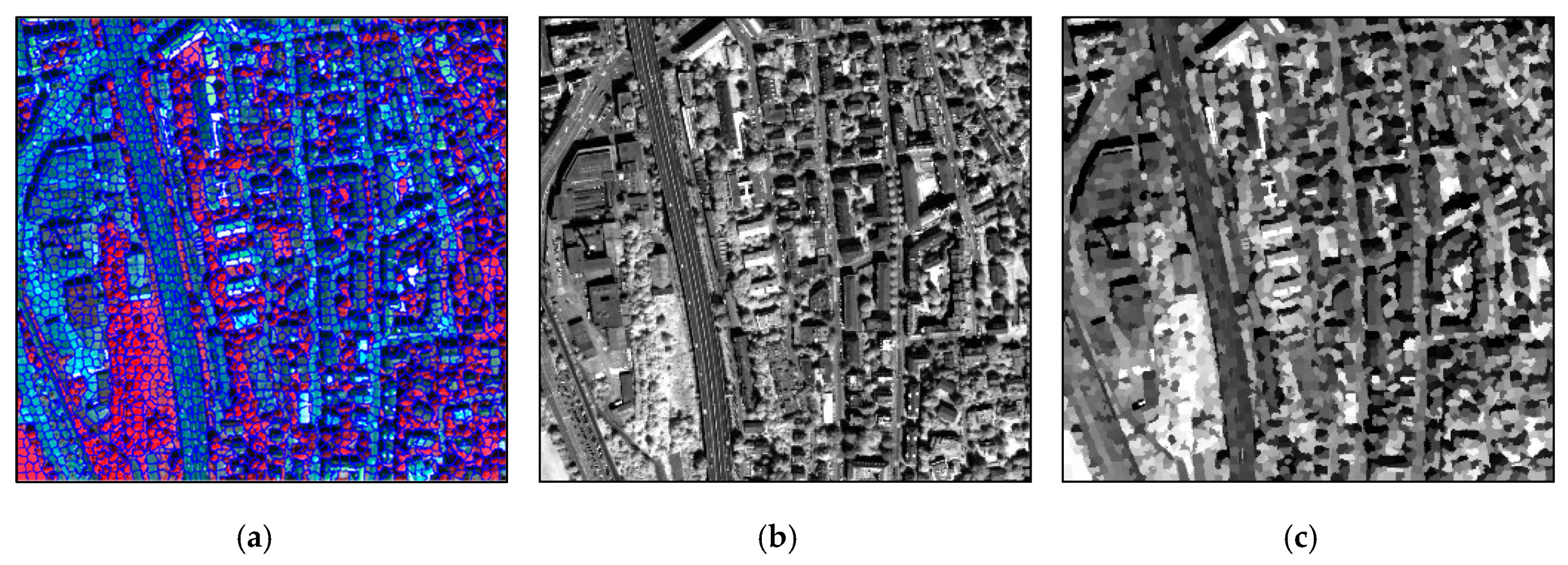
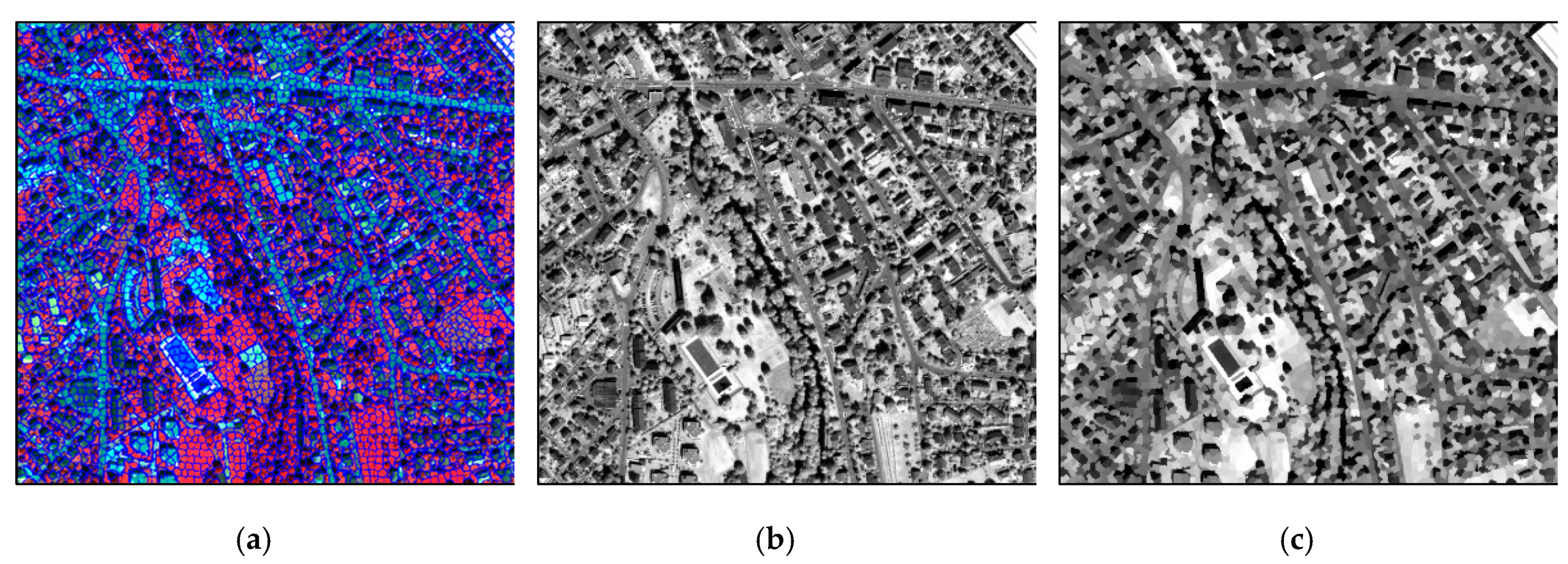
2.2.1. Superpixel Segmentation for Building the Guidance Image

The aim of this step is to generate a suitable guidance image in the GF algorithm and use it for guiding the feature extraction in the next operations. Since the context of the guidance image is transferred to the filtering output by GF, we constructed a superpixel segmented map as the guidance image rather than the original pixel-wise one. By doing this, we expected that the geospatial land-cover objects in VHR imagery and internal consistence information of each segment could be depicted in a more precise manner. The SLIC (simple linear iterative clustering) algorithm was used [33] to accomplish this task due to its advantages of simplicity, boundary adherence, and high computational efficiency. The principle of the SLIC algorithm is to generate regional clusters using k-means, whose local homogeneity is considered in the CIELAB color space. Note that the segmentation in this study was conducted on the composite image with the near-infrared, red, and green bands. We selected them as most informative bands by calculating the global entropy index on all four bands, where these ones were the three having the highest entropy values in both datasets. The generated superpixel number, K, is defined according to the sampling interval of the clustering centroids S:
S = N / K
N represents the total pixels in the image. m represents an optional parameter that controls the compactness of the generated superpixels. The smaller m is, the more tightly superpixels adhere to the image boundary, leading to a less regular size and shape. Every pixel is then clustered to its nearest cluster center according to measurement D through the combination of two distances dc and ds:
d c = ( l β l α ) 2 + ( u β u α ) 2 + ( v β v α ) 2
d s = ( x β x α ) 2 + ( y β y α ) 2
D = ( d c m ) 2 + ( d s S ) 2
where dc and ds are the color and the two spatial distances between pixel-pair α and β. (x, y), (l, u, v) represent coordinates in the two spaces. Moreover, dc controls the spectral (color) homogeneity, whereas ds focuses on the compactness of spatially neighboring pixels, respectively.
Superpixel segmentation map is then obtained after the equalization of sample values within each segment. PCA is then performed on the segmented image. The final guidance image is built from the first principal component (PC1), which represents the majority descriptions for the image object information.

2.2.2. Multi-Scale Superpixel-Guided Filter Feature Generation

The main assumption of GF is given as follows: A local linear model can be assumed between a guidance image G and a filtered output image O, where O is modelled as a linear transform of G within a window ω having a size of (2r + 1) × (2r + 1). It can be described as [30]:
O i = a j G i + b j ,   i ω j
where Gi and Oi are the values of the ith pixel in the guidance and output image and ωj is the window around the central pixel j. Then, in each ωj, two linear coefficients aj and bj can be calculated by minimizing a following cost function as:
E ( a j , b j ) = i ω j [ ( a j G i + b j I i ) 2 + ε a j 2 ]
where ε is the regularization parameter penalizing large aj. Different aj and bj values estimated in different windows are averaged as aj and bj. We can calculate the final Oi image as:
O i = a ¯ j G i + b ¯ j
where a ¯ j = 1 | ω | i ω j a i and b ¯ j = 1 | ω | i ω j b i . By applying the filtering with the guidance image, those abrupt changes within local gradient regions are expected to be well preserved, whereas others are smoothed under the effects of different sizes of pre-set windows. Such effects can be seen from an illustrated example as shown in Figure 4 by using the QuickBird images.
The original image bands were filtered by the generated superpixel-level guidance image with different radius r to model the land-cover objects at multiple scales. Superpixel-guided filter (SGF) features with a series of r were stacked to build multi-scale superpixel-guided filter (MSGF) features:
SGF ( X t ) = { SGF 1 ( X t ) , SGF 2 ( X t ) , , SGF R ( X t ) } r = 1 , 2 , , R
MSGF = { SGF ( X 1 ) , SGF ( X 2 ) , , SGF ( X t ) } t = 1 , 2 , , T
where R is a given upper bound of the searching filtering radius range. MSGF is the stacking SGF features from all bands in X (i.e., T). Accordingly, the dimension of MSGF comes to T × R in total, which will be a large number after stacking all the multi-scale GF features.
It should be note that if multiple bands’ color information were taken into consideration, we could also construct the color version of the superpixel-level guidance image. However, after intensive experimental comparisons, we discovered that the final performance of the proposed approach by using the gray or color guidance images did not make a significant difference, but the former was more effective from the computational point of view. Therefore, the gray version of the superpixel-level guidance image was used for all experiments presented in this article.

2.2.3. Unsupervised Feature Selection

Though features with multi-scale information were able to improve the representation of the land objects and thus promote the classification performance, a mass of redundant information might still simultaneously exist in the stacked high-dimensional MSGF features, which may bring about the increase of computational cost. Therefore, an unsupervised similarity-based feature selection [23] algorithm was adopted to find the most representative and distinctive subsets from the original features, in order to lower the computational burden, as well as maintain the classification accuracy at a high level. The basic concept of the approach came from linear prediction (LP)-based endmember extraction algorithms [34] and the sequential forward search strategy, and the steps of could be characterized as the following steps:
  • Step 1: Initialize the band subset Φ = {Q1, Q2} by selecting a pair of bands Q1 and Q2.
  • Step 2: Find the 3rd band Q3, which is the most dissimilar from those in Φ according to given criteria. Then, update the selected band subset as Φ = Φ ∪ {Q3}.
  • Step 3: Repeat Step 2 until convergence is reach, i.e., in Φ, the number of bands meets the pre-defined number in the experiment.
A similarity criterion based on LP was utilized in Step 2. It was capable of jointly estimating a similarity between one band and multiple bands. In this algorithm, the desired third band Q could be estimated through Q1 and Q2:
p 0 + p 1 Q 1 + p 2 Q 2 = Q
where Q’ is the linear prediction of Q and the vector p = (p0, p1, p2)T is the parameter that minimizes the linear prediction error: e = Q Q . It could be determined by a least squares solution:
p = ( Z T Z ) 1 Z T h
where Z is an H × 3 matrix whose first column is one and the second and third column include all the H pixels in Q1 and Q2. h represents an H × 1 vector with all pixels in Q. Band Q3 bringing the largest error e represents the most dissimilar band from Q1 and Q2, which was selected for Φ. More bands were sequentially selected with a similar procedure.
As the number of image total pixels N might be very large in practical application, the process of feature selection would be time consuming. Therefore, the original MSGF features were downsampled by the nearest neighbor method with a scale size of 10 (i.e., H = 10% × N), which was able to reduce the time cost without influencing the selection results. The subset of MSGF was then generated using the LP algorithm with a given feature number F, which was denoted as MSGFsub (F).

2.2.4. Classification Relying on the Selected MSGF Feature Subset

The last step was the classification by using the constructed MSGFsub features. To this end, the SVM classifier was considered due to its good generalization ability and high classification performance with a small-sample and non-linear model, especially in those cases when relatively few training data were available. The proposed FS-MSGF approach and the reference state-of-the-art methods were also compared. The radial basis function (RBF) kernel was defined in SVM, where the five-fold cross-validation was carried out to obtain the final classification output. In this work, both the training and test samples were randomly selected from the available reference maps.

3. Experiments

3.1. Parameter Settings

The parameter settings in the experiments are described as follows.
• Sampling interval of the clustering centroids S and compactness parameter m in SLIC:
In this study, the SLIC segmentation that achieved the best classification accuracy was selected as the guidance image. In detail, the sampling interval of the clustering centroids S was set as [5,30] with a step size equal to 5. Then, the superpixel-level segmented map that resulted in the highest overall accuracy (OA) in classification output was utilized as a guidance map. Note that in the two datasets, both of the optimal superpixel-level guidance images were constructed with S = 15 (K ≈ 3261 and 5065, respectively). The segmentation results of two datasets are shown in Figure 5a and Figure 6a, and the pixel-based and superpixel-based guidance images are also compared in Figure 5b,c and Figure 6b,c. Since the parameter m was optional in SLIC and proved to have less influence on the segmentation results than K, so in this study, we fixed it as m = 30 in both two datasets.
• Filtering radius r and regularization parameter ε in GF:
For the proposed SGF method, in order to evaluate its performance at the single scale, in both datasets, the radius r in GF was set within the range of [1,15]. Correspondingly, for generating the MSGF, r was defined within the range of [1,30] and [1,25] in the two datasets, respectively. Therefore, the final dimensionality of these two feature sets was 120 (i.e., 4 × 30 = 120) and 100 (i.e., 4 × 25 = 100), respectively. Many previous research works found that the value of ε had little impact on the filtering result [31,32], so it was defined as ε = 10−4, the same as in the literature paper.
• Number of selected bands F in feature selection:
To analyze the influence of selected feature number F for the final classification performance, classification was implemented based on different selected MSGFsub with F ranging from T (i.e., the original image bands) to 1/3 of T × R (i.e., the number of total features in MSGF). Therefore, the final numbers were: F = [4,40] in Zh1 and F = [4,30] in Zh2, respectively.

3.2. Performance Evaluation of the Proposed FS-MSGF Approach

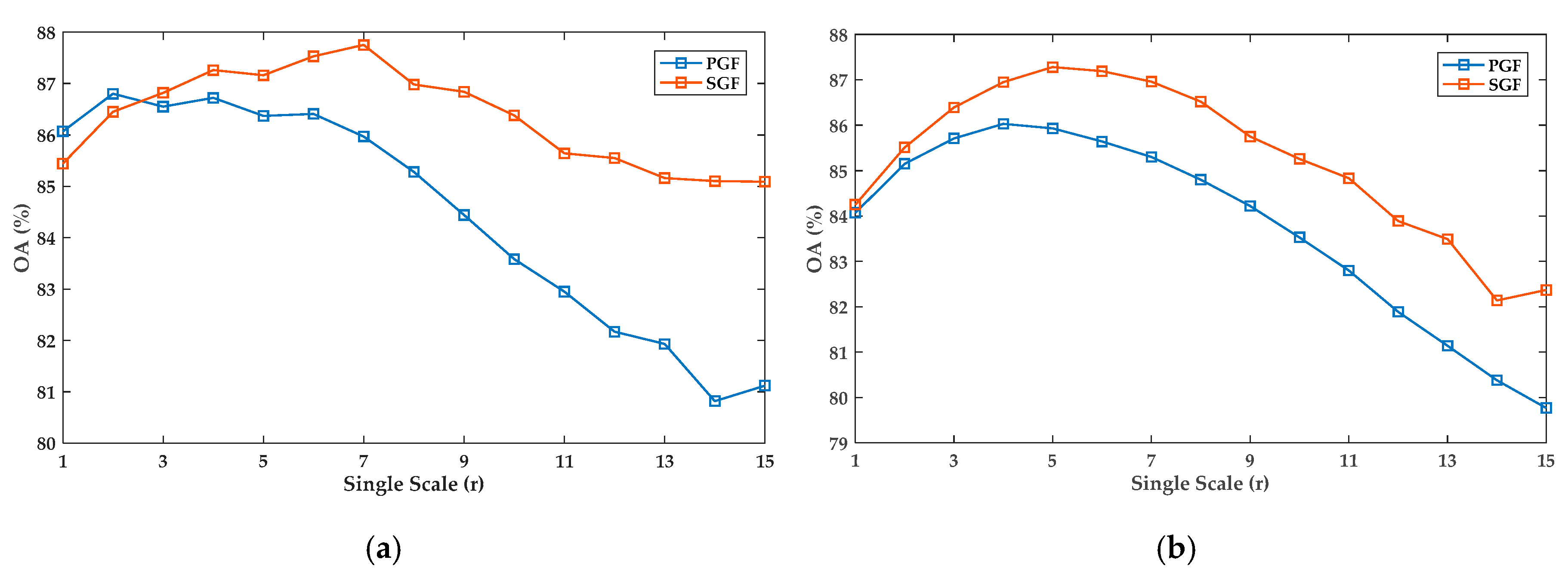
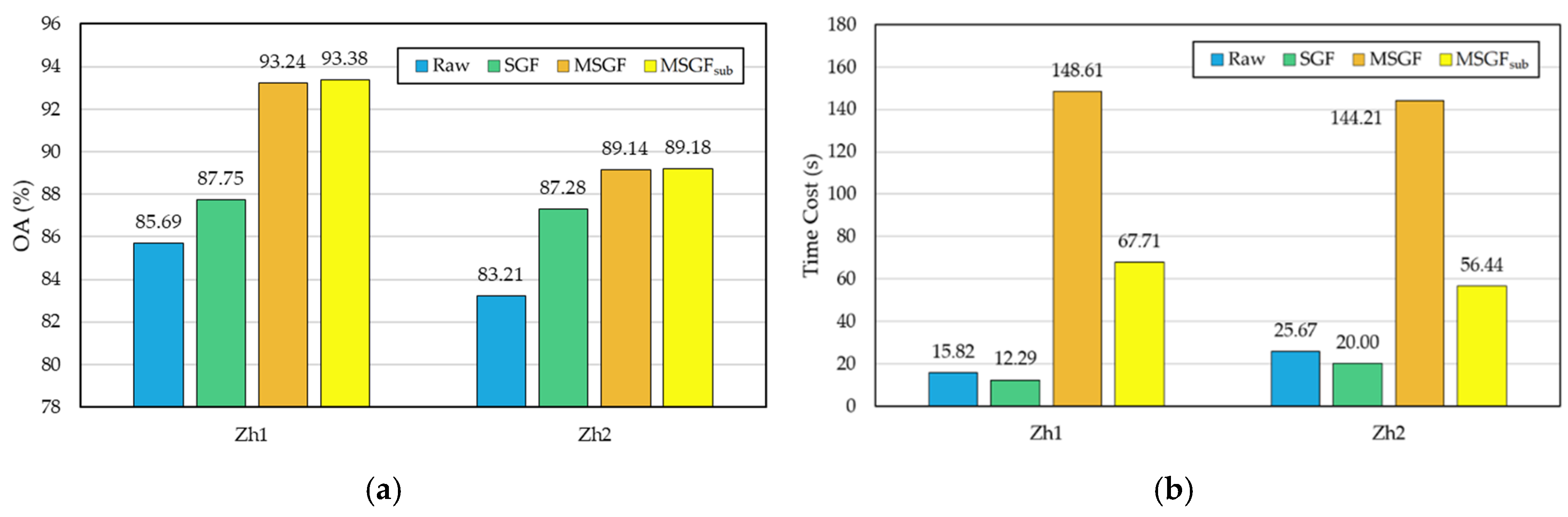
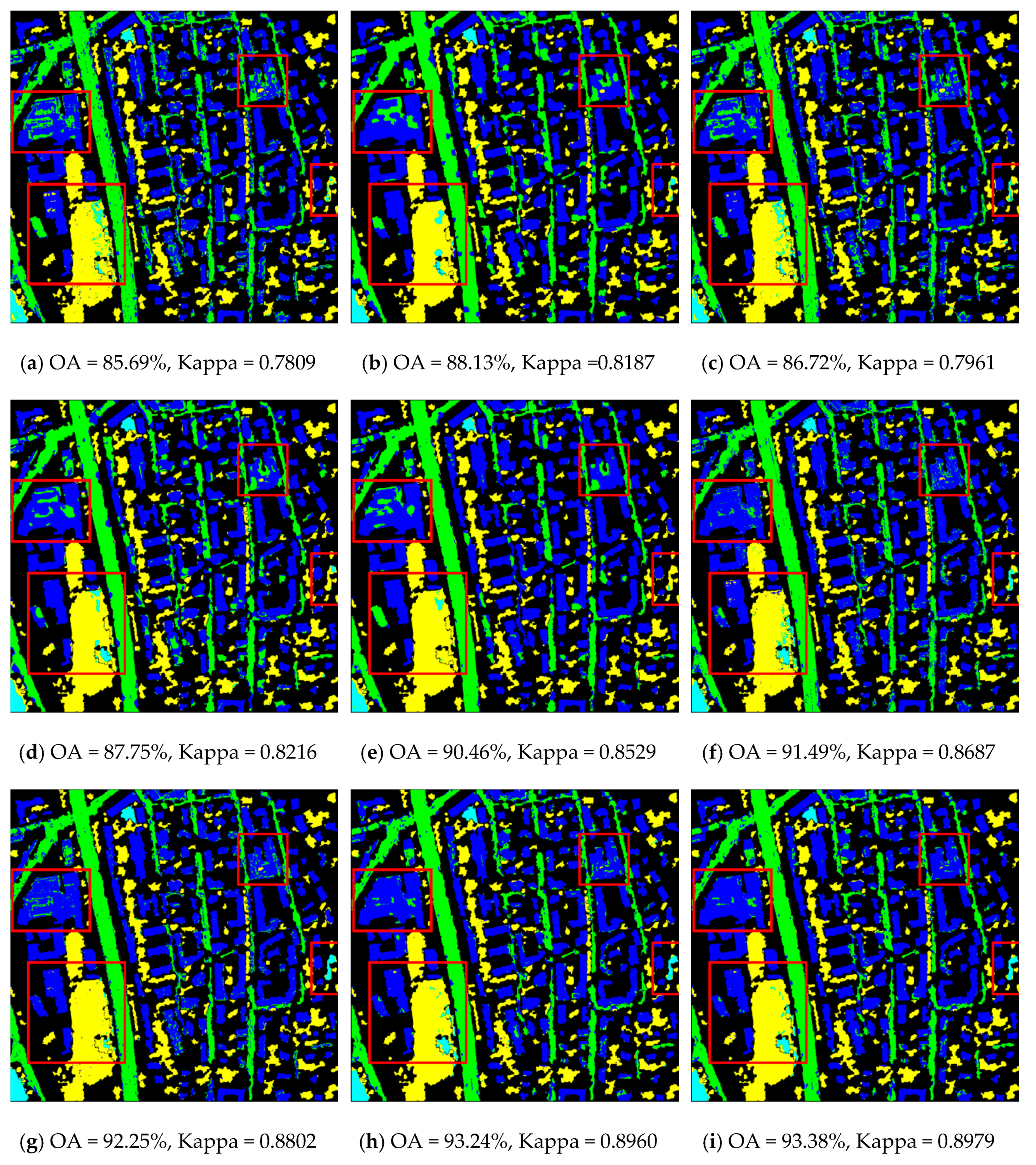
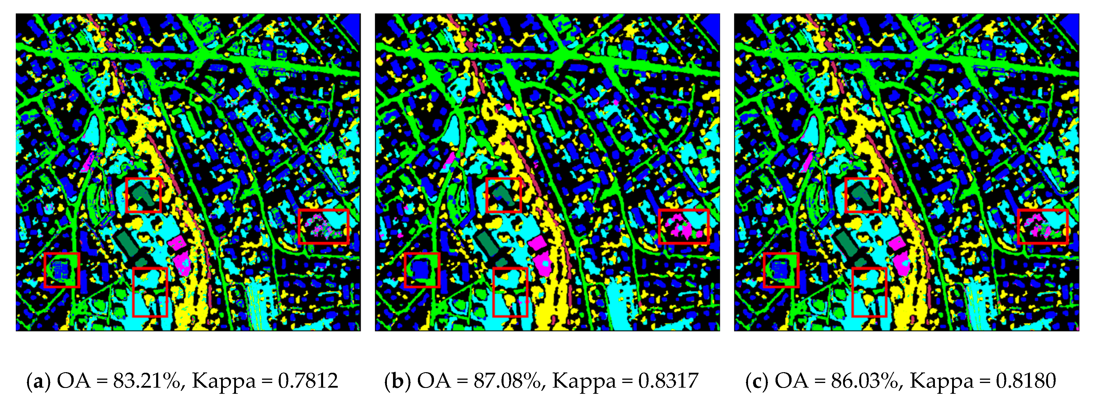
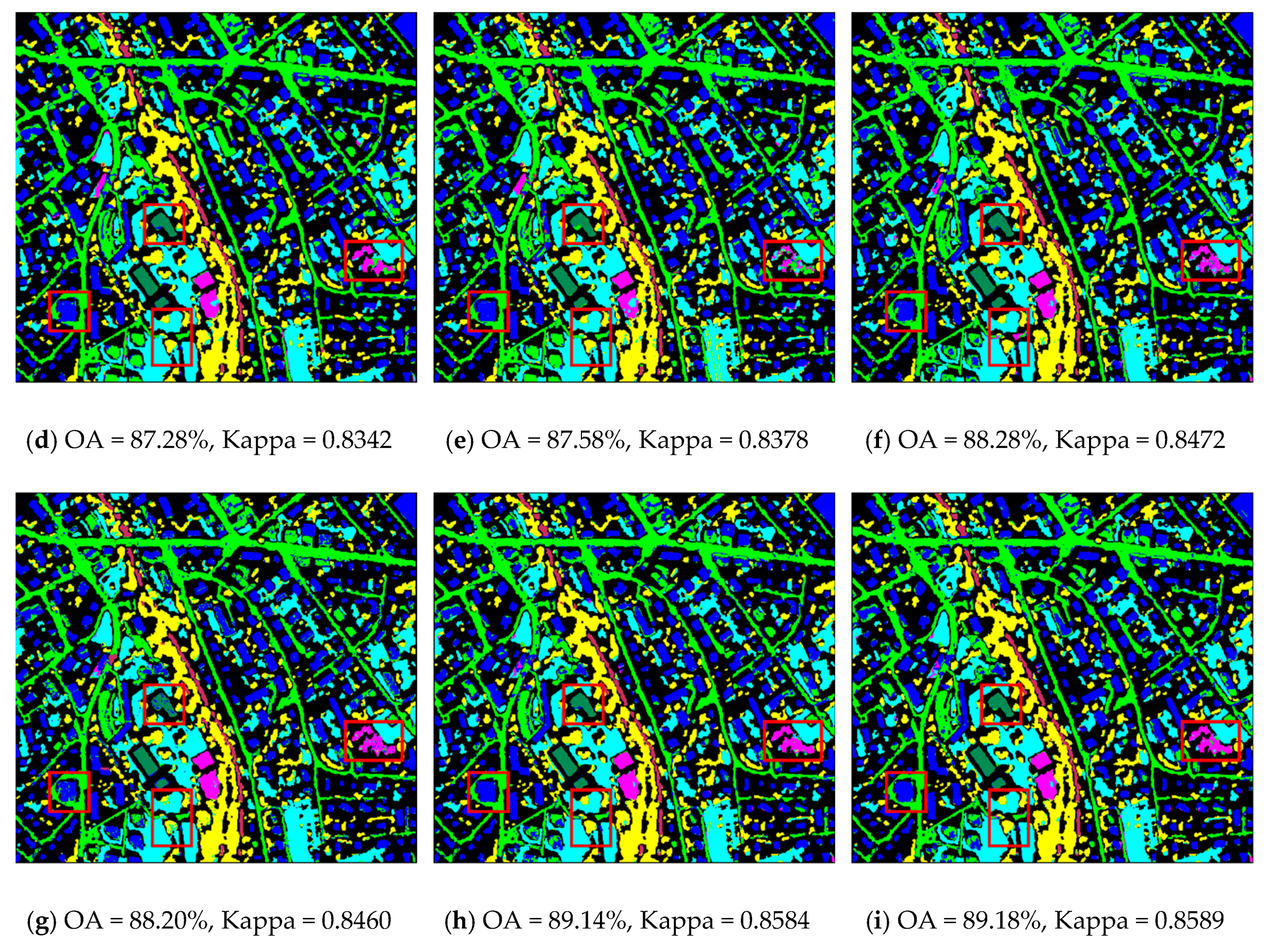
3.2.1. Results of the MSGF

By visual comparison of the features extracted by the pixel-level guided filter (PGF) and SGF (both with the scale of r = 6) in Zh1 (as shown in Figure 7), we can find that the spectral-spatial information was better preserved in the SGF feature (Figure 7b) than that of PGF (Figure 7a). Figure 8 shows the comparison of the classification accuracies obtained on PGF and SGF features at single scales on two datasets. In the experiment of Zh1, one can see that in Figure 8a, the proposed SGF outperformed the original PGF with overall higher OA values, where the highest OA value was equal to 87.75% when r = 7 and 86.80% when r = 2 in two compared approaches, respectively. Moreover, by increasing r, the accuracy of the PGF decreased more significantly, whereas the proposed SGF achieved a gentler descending trend. This confirmed the effectiveness of the proposed superpixel-based approach, which generated single-level features having better representative potential for the complex image objects. Experimental results obtained on Zh2 (as shown in Figure 8b) also indicated the effectiveness of the superpixel-level guidance image. The highest OA obtained by SGF was 87.28% when r = 5, which was higher than the one obtained by PGF with an increase of OA equal to 1.25%.
Results of both two datasets acquired by the multi-scale version of pixel-wise MPGF and the proposed MSGF were also compared. As illustrated in Figure 9, the orange curve was almost always higher than the blue curve, which indicated that at multiple stacked scales, the proposed MSGF approach outperformed the MPGF approach with significant improvement on the overall accuracy. Moreover, classification performances greatly improved with the increasing of the stacked multiple scales. For Zh1 (see Figure 9a), OA values dramatically increased to 91.98% (4.96% increased from 87.02%) in MPGF and to 93.24% (6.29% increased from 86.95%) in the proposed MSGF technique, respectively. Being similar to the first experiment, both OA values in MPGF and the proposed MSGF techniques (see Figure 9b) improved dramatically from 85.65% to 88.28% and from 85.70% to 89.14% in the experiment of the second dataset.

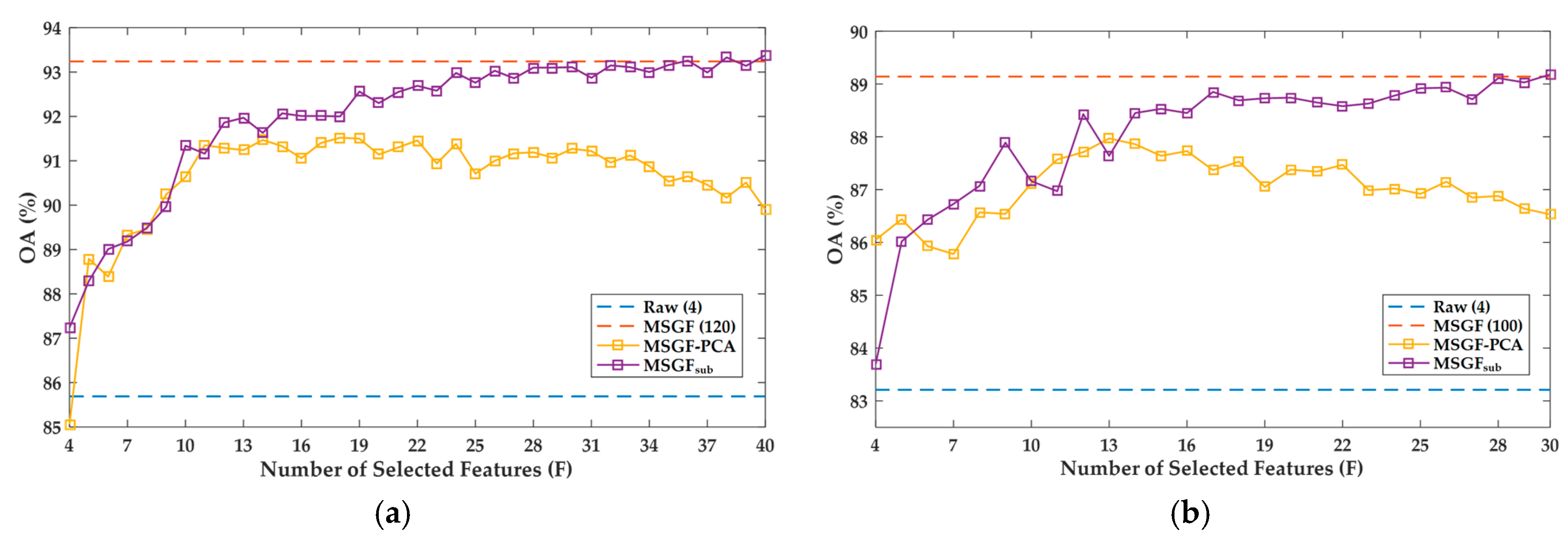
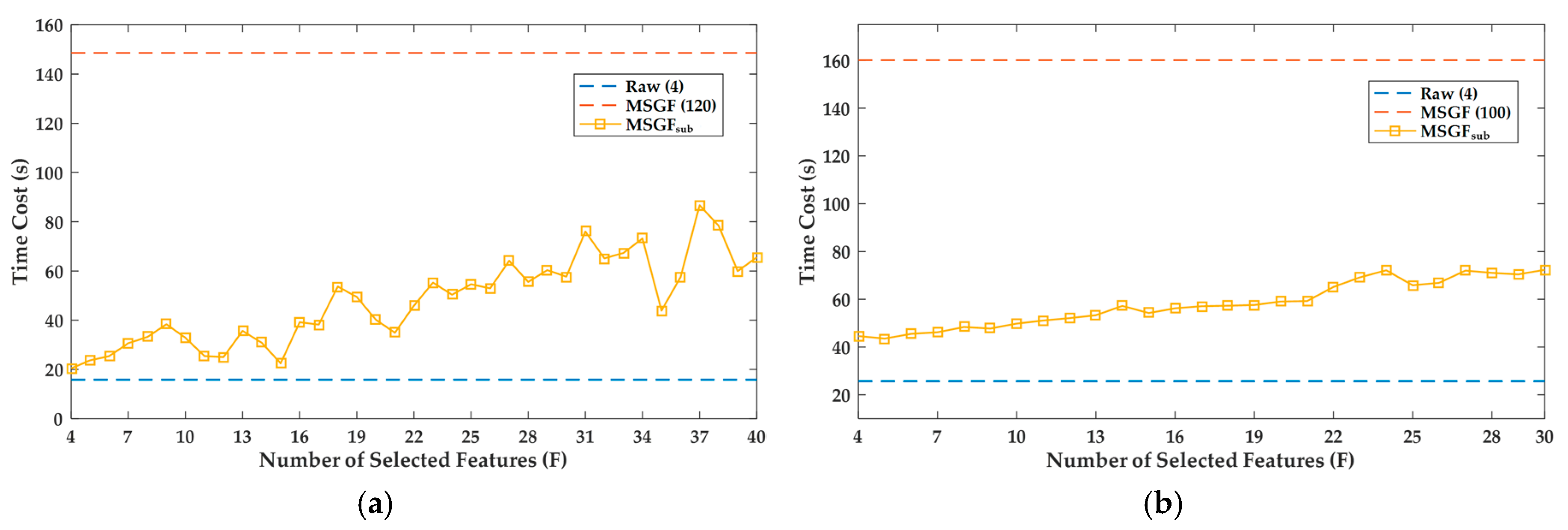
3.2.2. Role of the Feature Selection

The constructed R2 correlation matrixes based on MSGF features in the two considered datasets are illustrated in Figure 10a,b. It was clear that the blocks of those continuous bands were correlated and highly similar to each other. This meant information redundancy in the features extracted by one original band filtered with different scales.
Figure 11 is the quantitative comparison of classification results combined with and without the feature selection method. One can see that by increasing the selected number of features F, the classification performance gradually improved with the increase of OA values. In both datasets, OA values were finally close to and even exceeded the baseline. This meant that only a small feature subset could still well represent the sufficient information of the whole feature set. Furthermore, we compared the result based on feature selection with the result based on a classic feature transformation method (i.e., PCA). The results indicated that the LP algorithm presented a more stable performance superior to PCA in the classification with a reduced feature space.
The evaluation of computational efficiency in two datasets is shown in Figure 12. It can be seen that with the increasing of F, although the time consumed increased, it was still much lower than the baseline results by using the original feature set.

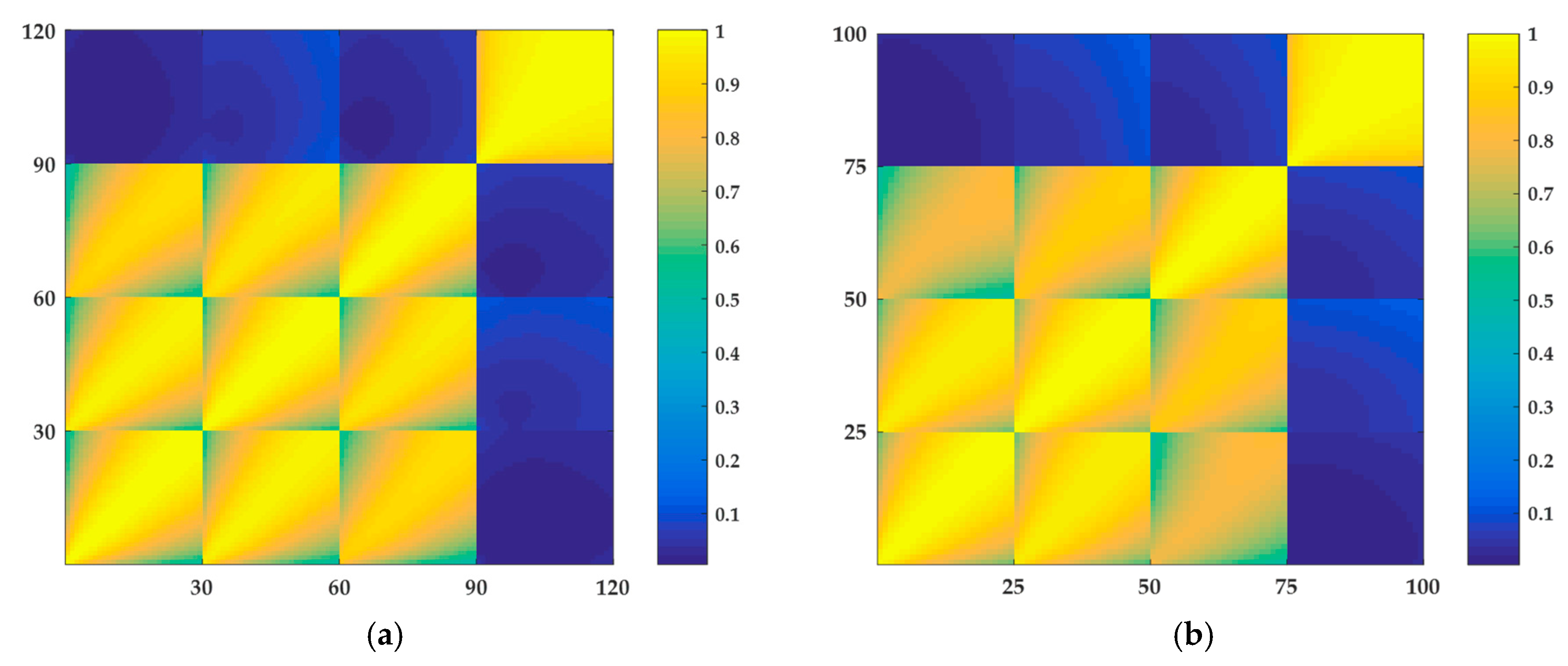
3.2.3. Component Analysis

In this subsection, additional statistics were done by combining each step of the proposed FS-MSGF method. Four classification results were compared based on (1) the raw image, (2) features extracted under the single scale (i.e., SGF), (3) multi-scale stacked features (i.e., MSGF), and (4) the proposed FS-MSGF. Figure 13 is the analysis of OA values and the time efficiency of each step. Note that the analysis was based on the result of SGF and MSGFsub. It is easy to find that in Figure 13a, each step in the proposed method had a positive influence on the final classification output. As one can see from Figure 13b, the time consumption increased dramatically with the step of high-dimensional multi-scale feature stacking and obviously decreased through the process of feature selection.

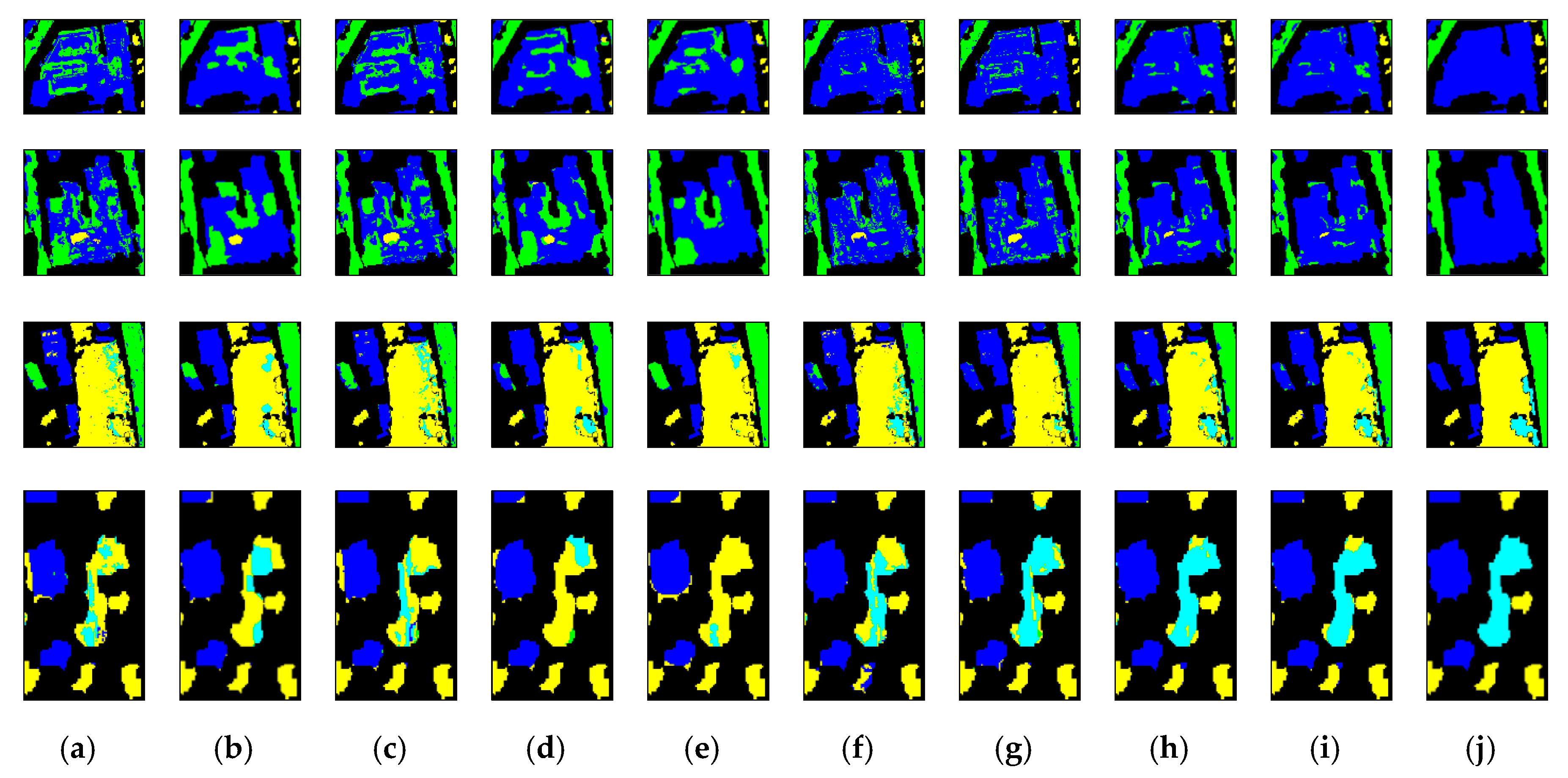
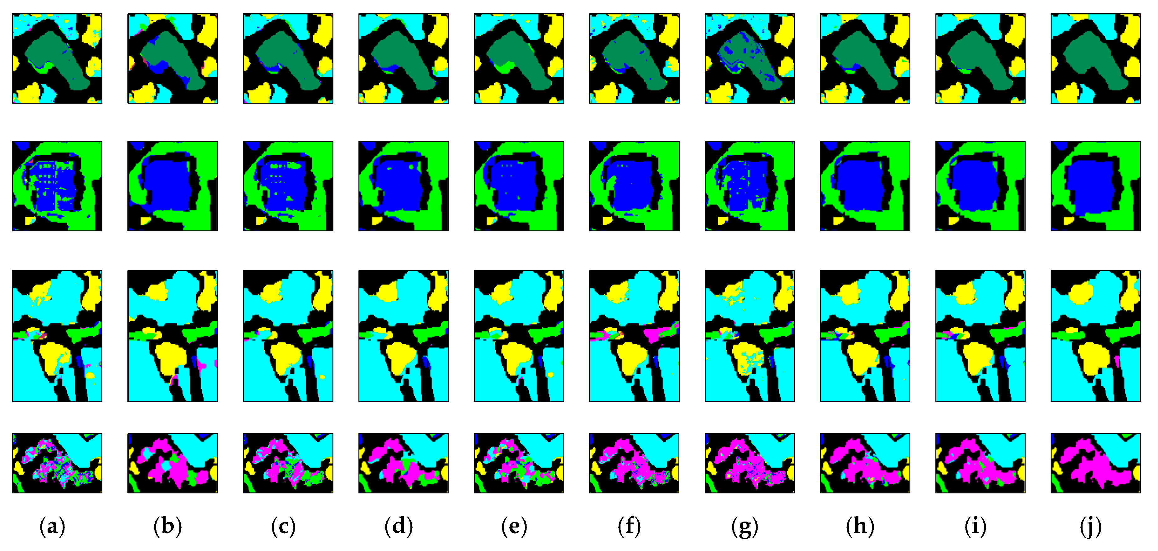
3.3. Results Comparison with Different State-of-the-Art Approaches

Furthermore, the quantitative evaluation was carried out by comparing the classification maps achieved by the proposed FS-MSGF approach with those baseline classification results including by using the original bands, the SLIC segmented original bands (SLICRaw), and also the ones obtained by several popular approaches including (1) GF-based probabilities (GFProb) [31], PGF, and SGF at single scales; and (2) the extended morphological profiles (EMPs) [35], multi-scale pixel-guided filter (MPGF) [32], and multi-scale superpixel-guided filter (MSGF) at multiple scales. It is important to note that all the reference single-scale methods were presented and compared when optimal scales were reached in each method. For multi-scale reference methods, the same stacked scales (i.e., r = [1,30] for Zh1 and r = [1,25] for Zh2) were defined to generate the results.
In the experiment of Zh1, the obtained classification maps are shown in Figure 14. As we can see from both the global and local scales (see the red boxes in Figure 14), the proposed methods (see Figure 14h,i) presented better classification result than the referenced methods (see Figure 14a–g). The quantitative analysis results with accuracies are provided in Table 2. It illustrates that the proposed multi-scale FS-MSGF approach significantly improved the baseline results at single scales (i.e., original bands and SLICRaw) according to the increase of overall accuracies (i.e., from 85.69%, to 88.13%, to 93.38%) and the Kappa coefficient (Kappa) (i.e., from 0.7809, to 0.8187, to 0.8960). The proposed FS-MSGF method resulted in better performance than the single-scale state-of-the-art (SOA) approaches (i.e., PGF, SGF, and GFProb by increasing 6.66%, 5.59%, and 2.92% in OA values, respectively). Simultaneously, the proposed method achieved similar or even better classification performance with the multi-scale methods for comparison, while it saved nearly two-thirds of the time (i.e., MPGF, EMPs, and MSGF by decreasing 60.63%, 61.18%, and 53.56% of the total time cost, respectively), which showed potential capabilities in practical applications.
Figure 15 shows the comparison between different classification results obtained on Zh2. The proposed approach (see Figure 15h,i) also resulted in a better classification performance than other methods (see Figure 15a–g), both globally and locally, especially the close-up figures below the whole classification maps. Classification accuracies are listed in Table 3. We can observe that the two proposed MSGF approaches significantly increased the single-scale baseline results with respect to the OA values (from 83.21% and 87.08% to 89.14% and 89.18%) and Kappa (from 0.7812 and 0.8317 to 0.8584 and 0.8589). FS-MSGF performed better than the single-scale SOA methods (i.e., PGF, SGF, and GFProb) by increasing the OA values to 3.15%, 1.90%, and 1.60%, respectively. Similar performance and computational cost improvements could be also found in this experiment (i.e., MPGF, EMPs, and MSGF by decreasing the time cost by 58.92%, 72.47%, and 54.82%, respectively), which further demonstrated the efficiency of the proposed techniques.

4. Discussion

The performance evaluation of the proposed approach itself and its comparison with different methods demonstrated the effectiveness of the proposed FS-MSGF in terms of high classification accuracy indices and less computational cost. In this section, we further analyze the experimental results obtained on the local scales to show the superiority of the proposed approach, especially for those land-cover classes whose gradient magnitudes were not clear. In addition, discussions and suggestions are also provided for using the FS-MSGF in practical applications.
Subsets that highlighted the whole obtained classification maps (see the red rectangular regions in Figure 14 and Figure 15) are extracted and further compared in Figure 16 and Figure 17, respectively. In general, comparing with the reference map (Column j), it was clear that the proposed MSGF and FS-MSGF (Columns h and i) outperformed all other methods (Columns a–g). The resulting land-cover classes were more inner-homogenous and spatially regular, whereas either in the baseline results or in the SOA methods, more false alarms were produced, which were mainly wrongly classified pixels inside of a local region. The results of the proposed MSGF and FS-MSGF approaches were similar (this could be also confirmed from their accuracies), but note that from the efficiency point of view, FS-MSGF could save more than half of the computational time cost. Moreover, we can also observe that the multi-scale-based approaches (Columns f–i) achieved better results than single-scale-based ones (Columns c–e). This shows that the overall classification performance could be enhanced by taking advantage of the object multi-scale information in VHR images, whereas the single-scale modelling may lead to more false alarms.
In addition, for those land-cover classes whose gradient magnitudes were not clear, the proposed MSGF and FS-MSGF approaches identified their class boundaries and shapes better than other methods. This can be observed from the local results as shown in Figure 16 Row 3 and Row 4, and also in Figure 17 Row 1 and Row 3. The grass and trees classes were very similar from the spectral point of view; however, in the proposed approaches, these two classes were successfully classified with their class boundaries and superior to all other compared methods.
In practical applications, the proposed method showed its strong potential in VHR remote sensing image classification due to its high classification accuracy and high cost efficiency. The success in using the approach depended on the good superpixel guidance information and the multi-scale information extraction. At this stage of study, we considered the proposed method to have an overall high performance based on all classes, and its accuracy might be further improved when modifying it into a class-specific version, where the multi-scale features are constructed by using GF.

5. Conclusions

We presented a novel feature selection-based multi-scale superpixel-guided filter (FS-MSGF) approach for addressing the classification task in VHR remotely sensed imagery in this work. Experiments were implemented on two QuickBird VHR datasets over the complex Zurich urban scene. From the obtained experimental results and with both qualitative and quantitative analysis, we could conclude the following:
  • Instead of using the original pixel-level guidance image, the idea of using superpixel-level guidance image significantly improved the classification performance. More accurate boundaries and homogenous context information of local objects were well preserved in the extracted multi-scale GF features.
  • Compared with the single-scale GF feature, use of multi-scale stacked features helped to model the image objects better spatially from the viewpoint of different scales. Note that such generated features could increase the land-cover class discriminability, but in the meantime, would inevitably lead to the increasing of feature dimensionality.
  • The feature subset generated by a certain feature selection technique maintained the classification performance at a high level while only using a portion of the original features. This could effectively reduce the overall computational cost without losing the overall accuracy, which is very valuable in practical applications.
This work proposed a solution for the challenging VHR image classification problem over a complex urban scene. It utilized abundant scale information of the geospatial objects in a reduced feature space, which was able to reduce the computational cost without losing the representative and refined feature in the process of classification. It also showed potential applicability for solving other similar challenging classification problems in very-high-resolution hyperspectral or thermal images.

Author Contributions

S.L. and Q.H. contributed equally to this work. Conceptualization, S.L.; methodology, Q.H. and S.L.; validation, Q.H. and X.M.; formal analysis, S.L.; investigation, X.T.; writing, original draft preparation, Q.H.; writing, review and editing, S.L., X.T., J.X. and Q.D.; visualization, A.S.; supervision, S.L.; funding acquisition, Q.D. and S.L. All authors have read and agreed to the published version of the manuscript.

Funding

This research was funded in part by National Key R&D Program of China (Grant Number 2018YFB0505000), partly by the National Natural Science Foundation of China (Grant Numbers 41601354 and 41601440), and by the Fundamental Research Funds for the Central Universities.

Acknowledgments

We would like to thank Michele Volpi from Swiss Federal Institute of Technology Zurich for providing the Zurich QuickBird VHR datasets.

Conflicts of Interest

The authors declare no conflict of interest.

References

  1. Blaschke, T.; Lang, S.; Lorup, E.; Strobl, J.; Zeil, P. Object-oriented image processing in an integrated GIS/remote sensing environment and perspectives for environmental applications. Environ. Inf. Plan. Polit. Public Metrop. Verlag Marburg 2000, 2, 555–570. [Google Scholar]
  2. Han, X.; Huang, X.; Li, J.; Li, Y.; Yang, M.Y.; Gong, J. The edge-preservation multi-classifier relearning framework for the classification of high-resolution remotely sensed imagery. ISPRS J. Photogramm. Remote Sens. 2018, 138, 57–73. [Google Scholar] [CrossRef]
  3. Alshehhi, R.; Marpu, P.R.; Woon, W.L.; Dalla Mura, M. Simultaneous extraction of roads and buildings in remote sensing imagery with convolutional neural networks. ISPRS J. Photogramm. Remote Sens. 2017, 130, 139–149. [Google Scholar] [CrossRef]
  4. Tarabalka, Y.; Chanussot, J.; Benediktsson, J.A. Segmentation and classification of hyperspectral images using watershed transformation. Pattern Recognit. 2010, 43, 2367–2379. [Google Scholar] [CrossRef] [Green Version]
  5. Csillik, O. Fast segmentation and classification of very high resolution remote sensing data using SLIC superpixels. Remote Sens. 2017, 9, 243. [Google Scholar] [CrossRef] [Green Version]
  6. Blaschke, T. Object based image analysis for remote sensing. ISPRS J. Photogramm. Remote Sens. 2010, 65, 2–16. [Google Scholar] [CrossRef] [Green Version]
  7. Zhongwen, H.; Qian, Z.; Qin, Z.; Qingquan, L.; Guofeng, W. Stepwise evolution analysis of the region-merging segmentation for scale parameterization. IEEE J. Sel. Top. Appl. Earth Obs. Remote Sens. 2018, 11, 2461–2472. [Google Scholar]
  8. Ming, D.; Li, J.; Wang, J.; Zhang, M. Scale parameter selection by spatial statistics for GeOBIA: Using mean-shift based multi-scale segmentation as an example. ISPRS J. Photogramm. Remote Sens. 2015, 106, 28–41. [Google Scholar] [CrossRef]
  9. Drǎguţ, L.; Tiede, D.; Levick, S.R. ESP: A tool to estimate scale parameter for multiresolution image segmentation of remotely sensed data. Int. J. Geogr. Inf. Sci. 2010, 24, 859–871. [Google Scholar] [CrossRef]
  10. Kuffer, M.; Pfeffer, K.; Sliuzas, R.; Baud, I. Extraction of slum areas from VHR imagery using GLCM variance. IEEE J. Sel. Top. Appl. Earth Obs. Remote Sens. 2016, 9, 1830–1840. [Google Scholar] [CrossRef]
  11. Chen, Y.; Lv, Z.; Huang, B.; Jia, Y. Delineation of built-up areas from very high-resolution satellite imagery using multi-scale textures and spatial dependence. Remote Sens. 2018, 10, 1596. [Google Scholar] [CrossRef] [Green Version]
  12. Bellens, R.; Gautama, S.; Martinez-Fonte, L.; Philips, W.; Chan, J.C.-W.; Canters, F. Improved classification of VHR images of urban areas using directional morphological profiles. IEEE Trans. Geosci. Remote Sens. 2008, 46, 2803–2813. [Google Scholar] [CrossRef]
  13. Samat, A.; Persello, C.; Liu, S.; Li, E.; Miao, Z.; Abuduwaili, J. Classification of VHR multispectral images using extratrees and maximally stable extremal region-guided morphological profile. IEEE J. Sel. Top. Appl. Earth Obs. Remote Sens. 2018, 11, 3179–3195. [Google Scholar] [CrossRef]
  14. Benediktsson, J.A.; Pesaresi, M.; Arnason, K. Classification and feature extraction for remote sensing images from urban areas based on morphological transformations. IEEE Trans. Geosci. Remote Sens. 2003, 41, 1940–1949. [Google Scholar] [CrossRef] [Green Version]
  15. Liao, W.; Dalla Mura, M.; Chanussot, J.; Bellens, R.; Philips, W. Morphological attribute profiles with partial reconstruction. IEEE Trans. Geosci. Remote Sens. 2016, 54, 1738–1756. [Google Scholar] [CrossRef]
  16. Liao, W.; Chanussot, J.; Dalla Mura, M.; Huang, X.; Bellens, R.; Gautama, S.; Philips, W. Taking optimal advantage of fine spatial resolution: Promoting partial image reconstruction for the morphological analysis of very-high-resolution images. IEEE Geosci. Remote Sens. Mag. 2017, 5, 8–28. [Google Scholar] [CrossRef] [Green Version]
  17. Samat, A.; Du, P.; Liu, S.; Li, J.; Cheng, L. E2LM: Ensemble extreme learning machines for hyperspectral image classification. IEEE J. Sel. Top. Appl. Earth Obs. Remote Sens. 2014, 7, 1060–1069. [Google Scholar] [CrossRef]
  18. Jing, W.; Chein, I.C. Independent component analysis-based dimensionality reduction with applications in hyperspectral image analysis. IEEE Trans. Geosci. Remote Sens. 2006, 44, 1586–1600. [Google Scholar] [CrossRef]
  19. Du, P.J.; Liu, S.C.; Bruzzone, L.; Bovolo, F. Target-driven change detection based on data transformation and similarity measures. In Proceedings of the 2012 IEEE International Geoscience and Remote Sensing Symposium, Munich, Germany, 22–27 July 2012; pp. 2016–2019. [Google Scholar]
  20. De Backer, S.; Kempeneers, P.; Debruyn, W.; Scheunders, P. A band selection technique for spectral classification. IEEE Geosci. Remote Sens. Lett. 2005, 2, 319–323. [Google Scholar] [CrossRef]
  21. Ifarraguerri, A.; Prairie, M.W. Visual method for spectral band selection. IEEE Geosci. Remote Sens. Lett. 2004, 1, 101–106. [Google Scholar] [CrossRef]
  22. Huang, R.; He, M. Band selection based on feature weighting for classification of hyperspectral data. IEEE Geosci. Remote Sens. Lett. 2005, 2, 156–159. [Google Scholar] [CrossRef]
  23. Du, Q.; Yang, H. Similarity-based unsupervised band selection for hyperspectral image analysis. IEEE Geosci. Remote Sens. Lett. 2008, 5, 564–568. [Google Scholar] [CrossRef]
  24. Jia, S.; Tang, G.; Zhu, J.; Li, Q. A novel ranking-based clustering approach for hyperspectral band selection. IEEE Trans. Geosci. Remote Sens. 2015, 54, 88–102. [Google Scholar] [CrossRef]
  25. Tschannerl, J.; Ren, J.; Yuen, P.; Sun, G.; Zhao, H.; Yang, Z.; Wang, Z.; Marshall, S. MIMR-DGSA: Unsupervised hyperspectral band selection based on information theory and a modified discrete gravitational search algorithm. Inf. Fusion 2019, 51, 189–200. [Google Scholar] [CrossRef] [Green Version]
  26. Li, S.; Kang, X.; Hu, J. Image fusion with guided filtering. IEEE Trans. Image Process. 2013, 22, 2864–2875. [Google Scholar]
  27. Zhang, Q.; Li, X.R. Fast image dehazing using guided filter. In Proceedings of the 2015 IEEE 16th International Conference on Communication Technology (ICCT), Hangzhou, China, 18–20 October 2015; pp. 182–185. [Google Scholar]
  28. Guo, L.; Chen, L.; Chen, C.P.; Zhou, J. Integrating guided filter into fuzzy clustering for noisy image segmentation. Digit. Signal Process. 2018, 83, 235–248. [Google Scholar] [CrossRef]
  29. Wang, C.; Fan, Y.Y. Saliency detection using iterative dynamic guided filtering. In Proceedings of the 24th International Conference on Pattern Recognition (ICPR), Beijing, China, 20–24 August 2018; pp. 3396–3401. [Google Scholar]
  30. He, K.; Sun, J.; Tang, X. Guided image filtering. IEEE Trans. Pattern Anal. Mach. Intell. 2012, 35, 1397–1409. [Google Scholar] [CrossRef]
  31. Kang, X.; Li, S.; Benediktsson, J.A. Spectral–spatial hyperspectral image classification with edge-preserving filtering. IEEE Trans. Geosci. Remote Sens. 2013, 52, 2666–2677. [Google Scholar] [CrossRef]
  32. Wang, L.; Cao, X.; Zheng, Y.; Dai, Q. Multi-scale feature extraction of hyperspectral image with guided filering. J. Remote Sens. 2018, 22, 293–303. [Google Scholar]
  33. Achanta, R.; Shaji, A.; Smith, K.; Lucchi, A.; Fua, P.; Süsstrunk, S. SLIC superpixels compared to state-of-the-art superpixel methods. IEEE Trans. Pattern Anal. Mach. Intell. 2012, 34, 2274–2282. [Google Scholar] [CrossRef] [Green Version]
  34. Heinz, D.C. Fully constrained least squares linear spectral mixture analysis method for material quantification in hyperspectral imagery. IEEE Trans. Geosci. Remote Sens. 2001, 39, 529–545. [Google Scholar] [CrossRef] [Green Version]
  35. Benediktsson, J.A.; Palmason, J.A.; Sveinsson, J.R. Classification of hyperspectral data from urban areas based on extended morphological profiles. IEEE Trans. Geosci. Remote Sens. 2005, 43, 480–491. [Google Scholar] [CrossRef]
Figure 1. Zurich Dataset 1: (a) color-infrared composite (R: band 4; G: band 3; B: band 2) of the QuickBird imagery and (b) its reference map.
Remotesensing 12 00862 g001
Figure 2. Zh2: (a) color-infrared composite (R: band 4; G: band 3; B: band 2) of the QuickBird imagery and (b) its reference map.
Remotesensing 12 00862 g002
Figure 3. Block scheme of the proposed feature selection-based multi-scale superpixel guided filter (FS-MSGF) method for classification of the VHR remotely sensed imagery. LP, linear prediction.
Remotesensing 12 00862 g003
Figure 4. An example of the guided filtered result based on the QuickBird images: (a) input image I; (b) the guidance image G; 3D comparison of band features: (c) before and (d) after GF.
Remotesensing 12 00862 g004
Figure 5. The segmentation result in (a) and guidance images for comparison purposes: (b) in the original pixel-based GF and (c) in the proposed superpixel-based GF (Zh1).
Remotesensing 12 00862 g005
Figure 6. The segmentation result in (a) and guidance images for comparison purposes: (b) in the original pixel-based GF and (c) in the proposed superpixel-based GF (Zh2).
Remotesensing 12 00862 g006
Figure 7. Visual comparison (Bands: 4, 3, 2) of: (a) pixel-level guided filter (PGF) features and (b) SGF features with the scale of r = 6.
Remotesensing 12 00862 g007
Figure 8. Single-scale classification performance comparison between the proposed SGF and the original PGF approaches obtained on: (a) Zh1 and (b) Zh2.
Remotesensing 12 00862 g008
Figure 9. Performance comparison for multiple scales’ classification between the proposed MSGF and the reference MPGF techniques obtained on: (a) Zh1 and (b) Zh2.
Remotesensing 12 00862 g009
Figure 10. The R2 correlation matrixes of MSGF features generated on: (a) Zh1; and (b) Zh2.
Remotesensing 12 00862 g010
Figure 11. Comparison of the classification accuracy with feature selection and without feature selection: (a) results on Zh1 and (b) results on Zh2.
Remotesensing 12 00862 g011
Figure 12. Comparison of the time efficiency with feature selection and without feature selection: (a) results on Zh1 and (b) results on Zh2.
Remotesensing 12 00862 g012
Figure 13. Analysis of the impact of different steps in the proposed FS-MSGF method on: (a) OA values and (b) computational efficiency.
Remotesensing 12 00862 g013
Figure 14. Classification maps obtained by: (a) original bands; (b) SLICRaw (when S = 15); (c) PGF (with r = 2); (d) SGF (with r = 7); (e) GFProb (with r = 14); (f) MPGF (with r = [1,30]); (g) extended morphological profiles (EMPs) (with r = [1,30]); (h) the proposed MSGF (with r = [1,30]); (i) the proposed FS-MSGF (with r = [1,30] and F = 40) (Zh1).
Remotesensing 12 00862 g014
Figure 15. Classification maps (and the close-up figures in the red boxes) obtained by: (a) original bands; (b) SLICRaw (when S = 15); (c) PGF (with r = 4); (d) SGF (with r = 5); (e) GFProb (with r = 6); (f) MPGF (with r = [1,25]); (g) EMPs (with r = [1,25]); (h) the proposed MSGF (with r = [1,25]); (i) the proposed FS-MSGF (with r = [1,25] and F = 30) (Zh2).
Remotesensing 12 00862 g015aRemotesensing 12 00862 g015b
Figure 16. Comparison of local classification results obtained by: (a) original bands; (b) SLICRaw (when S = 15); (c) PGF (with r = 2); (d) SGF (with r = 7); (e) GFProb (with r = 14); (f) MPGF (with r = [1,30]); (g) EMPs (with r = [1,30]); (h) the proposed MSGF (with r = [1,30]); (i) the proposed FS-MSGF (with r = [1,30] and F = 40); (j) the reference map, where the four rows correspond to the four sub-regions highlighted in Figure 14 (Zh1).
Remotesensing 12 00862 g016
Figure 17. Comparison of local classification results obtained by: (a) original bands; (b) SLICRaw (when S = 15); (c) PGF (with r = 4); (d) SGF (with r = 5); (e) GFProb (with r = 6); (f) MPGF (with r = [1,25]); (g) EMPs (with r = [1,25]); (h) the proposed MSGF (with r = [1,25]); (i) the proposed FS-MSGF (with r = [1,25] and F = 30); (j) the reference map, where four rows correspond to four sub-regions highlighted in Figure 15 (Zh2).
Remotesensing 12 00862 g017
Table 1. Detailed sample information used in the experiment (pixels).
Zh1Zh2
ClassTrainingTestClassTrainingTest
Roads86685,685Roads774154,012
Buildings1542152,622Buildings753149,874
Grass726391Grass555128,570
Trees81080,961Trees646110,426
Bare Soil5310,566
Water458995
Pools306022
Table 2. Classification results of Zh1 obtained by the proposed and reference methods.
Classification ApproachesOverall Accuracy (OA) (%)Kappa Coefficient (Kappa)Time Cost (s)
BaselineOriginal Bands85.690.780915.82
SLICRaw (when S = 15)88.130.81878.24
Single ScalePGF (with r = 2)86.720.796115.08
SGF (with r = 7)87.750.812612.29
GFProb (with r = 14)90.460.852917.72
Multiple ScalesMPGF (with r = [1,30])91.490.8687189.45
EMPs (with r = [1,30])92.250.8802192.10
proposed MSGF (with r = [1,30])93.240.8960160.59
proposed FS-MSGF (with r = [1,30] and F = 40)93.380.897974.58
Table 3. Classification results of Zh2 obtained by the proposed and reference methods.
Classification ApproachesOverall Accuracy (OA) (%)Kappa Coefficient (Kappa)Time Cost (s)
BaselineOriginal Bands83.210.781225.67
SLICRaw (when S = 15)87.080.831716.13
Single ScalePGF (with r = 4)86.030.818023.20
SGF (with r = 5)87.280.834220.00
GFProb (with r = 6)87.580.837828.62
Multiple ScalesMPGF (with r = [1,25])88.280.8472176.11
EMPs (with r = [1,25])88.200.8460262.78
Proposed MSGF (with r = [1,25])89.140.8584160.11
proposed FS-MSGF (with r = [1,25] and F = 30)89.180.858972.34

