1. Introduction
Soil moisture is a key variable that controls major physical processes in numerical weather prediction, climate simulation, crop growth models, and flood forecasting by controlling the surface energy distribution of sensible heat and latent heat fluxes in terrestrial–atmosphere coupling and energy and water cycling [
1,
2,
3,
4,
5]. Accurate observation of high precision soil moisture data is of great significance for crop growth, drought monitoring, and monitoring global climate change [
6,
7,
8,
9].
At present, soil moisture data are obtained through three main methods: (1) Simulating soil moisture using land surface process models and hydrological models [
10,
11,
12]. (2) Measuring soil moisture through ground meteorological observatories [
13]. (3) Using remote sensing data to retrieve soil moisture [
14,
15,
16,
17,
18]. Currently, optical and microwave technologies are widely used for monitoring soil moisture, which compensates for the space-time discontinuity in the site to some extent and can obtain large-scale soil moisture observation data by conducting large-scale and even global observations. However, the retrieval method is highly susceptible to the uncertainties associated with the instruments and algorithms. Moreover, the coverage of surface vegetation also greatly affects the accuracy of remote sensing retrieval. In summary, making the soil moisture data of each system complement each other and using the high-precision large-scale soil moisture data with a continuous time scale is a worthy research topic.
Land surface data assimilation technology, as a method of integrating the multi-geographic spatial data, combines new observation data in the dynamic operation of numerical models to obtain datasets with temporal, spatial, and physical heterogeneity [
19,
20]. The land surface data assimilation algorithm is mainly divided into two categories: continuous data assimilation algorithm and sequential data assimilation algorithm [
21,
22,
23,
24,
25,
26]. The ensemble Kalman filter (EnKF) algorithm proposed by Evensen in 1994 is an efficient sequential data assimilation algorithm [
27,
28]. It is based on the Monte Carlo (MC) method that obtains the background error covariance matrix in practical applications using the idea of ensemble and reduces the number of calculations, having a good effect on data assimilation when dealing with nonlinear systems. Reichle and Koster [
29] assimilated the global scale soil moisture data from the scanning multichannel microwave radiometer (SMMR) into the National Aeronautics and Space Administration (NASA) catchment land surface model (CLSM) using the EnKF, and verified them with ground-based measurements. The experimental results showed that the values obtained by data assimilation were better than those of satellite data and the model simulated data and that the data assimilation improved the estimation accuracy of soil moisture in the root zone. It proved that data assimilation could obtain better soil moisture estimation by combining the model simulation data with independent information from remote sensing observation data. Gruber et al. [
30] used the triple collocation (TC) method to obtain error covariance statistics for both the modelling and observation subcomponents of a data assimilation system and the linear antecedent precipitation index (API) model, and the soil moisture data from the ground observation sites were assimilated using a Kalman filter, to analyze the advantages of the assimilation method for existing remote sensing observation data. Renzullo et al. [
31] developed a terrestrial soil moisture data assimilation system framework for the Australian Water Resources Assessment (AWRA) modelling system. The advanced microwave scanning radiometer—earth observing system (AMSR-E) and advanced scatterometer (ASCAT) satellite soil moisture inversion data were assimilated into the AWRA-L system and compared with the soil moisture site measurements and also with a new network of cosmic-ray moisture probes (CosmOz) spread across the country. It has been demonstrated that the assimilation of AMSR-E and ASCAT soil moisture products into the AWRA-L model could improve the soil moisture estimates, especially in the root-zones layer. Kolassa et al. [
32] studied the data assimilation of soil moisture active passive (SMAP) observations, compared different methods for extracting soil moisture information, and used different methods of adjusting observations to determine the effective method to assimilate the SMAP soil moisture observations into the CLSM. The previous studies have shown that data assimilation through the inversion of soil moisture products by microwave remote sensing can improve the estimation accuracy of soil moisture.
In land surface data assimilation, it is usually assumed that the model is perfect (for example, ignoring model errors) [
33]. However, this assumption is problematic even in the application of relatively simpler models, and with more complexities in the model, the influence of model errors on the data assimilation results becomes more significant. Generally, model prediction error comes from three factors: (1) initial conditions, (2) forcing data, and (3) model equations [
34]. In the EnKF data assimilation, different research areas, different land surface models, and different forcing data will bring a large number of uncertainties to the background field error and data assimilation results. Moreover, the real distribution of the model errors is also complex and diverse. Reichle et al. [
35] used non-Gaussian errors to generate a large-scale ensemble and experimentally proved that the ‘good’ ensemble had a great influence on the background field error variance estimation of EnKF data assimilation. Turner et al. [
34] systematically generalized the error sources of three models and analyzed the error conditions of the initial conditions and forcing data among the three error factors, perturbing the initial field and forcing data to assimilate the sea surface temperature. Kai et al. [
36] and Reichle et al. [
37] used the standard distributed random number as a random error, to perturb the forcing data to generate ensembles for the EnKF model error estimation. Kumar et al. [
38] and Kumar et al. [
39] applied the standard distributed random number perturbation to forcing data, model parameters, and soil moisture initial fields to generate ensembles. As an important part of the EnKF data assimilation algorithm, the ensemble is the key to express the model error. The estimation of model error from the dispersion between each ensemble member is the advantage of using the EnKF algorithm, which is different from other data assimilation algorithms. Most of the previous studies used the classical MC method to perform error perturbation on the initial field of soil moisture or forcing data and rarely incorporated the model information into the perturbation. The MC method [
40,
41] is a purely statistical initial value perturbation method. It is usually assumed that the random error of the initial and background fields obeys the standard Gaussian distribution, but this is only an idealized assumption, not a real situation. Another disadvantage of the MC method is that the model information is not included in the perturbation field and the model error is usually not fully expressed in the initial field.
In view of the aforementioned problems, this study uses the breeding of growing modes (BGM) instead of the MC method as the main perturbation method of data assimilation for the initial field and background field, and proposes a theoretical framework of the EnKF data assimilation based on the BGM perturbation method. The BGM method is one of the main methods for generating initial perturbation in numerical prediction [
42,
43]. The method generates an initial perturbation field by multiple incubations of the model and the cycle of the perturbation error increases, increasing the proportion of the high-speed growth error continuously, thereby rapidly reaching saturation. The BGM method cultivates the perturbation field through the model, so that the perturbation field would contain the model information, which is more in line with the error distribution state under the real situation. When using the BGM method to generate the perturbation field, determining the breeding length and ensemble size are key points. To generate the perturbation field with different models, different parameters need to be set. Therefore, the BGM method is used in this study to perturb the EnKF data assimilation, and experiments are conducted to evaluate the effects of growth mode breeding length and ensemble size on the EnKF assimilation. In this paper, a theoretical framework of the EnKF data assimilation based on the BGM method is proposed for soil moisture estimation. The framework includes two components: using the BGM method to generate the initial field and the BGM method based on EnKF data assimilation. Firstly, this paper discusses the two ensemble perturbation problems, i.e., the breeding length and the ensemble size in the BGM method. For the study area, a breeding length of 72 h and an ensemble size of 100 were found to be the best solution for data assimilation. On this basis, this study evaluates the impact of the BGM method and the MC method on data assimilation in detail. The Climate Change Initiative (CCI) data and in situ data are used for validating the accuracy and quality of the soil moisture estimated by the EnKF data assimilation, based on the BGM method.
The paper is organized as follows. The theoretical background of the BGM and the EnKF is given in
Section 2. Brief introductions to the variable infiltration capacity (VIC) model, the study area, remotely sensed soil moisture products, in situ data, and data pre-processing are provided in
Section 3. Details of the experiments and discussion of the results are presented in
Section 4 and
Section 5. Finally,
Section 6 summarizes the conclusions and discusses future research directions.
2. Methodology
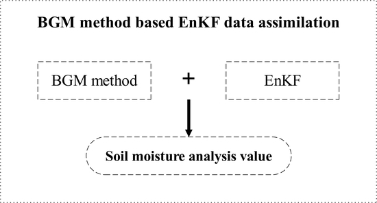
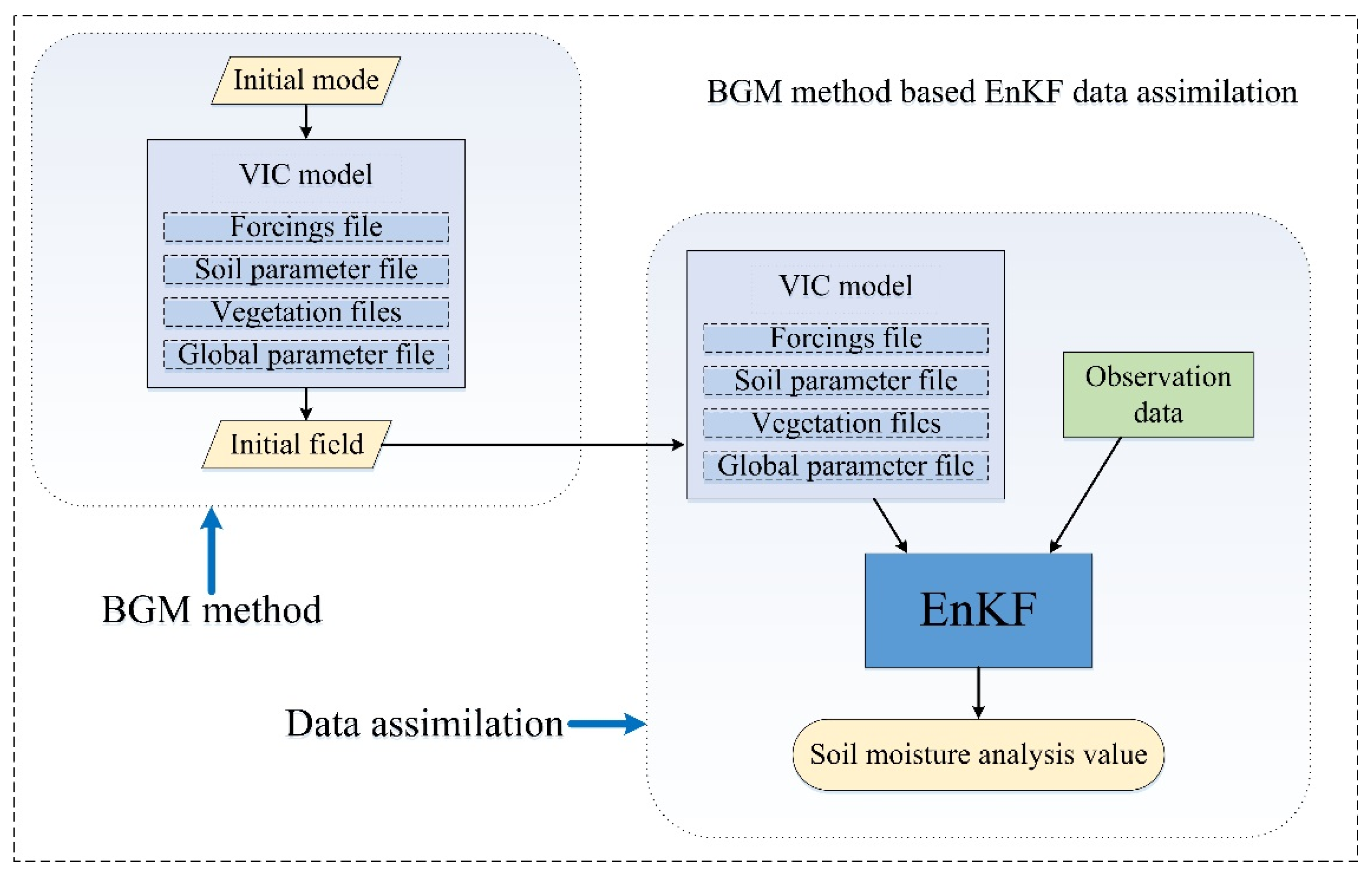
In this study, we propose an EnKF data assimilation framework based on the BGM perturbation method. The BGM method is used to generate the perturbation field to perturb the initial and background fields. The EnKF assimilation algorithm is then used to perform data assimilation to obtain the analysis value of soil moisture.
Figure 1 shows the theoretical framework of the EnKF data assimilation based on the BGM method. The perturbation principle and specific details of the BGM method are introduced in
Section 2.1. The EnKF data assimilation is described in
Section 2.2.
2.1. Breeding of Growing Modes
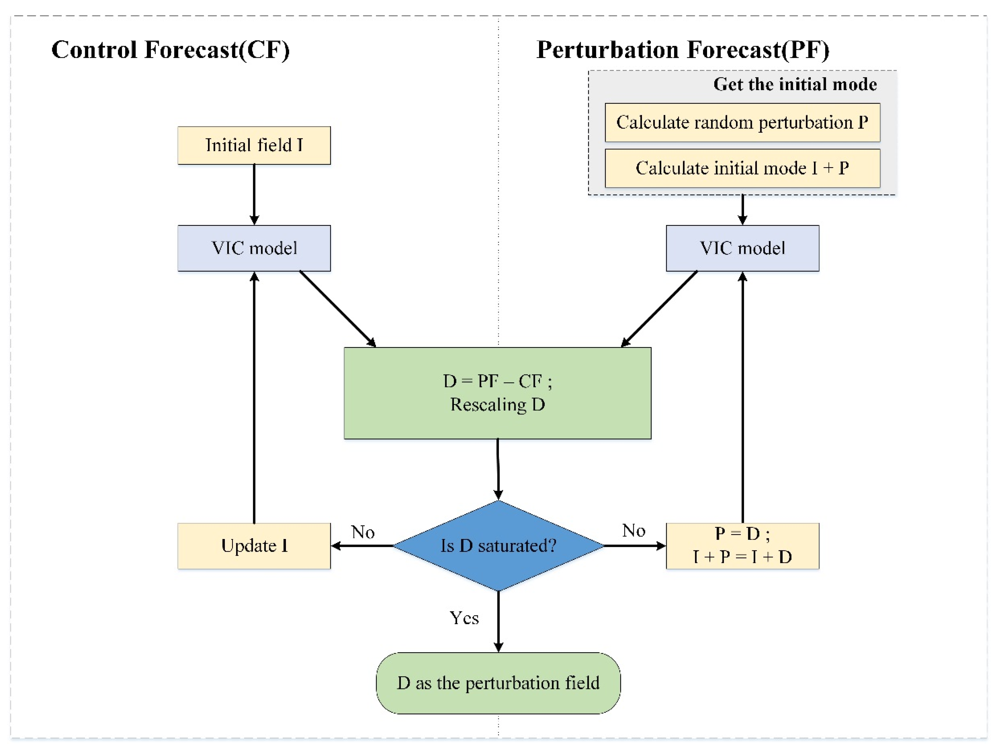
With the initial ensemble perturbations, we must provide an accurate representation of the probability distribution of the true state of the land surface. The shape of this probability distribution will depend on the kind of errors in the true state. If the likelihood of an error pattern is high, we should assign a higher probability to the true state plus or minus that particular error pattern. The BGM method is based on the notion that using the land surface model to dynamically propagate information about the state of the system in space and time will accumulate growing errors by virtue of the perturbation dynamics [
42,
43]. Compared to other initial distribution methods, this method is more advantageous because of its clear dynamic meaning, simple operation, and low computational cost. In 1992, it was commercialized at the National Centers for Environmental Prediction (NCEP).
Normally, the main sources of model forecast errors can be classified as follows: (1) initial conditions (in this paper, the initial field of soil moisture is specified. Since the true value of soil moisture under natural conditions is unknown, the initial field of soil moisture contains random errors.); (2) boundary conditions (the true value of atmospheric forcing data is also not available. In land surface models and hydrological models, the uncertainty of the forcing data will also bring great uncertainty to the model simulation.); and (3) model equations (since the model uses parameterization and the equation of natural physical processes, the model itself will also bring uncertainty to the estimation of soil moisture). In general, soil moisture estimation using ensembles can be represented by a series of numerical integrals:
where
smi(
T) represents the estimated soil moisture model at time
T;
smi(0) represents the initial field of the soil moisture; M represents the land surface model; and
f represents the atmospheric forcing data. Compared with the MC method, the BGM method uses the model integral to cultivate the perturbation field. As the cycle of the perturbation error increases, the proportion of the high-speed growth error increases continuously and later quickly reaches saturation. The BGM method is mainly divided into the following steps:
(1) First, a small random perturbation
P0 is added to the initial field
I0 of the model as the initial mode at the initial time
t0. The initial mode refers to the growth mode that has not been propagated, and its selection is the first step in implementing the growth mode breeding cycle. There are many ways to select the initial mode. In this study, the initial mode is selected using Equation (2):
where
P(
z) is the initial mode of the breeding cycle;
t is the adjustment coefficient used to control the initial mode size;
b is the Gaussian distribution random number obeying the mean of 0 variance as the model error variance Q; and
E(
z) is the root mean square error of soil moisture.
(2) Next, we integrate the original initial field I0 and the initial field perturbed by the initial mode, i.e. the perturbation field (I0 + P0), as the initial field of the model and the duration of the integration is recorded as (t1 − t0). By estimating the two soil moisture values through the model simulation, we refer to the soil moisture model estimate using the initial field I0 as the initial field of the model as the control forecast value CF and refer to the soil moisture model estimate using perturbation field I0 + P0 as the initial field of the model, as the perturbation forecast value PF.
(3) At time t1, the difference between the perturbation prediction value and the control forecast value is calculated as D1 = PF1 − CF1. To keep the D1 consistent with the magnitude of the original random perturbation P0, the size of D1 is adjusted. The resized D1 is taken as the new perturbation P1 at the next moment. (The process of readjusting the size of D1 is called ‘rescaling’).
(4) Adding the newly obtained perturbation P
1 to the model state value I
1 at the corresponding time t
1 and repeating the processes (2)–(4), we use the model to propagate the perturbation field for a period of time. After several breeding cycles, when the growth rate of the perturbation gradually stabilizes at a certain value, we obtain the ideal perturbation field. The process of the BGM method is illustrated in
Figure 2.
The BGM method simulates the development of growing errors in the model forecast cycle. Compared with the MC method, the BGM method can appropriately adjust the distribution state of the land surface to make its distribution closer to the real state. In data assimilation of the land surface, the BGM method is used to perturb the error of the initial field and the data assimilation model, to permit the physical process of the model to participate in the generation of perturbation. In this way, the perturbation contains not only the statistical information but also the physical information of the error. Compared with the singular vector (SV) method, the BGM method needs less calculation and has higher computational efficiency while attaining the same perturbation effect.
2.2. The BGM Method Based on the EnKF Data Assimilation
The basic idea of the EnKF algorithm is to perturb the state to generate a series of state ensembles, where each ensemble represents a possible value of the state, and the mean value of the ensembles is the optimal estimate of the state. The model is then used to integrate the ensemble forward and predicts the state of each ensemble at the next moment. Each ensemble is updated separately using the observation data. At this point, the mean of all ensembles is the optimal estimation value of the state and the variance of the estimated value could also be calculated through the ensemble. The EnKF algorithm includes two steps, i.e., forecast and update: (1) In the forecast stage, the ensembles of forecast fields are obtained by perturbing a single initial state variable. In this study, the BGM method is used to obtain the ensembles of perturbations. After the ensembles are acquired, the forecast error covariance matrix of the model is calculated using the forecast ensemble. (2) In the update phase, each state variable is updated using the observation value and the observation error covariance matrix, to obtain analysis field ensembles and finally, the mean value of the analysis ensemble is calculated to obtain the analysis value of the model state variable.
2.2.1. Forecast
The forecast process is calculated by the following equation:
where
xai,k-1 is the analysis value of the
i-th ensemble member at time
k-1;
xfi,k is the forecast value of the
i-th ensemble member at time
k;
Mk-1,k is a nonlinear model operator; and
wi,k-1 is the
k-1 moment model error. The model error ensemble in this study uses the perturbation field obtained by the BGM method.
2.2.2. Update
In the EnKF, noise that follows the normal distribution is added to the observations, described as follows:
where
yoi,k is the observation corresponding to the
i-th ensemble member at time
k;
vi,k is the observed error perturbation at time
k that obeys a mean of 0; and the covariance matrix is a normal distribution of
Rk. The observation error covariance matrix
Rk at time
k is:
where
Dk = [
v1,k,
v2,k,...,
vN,k],
i = 1, 2,...,
N represents the ensemble of observed error perturbations at time
k and
N represents the ensemble size.
When there are no observations, the model continues to forecast forward and when observations are available the data assimilation updates the state variable of the model:
where
xai,k represents the state variable analysis value of the
i-th ensemble at time
k;
Kk represents the Kalman gain matrix at time
k;
Hk represents the observation operator at time
k; and
Pfk represents the forecast error covariance matrix at time
k. In contrast to the standard Kalman filtering method [
44,
45], the EnKF method uses an ensemble of ideas to calculate the error covariance matrix:
where N represents the size of the ensemble;
represents the forecast ensemble perturbation; and
represents the mean value of the model state variable forecast at time
k.
The main advantage of the EnKF assimilation method is that it does not require the tangent linear mode, the adjoint mode of the computational model, and the observation operator, which greatly reduces the computational complexity. It is suitable for complex and strong nonlinear physical models that have great difficulty in developing tangent linear mode and adjoint mode. However, the EnKF algorithm is susceptible to the size of the ensemble, which would result in faster ensemble propagation and filter divergence. The size of the ensemble is discussed and analyzed in
Section 4.2.
4. Results
In this study, we use the BGM method to perturb the initial field of data assimilation, generate the initial ensemble of the EnKF data assimilation, and use the EnKF method for data assimilation. The breeding length and ensemble size of the BGM method are discussed in
Section 4.1 and
Section 4.2, respectively, through experiments: In
Section 4.1, we first superimpose the initial mode of the soil moisture initial field of the VIC model at 0:00 on 2 January 2016 and carry out the BGM method experiment with breeding lengths of 24 h, 48 h, and 72 h. The SMAP L3 soil moisture data were then used to assimilate the experimental area and the data assimilation time ranged from 1 March 2016 to 31 December 2016, for a total of 305 days. In
Section 4.2, we take the data assimilation with ensemble sizes of 20, 50, 100, 200, and 500; for the same time period.
Section 4.3 performs the data assimilation experiments of the BGM method and the MC method, and evaluates the soil moisture estimation accuracy of the two methods.
For the verification metric of soil moisture data obtained by data assimilation, the root mean square error (RMSE) and the Pearson correlation coefficient R were calculated as follows:
where
E[·] or
E(·) represents the mean operator;
SMestimate represents the soil moisture data estimate obtained by the VIC simulation or data assimilation;
SMtruth represents the true value of the soil moisture (the absolute true value of soil moisture could be obtained in the real environment. Here, the soil moisture data verified by comparison represent the true value); cov(·) represents the covariance operation;
σestimate and
σtruth represent the standard deviations of the estimated soil moisture data and the truth soil moisture data, respectively.
4.1. Influence of Different Mode Breeding Length Perturbation on the EnKF Data Assimilation
The breeding length is a problem worth studying in the BGM method. The breeding length is the total time of propagation of the initial perturbation in the model. There have been some studies on breeding length in the field of ensemble numerical prediction, but there are few studies on its relation to data assimilation in a land surface model [
42]. In this study, with reference to the relevant research results in the field of ensemble numerical prediction, the specific problems of the effects of different reproductive lengths on the land surface data assimilation are tested and discussed.
For the study region, we set the coefficient t in the Equation (2) to be 1 and the ensemble size to be 20. We superimposed the initial mode of the soil moisture initial field of the VIC model at 0:00 on 1 January 2016 and carried out the BGM experiment with the breeding lengths of 24 h, 48 h, and 72 h, and obtained the perturbation fields. The data assimilation initial field was perturbed by the 24 h, 48 h, and 72 h perturbation fields, obtained by the BGM method, and the data of the study area were assimilated using the SMAP L3 soil moisture data. The data assimilation time ranges from 1 March 2016 to 31 December 2016 (305 days). After the data assimilation experiment, we used the CCI data to verify the soil moisture results obtained by the VIC model simulation and the soil moisture analysis obtained by different breeding length data assimilations.
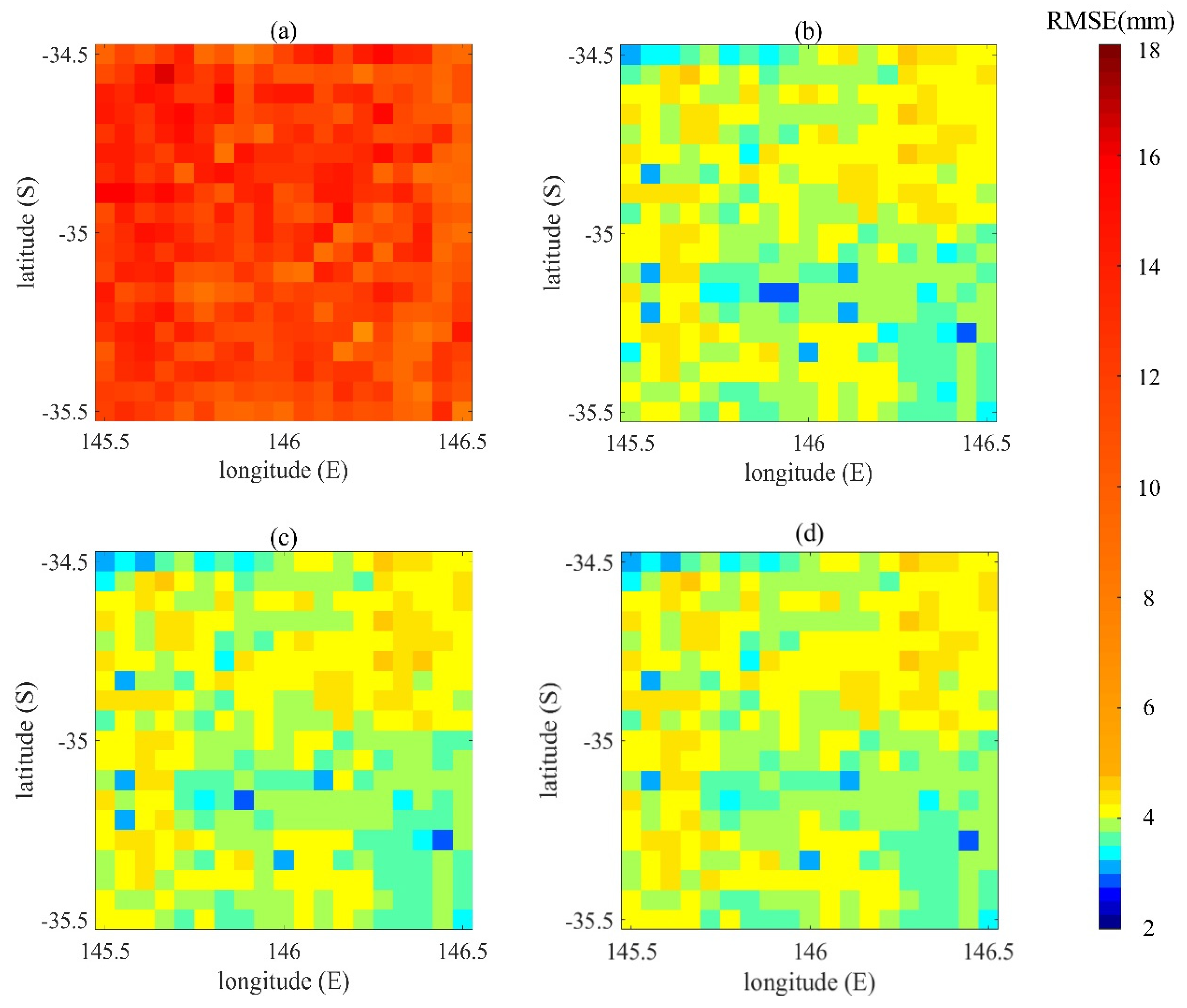
Figure 4 shows the RMSEs of the VIC simulation soil moisture values and the soil moisture analysis values obtained from the data assimilation experiments of different breeding lengths, using the CCI data for validating the results. Data assimilation using the BGM method could effectively improve the accuracy of estimation of the soil moisture and the RMSE values of data assimilation using different model breeding lengths are similar (
Figure 4). From the above experimental results, we found that although there are differences between the results of data assimilation experiments at different breeding lengths, the 72 h breeding length has a better perturbation effect on the EnKF data assimilation and the generated soil moisture estimation data had the smallest value of RMSE.
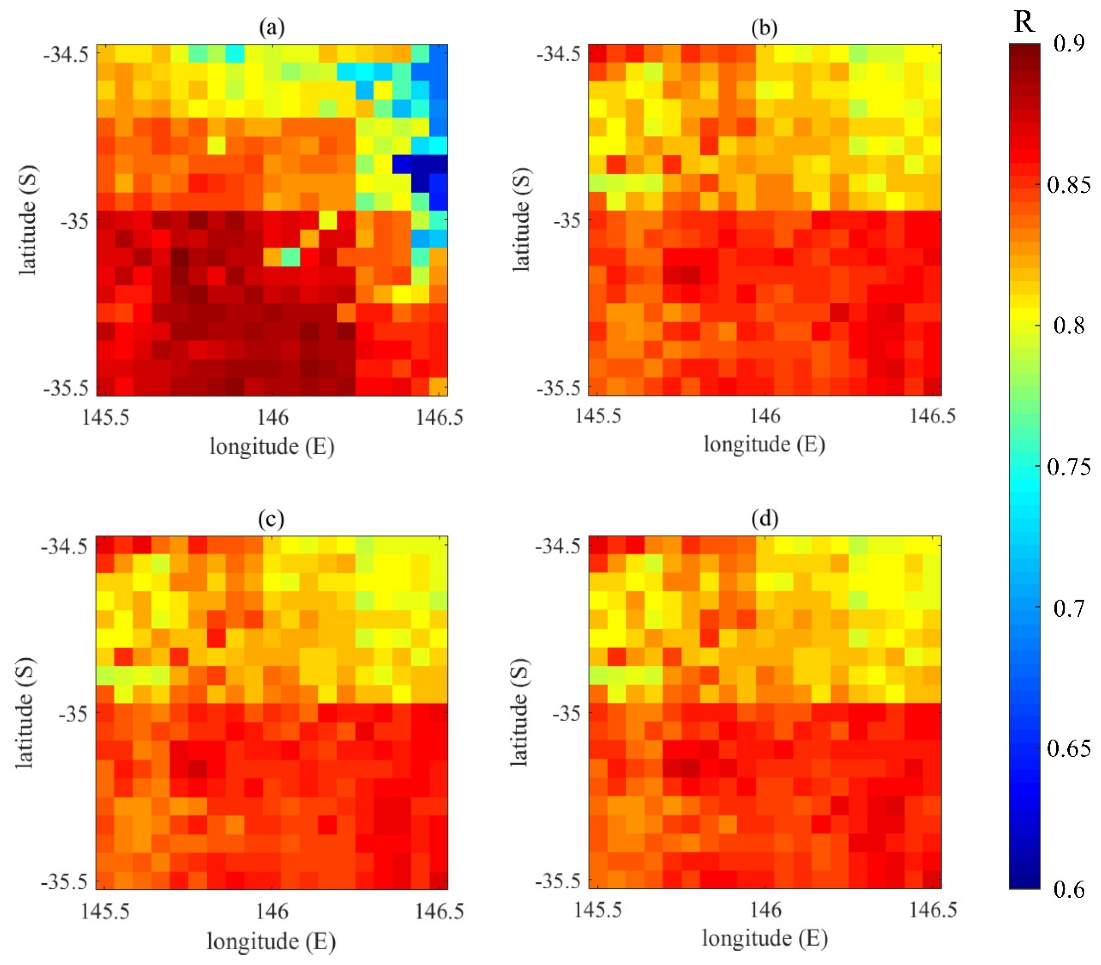
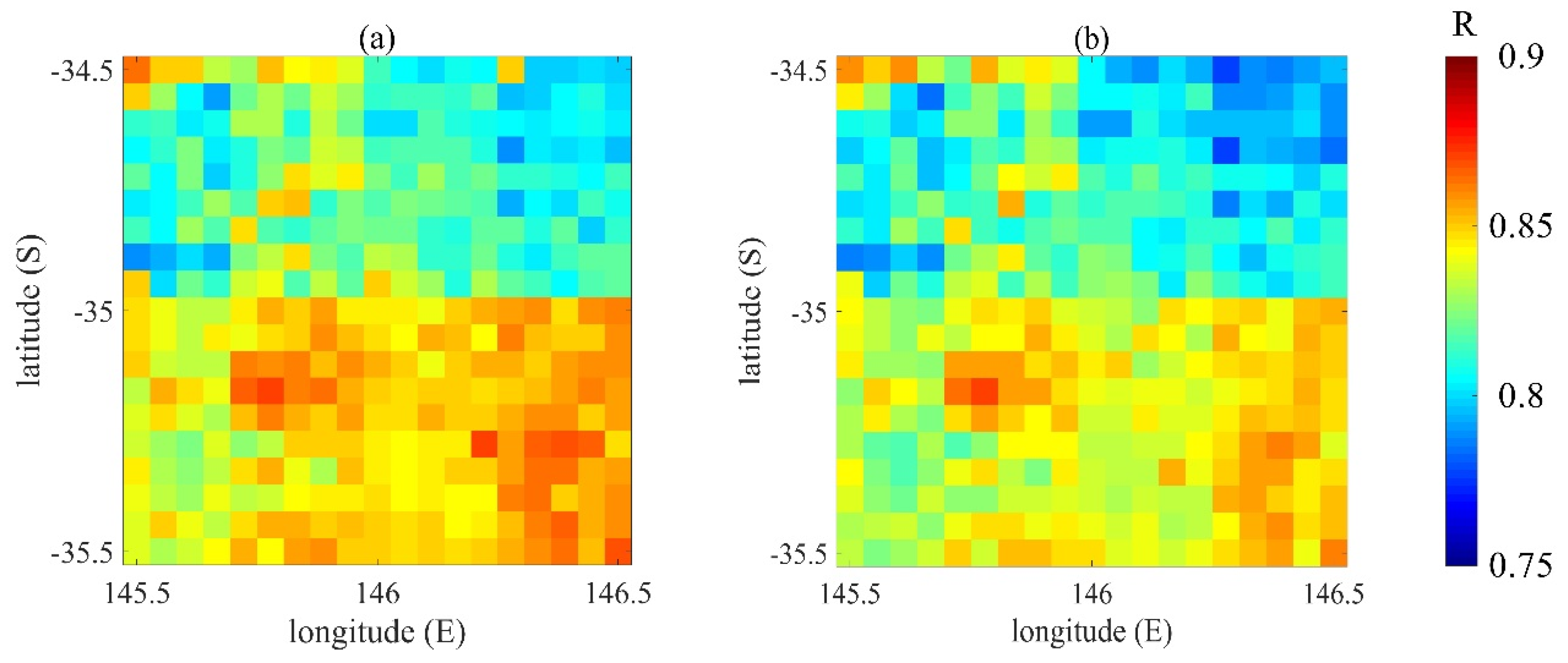
Figure 5 shows the correlation coefficient R between the data assimilated soil moisture analysis values with different breeding lengths and the CCI data.
Table 3 shows the accuracy of the soil moisture estimation results of the four sets of experiments using the CCI data. From
Figure 5, we find that the correlation coefficient of the southern region is slightly higher than that of the northern region, indicating that the data assimilation results of the study area are slightly better than that of the northern region. The highest value of the RMSE of the four experimental sets is the RMSE mean of the VIC simulation experiment, which is 11.9075. Compared with the VIC simulation experiment, the RMSE means of the three sets of data assimilation experiments have significantly improved, which proves that data assimilation using the BGM method could improve the estimation accuracy of the soil moisture. Among the four sets of experiments, the mean and variance of the RMSE of the data assimilation experiment with the breeding length of 72 h are the smallest, indicating that this result was more accurate. The mean values of R for all the experiments are above 0.8. The mean and variance of R of the three groups of data assimilation experiments are very close.
Through the above experiments, the soil moisture analysis values obtained from the initial field generated by the BGM method with different breeding lengths were analyzed and evaluated. It was found that compared with the 24 h and 48 h breeding time, the perturbation effect of the EnKF data assimilation with 72 h breeding time is better and the generated soil moisture estimation data have smaller RMSE and larger R, which is more consistent with the verification data.
4.2. The Effect of Ensemble Sizes on Data Assimilation
The EnKF performs the estimation of the background error covariance matrix by the statistical simulation of a finite ensemble of members; hence, different ensemble sizes have a significant influence on the data assimilation results. If the size of the ensemble members is too small, the background error covariance will be unrealistically small and eventually lead to filter divergence, which makes data assimilation impossible; if it is too large, the efficiency of data assimilation will be significantly affected. Therefore, the size of the ensemble plays an important part in the EnKF perturbation. We take data assimilation with ensemble sizes of 20, 50, 100, 200, and 500 to evaluate the soil moisture analysis values obtained by using different ensemble sizes for data assimilation.
Based on the conclusions of the experiments on the effects of different breeding length perturbations on the EnKF data assimilation (see
Section 4.1), we uniformly set the breeding length to 72 h. The BGM method was used to generate a set of ensemble sizes of 20, 50, 100, 200, and 500, and data assimilation experiments were performed. The experimental results were validated using the CCI observation data. The data assimilation time range is from 1 March 2016 to 31 December 2016 (305 days).
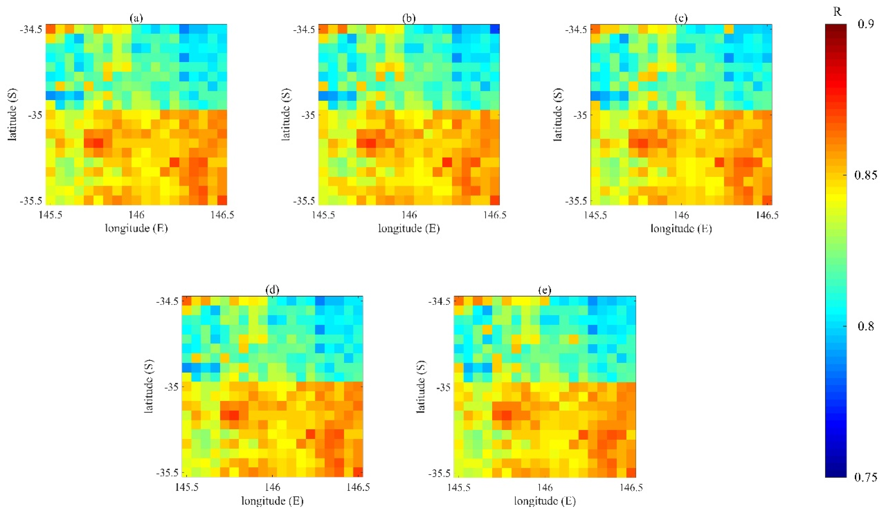
Figure 6 shows the RMSE of the soil moisture analysis values obtained from the data assimilation experiments of different ensemble sizes, compared with the CCI data. The correlations (R) between the observations and the results from data assimilation with different ensemble sizes are shown in
Figure 7.
Table 4 shows the accuracy of soil moisture estimation results for the five sets of experiments with different ensemble sizes. We found that using the BGM method to generate the initial field, even for small ensembles, could still obtain good soil moisture estimates. The appropriate ensemble size does not affect the efficiency of the data assimilation procedure. It could express the background field error well and could prevent the filter from diverging. When the ensemble size is 100, the RMSE mean is small and the variance is comparable to the data assimilation experiments of the other ensemble sizes. Through the mean and variance of RMSE and R, we found that when using the BGM method to generate ensembles of different sizes for data assimilation, the obtained data assimilation results are different, but those differences are not very big. Therefore, we chose the ensemble size 100 for data assimilation to ensure the efficiency and accuracy of the soil moisture estimation for data assimilation.
4.3. Comparison of Data Assimilation Experiments
As shown in
Section 4.1 and
Section 4.2, we have determined the breeding length and initial field ensemble size of the BGM method. Now, we use these values to conduct experiments using the BGM and the MC method and compare the accuracy of the soil moisture estimation between the two methods. The CCI observation data and in situ data from 13 locations in the study area were used to validate the data assimilation results. The RMSE and R were calculated to quantitatively evaluate the different data assimilation results.
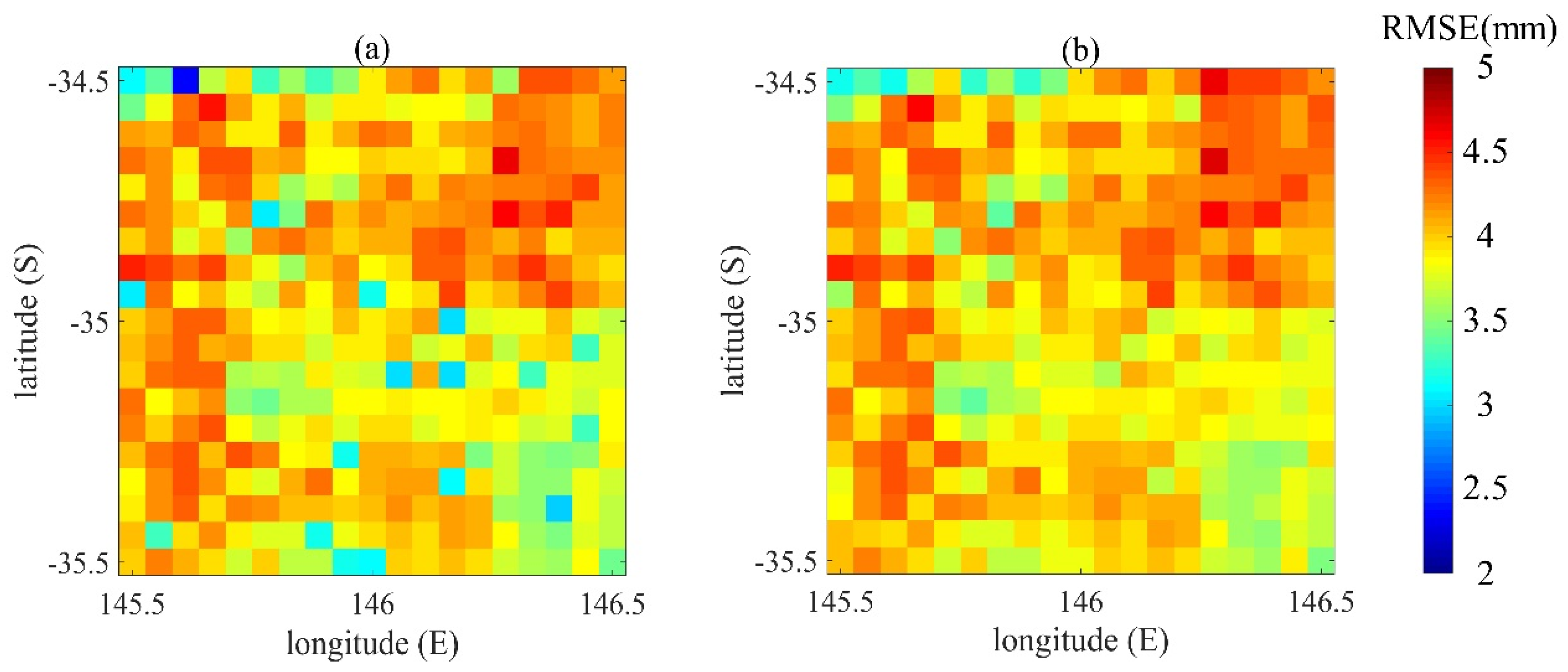
Figure 8 shows the RMSE and
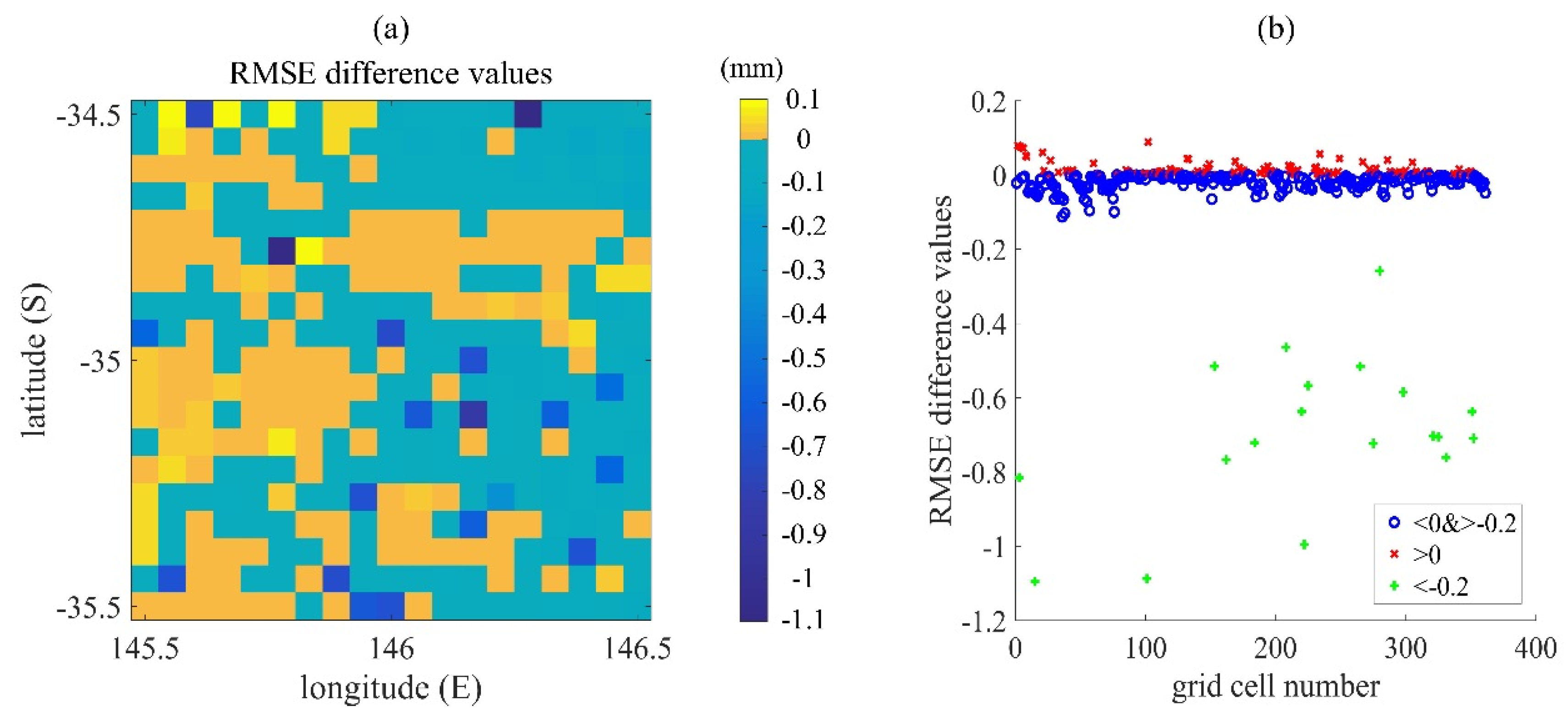
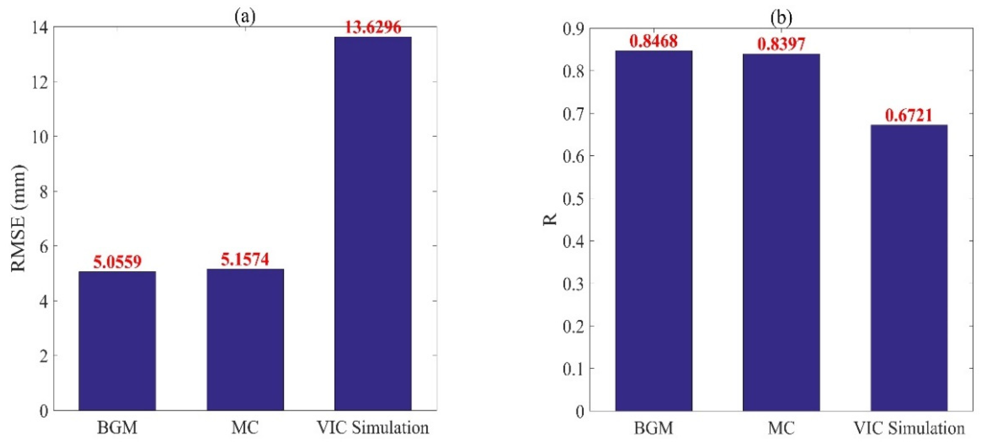
Figure 9 shows the R between the CCI data and the soil moisture analysis values obtained by the data assimilation experiment, using different perturbation methods. The RMSE mean of the soil moisture estimation results obtained by data assimilation using the BGM method is 3.9458 and that using the MC method is 3.9911. The R mean of soil moisture estimation results obtained by data assimilation using the BGM method is 0.8343 and using the MC method is 0.8272. The accuracy of the soil moisture analysis values obtained from data assimilation using the BGM method is better than that obtained using the MC method. To accurately characterize the influence of different perturbation methods on the estimation accuracy, we calculated the deviation between the RMSEs of the two assimilation methods, that is, the RMSE of the data assimilation analysis value and the true value of the BGM method, minus the RMSE of the data assimilation analysis value and the true value of the MC method, δ
RMSE = RMSE
DA(BGM) − RMSE
DA(MC). If δ
RMSE is negative, the estimation accuracy of the BGM method is higher than that of the MC method; if δ
RMSE is positive, it is proved that the estimation accuracy of the MC method is higher than that of the BGM method. The specific results are shown in
Figure 10.
The blue area shows negative values and the yellow area shows positive values. The number of grids in the blue region is 248, accounting for 68.7% of the total number of grids. The minimum value in the blue region is –1.0952 mm, which proves that the RMSE of the BGM method is smaller than the RMSE of the MC method by 1.0952 mm. The number of grids in the yellow area is 113, accounting for 31.3% of the total grid number and the maximum value of the yellow area is 0.0885, which proves that the RMSE of the MC method is smaller than the RMSE of the BGM method by 0.0885 mm. In
Figure 10b, the red point is positive and the blue and green points are negative. Most of the points are distributed around the value of 0, where there are more blue points than red, which proves that the BGM method is better than the MC method in most of the grids. The green dot represents a grid point with δ
RMSE < –0.2 mm and has a total of 19 grid points, accounting for about 0.05% of the total grid points. These points represent a significant improvement in the data assimilation ability of the BGM method compared with the MC method. It is proved by experiments that the BGM method is better than the MC method in data assimilation perturbation and could improve the accuracy of the data assimilation for soil moisture estimation.
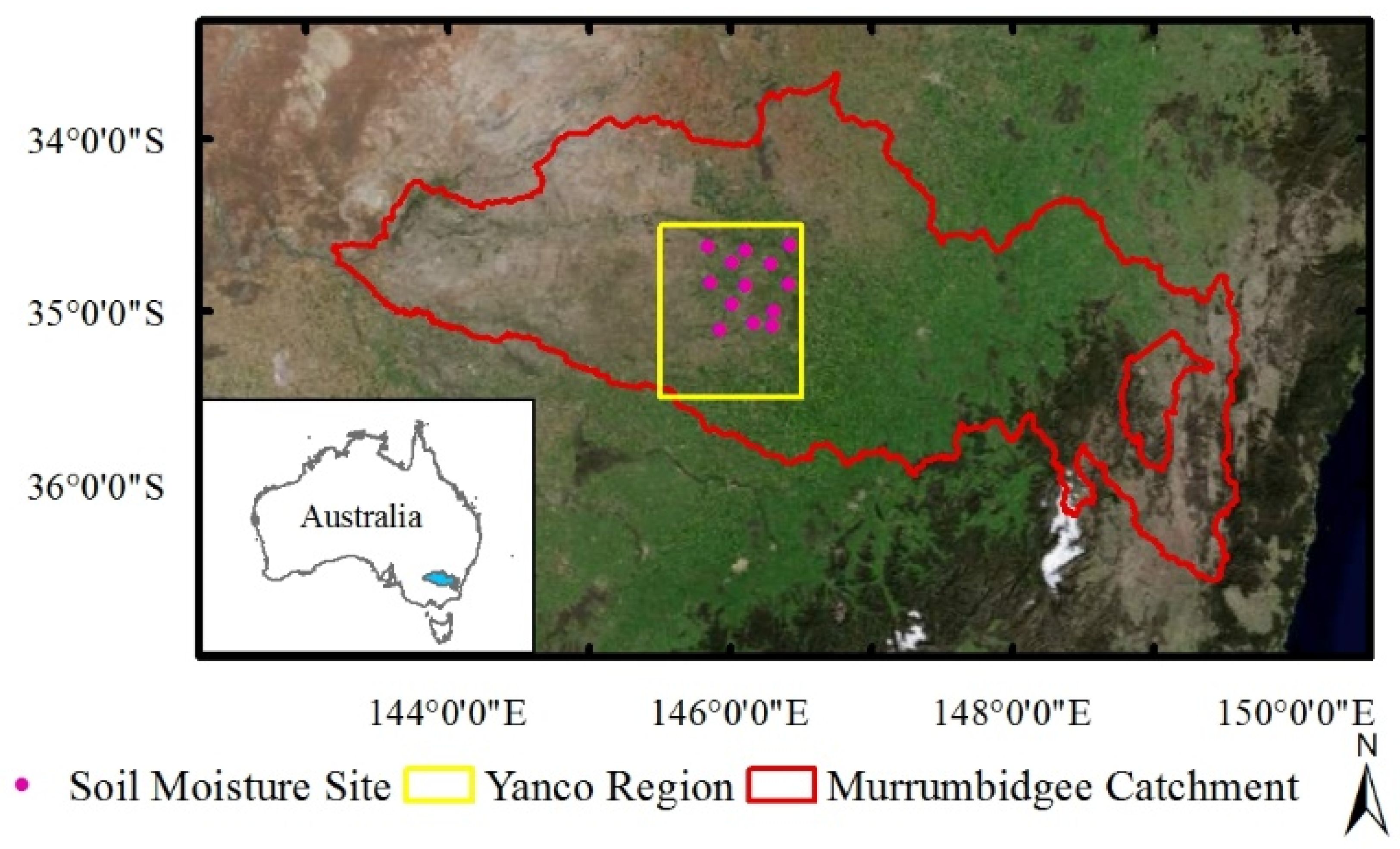
In addition to the validation with the CCI observation data, we also use data from 13 in situ stations in the study area. Since the Y3 site had no soil moisture data in 2016, we verified the experimental results using the remaining 12 sites excluding the Y3. Site data can only represent point-scale soil moisture observations, so we used the site data to verify the soil moisture analysis values of the grid where the site is located.
Figure 11 and
Table 5 clearly show that the data assimilation could significantly improve the accuracy of the soil moisture estimation compared with the soil moisture simulated by the VIC model. Among them, the soil moisture analysis value obtained by data assimilation using the BGM method is more accurate than the MC method data assimilation. Based on the data assimilation experiments corresponding to the 12 in situ sites, the RMSE of the analysis values using the BGM method at the 10 sites (Y1, Y2, Y4, Y5, Y6, Y7, Y10, Y11, Y12, and Y13) are better than the RMSE of the data assimilated values obtained using the MC method. The two assimilated values at the Y6 site had the largest RMSE deviation of 0.8500. The RMSE of the MC method data assimilation analysis values at the Y8 and Y9 sites is better than the RMSE of the values obtained using the BGM method. In the 12 sites of the study area, the average of the RMSE of the BGM method analysis values was reduced by 0.1015, compared with the average RMSE of the MC method values. For the grids corresponding to the 12 sites, the R of the BGM method analysis value is greater than the R of the MC method value. The average value of R of the BGM method data assimilation analysis value increased by 0.0071 compared with the average value of R of the MC method data assimilation analysis value. The experiment proves that the accuracy of the data assimilation analysis value obtained using the BGM method is higher than obtained using the MC method.
5. Discussion
We argue that a more accurate estimate of the soil moisture could be obtained using the BGM method to perturb data assimilation compared to the MC method. The BGM method uses the model loop to describe the growth of error in the model, so that the perturbation field contains not only the initial field error information, but also the model error information. As a purely statistical initial field perturbation method, the MC method could only generate random numbers obeying the standard distribution to represent the error. Therefore, the MC method usually assumes that the random errors of the initial field and the background field obey the standard Gaussian distribution. The BGM method uses the model to breed the error and uses the model to appropriately adjust the form of the error distribution, so that the error distribution is more in line with the true error distribution state.
As pointed out by Renzullo et al. [
31], implementation of the EnKF does not explicitly represent the model error. The EnKF data assimilation based on the BGM method proposed in this study provides a new idea to consider the model error during error estimation of data assimilation. The BGM method allows the model to participate in the perturbation of the initial field and the error term
w so that the model information is completely absorbed by the ensemble, and the EnKF data assimilation completes the expression of the model error. We used two sets of experiments to address the two key issues: the breeding length and ensemble size in the ensemble perturbation and data assimilation. We performed a quantitative analysis of the data assimilation experiments using different breeding lengths (
Section 4.1), and found that a breeding time of 72 h produced the most accurate soil moisture estimates. When the breeding time is too long, the accuracy of the data assimilation is not significantly improved; however, longer breeding times have a significant impact on experimental efficiency. We also conducted experiments with the BGM method using different ensemble sizes (
Section 4.2). Different ensemble sizes lead to differences in the data assimilation results, but this difference is not significant, because the perturbation field generated by the BGM method could completely express the random error and the model error of the initial state of the soil moisture. The choice of the ensemble size should not only be considered in terms of the accuracy of the soil moisture estimation, but also the efficiency of data assimilation. The expansion of the ensemble size will reduce the efficiency of data assimilation and increase the running time. Therefore, on the basis of balancing operational efficiency, we chose an ensemble size of 100 as the ensemble size option for the BGM method experiment.
In order to fully verify the accuracy of the EnKF data assimilation framework based on the BGM method, we used in situ data from 13 locations in the study area as the main verification data to validate the data assimilation of two different perturbation methods. The in situ stations in the study area were located sparsely, which limited the verification of large-scale soil moisture data. Therefore, we set the spatial resolution of the data assimilation analysis value as 0.05°, so the data assimilation analysis value would be closer in spatial resolution with data from sites, and the verification result of the site data for soil moisture could be more accurate and reasonable. The in situ data cannot afford the verification for the data assimilation analysis value in all the study areas, so we use CCI data as auxiliary data. The data precision of CCI data in Yanco area is high enough to support verification [
18]. In 2016, the overall coverage rate of CCI data in Yanco area was 94.30%, which provides enough samples as validation data. The difference in spatial resolution between datasets would result in uncertainty, but giving that the soil moisture analyzed value validation we performed is between the site and CCI data, the verification results of this paper are still objective and reliable.
The experimental comparison of the data assimilation using two different sets of perturbation methods (see
Section 4.3) shows that the initial perturbation obtained by the BGM method is more suitable for the initial field and error term
w of the disturbance data assimilation, compared with the initial perturbation obtained by the MC method. The accuracy of the soil moisture analysis value estimated by the BGM method is higher than that estimated by the MC method. The EnKF data assimilation theory framework based on the BGM method proposed in this study could improve the estimation of soil moisture. The theoretical framework uses the BGM method to breed the perturbation field so that the initial field and the error term
w contain the model information. The perturbation field bred by the BGM method is used to perturb the initial field error and the background field error of the EnKF so that the soil moisture estimation of the EnKF data assimilation could be accurately adjusted.
6. Summary and Conclusions
This study proposes using the BGM method for the EnKF data assimilation in relation to the perturbation of land surface data assimilation. The BGM method is widely used in meteorological numerical prediction and atmospheric data assimilation. This paper introduces the BGM method and applies it to land surface data assimilation, using the BGM method to generate the initial field of the EnKF and the error term w of the prediction step in the EnKF, so that the perturbation ensemble completes the error expression in the EnKF data assimilation. The advantages of using the BGM method are: (1) The BGM method uses the model in breeding the mode so that the initial field and error term w of the data assimilation not only represent the initial field error, but also contain relevant information of the model error; (2) Adjust the ensemble distribution pattern of the initial field and the error term w to make it more in line with the error distribution state under real conditions (the soil moisture error distribution in the actual state does not necessarily strictly obey the standard Gaussian distribution). In this study, the BGM method is used to perform the EnKF data assimilation and the problem of the BGM perturbation mode breeding length and ensemble size is experimented. Finally, the experimental comparison with the MC method proves the applicability and superiority of the BGM method in land surface data assimilation.
The results of the validations done using the CCI remote sensing data and in situ data are different because the accuracy of in situ data is high, but its spatial resolution is point scale and the spatial resolution of the analysis values is different. The CCI data are consistent with the spatial resolution of the analysis values, but the accuracy of the CCI data is not as good as the in situ data. The data assimilation results of the two perturbation methods used in this experiment have significantly improved the accuracy of the soil moisture estimates compared to the results from the VIC model simulation. The data assimilation uses accurate observation data to correct the simulated values of the model; therefore, the data assimilation results are more accurate. Even when the accuracy of the observation data is not ideal, the accuracy of the analysis value of the BGM method EnKF data assimilation is still reliable and needs to be further explored in future research.
In this study, we propose an EnKF data assimilation framework based on the BGM method. It is experimentally proven that the BGM method could effectively generate the data assimilation initial field, perturbation error term w, and improve the estimation accuracy of the data assimilation of soil moisture. In future research, we plan to extend the EnKF data assimilation framework based on the BGM method in the following ways: (1) discuss the influence of the framework on the unbiased of the EnKF state estimator. (2) evaluate whether the BGM method is applicable to data assimilation on a global scale and (3) analyze the applicability of the BGM method to other Kalman filter data assimilation methods.


