Article

Gap-Filling of a MODIS Normalized Difference Snow Index Product Based on the Similar Pixel Selecting Algorithm: A Case Study on the Qinghai–Tibetan Plateau

1
State Key Laboratory of Remote Sensing Science, Jointly Sponsored by Beijing Normal University and the Institute of Remote Sensing and Digital Earth of the Chinese Academy of Sciences, Beijing 100875, China
2
School of Geographical Sciences, Qinghai Normal University, Xining 810016, China
3
Institute of Remote Sensing Science and Engineering, Faculty of Geographical Sciences, Beijing Normal University, Beijing 100875, China
4
State Key Laboratory of Earth Surface Processes and Resource Ecology, Beijing Normal University, Beijing 100875, China
*
Author to whom correspondence should be addressed.
Submission received: 12 March 2020 / Revised: 23 March 2020 / Accepted: 24 March 2020 / Published: 27 March 2020
(This article belongs to the Section Remote Sensing in Geology, Geomorphology and Hydrology)

Abstract

:
Cloud contamination has largely limited the application of the Moderate Resolution Imaging Spectroradiometer(MODIS) normalized difference snow index (NDSI). Here, a novel gap-filling method based on spatial-temporal similar pixel interpolation was proposed to remove cloud occlusions in MODIS NDSI products. First, the widely used Terra and Aqua combination and three-day temporal filter methods were applied. The remaining missing NDSI information was estimated by using similar eligible pixels in the remaining cloud-free portion of a target image through a spatial-temporal similar pixel selecting algorithm (SPSA). The MODIS daily NDSI product data from 2003 to 2018 in the Qinghai–Tibetan Plateau (China) was used as a case study. The results demonstrate that the three-step methodology can generate almost completely cloud-free, daily MODIS NDSI images, reducing the cloud-gap fraction from >45% to less than 1.5% on average. The validation results of the SPSA method exhibited a high accuracy, with a high R2 exceeding 0.78, a low mean absolute error of 2.77%, a root mean square error of 3.78%, and a 96.92% overall accuracy. The proposed method can fill cloud gaps without a significant loss of accuracy, especially during snow cover transition periods (autumn and spring), which may provide more accurate cloud-free NDSI data for climate change and energy balance studies.

Graphical Abstract

1. Introduction

As an integral part of the Earth’s climate system, seasonal snow is one of the most variable land cover types throughout the year and has a strong impact on the radiation and energy balance, hydrological and biogeochemical cycles, and even human activities [1,2]. Snow cover characteristics, such as the cover extent and duration, are also crucial parameters in hydrological and ecological process models [3]. Moreover, meltwater from glaciers and seasonal snow packs provide water for nearly one-sixth of the world’s population [4] and more than one-fifth of China’s population, with the Tibetan Plateau being the main source of meltwater in China. Therefore, in recent years, the study of snow distribution and its spatiotemporal changes has become the focus of numerous studies [5,6,7,8,9,10,11,12,13], such that the timely and accurate acquisition of snow distribution information has become critical [9,14,15].
Satellite images acquired using remote sensing can provide continuous spatiotemporal information on snow coverage over long time series and on a global scale, which is advantageous to a large number of researchers [16,17,18,19,20,21,22]. Among other widely-utilized snow cover assessment methods, MODIS products have become one of the main data sources for ice and snow research due to their global coverage, long time series (i.e., the databases are currently updated and have been maintained since 2000), high spatial (e.g., 500 m) and temporal (e.g., daily) resolutions, and free access, which allow for real-time, accurate, and large-scale snow cover variation monitoring [14]. Extensive studies [23,24,25,26,27,28] have demonstrated that MODIS products exhibit an excellent snow extraction performance, with an overall accuracy exceeding 90% under clear-sky conditions. Nonetheless, cloud occlusion in MODIS snow cover products often leads to numerous data gaps, which hinders their promotion and adoption in environmental research.
A large number of algorithms have been developed to improve the spatiotemporal continuity of MODIS snow products over the past decade [14,25,29,30,31,32,33,34,35,36,37,38,39,40,41,42]. Traditional cloud removal algorithms can be divided into four types: temporal, spatial, spatiotemporal, and multi-source fusion methods [14].
The Terra and Aqua combination (TAC) method is the simplest and most transparent of the temporal methods [40,43,44,45] and has, thus, become the most popular temporal approach. The TAC method can decrease the cloud-gap fraction (CGF) by up to 5–20% without significantly sacrificing the product accuracy [43,46]. The specific rules are the following [14]: if a pixel is cloudy in one product, but cloud-free in another (Aqua or Terra), the cloudy pixel will be updated using the classification of the cloud-free pixel. Temporal filtering is another popular temporal method that directly replaces cloudy pixels using information from previous or subsequent day (or days) pixels [21]. However, since snow cover is assumed to remain constant throughout a given temporal interval, the accuracy in snow-transitional periods is lower than that in snow-stable periods [47].
Furthermore, the spatial filter (SF) and snow line (SNOWL) approaches are among the main spatial methods, of which the most common is the SF [39,40,48]. This method consists of replacing a cloudy pixel by using four or eight neighboring non-cloud pixels [14]. The SNOWL method [13,38], which is also known as the snow transition elevation method [39,49], reclassifies the cloudy pixels as snow or land according to the snowpack elevation distribution; cloudy pixels above the snow line will be classified as snow, while those below the snow line will be classified as land.
The spatiotemporal method combines the spatial and temporal methods alternately and successively [21]. Therefore, this method is essentially a combination and extension of the temporal and spatial methods.
Substitution is the essence of the above methods, i.e., finding cloud-free pixels to replace cloud-covered pixels. Except for the snowline method, these methods have the following common limitations: (1) The cloud-free pixel used for replacement is typically near the cloudy pixel, regardless of the difference in time or space. In other words, the selection of non-cloud pixels is limited by distance. Regarding the time difference, the time window is typically set to 2–7 days. In a spatial neighborhood, the distance is even smaller, with a spatial window of only 3 × 3 pixels. (2) The prediction accuracy tends to decrease with increasing distance [50], such that users must make a tradeoff between de-clouding accuracy and de-clouding efficiency.
The multi-source data fusion method entails the fusion of MODIS products and microwave remote sensing data (e.g., Advanced Microwave Scanning Radiometer on Earth Observing System, AMSR-E/AMSR-2). Although this method can remove all cloud contamination, large errors are also introduced due to the coarse resolution of microwave remote sensing [30]. Wang et al. [43] also report that the accuracy of this method is more dependent on the accuracy of the AMSRE product itself.
Currently, two versions of the MODIS daily snow product have been widely used in most studies (i.e., version 5 [51] and version 6 [52]). In version 5, the binary and fractional snow cover are provided, where both of which are calculated based on the normalized difference snow index (NDSI) through a specific threshold for binary snow cover products [53,54] or a linear regression relationship for fractional snow cover (FSC) products [55]. In 2016, MODIS version 6 was released, which no longer provides binary snow cover products but instead offers NDSI products, which can be regarded as continuous numerical products [52,56]. Compared with binary snow cover products, NDSI products can provide more information, which is more conducive to hydrological and ecological process simulations. Additionally, the increased data content (NDSI product) allows for flexibility in using the datasets for specific regions and end-user applications [56]. However, traditional cloud removal methods have mainly focused on cloud removal for discrete MODIS binary snow cover products (i.e., snow or snow-free). Currently, there are relatively few studies on cloud removal algorithms for continuous snow cover products (such as the NDSI product in version 6), and there have not been many studies that have performed cloud removal for fractional snow cover (FSC, V5) products. Dozier et al. [42], for example, first applied the spatiotemporal cube concept to snow products in 2008, filling in the gaps in the cloud by interpolating cubic splines in time on each pixel. Tang et al. [25] also used the cubic spline interpolation algorithm to de-cloud MODIS FSC products monitoring the Qinghai–Tibetan Plateau. Dozier’s algorithm, however, considers only a small number of local neighbors; Tang’s algorithm is a simple one-dimensional time interpolation algorithm that only considers the time information associated with snow cover and does not include the spatial characteristics of snow cover. In the case of a substantial number of continuous cloud cover days, a large number of outliers will be generated.
Dong et al. proposed a cloud removal algorithm for binary snow cover products based on station observations and optical data, whereby the conditional probability that a given cloudy pixel represents snow cover can be calculated to reclassify the residual cloudy pixels [36,57,58] on the condition that the snow depth (SD) is higher than zero at a nearby station [14]. The presence of snow in one cloudy pixel can be predicted with data from neighboring weather stations. This method has been reported as effective, especially during snow season [36,57,59]; however, the distribution and number of meteorological stations limit, to a certain degree, the predictive ability of the snow cover reconstruction [14]. Cheng et al. [60] developed a novel approach based on a similar pixel replacement method. A spatiotemporal Markov random fields (STMRF) function was developed to identify the most appropriate cloud-free pixels to replace a cloudy pixel in MODIS land surface temperature products. Hou et al. [30] further developed Cheng’s algorithm, applied it to MODIS FSC snow products, and conducted experiments in Xinjiang (China), which yielded good results. The validation results based on cloud mask assumptions exhibited a high accuracy, with a high R2 exceeding 0.8, a lower root mean square error (RMSE) of 0.1, an overestimation error (Equation (13)) of 1.13%, an underestimation error (Equation (14)) of 1.4%, an overall accuracy (Equation (12)) of 93.72%, and a spatial efficiency of 0.78 [30].
Here, we propose a novel gap-filling method based on non-local spatiotemporal similar pixels and conditional probabilities to eliminate cloud occlusion in daily MODIS NDSI products. This algorithm first determines the possible NDSI range of cloudy pixels through spatial similarity, after which, the temporal similarity is used as an index to select similar pixels in the cloud-free areas to fill the cloud-covered area in the MODIS NDSI products. Therefore, our study focuses on the following three goals: (1) a comprehensive assessment of cloud contamination severity in MODIS NDSI products (version 6) across the Qinghai–Tibetan Plateau (TP); (2) an evaluation of the potential applicability of existing widely-used binary product-based cloud removal methods to continuous NDSI products; and (3) the development and accuracy assessment of an innovative cloud removal algorithm based on spatiotemporal pixel similarity.

2. Study Area and Data
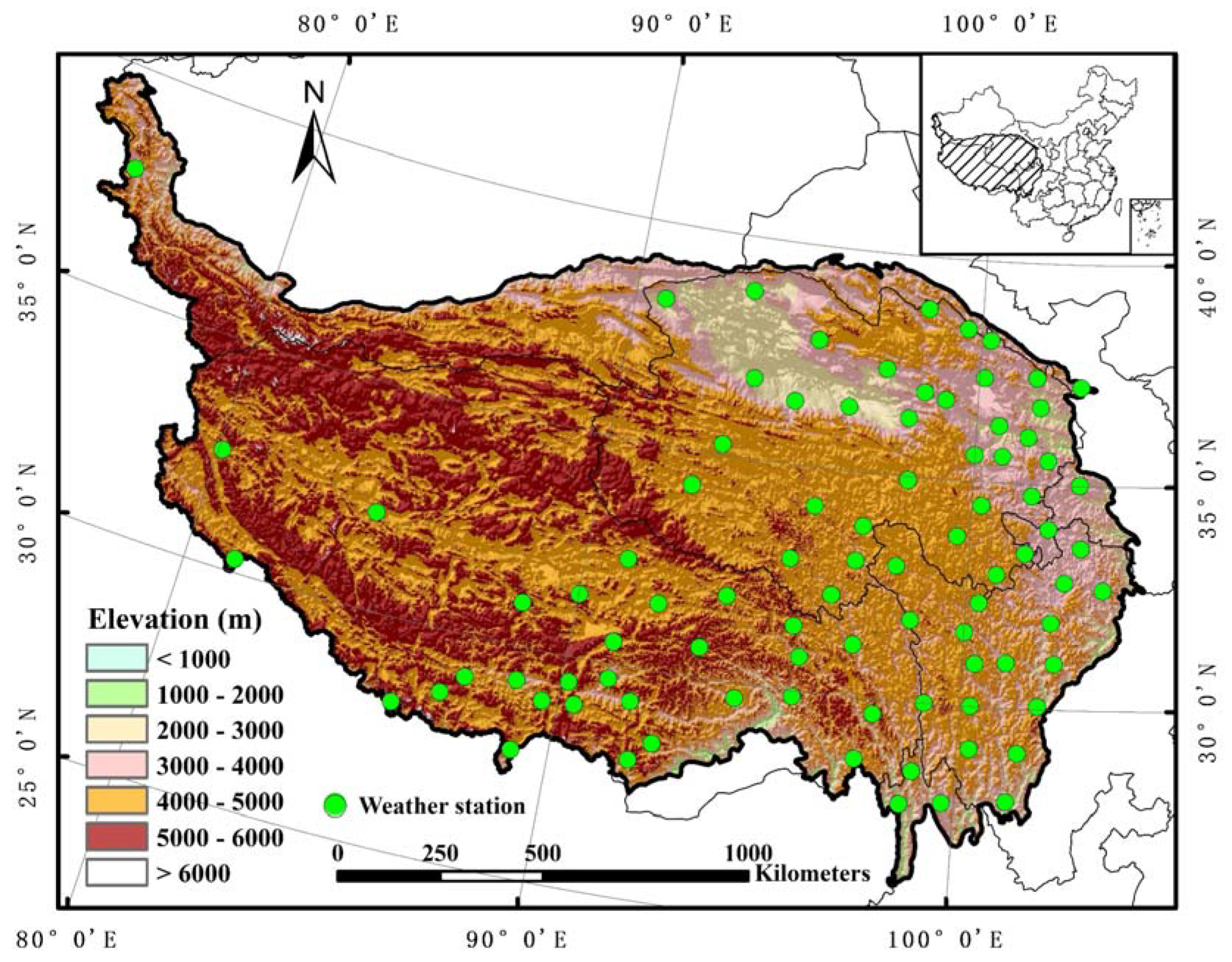
2.1. Study Area

The Qinghai–Tibetan Plateau (TP) is located in the central Eurasian continent. It ranges 1532 km from north to south (26°00′12″N to 39°46′50″N) and 2945 km from west to east (73°18′52″E to 104°46′59″E), covering an area of over 2.5 million km2 (Figure 1). The TP has a mean elevation exceeding 4000 m above sea level (m.a.s.l.) and is among the areas most sensitive to global climate change [61]. The TP features a wet and warm summer (from June to August) and a cool and dry winter (from December to February) [62]. Winter temperatures exhibit a large spatial variation, ranging from −25 °C in the west to −15 °C in the east [63], providing favorable conditions for the preservation of snow cover. Summer temperatures across the TP are generally above 0 °C; however, due to very high altitudes and low temperatures (given the decreasing rate of temperature with altitude), the abundant precipitation in the summer still causes snowfall in high altitude areas. In the southeastern TP, the East Asian Summer Monsoon and Indian Monsoon produce heavy precipitation in the summer season. In the western part, westerly winds bring abundant precipitation in winter and early spring, mostly in the form of snow [64].
Unlike in northeastern China and northern Xinjiang, China, the snow cover in the TP is relatively low (less than 1 cm), where the status of the snow cover changes rapidly due to numerous factors, such as high solar radiation and high wind speeds [10], which may result in sublimation and snow drifting. In certain parts of the TP, snow cover can change substantially, even during a single day. Moreover, as it is affected by the East Asian Summer Monsoon and Indian Monsoon [62], the southeast of the TP exhibits abundant water vapor, which may lead to large amounts of cloud cover (especially in the spring and summer). In certain areas, the average annual cloud cover duration is as long as 300 days, where the maximum number of continuous cloud-covered days is greater than 20 days. The rapid change in snow cover status and high cloud-gap fraction provides significant challenges to the study of cloud removal algorithms for snow cover products across the TP.

2.2. Data

2.2.1. MODIS NDSI Products

Two versions of MODIS daily snow products have been widely used in most studies, i.e., version 5 [51] and version 6 [52]. In version 5, binary and fractional snow cover are provided, both of which are calculated based on the NDSI.
In contrast, version 6 of the product contains several significant changes. For instance, binary and fractional snow cover estimates are no longer available, while only the NDSI is provided. The NDSI snow cover for a given pixel is reported as 0–100% [52]. The pixels with the other eight codes may represent missing data (200), no decision (201), nighttime (211), inland water (237), ocean (239), clouds (250), detector saturated (254), and filled (255) [52]. There may be two main reasons for the release of NDSI products instead of binary snow products or fractional snow cover (FSC) products in version 6: First, the threshold of the binary snow cover product (or regression coefficient of the FSC product) has significant regional heterogeneity such that the global unified standard cannot achieve an optimal effect. Second, both binary snow cover products and FSC products are generated based on NDSI products, which can provide more abundant snow information. Therefore, the NDSI product released by version 6 of MODIS is more conducive to user customization.
MODIS Terra and MODIS Aqua daily NDSI products (MOD10A1 and MYD10A1, Collection 006) from 1 January 2003 to 31 December 2018 were collected from National Snow and Ice Data Center (NSIDC) (http://nsidc.org/). Six tiles (i.e., h23v05, h24v05, h25v05, h26v05, h25v06, and h26v06) were required to cover the entire TP. The MODIS Reprojection Tool was then used to mosaic each of the six tiles via a nearest neighbor resampling method and re-project them from the sinusoidal projection into the Universal Transverse Mercator (UTM zone 45) projection with the World Geodetic System 1984 (WGS84) datum at a 500-m resolution.

2.2.2. Digital Elevation Model (DEM) Data

The NASA Shuttle Radar Topography Mission Digital Elevation Model data (SRTM3, 90 m) were provided by the Consortium for Spatial Information (CGIAR-CSI) (http://srtm.csi.cgiar.org). The DEM data were mosaicked, re-projected, and resampled to achieve consistency with the MODIS NDSI images. The elevation and aspect maps were extracted from processed DEM data for further analysis. To further analyze the influence of topographical factors (e.g., elevation and aspect) on the accuracy of the proposed algorithm, the elevation from 3000 to 6000 m was divided into 31 100-m intervals (regions with an altitude greater than 6000 m were considered as one interval). Similarly, the aspect from 0° to 360° was divided into 36 10° intervals.

3. Methodology

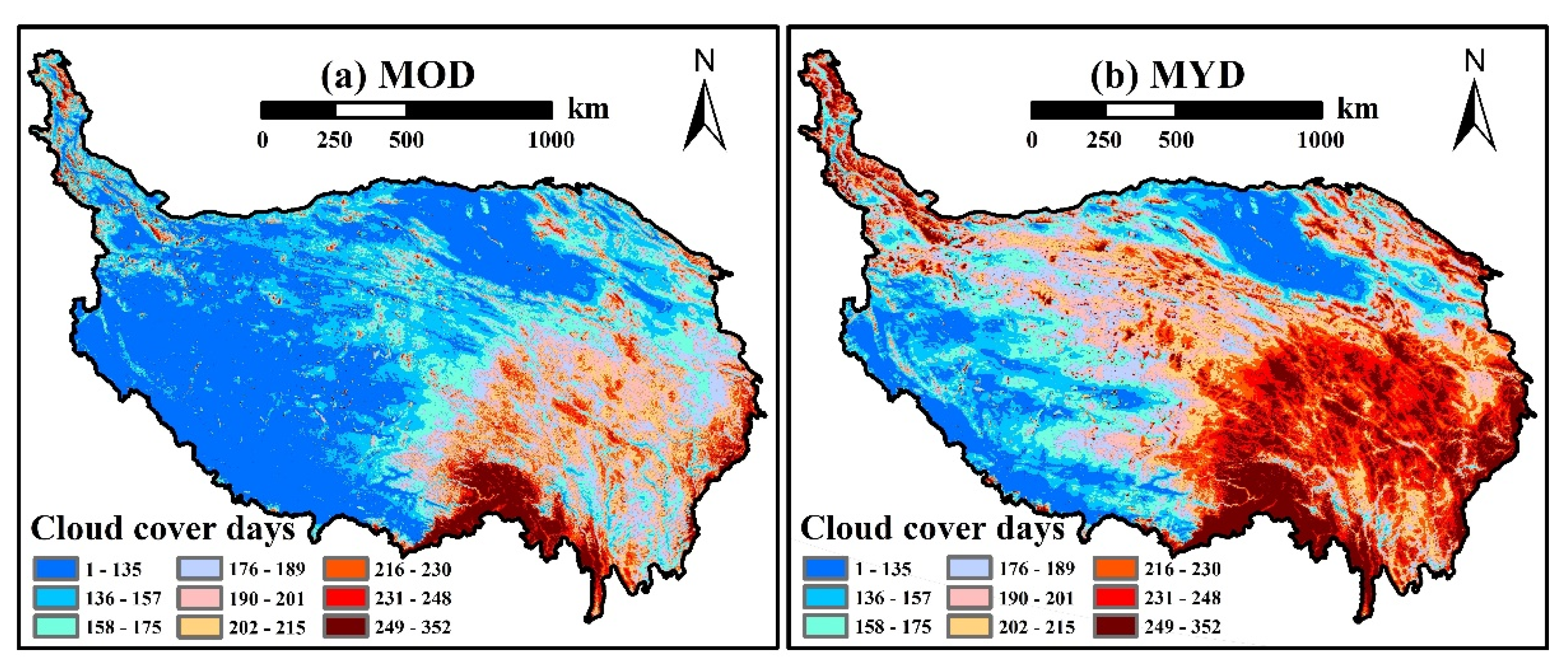
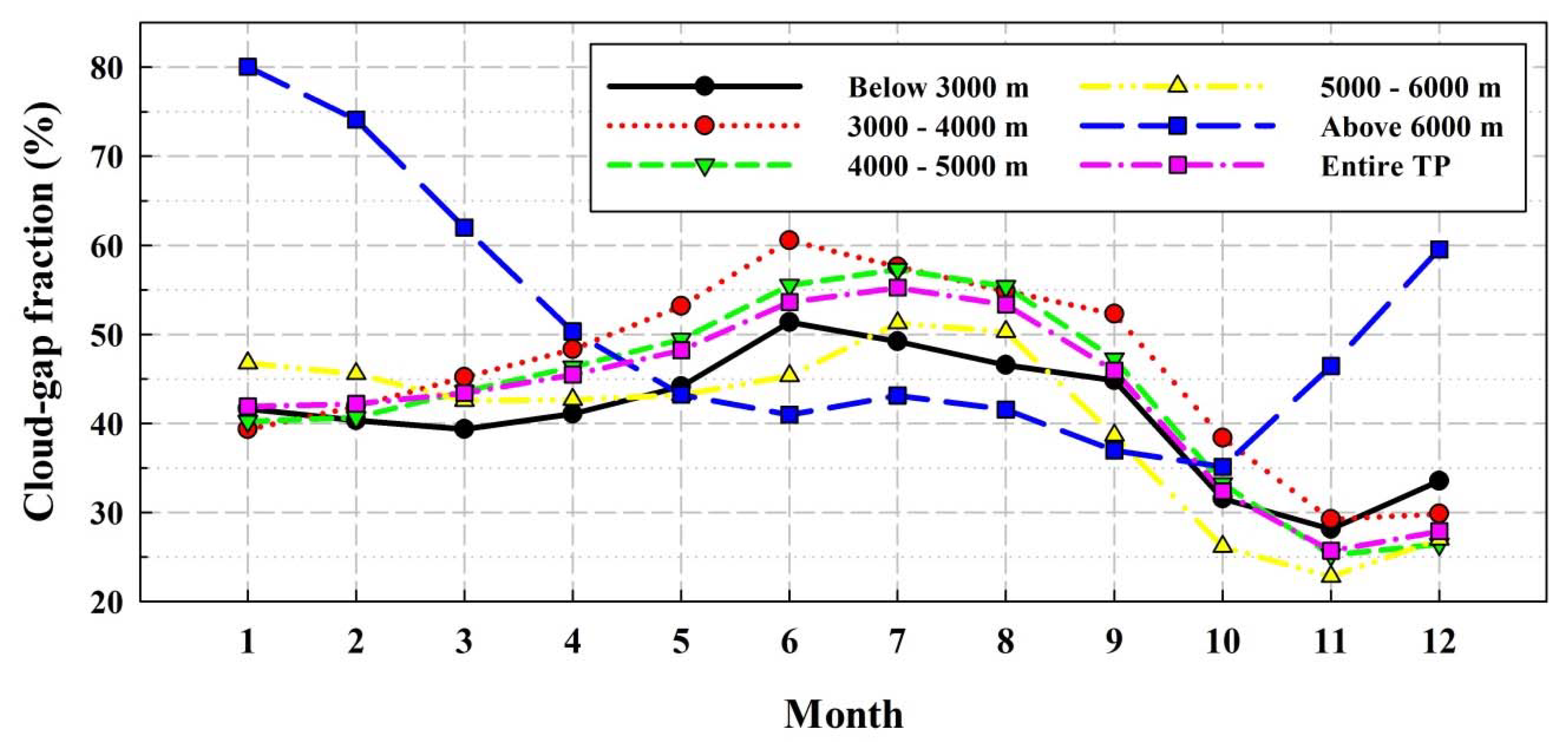
3.1. Analysis of Cloud Gaps in MODIS NDSI Products

To determine the number of cloud gaps and cloud cover duration in the MODIS NDSI products across the TP, we first reclassified the MODIS NDSI products into two categories: cloud-free (NDSI value (0 to 100), where inland water was 137), and clouds (250). Some special cases, such as detector saturated (254), missing data (200), and no decision (201), were classified as clouds due to the small amount of data available (less than 1%). After reclassification, the monthly and annual cloud coverage was calculated to analyze the influence of cloud gaps on the MODIS NDSI products across the TP.

3.2. Gap-Filling Procedure

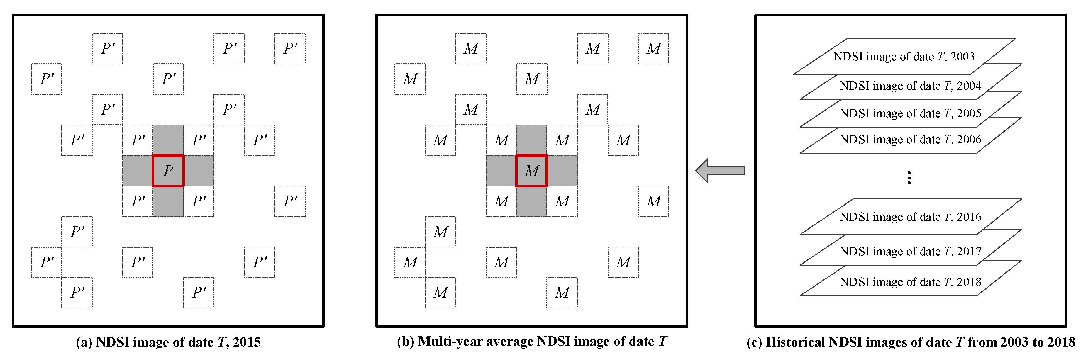
3.2.1. Theoretical Basis

Unlike construction land or vegetation (such as cropland), snow cover is less affected by human activities, and thus, is mainly influenced by natural factors, which play an important role in the formation and melting of snow. The distribution of snow cover is mainly affected by meteorological factors (e.g., moisture content, atmospheric and land surface temperature, and ocean currents), topographic factors (e.g., altitude, slope, shady slope and sunny slope, and windward or leeward slopes), and other factors (e.g., solar radiation intensity causing snow to melt, snow drifting and subsequent snow redistribution, and land-cover type causing different snow melting rates). Therefore, when the meteorological conditions, topographic conditions, and other conditions of the two pixels are very similar, the snow cover status of the two pixels, which can be measured using NDSI to some extent, might also be very similar. This similar information not only includes the local neighborhood similarity (according to the first law of geography), but also includes the non-local similarity [65,66].
When a pixel is covered by clouds, its NDSI information is lost. Fortunately, this information can be estimated from similar pixels from the remaining known region at the same date and time. Similar pixels have the following characteristics: (1) they have nearly equal mean NDSI values in a relatively small time window [30], (2) they are relatively close to each other in space [67,68], and (3) they have similar change trends in multi-temporal images [69]. Further, (4) when they are simultaneously observed, they should have close NDSI values. Thus, in this study, we selected continuous multi-temporal images to provide auxiliary information.
Figure 2 illustrates the NDSI distribution of MOD10A1 in a sample area (within 31 × 31 pixels) acquired on (a) 7 November 2010 and (b) 14 November 2010. The fifteen-day continuous NDSI values of three pixels are presented in Figure 2c. Compared with the pixel in the red box, the blue pixel better matched the trend and average value over time of the target pixel, even though it was farther away from the target pixel. Therefore, we suggest that the blue pixel was similar to the target pixel, whereas the red pixel was not.
Based on this principle, the missing NDSI values of the cloudy pixels can be calculated from similar eligible pixels in the clear sky region on the same day with the help of multi-temporal reference images [30].

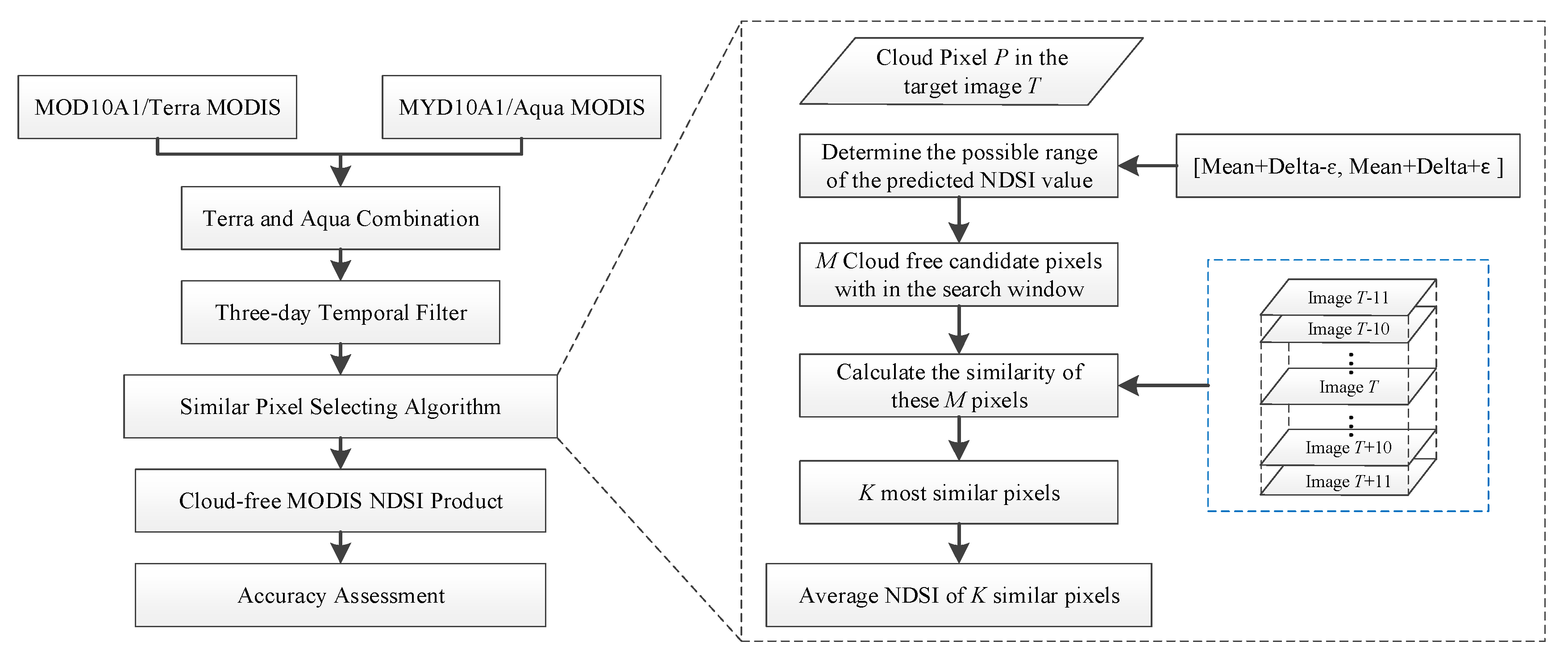
3.2.2. Gap-Filling Method

An innovative cloud removal method based on similar pixel replacement was proposed to retrieve the missing NDSI information beneath the cloud gaps in the daily MODIS NDSI products. The Terra and Aqua combination (TAC) method and a three-day temporal filtering procedure (3DTF) were executed first to fill some gaps before the application of a similar pixel selecting algorithm (SPSA). Figure 3 illustrates a detailed cloud removal procedure via the MODIS NDSI product gap-filling method.
1. Terra and Aqua Combination (TAC)
The daily MOD10A1 and MYD10A1 (hereinafter referred to as MOD and MYD, respectively) products were first combined due to the characteristics of clouds that move over time [14]. The priority was assigned to MOD, as numerous validation studies demonstrated that it had more accurate retrievals than did MYD [26,70]. The specific combination strategy was as follows [30]: when a pixel was cloud-free in both MOD and MYD, we used the NDSI value in MOD. When a pixel was cloud-free only in one of the products, we used the cloud-free NDSI value.
2. Three-Day Temporal Filter (3DTF)
Adjacent temporal filtering is based on the assumption that snow will persist on the land surface for a certain amount of time [30]. In previous studies, the size of the time filter window (days) varied from one to eight days. Due to the special climate conditions of the TP (high wind speeds easily lead to snow redistribution and a thin snow layer is easy to melt quickly), the snow state changes rapidly; therefore, a long composite period will introduce errors. In this study, the composite days were set to three days (i.e., the day of the cloud coverage, as well as the days before and after cloud coverage). When a pixel was covered by clouds and was cloudless the day before and after, the NDSI value could be calculated using the following formula:
NDSI _ predict c l o u d T   ( x , y ) = 1 2 ( NDSI _ observed c l o u d f r e e T 1   ( x , y ) + NDSI _ observed c l o u d f r e e T + 1   ( x , y ) ) ,
where NDSI _ predict c l o u d T   ( x , y ) is the predicted NDSI value of a cloud-covered pixel ( x , y ) at date T, and NDSI _ observed c l o u d f r e e T 1   ( x , y ) and NDSI _ observed c l o u d f r e e T + 1   ( x , y ) are the observed NDSI values of the clear-sky pixel ( x , y ) at dates T − 1 and T + 1, respectively.
It should be noted that the conditions for the application of 3DTF were very strict. Particularly, the predicted NDSI value of the cloudy pixel could be calculated only when the pixel was cloudless the day before and after. The input data for this step were the output products of the previous step (i.e., a daily combination of MOD and MYD).
3. Similar Pixel Selecting Algorithm (SPSA)
The SPSA can be divided into two steps: (a) determine the possible range of the NDSI and (b) search for the most similar pixels within the possible range and calculate the predicted NDSI value.
(A) Determination of the potential NDSI range
The physical process of snow accumulation and melting follows a predictable spatial pattern that occurs yearly [50]. This recurrence is widely acknowledged; however, to our knowledge, it has not been implemented in gap-filling procedures for snow cover products. By employing multiple years of MODIS snow cover images, this recurrence pattern was used to develop a snow dynamics model to reconstruct the missing NDSI information. Specifically, the NDSI value of a certain pixel should fluctuate from the multi-year average NDSI value of the pixel at a given moment with a certain deviation degree, which can be expressed as:
R a n g e = A v e r a g e + D e l t a ± ε ,
where Range is the possible range of the NDSI value, Average is the multi-year average NDSI value at a certain time (date T as an example), Delta is the anomaly, and ε is the error term. Therefore, we can use this formula to determine the approximate range of the possible NDSI value of a pixel.
Suppose that pixel P is a cloud-covered pixel at time T in 2015 (here we take 2015 as an example), and P’ is the nearest N clear-sky pixels surrounding pixel P at time T in 2015 (Figure 4a). With pixel P as the center, the search radius increases from 10 to 50, with a step length of 5, and keeps expanding until the termination condition is satisfied (N cloud-free pixels are found or the window size reaches 50). In this study, N was set to 20. NDSI images at time T of each year from 2003 to 2018 were selected as auxiliary data (Figure 4c). According to these historical images, the average NDSI value of P and P’ at time T over 15 years can be calculated using the following formula (Figure 4b):
P 2003 2018   ¯ = 1 C y e a r = 2001 2018 P y e a r   ( if   P y e a r   is   cloud   free ) ,
where P 2003 2018   ¯ denotes the multi-year average NDSI value of pixel P at date T during 2003–2018 and C is the number of cloud-free pixels at date T from 2003 to 2018.
According to Tobler’s first law of geography (TFL) [67,68], nearby objects are more closely related than distant objects. Thus, closer pixels would have more similar attribute values than pixels further apart [71]. When pixel P is covered by the cloud, the deviation degree between the cloud-free pixels near pixel P and the multi-year average NDSI of their corresponding position can theoretically represent, to a certain extent, the deviation degree between the NDSI value of pixel P and its multi-year average. Therefore, based on the NDSI value of N clear-sky pixels at time T in 2015 (the pixels marked as P’ in Figure 4) and the multi-year average NDSI value at time T in their corresponding position, it can be calculated that the Delta value of the P pixels (cloud-covered pixels) at time T in 2015 deviated from the multi-year average P pixels at time T as follows:
D e l t a = 1 N I = 1 N ( P 2015   I P 2003 2018   I ¯ ) ,
where Delta is the anomaly between the NDSI value of P at time T and the multi-year average NDSI value of P at time T, and N is the number of cloud-free pixels that are closest to the cloudy pixel P. In this study, N was set to 20. Here, P 2015   I is the NDSI value of the ith clear-sky pixel at time T in 2015, P 2001 2018   I ¯ is the multi-year average NDSI value of date T for the ith clear-sky pixel from 2003 to 2018, and Delta can be either positive or negative. When Delta is positive (or negative), this indicates that the NDSI value of pixel P in the target image (take time T in 2015 as an example) is greater than (or less than) the multi-year average NDSI value, which can also indicate that the snow cover of the target image is more than (or less than) the average historical value.
Therefore, the value range of pixel P can be roughly determined as follows:
N D S I r a n g e P = P 2003 2018   ¯ + D e l t a ± ε ,
where N D S I r a n g e P is the range of the predicted NDSI value of pixel P, and P 2003 2018   ¯ is the multi-year average NDSI value of pixel P from 2003 to 2018 at time T. ε is the error term, where its value in this study was 10. The lower and upper limits for the value range of NDSI were 0 and 100, respectively.
(B) Selecting similar pixels
We then extracted M cloud-free pixels from the target image, which had an NDSI value in the N D S I r a n g e P within a 61 × 61 pixel search window centered at location P, as it is exceedingly time-consuming to search for similar pixels in the entire study area [60]. To guarantee the precision of the SPSA, we let M account for at least 3000 pixels in the search window. If this condition was not satisfied, the search window was consecutively expanded to 101 × 101, 141 × 141, and 181 × 181 pixels, etc., until the entire study area was covered. The search radius was continuously and dynamically expanded with a step length of 20. These M cloud-free pixels are referred to as candidate similar pixels in this paper. Here, a 21-day time-series dataset from T − 10 to T + 10 was employed as auxiliary data (Figure 5). Then, the similarity of each pixel was calculated between these M candidate similar pixels and the cloudy pixel P using the following formula:
S I M I P i P = 1 N c o u n t × n = 1 N c o u n t ( 100 A B S ( N D S I P , t N D S I P i , t ) ) , i [ 1 , M ] , t [ T 10 , T + 10 ] , N D S I P , t [ 0 , 100 ] , N D S I P i , t [ 0 , 100 ] ,
where S I M I P i P is the similarity between cloud-covered pixel P and the ith cloud-free candidate pixel P i (the value of i ranges from 1 to M) and N D S I P , t and N D S I P i , t are the NDSI observations of pixels P and P i at time t, respectively. We note that this calculation can be performed only if both pixels P and P i have NDSI observations at time t. Here, N c o u n t is the number of days in the 21-day time window when both pixels P and P i have NDSI observations. S I M I P i P represents the degree of similarity between these two pixels, whose value ranges from 0 to 100.
We note that if the number of valid simultaneous observations between a candidate pixel and the target pixel is small in the 21-day time domain, the similarity between these two pixels may not be reliable. Therefore, the pixel will be removed from the candidate pixel list. In this study, the minimum threshold of simultaneous effective observations was set to 11 times.
Then, according to the similarity, K cloud-free candidate similar pixels, P’, which were the most similar to the cloud-covered pixel, P, were selected. The K value can be customized according to user requirements and was set to 20 in this study. Finally, the predicted NDSI value for cloudy pixel P was calculated as the arithmetic NDSI mean of the K candidate similar pixels.
The software used in this study was the Interactive Data Language (IDL, version 8.4).

3.3. Validation

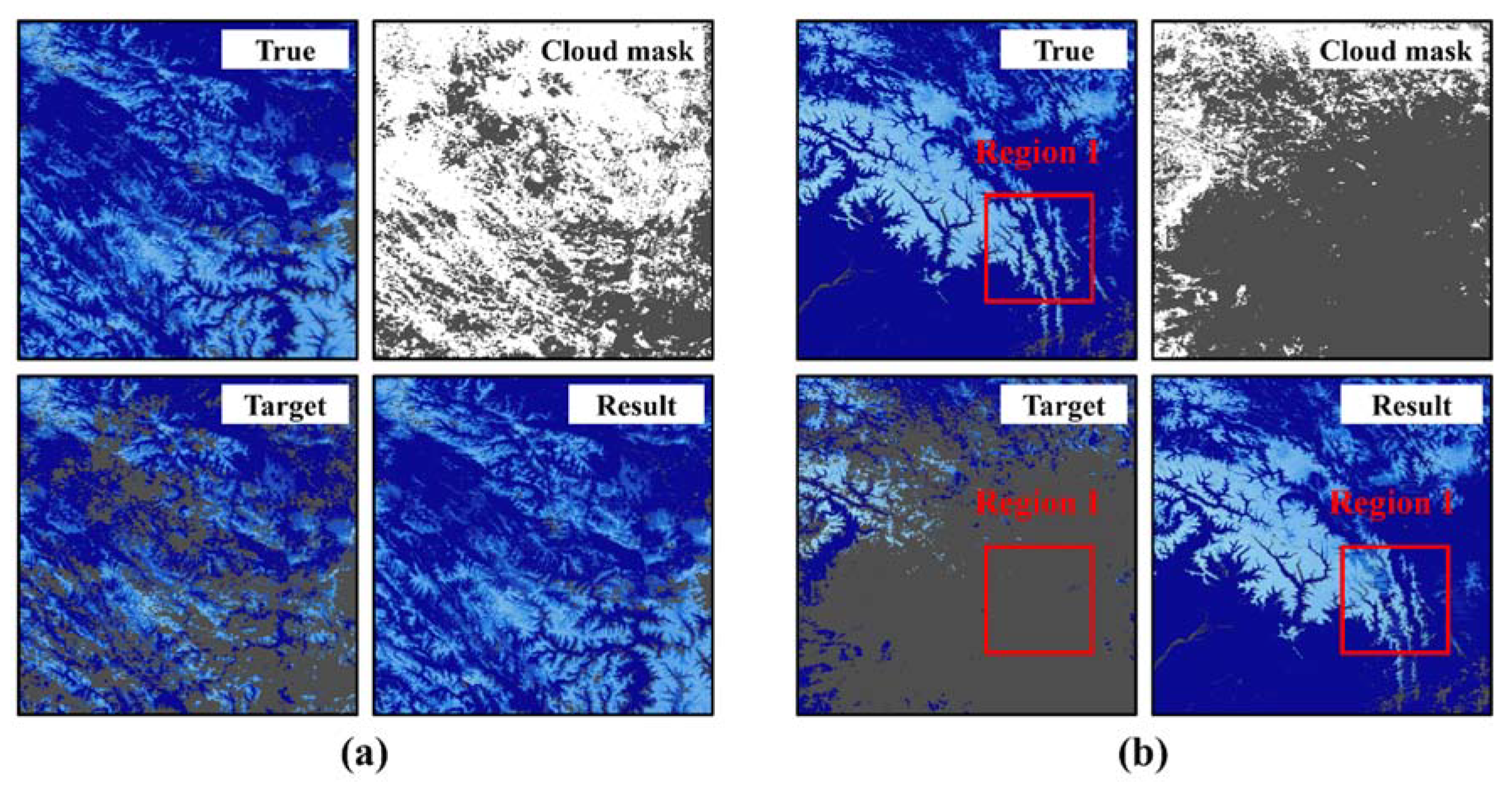
3.3.1. Validation Method Based on a “Cloud Mask Assumption”

Previous studies have typically used snow depth (SD) observations of meteorological stations to estimate cloud removal algorithms for the MODIS binary products; however, this validation method has problems regarding the verification of MODIS NDSI products. First, there is no clear linear relationship between the SD and NDSI [72]; second, the SD of the weather station cannot represent the entire pixel at a scale of 500 m (given the scale mismatch between the weather station and the pixel). Finally, the distribution of meteorological stations across the TP is mostly concentrated in the bottom of the valley at a lower altitude (Figure 1), which is hardly representative of the entire region due to its low spatial density; furthermore, there are no records from certain inaccessible and highly mountainous areas where the snow cover duration is longer. Therefore, another validation method based on a “mask assumption” was adopted in this study. The cloud gaps from other cloudy MODIS NDSI images were used to simulate cloud masks for the “cloud-free” MODIS NDSI image, which is regarded as the true ground information [40,48,73].
The accuracy of the three sub-steps was evaluated independently and sequentially. The cloud removal results of the former method were the input data of the latter method. That is, the input data of the TAC method were the MOD10A1 and MYD10A1, while the output results were the TAC products, which were used as the input products of the 3DTF method. The cloud removal result (3DTF product) of the 3DTF method was used as the input product for the SPSA cloud removal method, and finally, the cloud-free MODIS NDSI product was produced using the SPSA method (Figure 3).
The first two steps (TAC and 3DTF) do not include spatial neighborhood information from cloudy pixels and only consider the temporal information from cloudy pixels. Therefore, their verification method is relatively simple. The specific method is as follows:
(A)
For the TAC method: cloud-free pixels with NDSI values ranging from 0 to 100, both in the MOD10A1 and MYD10A1, were selected as test samples from 2003–2018. Pixels from MOD10A1 were taken as the true values, while the corresponding pixels from the MYD (at the same location) were taken as the predicted value. Equations (7)–(11) express the evaluation indicators.
(B)
For the 3DTF method: from 2003 to 2018, the cloud-free pixels with an NDSI value ranging from 0 to 100 within three consecutive days were selected as test samples, while the observed value of the middle day (date T) was taken as the true value. The arithmetic mean of the previous day’s (date T − 1) NDSI and the latter day’s (date T + 1) NDSI was taken as the predicted value. Equations (7)–(11) express the evaluation index.
It should be noted that the evaluation of these two cloud removal methods (TAC and 3DTF) was performed day-by-day from 2003 to 2018. Each day, all pixels that satisfied these conditions were selected as verification samples. Thus, the accuracy indexes were available for each day.
(C)
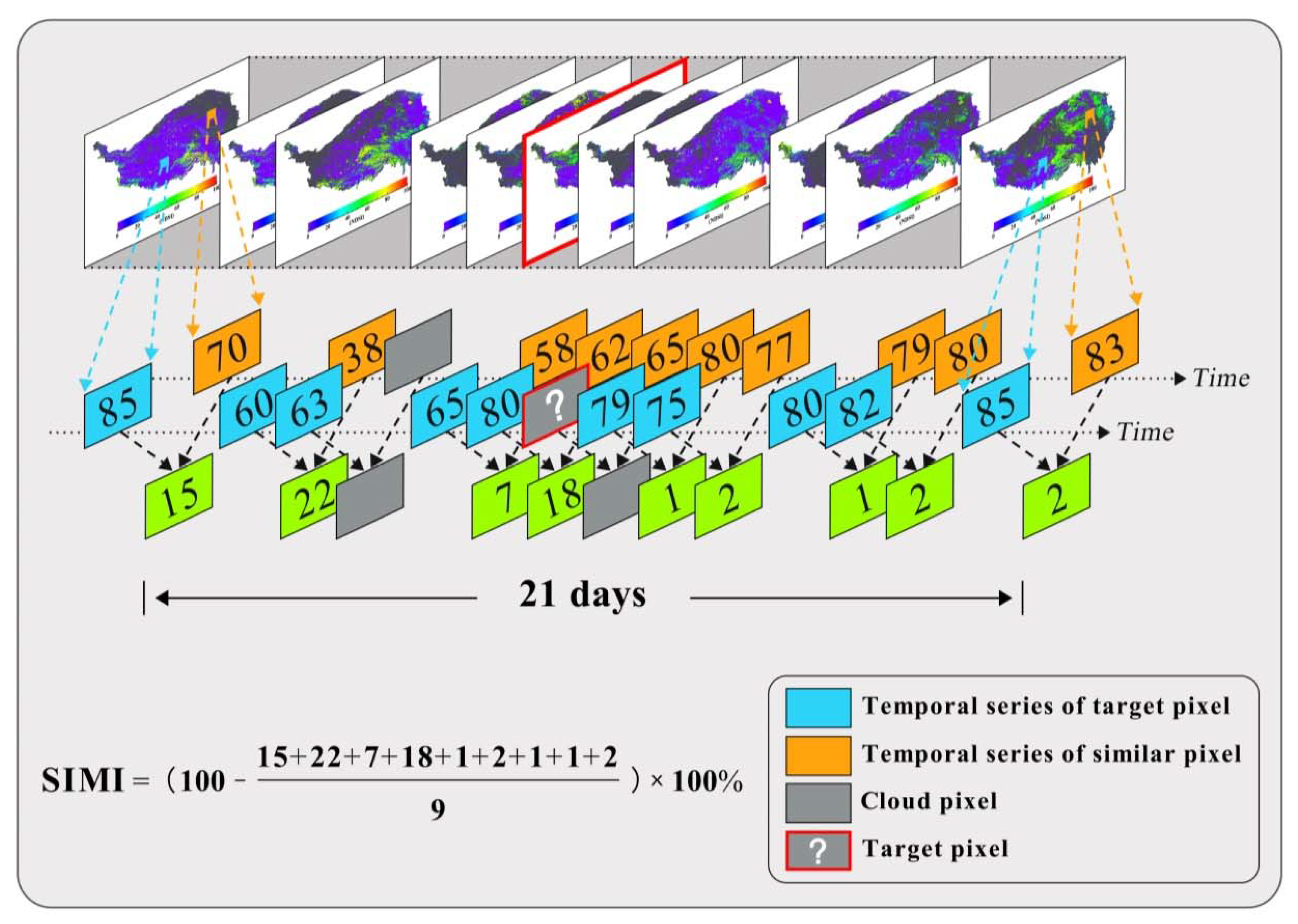
For the SPSA method: a one-day cloud mask assumption was employed for validation. The specific details are outlined below.
The empirical cumulative distribution function (ECDF) [21,30] of the cloud-gap fraction was calculated based on the 3DTF product from 2003 to 2018 and is shown in Figure 6. Cloud contamination with a cloud-gap fraction corresponding to the 25th, 50th, and 75th percentile of the ECDF (hereafter abbreviated as P25, P50, and P75, respectively) are considered low, moderate, and high rates of cloud contamination [30]. The images with a cloud gap fraction closest to P25, P50, and P75 for each month were selected and the corresponding cloud masks were extracted for each month. We then selected three MODIS NDSI images with the lowest cloud-gap fraction for each month from 2003 to 2018 to be designated as “cloud-free” images (i.e., a total of 36 images were selected as “true” images). Each selected “cloud-free” NDSI image was related to three mask images, resulting in a total of 108 validation images from the 16-year study period. The acquisition date, cloud-gap fraction, and snow fraction information from the true images and cloud mask images selected in this study are summarized in Table 1.

3.3.2. Performance Metrics for NDSI

Five performance evaluation criteria (i.e., mean error (ME), mean absolute error (MAE), mean absolute percentage error (MAPE), root mean square error (RMSE), and the coefficient of determination (R2)) were employed and calculated using the following equations:
M E = 1 N i = 1 N ( x i P r e d i c t e d x i O b s e r v e d ) ,
M A E = 1 N i = 1 N A B S ( x i P r e d i c t e d x i O b s e r v e d ) ,
M A P E = 1 N i = 1 N A B S ( x i P r e d i c t e d x i O b s e r v e d ) ÷   x O b s e r v e d ¯ × 100 % ,
R M S E = 1 N i = 1 N ( x i P r e d i c t e d x i O b s e r v e d ) 2 ,
R 2 = ( 1 N 1 i = 1 N ( x i P r e d i c t e d x P r e d i c t e d ¯ σ P r e d i c t e d ) ( x i O b s e r v e d x O b s e r v e d ¯ σ O b s e r v e d ) ) 2 ,
where x i P r e d i c t e d is the estimated NDSI value of the ith cloud mask pixel, x i O b s e r v e d is the corresponding true NDSI value, N is the total number of cloud mask pixels, and σ P r e d i c t e d and σ O b s e r v e d denote the standard deviations of the estimated and true NDSI value, respectively.

3.3.3. Classification Accuracy

Binary snow cover products (snow-covered or snow-free) are still widely used in water cycles, global climate change, water and heat energy balances, and other research fields. NDSI products can be converted into binary snow cover products according to specific thresholds [51], and thus, they serve as input parameters for numerous hydrological and climate models. To evaluate the accuracy of cloud-free NDSI products obtained by the proposed cloud removal algorithm when converted into binary snow cover products, the confusion [74] matrix method (Table 2), which is recommended by several studies [14,32,35,75,76], was used in this study to evaluate the classification accuracy of different cloud removal algorithms. The threshold for the binary classification used in this study was 40, which is recommended by the MODIS standard snow cover product.
Three validation indices are defined as follows:
O A = ( s s + n n ) ( s s + s n + n s + n n ) × 100 % ,
O E = n s ( s s + s n + n s + n n ) × 100 % ,
U E = s n ( s s + s n + n s + n n ) × 100 % ,
where the overall accuracy (OA) is the probability that a MODIS pixel is correctly classified as snow or snow-free; UE and OE represent the underestimation and overestimation snow error, respectively. A perfect estimation of MODIS gives OA = 1, and OE = UE = 0. A completely failed estimation of MODIS is OA = 0, and UE + OE = 1 [30].

4. Results

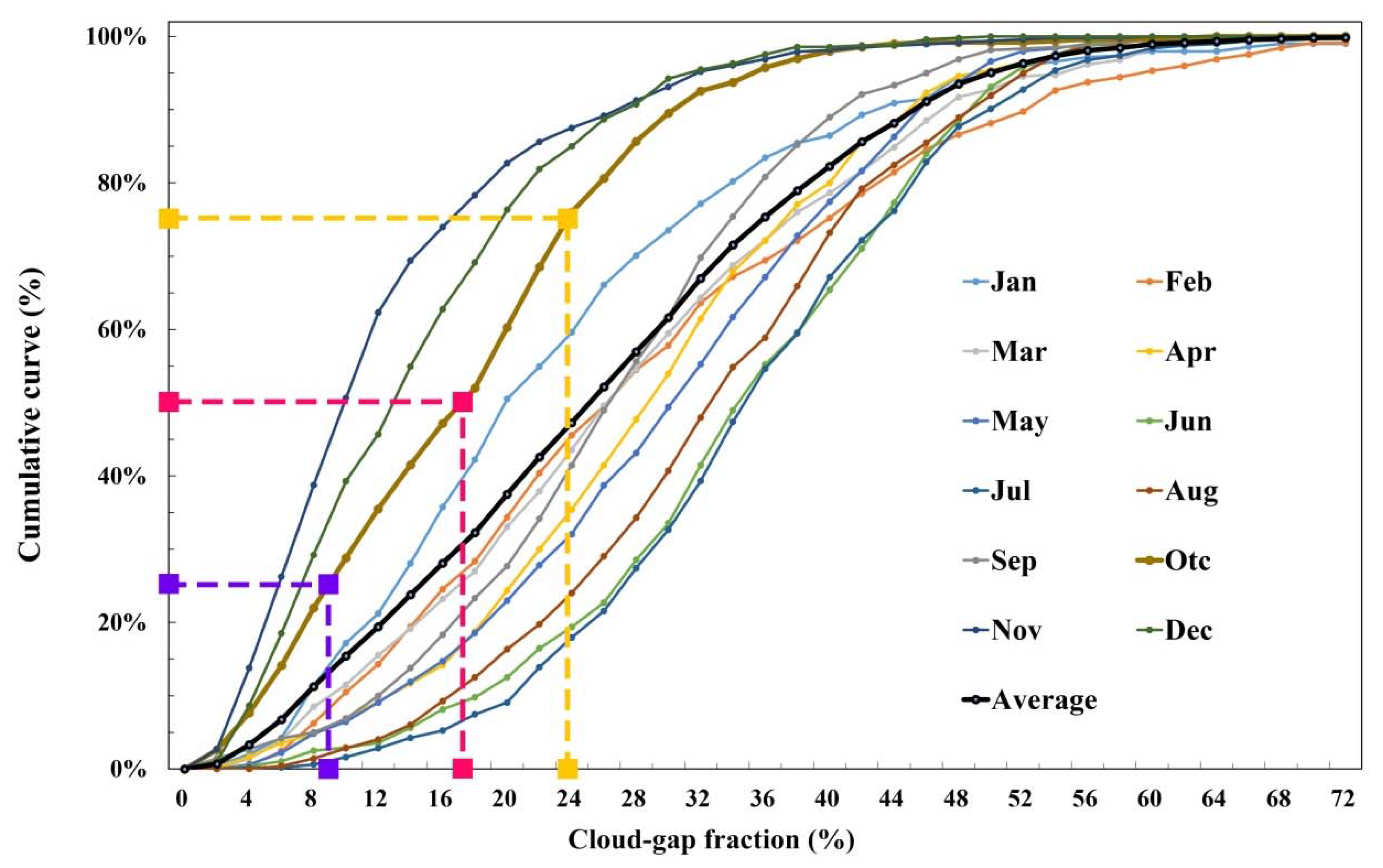
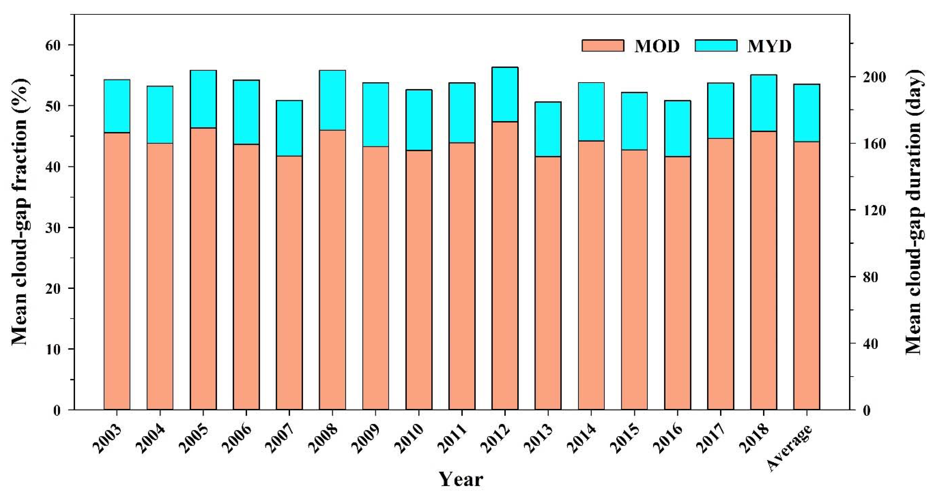
4.1. Cloud Gaps in MODIS NDSI Products across the TP

An understanding of the spatial and temporal distribution characteristics of clouds across the TP is the basis and premise for selecting an appropriate and effective cloud removal method [30]. After investigating the cloud gaps in the MODIS NDSI products of the TP, we found that the annual average cloud-gap fraction of the study area was 41.62–47.38% for Terra and 50.61–56.32% for Aqua from 2003 to 2018, with mean cloud-gap fractions of 44.06% and 53.55%, respectively (Figure 7). The results show that the mean number of cloudy days was 151–172 days for MODIS Terra NDIS images and 184–206 days for MODIS Aqua NDSI images, with means of 161 and 195 cloudy days, respectively (Figure 7 and Figure 8). Although there were slight differences in the extent and duration of cloud contamination from year to year, the spatial distribution and pattern of cloud coverage from year to year across the TP seemed relatively stable.
Overall, the MYD10A1 (obtained from Aqua at 13:30) had approximately 9% more cloud coverage than MOD10A1 (obtained from Terra at 10:30). This may have resulted from temperature increases, vegetation transpiration, and increases in soil evaporation throughout each day, which created conditions that favored cloud formation. The distribution of cloud contamination across the TP was very uneven, with high values mainly concentrated on the southeastern part of the TP, especially in the Hengduan mountain regions. The annual average cloud cover duration of these areas exceeds 250 days, making cloud removal very challenging.
MODIS Terra NDSI products were taken as an example to further analyze the relationship between cloud coverage and time. The monthly average cloud coverages in different elevation zones are shown in Figure 9. Based on Figure 9, the monthly multi-year average cloud coverage for each elevation zone demonstrated that the proportion of cloud cover in the TP changed with time, which occurred as follows: all areas (except for areas with altitudes above 6000 m) showed a similar seasonal cycle, reaching their maximum values in summer (June, July, and August), and had an average cloud cover of 54.1% (for all areas except the areas above 6000 m). When autumn arrived, the cloud coverage began to decline rapidly from September and reached the minimum value in November (with a mean value of 25.7%). Winter and the following spring showed a gradually increasing trend. The opposite trend was observed for areas over 6000 m.a.s.l. Cloud coverage peaks in the winter were as high as 80% in January, and were relatively low in the summer, at approximately 40%. This may have been due to MODIS misinterpreting the snow cover as clouds at high altitudes [77].
Despite the high cloud cover over the TP, most of the cloud cover was concentrated in the summer months. This was beneficial for cloud removal in snow products, as previous studies [33,34] indicate that, in the summer, when the temperature is at its highest, the remaining snow can be considered permanent snow cover, which only exists on the peaks of the highest mountains. This type of snow can be considered perennial (i.e., there is always snow under the cloud cover). This significantly reduces the need for cloud removal in binary snow products [33,34]. In autumn and spring, when the snow cover was sensitive to global climate change, cloud cover was relatively low, which facilitated the cloud removal procedure.

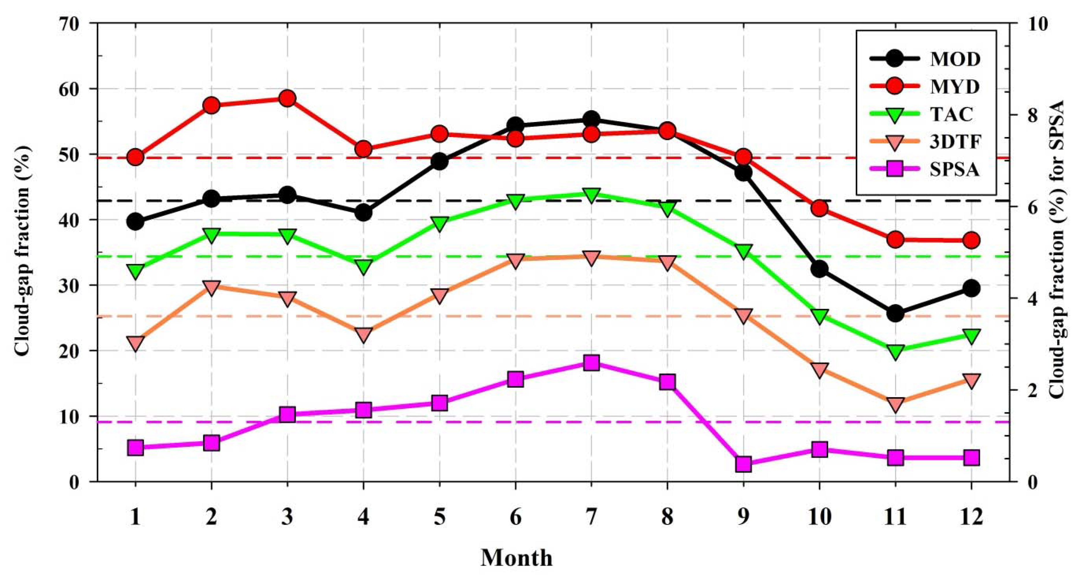
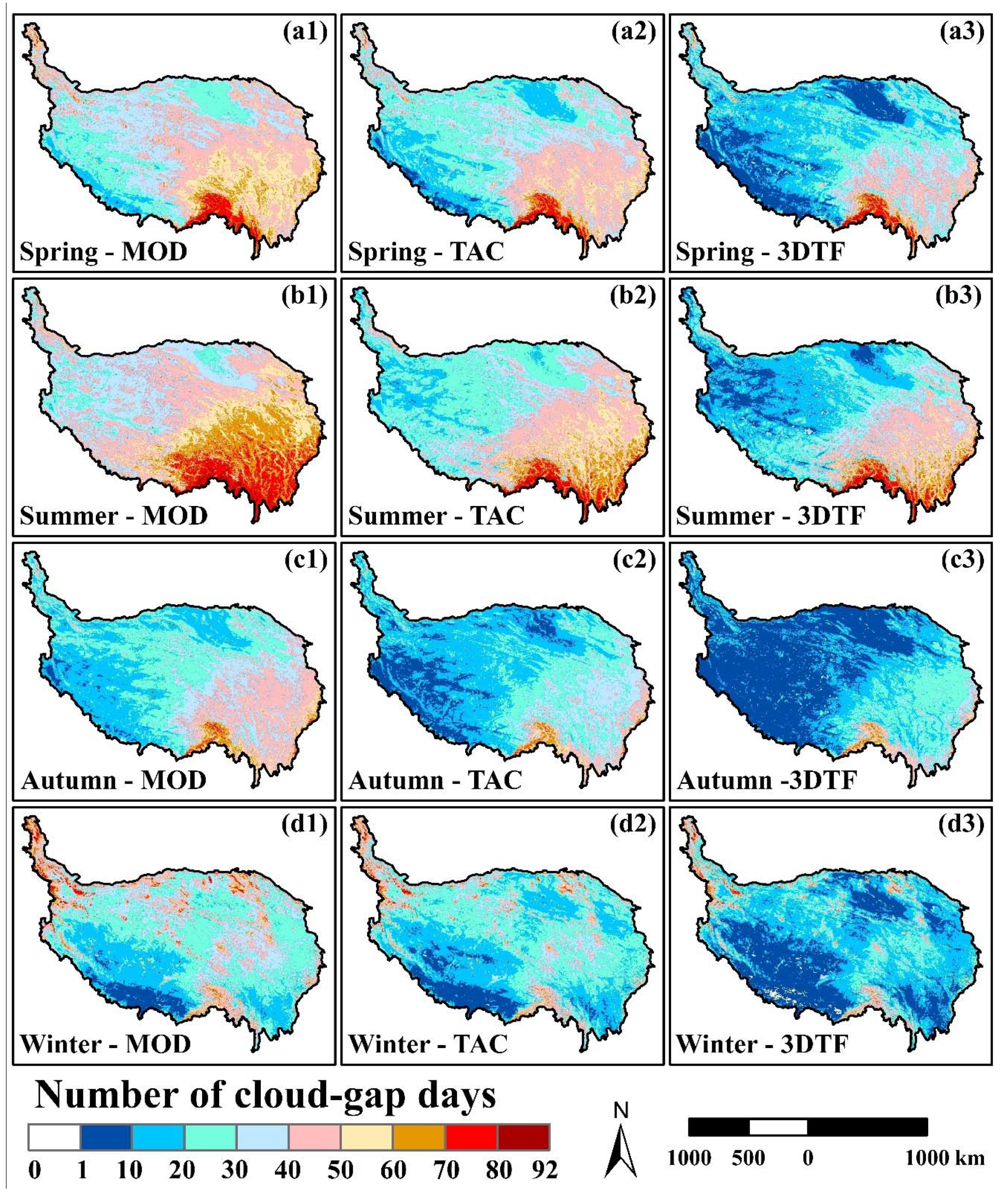
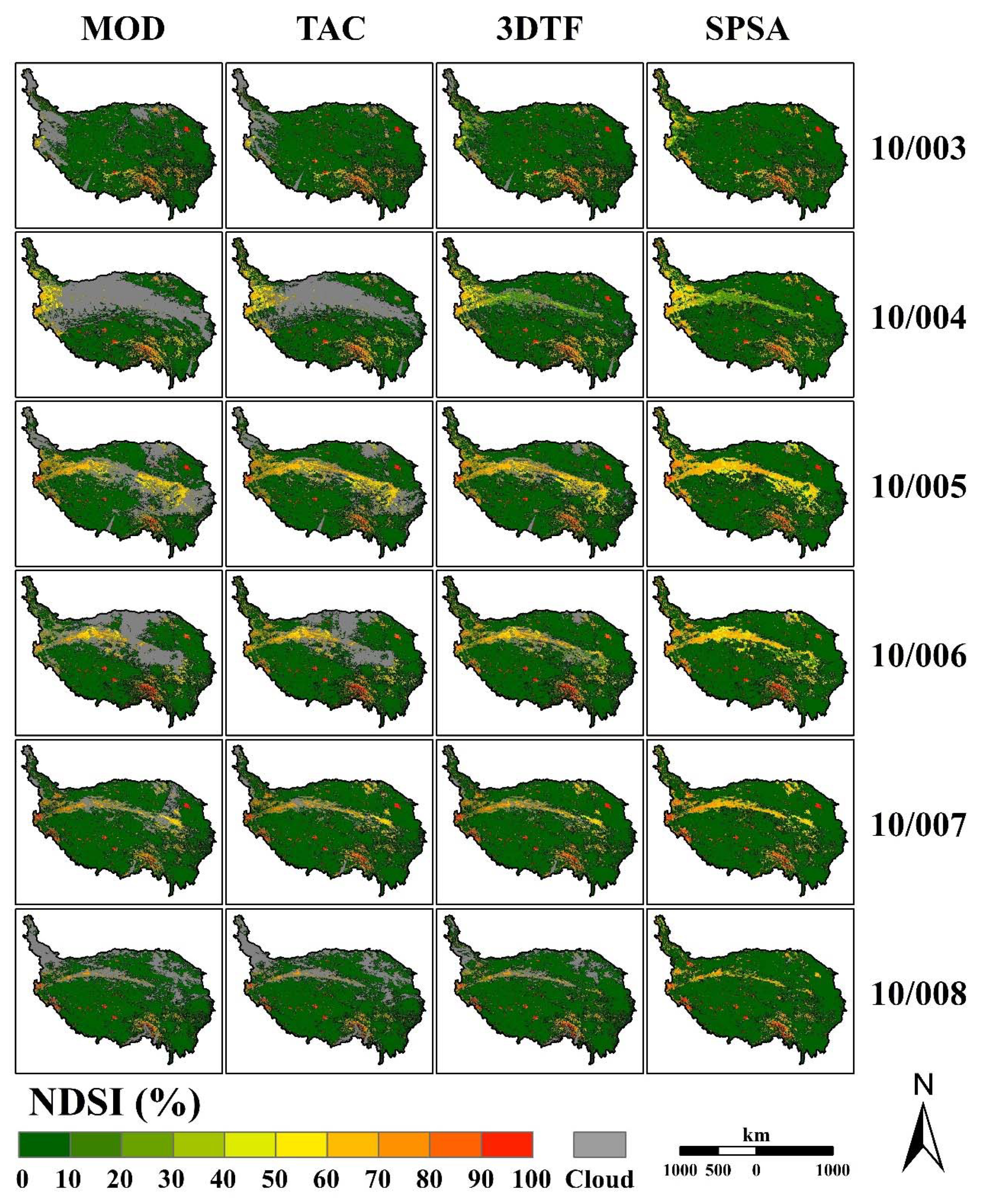
4.2. Effectiveness of the Gap-Filling Methodology

Figure 10 presents the mean cloud-gap fraction in different months after the execution of each gap-filling step. The TAC and 3DTF reduced the cloud gaps by an average of 8.19% (compared to the original Terra data) and 9.43%, respectively. The SPSA method removed the remaining ≈25% of cloud gaps, leaving only less than 1.5% on average.
Figure 11 illustrates the spatial distribution of the average number of cloud-gap days (CGDs) for the MOD, TAC, and 3DTF products at a seasonal scale. The results indicate that the cloud occlusion in the TP was significantly mitigated by the TAC and 3DTF methods. The TAC algorithm reduced the number of the CGDs for the MOD products from 41.9, 49.0, 30.6, and 31.8 days to 35.3, 38.8, 23.5, and 26.6 days, for spring, summer, autumn, and winter, respectively. Moreover, the 3DTF algorithm further reduced these values to 26.1, 30.6, 16.2, and 19.3 days, respectively. For the 3DTF product, the areas with CGDs below 30 days in the autumn and winter accounted for 88.9% and 84.1% of the total area of the TP, respectively, which suggests a relatively small need for cloud removal in autumn and winter. During the spring and summer, areas with more than 60 days of CGD accounted for 3.4% and 6.9% of the entire TP. This part of the region presented the most difficulties for cloud removal via the SPSA method due to a lack of effective temporal information.
Figure 12 shows a time-series example of cloud-free NDSI distribution maps after the TAC, 3DTF, and SPSA gap-filling steps. The remaining cloud-gapped fraction decreased to less than 1% after the multi-step cloud removal procedure. Figure 12 displays a complete snowfall and snowmelt dynamic process. From 3 January 2010, it first began to snow in western TP. Over the next few days, with the movement of the weather system, the snow rapidly spread across the eastern part of the Tibetan plateau, reaching the maximum snow-covered area on 5 January. Over the next four days, the snow melted rapidly. The entire process of snowfall and melting occurred very rapidly, in less than a week, which reflected the rapid changes in the characteristics of the TP snow state.

4.3. Accuracy Assessment

4.3.1. Accuracy Assessment of the Terra and Aqua Combination (TAC) Method

Figure 13 illustrates the performance metrics for NDSI and the classification accuracy of the TAC filter.
Based on Figure 13a, the MAE and RMSE had a similar seasonal cycle. Figure 13a shows that the low value of the MAE and RMSE occurred in winter (December, January, and February) and summer (June, July, and August), with MAE = 2.57 and RMSE = 3.77 for winter and MAE = 2.45 and RMSE = 3.41 for summer. The high value occurred in the spring (March, April, and May) and autumn (September, October, and November), with MAE = 3.38 and RMSE = 4.28 for spring and MAE = 2.86 and RMSE = 3.81 for autumn. MAE (or RMSE) was lower in winter because the temperature was at its lowest in the year, such that it was easy to preserve the snow cover and the snow cover state did not change easily. Therefore, the observed values for the MOD (crossing at 10:30) and MYD (crossing at 13:30) are relatively close. The reason for the low MAE (or RMSE) in summer was that the snow cover on the TP only appeared in high-altitude areas of the highest mountains in the summer. The average NDSI of the entire TP was the minimum NDSI of the entire year, such that the MAE (or RMSE) was also relatively low.
Spring, however, was the season in which snow began to melt. With the gradual increase in temperature, the snow status changed rapidly, such that the observed values of MOD (crossing at 10:30) and MYD (crossing at 13:30) could change due to temperature and solar radiation. MAE (or RMSE) also showed a trend that first increased and then decreased in the spring. R2 was lower from June to September, averaging only 0.52, while the annual average R2 was 0.67.
The classification accuracy and performance metrics for NDSI had similar characteristics (Figure 13). The lowest value of the overall accuracy appeared in the spring (OA = 96%), followed by autumn (OA = 97%). High values for the OA occurred in winter (OA = 98.1%) and summer (OA = 98.2%). The error in the OA was mainly derived from the UE. The UE showed a significant trend over time, with high values appearing in spring (UE = 3.2%) and autumn (UE = 2.6%). The reason for this could be that the NDSI values observed by the MYD were lower than those observed by the MOD due to the snow melting caused by the temperature rise at noon. This phenomenon was most evident in the spring.
Overall, the NDSI values observed using MOD and MYD had a good consistency, with an annual average MAE of 2.82. In winter, the consistency was higher, with an MAE of only 2.57. In spring and autumn, the MAE values were 3.38 and 2.86, respectively. This indicates that the overall de-clouding accuracy of the MOD and MYD fusion method was high, and therefore, this method can be employed for cloud removal.

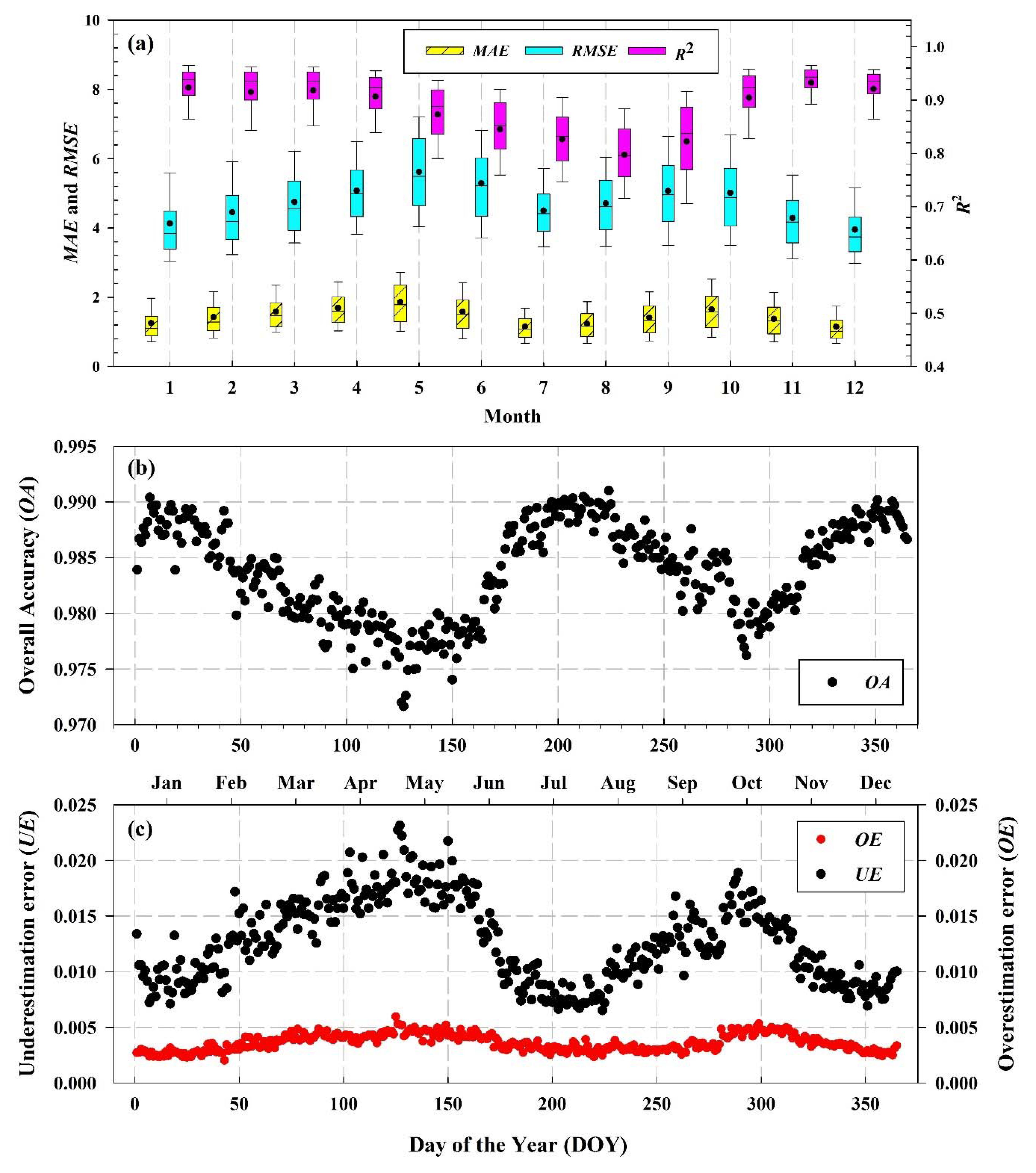
4.3.2. Accuracy Assessment of the Three-Day Temporal Filter (3DTF) Method

Figure 14 illustrates the performance metrics for NDSI and the classification accuracy of the 3DTF. Both the OA and UE changed with time (season), while the OE showed a relatively insignificant change with time. The OA was the lowest in spring and autumn (97.2% and 97.6%, respectively) and the highest in winter and summer (both exceeding 99%). The annual OE was maintained at a very low level (only 0.5%) and depended weakly on time. This indicates that the decrease in the OA was mainly due to the contribution of the UE, which was also consistent with the findings demonstrated in Figure 14. The annual average OA was high, reaching 98%; the annual average value of the UE was 2%, which was greater than that of the OE (0.5%).
The error associated with the 3DTF method mainly derives from the UE, where the peak UE value appeared in the spring and autumn, which was consistent with the snow cover characteristics of the TP. The snow layer on the TP was thin, the snow patch was relatively broken, the solar radiation was strong, the wind speed was high, sublimation was common, and the snow state changed rapidly. As the snow depth was shallow and the snow episodes were short, the snow cover that accumulated in the morning of date T may have melted in the afternoon of the same date or at date T + 1. In other words, in such a scenario, the NDSI of date T − 1 was zero (the accumulation of snow had not yet begun), the NDSI of date T was high (snow began to accumulate on date T), and the NDSI of date T + 1 was low (snow cover began to melt). In this case, the 3DTF method underestimated the NDSI value. Moreover, this phenomenon was more common in snow-accumulation (autumn) and snow-melting periods (spring). On the other hand, in winter, due to the low temperature, the snow cover state was more likely to be consistent, such that the UE was low. The reason for the low UE in summer was that the snow cover was only distributed on the highest mountains of the TP in summer. The snow cover is generally considered to be permanent snow cover, which is in a relatively stable state. Therefore, the UE in summer was low and the OA was high.
In general, the accuracy of the 3DTF method was very high. The annual average OA reached 98% but the accuracy varied with time. The OA was high in stable periods (winter and summer) but relatively low in the snow-accumulation (autumn) and snow-melting periods (spring).

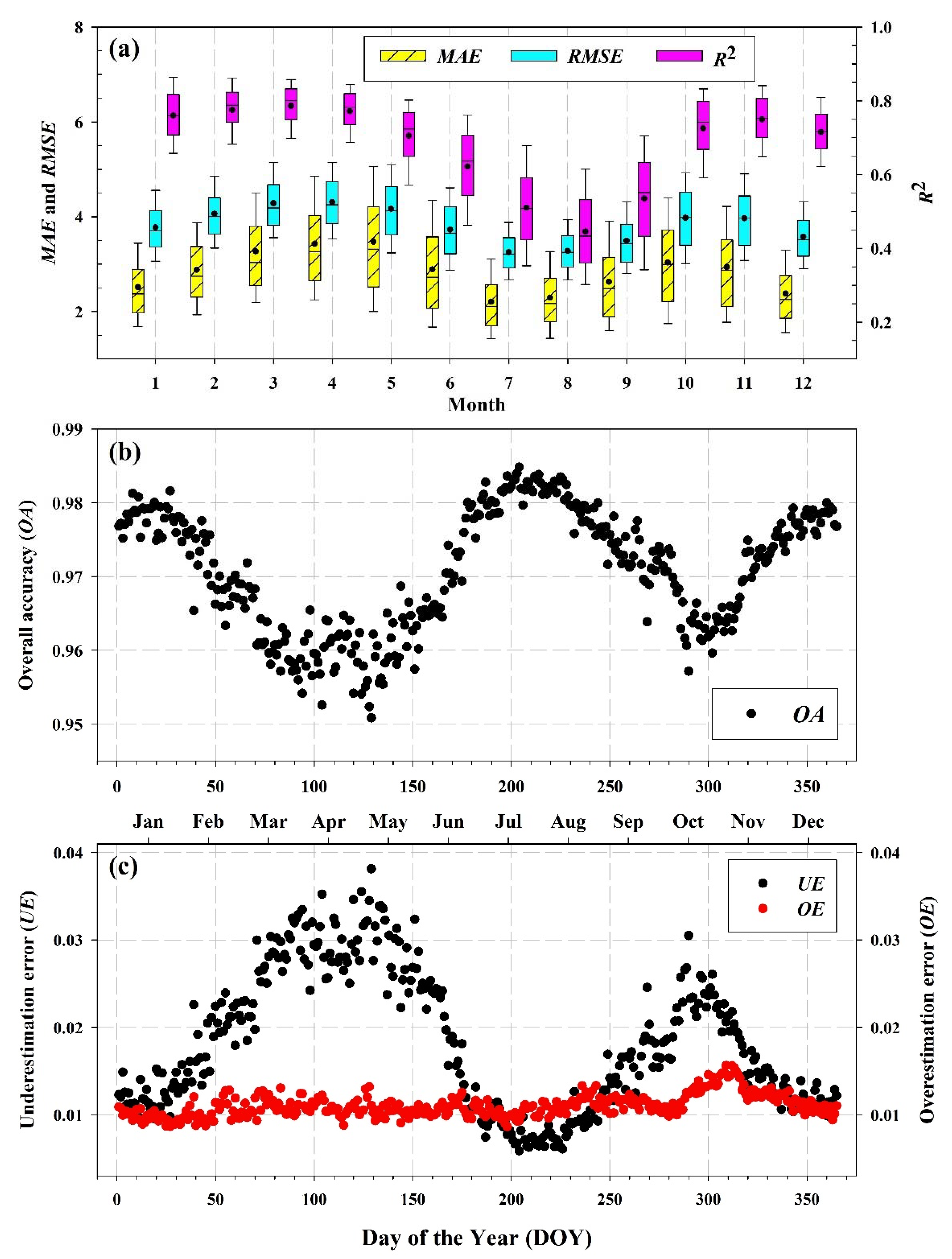
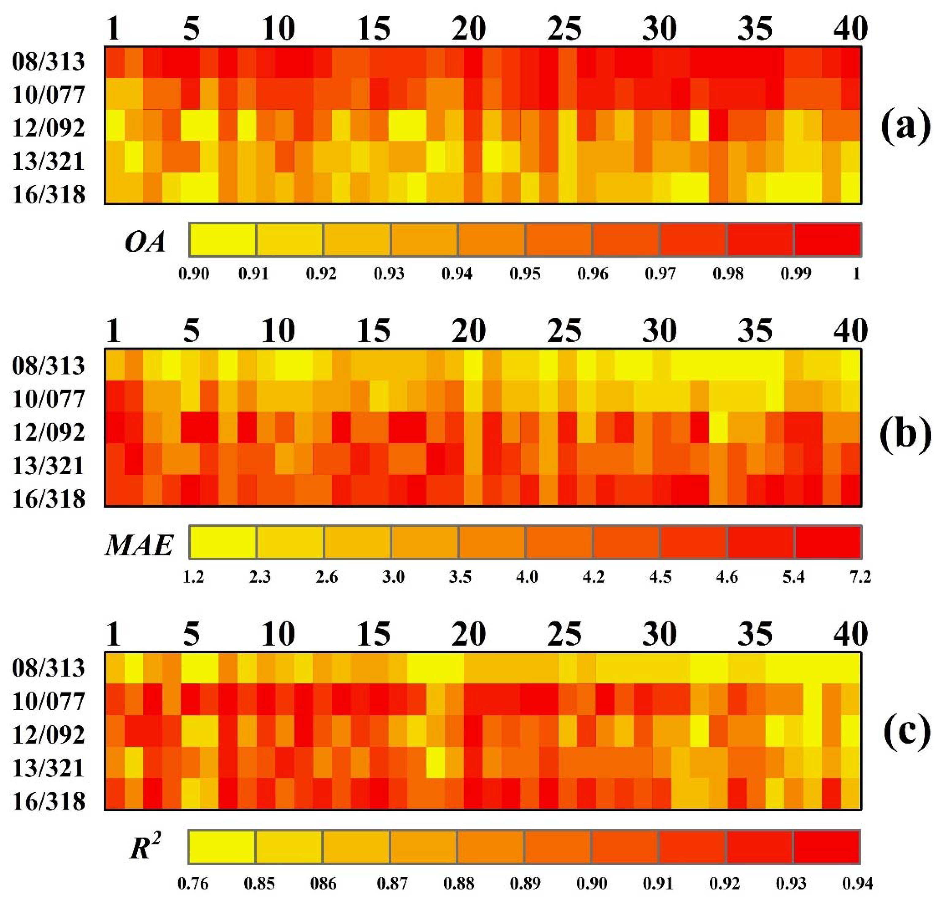
4.3.3. Accuracy Assessment of the Similar Pixel Selecting Algorithm (SPSA)

According to the validation method introduced previously, the cloud removal experiment was conducted on 108 samples, and the performance of the SPSA algorithm was evaluated regarding the two aspects of performance metrics for NDSI and classification accuracy (Table 3). Overall, the accuracy of the SPSA algorithm was high. In terms of the performance metrics for NDSI, the annual averages were as follows: MAE was 2.77, RMSE was 3.78, and R2 was 0.78. In terms of the classification accuracy, the annual average OA was 96.92%, the OE was quite low at only 1.10%, and the UE was greater than the OE at 1.98%. Therefore, it can be inferred that the main error source of the SPSA algorithm was the UE.
The performance of the SPSA algorithm was different for the four seasons (Table 3), among which, the accuracies for autumn, winter, and spring were close, whereas the situation in summer was unique. Among autumn, winter, and spring, autumn had the highest accuracy, followed by spring and winter. It is worth noting that, although the absolute indicators (i.e., the MAE, RMSE, and OA) in autumn were better than those in winter and spring, the relative indicators (MAPE) in autumn were slightly higher than those in winter and spring at 37.84%. This was mainly due to less snow cover in autumn compared with winter and spring, such that the relative error was larger.
Summer had the lowest MAE (1.69) and RMSE (2.86) of the year and the highest overall accuracy (OA = 98.54%) for the whole year, but its relative error was the worst (MAPE = 71.12%). The R2 was also the lowest for the whole year at only 0.62. Therefore, a high summer accuracy (low MAE and RMSE, high OA) was considered to be a “false high precision.” The reason for this “false high precision” was that there was less snow cover in the summer and more snow-free areas. Even if the snow was misclassified in snowy areas, it accounted for only a small portion of the total, such that the OA was still high. The SPSA algorithm for summer was limited as summer was the season with the highest number of days covered by clouds in a year (Figure 11(b3)), i.e., the number of days covered by clouds in certain pixels during summer was nearly 80 days. These pixels did not provide valid temporal information. There was little temporal information available during the similarity pixel calculation, such that there was a reduction of the accuracy in the SPSA algorithm (R2 was only 0.62). However, summer snow usually exists only in the high-altitude mountains, which is considered permanent snow [33,34]. The snow state is relatively stable, such that the remaining clouds in summer can be removed by other methods [33,34].
Figure 15 details the SPSA algorithm. The date associated with the data was 08/010, with an image size of 400 × 400 pixels (approximately 40000 km2) (a) and 600 × 600 pixels (approximately 90,000 km2) (b). Based on Figure 15, the SPSA algorithm could remove almost all cloud contamination. From a visual perspective, the SPSA algorithm could restore the missing snow information beneath the cloud, rendering the predicted snow distribution pattern highly consistent with the observed snow distribution pattern. However, the SPSA algorithm also had certain missing points. The omission areas were mostly concentrated in the transition area between snow and land, but not in the center of large areas covered with snow. We speculate that the reason for this was a relatively thin snow layer in this part of the snow–land boundary, as well as rapid changes in the snow state, particularly with newly fallen thin snow, which melted within a short period. Therefore, the information provided in the time dimension (both before and after the snow) had a lower NDSI value, such that the selection of a similar pixel introduced error. This was also consistent with the conclusion listed in Table 3, i.e., the UE of the SPSA algorithm was approximately twice the OE. The SPSA algorithm performed well for large cloud areas (Figure 15b). Even when the cloud coverage exceeded 75%, the missing NDSI value could be reconstructed. However, certain errors were identified within large cloud patches, such as region I in Figure 15b. This may have been due to the large size of the cloud patch areas, which increased the distance between the target pixel and similar eligible pixels, thus reducing the accuracy of the algorithm.

5. Discussion

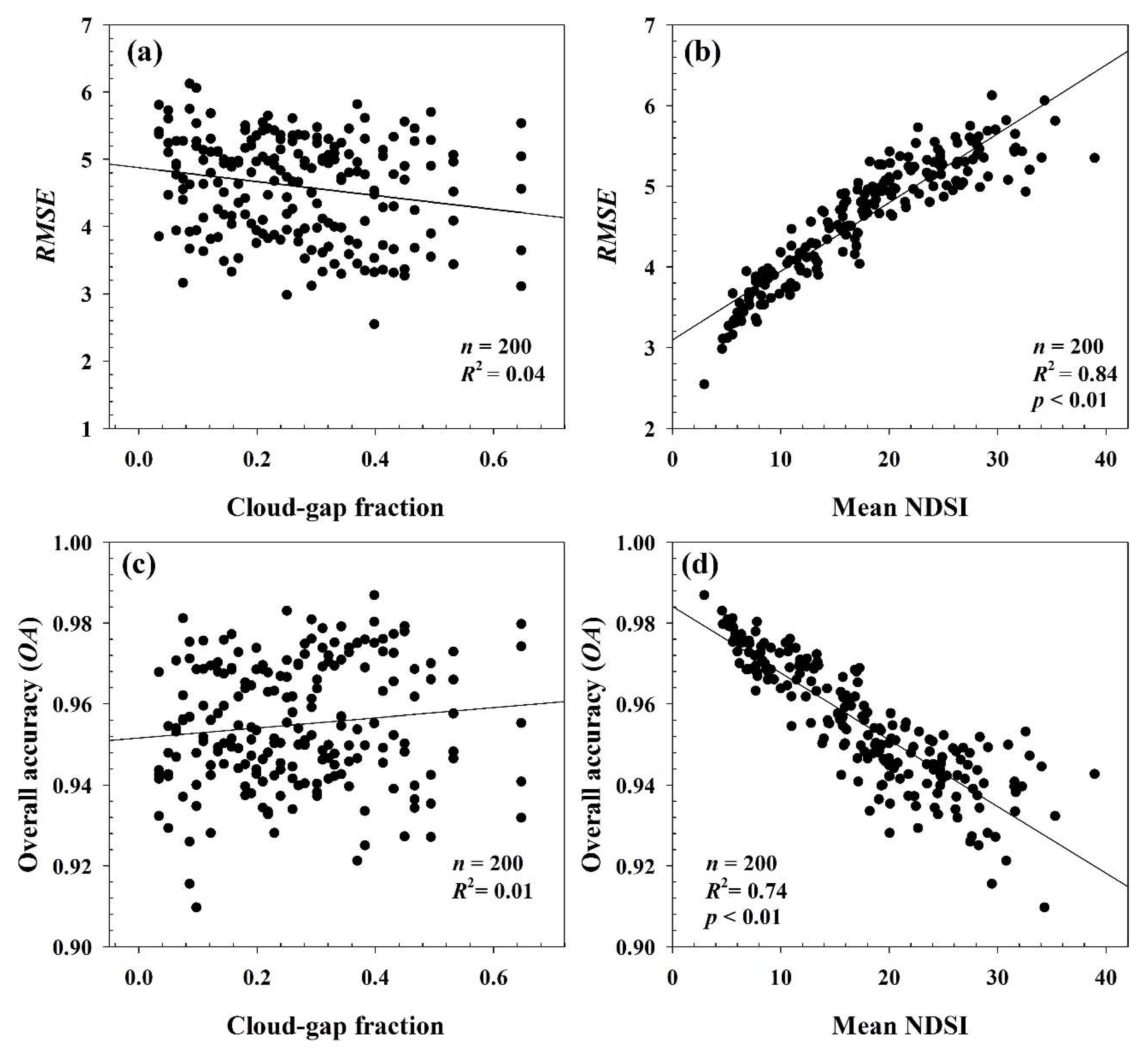
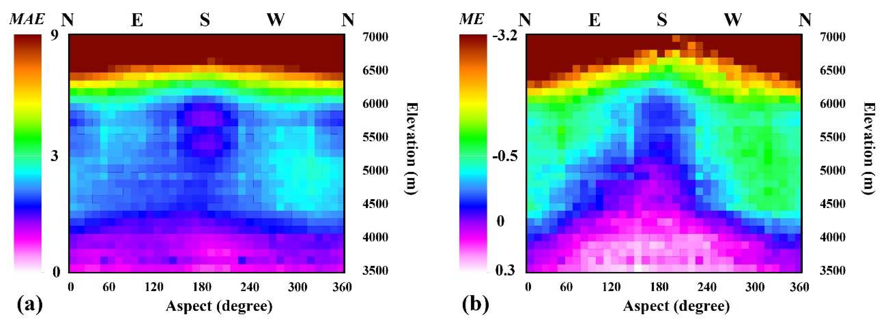
5.1. Impact Factor Analysis of the SPSA Algorithm

To further analyze the relationship between the accuracy of the SPSA algorithm and the cloud occlusion rate, we randomly selected five images with a cloud-gap fraction of less than 3%: 08/313 (CGF = 1.69%), 10/077 (CGF = 2.18%), 12/092 (CGF = 2.26%), 13/321 (CGF = 2.86%), and 16/318 (CGF = 1.61%). According to the cumulative frequency of the cloud-gap fraction for the 3DTF product (Figure 6), the cloud mask images were selected according to the proportion of the annual mean cloud-gap fraction from small to large. A total of 40 cloud mask images were selected. Table 4 lists the dates of the true and cloud mask image and the cloud fraction. For each true image scene, 40 cloud masks with a different cloud-gap fraction (from 3.42% to 64.68%) were employed. Thus, a total of 200 combinations were validated. The accuracy of the SPSA algorithm was then evaluated according to the previously mentioned cloud mask assumption method.
Figure 16 shows the accuracy indexes. In general, with these 200 images as verification samples, the average MAE of the SPSA cloud removal method was 3.78, the average RMSE was 4.60, the average R2 was 0.88, and the average OA was 95.49%, which was consistent with the previous results in this study.
Subsequently, we calculated the relationship between the accuracy of these 200 groups of samples (RMSE and OA were selected as evaluation indicators), the cloud-gap fraction, and the mean NDSI of all pixels under the cloud (mean NDSI of all cloudy pixels).
Figure 17 shows the scatterplots of the relationships among the various accuracy indexes. The results show that the accuracy of the SPSA cloud removal method (RMSE and OA) was independent of the cloud-gap fraction (R2 = 0.04 for RMSE and 0.01 for OA). However, both the RMSE and OA had a strong correlation with the average mean NDSI value of the pixels under the cloud (R2 = 0.84 and 0.74, respectively). The RMSE was positively correlated with the mean NDSI of the cloudy pixels, while the OA exhibited a negative correlation.
We then further analyzed the prediction results of 108 scene verification datasets used in Section 3.3.1 according to the zoning of elevation and aspect. The relationship between accuracy and topographical factors (elevation and aspect) also provided indirect evidence for our conclusions. Figure 18 demonstrates the accuracy’s changing pattern with elevation and aspect. Accuracy generally decreased with increasing elevation. Aspect also affected the accuracy of the SPSA algorithm (Figure 18). Specifically, the error associated with the sunny slope was small, while that of the shaded slope was large. This effect was especially notable between 4000 and 6000 m above sea level, but not below 4000 m or above 6500 m. Low areas (<4500 m) exhibited an overestimation and high areas (>4500 m) an underestimation (Figure 18b).
Previous studies have demonstrated a relationship between snow cover and elevation, which generally indicates that snow cover duration increases with elevation [6,62,78,79,80,81]. Moreover, snow cover duration is lower in sunny slopes relative to shaded slopes due to solar irradiation [78,80]. The absolute accuracy of the SPSA algorithm can also be attributed to the consistent spatial distribution of snow, which is consistent with our previous observations.
This result shows that the accuracy of the proposed method was not affected by the cloud-gap fraction and had a good robustness under different cloud cover circumstances. However, the NDSI itself affected the accuracy. If the mean NDSI value of cloudy pixels was large, cloud removal was more difficult, such that there was a reduction in the accuracy. When the mean NDSI was small (e.g., clouds were above snowless areas), cloud removal was much easier.

5.2. Comparison between TAC, 3DTF, and SPSA

Previous studies have demonstrated the satisfactory accuracy of existing MODIS cloud gap-filling methods during the stable-snow-cover phase, but these approaches cannot achieve acceptable accuracies in the transition phase characterized by snow cover accumulation and ablation [23,47]. Compared with the TAC and 3DTF methods, the SPSA algorithm showed no significant difference in accuracy during the stable snow-packed phase (winter) and snow-transition phase (spring and autumn) (Table 5). The accuracies during autumn and spring (snow-cover accumulation and ablation phase) were not lower than that of winter (snow-packed phase), but slightly higher, which suggests that the SPSA method was also effective during the snow transition period. This may have been because cloud coverage reached a minimum in autumn, during which, time-series information was more abundant, thus facilitating the accurate selection of similar pixels.
The TAC and 3DTF algorithms are widely used in numerous cloud removal algorithms. Typically, these two algorithms are implemented first, followed by other algorithms. However, there are relatively few studies on accuracy evaluations for these two methods. This study demonstrated that both the TAC and the 3DTF methods had high accuracies, which could provide a theoretical basis for future studies. The SPSA algorithm could eliminate the remaining ≈25% cloud gaps without a significant loss of accuracy, which was the value of the SPSA algorithm. When using the proposed cloud removal method, users can specify how to combine the three algorithms according to their requirements. Additionally, the SPSA method can be used independently.

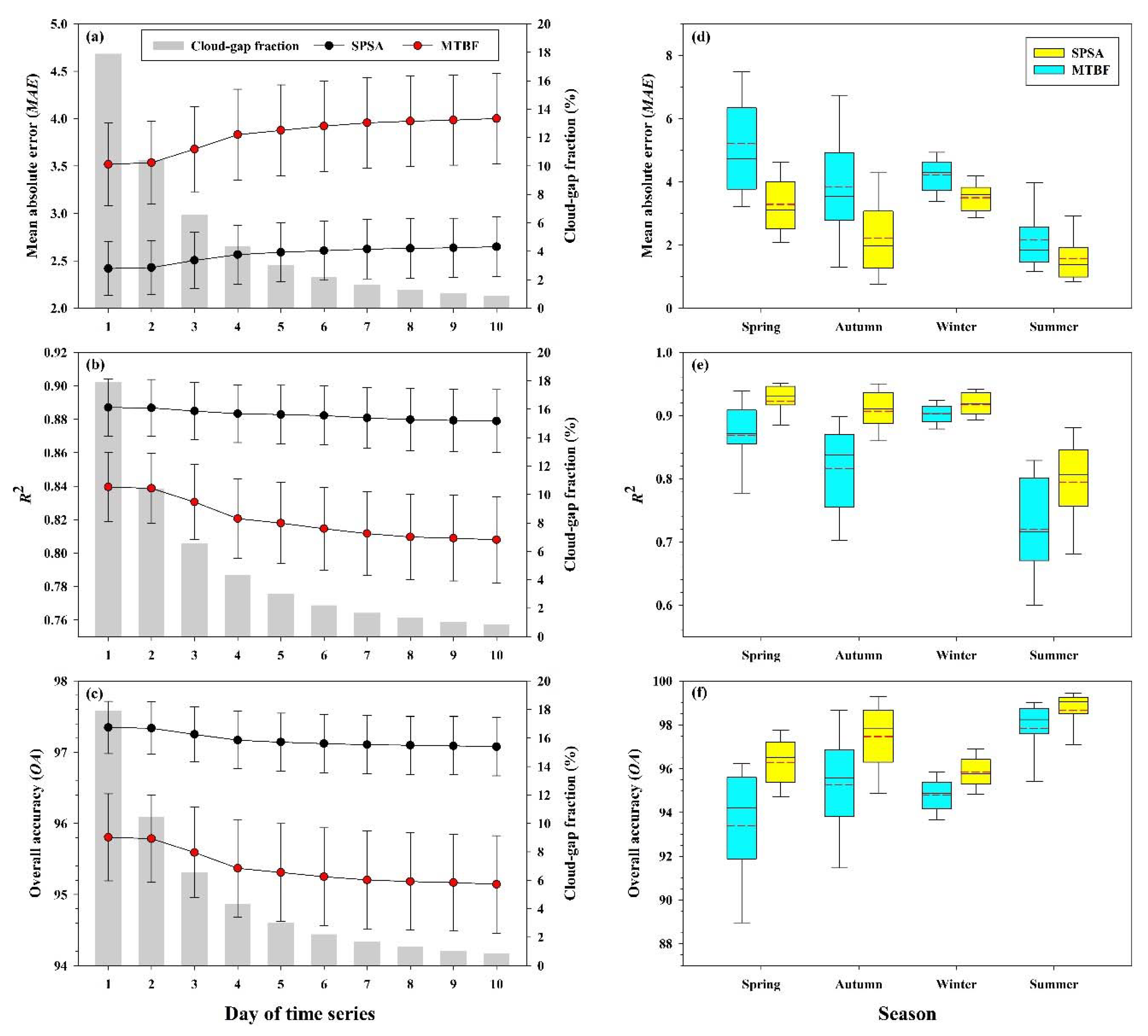
5.3. Comparison between SPSA and the Multi-Temporal Backward Filter

The multi-temporal backward filter (MTBF) has been successfully used by numerous studies with the MODIS standard snow products and other satellite data [40,58]. Using the MTBF, Hall et al. [82] generated cloud-gap filled daily snow cover extent map products. The cloud pixels on the current day of M*D10A1 were replaced with the most recent previous cloud-free pixels (snow/snow-free) from the M*D10A1 (see Hall and colleagues [82,83] for details). The method proposed in Hall et al. [82] is the method that was selected for the NASA MODIS standard snow cover extent (SCE) products because of its ease of use and effectiveness, as well as due to its reliance on data from only one sensor at a time to produce the results [83]. This method can also be employed for MODIS NDSI products [83].
We compared the performance of the SPSA and MTBF algorithms. The input data was the 3DTF data for both algorithms, including 108 validation images (see Section 3.3.1). The size of the MTBF’s backward temporal window ranged from 1 to 10 days. Based on Figure 19a–c, for the MTBF algorithm, with an increase in the size of the backward temporal window, the cloud-gapped fraction gradually decreased from 17.2% to 0.87%. We note that with an increasing length of the temporal window, the cloud-gap fraction decreased dramatically during the first few days. However, as the window size increased, the accuracy of the MTBF algorithm decreased concurrently. For the MTBF, there was a trade-off between cloud removal efficiency and accuracy.
Compared with the MTBF at different temporal window sizes, the accuracy of the SPSA was higher. On average, the MAE, R2, and OA of the SPSA (MTBF) algorithms were 2.6 (3.8), 0.88 (0.82), and 97.5% (95.2%), respectively.
For different seasons, improvements to the accuracy of the SPSA in the transition period (autumn and spring) were significantly better than that in the stable period (winter). The MAE, R2, and OA of the SPSA improved by 1.92 (1.73), 0.05 (0.09), and 2.9% (2.3%), respectively, in spring (autumn) while those for winter only improved by 0.72, 0.01, and 1.0%, respectively. This shows that the advantage of the SPSA algorithm for snow transitions was more evident.

5.4. Advantages and Limitations of the SPSA

The precision of the SPSA was not affected by the cloud amount (i.e., cloud-gap fraction in a given day), which highlights the robustness of this approach. The SPSA algorithm could comprehensively account for the spatiotemporal correlation of the MODIS NDSI product time series, and thus, it could fully use the spatiotemporal correlation (similarity) of pixels, which also contributed to the high precision of the SPSA algorithm, especially during transition periods. Nevertheless, given that the SPSA algorithm depends on temporal information (i.e., the algorithm requires continuous time-series information to calculate the SIMI similarity index), when clouds covered a pixel for a long period, the algorithm was unable to provide effective temporal information, such that similar pixels could not be identified. In other words, the SPSA algorithm was limited in areas (or seasons) with a large number of consecutive cloudy days, which was why the accuracy of the SPSA algorithm was lower in summer (Figure 11(b3)).
Moreover, the SPSA algorithm still has certain limitations that require improvements. For example, in this study, we used fixed parameters M (3000) and K (20) to select M candidate similar pixels and K pixels with the highest similarity, which was arbitrary and sub-optimal. In future studies, we will attempt to use a variable adaptive algorithm to optimize the parameter selection process of the SPSA algorithm. Finally, cloud removal algorithms for pixels that have been covered by clouds for long periods should also be further developed.

6. Conclusions

Snow cover is one of the Global Climate Observing System (GCOS) essential climate variables. MODIS snow cover products have been widely used to investigate the distribution, extent, and duration of snow, along with snowmelt timing, which are critical for characterizing Earth’s climate system and its changes [82,83]. However, clouds frequently create gaps in the snow cover data, which is the most important factor affecting the ability to accurately map the snow cover extent or duration. Compared with binary snow cover products, the MODIS NDSI products (version 6) released in 2016 provide more abundant and continuous information of the snow cover status, thus facilitating the development of new cloud removal methods for snow cover products.
This study first systematically assessed the severity of the cloud contamination of MODIS NDSI products (version 6) across the TP. The results demonstrated that clouds were mainly concentrated in the southeast. Furthermore, cloud contamination was found to be largely season-dependent.
A novel cloud removal method was proposed for MODIS NDSI products, which mainly included three parts: (a) TAC, (b) 3DTF, and (c) SPSA. The validation results elucidated the differences in the efficiency and precision of each algorithm. The cloud removal efficiency of the TAC was approximately 9%, reducing the cloud-gap fraction from 45.2% (MOD products) to 35.7% (TAC products). The accuracy of the TAC was generally high (MAE = 2.82, R2 = 0.67, and OA = 97.08%); however, this was significantly affected by time (season), with high accuracies observed in winter and summer, and low accuracies in spring and autumn.
The 3DTF method could remove approximately 10% of the cloud gaps and reduce the cloud-gap fraction from 35% (TAC products) to 25% (3DTF products). The 3DTF method exhibited a high accuracy with MAE = 1.45, R2 = 0.88, and OA = 98.38%. The accuracy of this method was also season-dependent. Specifically, in stable periods, the 3DTF yielded a high precision, whereas, in the transition phase of snow cover accumulation (autumn) and ablation (spring), this algorithm had a relatively low accuracy, which was similar to the accuracy variation of the TAC method over time.
The SPSA method fully considered the effective information of the temporal and spatial dimensions to estimate the NSDI for a cloud-covered pixel. The possible range of the cloudy pixel NDSI value was first determined using spatial information, and then similar pixels within this potential range in the surrounding clear-sky area were selected based on the temporal similarity index to predict the missing NDSI information. This algorithm was efficient at filling almost all remaining cloud gaps without a significant loss of accuracy. The validation results from 108 one-day cloud-masked images based on cloud assumptions showed that the SPSA method provided good stability and applicability. The annual averages were as follows: MAE was 2.77, MAPE was 42.40%, RMSE was 3.78, and R2 was 0.78. The annual average AO, OE, and UE were 96.92, 1.10, and 1.98%, respectively. Even if the cloud-gap fraction exceeded 60% (3DTF products), the SPSA still maintained a high accuracy. Compared with MTBF, the SPSA performed better, especially in transition periods (autumn and spring).
The accuracy of the snow products depended on numerous factors. In this study, we mainly focused on the accuracy of the gap-filling method but did not address the inherent accuracy of the MODIS snow maps because that has been documented elsewhere by numerous previous studies. Our study demonstrated that the uncertainty in the SPSA was greater in areas (or seasons) with frequent and persistent cloud cover, such as in southeastern TP in summer.
Various remote sensing products for land surface properties suffer from cloud gaps, which largely limit their applications. In this study, the application of NDSI data recovery produced good results. The ability of the SPSA for the reconstruction of other data and the gap-filling of continuous numerical physical quantities with recurring patterns, such as land surface temperature (LST) or the vegetation index (VI), should be examined in the future. Certain aspects of this study will be the subject of future investigations. Additionally, the applicability of the SPSA algorithm still requires further study to better characterize its strengths and limitations.

Data Availability

The cloud-free MODIS NDSI data product across the Tibetan Plateau generated in this study will be made publicly available from Zenodo at https://zenodo.org/record/3700229#.XmkR-KgzY2w (last access: 10 March 2020). The codes are also available for download.

Author Contributions

M.L. designed the study and developed the algorithm, conducted the data analysis, and wrote the manuscript. Y.P., X.Z., and N.L. significantly edited and revised the manuscript. All authors have read and agreed to the published version of the manuscript.

Funding

This study was supported in part by (1) the Disaster Research Foundation of the People’s Insurance Company (Group) of China Limited Property & Casualty (PICC P&C, grant no. 20191209CI000012), and (2) the National Key Research and Development Program of China (project no. 2018YFC1504603).

Acknowledgments

The authors would like to thank the National Snow and Ice Data Center (NSIDC) for providing the MODIS snow cover data (http://nsidc.org/). The DEM data were obtained from the Consortium for Spatial Information (CGIAR-CSI), whom we would like to thank. Assistance, ideas, and technical support from Lingmei Jiang, Zhangli Sun, and Juan Du are also gratefully acknowledged. We would also like to thank Editage (www.editage.cn) for English language editing. The authors would also like to thank the anonymous reviewers for their comments and insights.

Conflicts of Interest

The authors declare no conflict of interest. The funders had no role in the design of the study; in the collection, analyses, or interpretation of data; in the writing of the manuscript, or in the decision to publish the results.

References

  1. Robinson, D.A.; Dewey, K.F.; Heim, R.R. Global snow cover monitoring—An update. Bull. Am. Meteorol. Soc. 1993, 74, 1689–1696. [Google Scholar] [CrossRef] [Green Version]
  2. Brown, R.D. Northern hemisphere snow cover variability and change, 1915-97. J. Clim. 2000, 13, 2339–2355. [Google Scholar] [CrossRef]
  3. Brown, L.; Thorne, R.; Woo, M.-K. Using satellite imagery to validate snow distribution simulated by a hydrological model in large northern basins. Hydrol. Process. 2008, 22, 2777–2787. [Google Scholar] [CrossRef]
  4. Barnett, T.P.; Adam, J.C.; Lettenmaier, D.P. Potential impacts of a warming climate on water availability in snow-dominated regions. Nature 2005, 438, 303–309. [Google Scholar] [CrossRef]
  5. Ul Shafiq, M.; Ahmed, P.; Ul Islam, Z.; Joshi, P.K.; Bhat, W.A. Snow cover area change and its relations with climatic variability in Kashmir Himalayas, India. Geocarto Int. 2019, 34, 688–702. [Google Scholar] [CrossRef]
  6. Li, J.; Liu, S.; Liu, Q. MODIS observed snow cover variations in the Aksu River Basin, Northwest China. Sci. Cold Arid Reg. 2019, 11, 208–217. [Google Scholar]
  7. Dong, C.; Menzel, L. Recent snow cover changes over central European low mountain ranges. Hydrol. Process. 2019, 34, 321–338. [Google Scholar] [CrossRef]
  8. Ding, Y.; Li, Y.; Li, L.; Yao, N.; Hu, W.; Yang, D.; Chen, C. Spatiotemporal variations of snow characteristics in Xinjiang, China over 1961–2013. Hydrol. Res. 2018, 49, 1578–1593. [Google Scholar] [CrossRef] [Green Version]
  9. Huang, X.; Deng, J.; Ma, X.; Wang, Y.; Feng, Q.; Hao, X.; Liang, T. Spatiotemporal dynamics of snow cover based on multi-source remote sensing data in China. Cryosphere 2016, 10, 2453–2463. [Google Scholar] [CrossRef] [Green Version]
  10. She, J.; Zhang, Y.; Li, X.; Feng, X. Spatial and temporal characteristics of snow cover in the Tizinafu Watershed of the Western Kunlun Mountains. Remote Sens. 2015, 7, 3426–3445. [Google Scholar] [CrossRef] [Green Version]
  11. Singh, S.K.; Rathore, B.P.; Bahaguna, I.M. Snow cover variability in the Himalayan-Tibetan region. Int. J. Climatol. 2014, 34, 446–452. [Google Scholar] [CrossRef]
  12. Chen, S.; Yang, Q.; Xie, H.; Zhang, H.; Lu, P.; Zhou, C. Spatiotemporal variations of snow cover in northeast China based on flexible multiday combinations of moderate resolution imaging spectroradiometer snow cover products. J. Appl. Remote Sens. 2014, 8, 084685. [Google Scholar] [CrossRef]
  13. Dietz, A.J.; Kuenzer, C.; Conrad, C. Snow-cover variability in central Asia between 2000 and 2011 derived from improved MODIS daily snow-cover products. Int. J. Remote Sens. 2013, 34, 3879–3902. [Google Scholar] [CrossRef]
  14. Li, X.; Jing, Y.; Shen, H.; Zhang, L. The recent developments in cloud removal approaches of MODIS snow cover product. Hydrol. Earth Syst. Sci. 2019, 23, 2401–2416. [Google Scholar] [CrossRef] [Green Version]
  15. Wang, Y.; Huang, X.; Liang, H.; Sun, Y.; Feng, Q.; Liang, T. Tracking snow variations in the Northern Hemisphere using multi-source remote sensing data (2000–2015). Remote Sens. 2018, 10, 136. [Google Scholar] [CrossRef] [Green Version]
  16. Qiu, Y.; Lu, J.; Shi, J.; Xie, P.; Liang, W.; Wang, X. Passive microwave remote sensing data of snow water equivalent in High Asia. China Sci. Data 2019, 4, 1–16. [Google Scholar] [CrossRef]
  17. Huang, K.; Zu, J.; Zhang, Y.; Cong, N.; Liu, Y.; Chen, N. Impacts of snow cover duration on vegetation spring phenology over the Tibetan Plateau. J. Plant Ecol. 2019, 12, 583–592. [Google Scholar] [CrossRef]
  18. De Gregorio, L.; Callegari, M.; Marin, C.; Zebisch, M.; Bruzzone, L.; Demir, B.; Strasser, U.; Marke, T.; Günther, D.; Nadalet, R.; et al. A novel data fusion technique for snow cover retrieval. IEEE J. Sel. Top. Appl. Earth Obs. Remote Sens. 2019, 12, 2873–2888. [Google Scholar] [CrossRef] [Green Version]
  19. Nagler, T.; Rott, H.; Ossowska, J.; Schwaizer, G.; Small, D.; Malnes, E.; Luojus, K.; Metsämäki, S.; Pinnock, S. Snow cover monitoring by synergistic use of Sentinel-3 Slstr and Sentinel-L Sar data. In Proceedings of the IGARSS 2018—2018 IEEE International Geoscience and Remote Sensing Symposium, Valencia, Spain, 22–27 July 2018; IEEE: Piscataway, NJ, USA, 2018; pp. 8727–8730. [Google Scholar]
  20. Zhang, Y.; Kan, X.; Ren, W.; Cao, T.; Tian, W.; Wang, J. Snow cover monitoring in Qinghai-Tibetan Plateau based on Chinese Fengyun-3/VIRR data. J. Indian Soc. Remote Sens. 2017, 45, 271–283. [Google Scholar] [CrossRef]
  21. Dariane, A.B.; Khoramian, A.; Santi, E. Investigating spatiotemporal snow cover variability via cloud-free MODIS snow cover product in Central Alborz Region. Remote Sens. Environ. 2017, 202, 152–165. [Google Scholar] [CrossRef]
  22. Gascoin, S.; Hagolle, O.; Huc, M.; Jarlan, L.; Dejoux, J.-F.; Szczypta, C.; Marti, R.; Sánchez, R. A snow cover climatology for the Pyrenees from MODIS snow products. Hydrol. Earth Syst. Sci. 2015, 19, 2337–2351. [Google Scholar] [CrossRef] [Green Version]
  23. Klein, A.G.; Barnett, A.C. Validation of daily MODIS snow cover maps of the Upper Rio Grande River Basin for the 2000-2001 snow year. Remote Sens. Environ. 2003, 86, 162–176. [Google Scholar] [CrossRef]
  24. Huang, X.; Liang, T.; Zhang, X.; Guo, Z. Validation of MODIS snow cover products using Landsat and ground measurements during the 2001-2005 snow seasons over northern Xinjiang, China. Int. J. Remote Sens. 2011, 32, 133–152. [Google Scholar] [CrossRef]
  25. Tang, Z.; Wang, J.; Li, H.; Yan, L. Spatiotemporal changes of snow cover over the Tibetan plateau based on cloud-removed moderate resolution imaging spectroradiometer fractional snow cover product from 2001 to 2011. J. Appl. Remote Sens. 2013, 7, 073582. [Google Scholar] [CrossRef]
  26. Yang, J.; Jiang, L.; Ménard, C.B.; Luojus, K.; Lemmetyinen, J.; Pulliainen, J. Evaluation of snow products over the Tibetan Plateau. Hydrol. Process. 2015, 29, 3247–3260. [Google Scholar] [CrossRef]
  27. Simic, A.; Fernandes, R.; Brown, R.; Romanov, P.; Park, W. Validation of VEGETATION, MODIS, and GOES plus SSM/I snow-cover products over Canada based on surface snow depth observations. Hydrol. Process. 2004, 18, 1089–1104. [Google Scholar] [CrossRef]
  28. Parajka, J.; Blöschl, G. Validation of MODIS snow cover images over Austria. Hydrol. Earth Syst. Sci. 2006, 10, 679–689. [Google Scholar] [CrossRef] [Green Version]
  29. Li, Y.; Chen, Y.; Li, Z. Developing daily cloud-free snow composite products from MODIS and IMS for the Tienshan Mountains. Earth Space Sci. 2019, 6, 266–275. [Google Scholar] [CrossRef] [Green Version]
  30. Hou, J.; Huang, C.; Zhang, Y.; Guo, J.; Gu, J. Gap-Filling of MODIS fractional snow cover products via non-local spatio-temporal filtering based on machine learning techniques. Remote Sens. 2019, 11, 90. [Google Scholar] [CrossRef] [Green Version]
  31. Hoang, T.; Nguyen, P.; Ombadi, M.; Hsu, K.; Sorooshian, S.; Qing, X. A cloud-free MODIS snow cover dataset for the contiguous United States from 2000 to 2017. Sci. Data 2019, 6, 180300. [Google Scholar]
  32. Huang, Y.; Liu, H.; Yu, B.; Wu, J.; Kang, E.L.; Xu, M.; Wang, S.; Klein, A.; Chen, Y. Improving MODIS snow products with a HMRF-based spatio-temporal modeling technique in the Upper Rio Grande Basin. Remote Sens. Environ. 2018, 204, 568–582. [Google Scholar] [CrossRef]
  33. Qiu, Y.; Zhang, H.; Chu, D.; Zhang, X.; Yu, X.; Zheng, Z. Cloud removing algorithm for the daily cloud free MODIS-based snow cover product over the Tibetan Plateau. J. Glaciol. Geocryol. 2017, 39, 515–526. [Google Scholar]
  34. Qiu, Y.; Wang, X.; Han, L.; Chang, L.; Shi, L. Daily fractional snow cover dataset over High Asia (2002–2016). China Sci. Data 2017, 2, 59–69. [Google Scholar]
  35. Yu, J.; Zhang, G.; Yao, T.; Xie, H.; Zhang, H.; Ke, C.; Yao, R. Developing daily cloud-free snow composite products from MODIS Terra-Aqua and IMS for the Tibetan Plateau. IEEE Trans. Geosci. Remote Sens. 2016, 54, 2171–2180. [Google Scholar] [CrossRef]
  36. Dong, C.; Menzel, L. Producing cloud-free MODIS snow cover products with conditional probability interpolation and meteorological data. Remote Sens. Environ. 2016, 186, 439–451. [Google Scholar] [CrossRef]
  37. Deng, J.; Huang, X.; Feng, Q.; Ma, X.; Liang, T. Toward improved daily cloud-free fractional snow cover mapping with multi-source remote sensing data in China. Remote Sens. 2015, 7, 6986–7006. [Google Scholar] [CrossRef] [Green Version]
  38. Parajka, J.; Pepe, M.; Rampini, A.; Rossi, S.; Blöschl, G. A regional snow-line method for estimating snow cover from MODIS during cloud cover. J. Hydrol. 2010, 381, 203–212. [Google Scholar] [CrossRef]
  39. Gafurov, A.; Bárdossy, A. Cloud removal methodology from MODIS snow cover product. Hydrol. Earth Syst. Sci. 2009, 13, 1361–1373. [Google Scholar] [CrossRef] [Green Version]
  40. Parajka, J.; Blöschl, G. Spatio-temporal combination of MODIS images—Potential for snow cover mapping. Water Resour. Res. 2008, 44, W03406. [Google Scholar] [CrossRef]
  41. Liang, T.; Zhang, X.; Xie, H.; Wu, C.; Feng, Q.; Huang, X.; Chen, Q. Toward improved daily snow cover mapping with advanced combination of MODIS and AMSR-E measurements. Remote Sens. Environ. 2008, 112, 3750–3761. [Google Scholar] [CrossRef]
  42. Dozier, J.; Painter, T.H.; Rittger, K.; Frew, J.E. Time—Space continuity of daily maps of fractional snow cover and albedo from MODIS. Adv. Water Resour. 2008, 31, 1515–1526. [Google Scholar] [CrossRef]
  43. Wang, X.; Xie, H.; Liang, T.; Huang, X. Comparison and validation of MODIS standard and new combination of Terra and Aqua snow cover products in northern Xinjiang, China. Hydrol. Process. 2009, 23, 419–429. [Google Scholar] [CrossRef]
  44. Xie, H.; Wang, X.; Liang, T. Development and assessment of combined Terra and Aqua snow cover products in Colorado Plateau, USA and northern Xinjiang, China. J. Appl. Remote Sens. 2009, 3, 033559. [Google Scholar] [CrossRef]
  45. Mazari, N.; Tekeli, A.E.; Xie, H.; Sharif, H.I.; El Hassan, A.A. Assessment of ice mapping system and moderate resolution imaging spectroradiometer snow cover maps over Colorado Plateau. J. Appl. Remote Sens. 2013, 7, 073540. [Google Scholar] [CrossRef]
  46. López-Burgos, V.; Gupta, H.V.; Clark, M. Reducing cloud obscuration of MODIS snow cover area products by combining spatio-temporal techniques with a probability of snow approach. Hydrol. Earth Syst. Sci. 2013, 17, 1809–1823. [Google Scholar] [CrossRef] [Green Version]
  47. Gao, Y.; Xie, H.; Yao, T.; Xue, C. Integrated assessment on multi-temporal and multi-sensor combinations for reducing cloud obscuration of MODIS snow cover products of the Pacific Northwest USA. Remote Sens. Environ. 2010, 114, 1662–1675. [Google Scholar] [CrossRef]
  48. Paudel, K.P.; Andersen, P. Monitoring snow cover variability in an agropastoral area in the Trans Himalayan region of Nepal using MODIS data with improved cloud removal methodology. Remote Sens. Environ. 2011, 115, 1234–1246. [Google Scholar] [CrossRef]
  49. Shea, J.M.; Menounos, B.; Moore, R.D.; Tennant, C. An approach to derive regional snow lines and glacier mass change from MODIS imagery, western North America. Cryosphere 2013, 7, 667–680. [Google Scholar] [CrossRef] [Green Version]
  50. Coll, J.; Li, X. Comprehensive accuracy assessment of MODIS daily snow cover products and gap filling methods. ISPRS J. Photogramm. Remote Sens. 2018, 144, 435–452. [Google Scholar] [CrossRef]
  51. Hall, D.K.; Riggs, G.A.; Salomonson, V.V. MODIS Snow Products User Guide to Collection 5. 2006. Available online: http://modis-snow-ice.gsfc.nasa.gov/sug_c5.pdf (accessed on 20 November 2019).
  52. Riggs, G.A.; Hall, D.K.; Román, M.O. MODIS Snow Products User Guide for Collection 6 (C6). 2016. Available online: http://modis-snow-ice.gsfc.nasa.gov/?c=userguides (accessed on 20 November 2019).
  53. Hall, D.K.; Riggs, G.A.; Salomonson, V.V.; DiGirolamo, N.E.; Bayr, K.J. MODIS snow-cover products. Remote Sens. Environ. 2002, 83, 181–194. [Google Scholar] [CrossRef] [Green Version]
  54. Hall, D.K.; Riggs, G.A. Accuracy assessment of the MODIS snow products. Hydrol. Process. 2007, 21, 1534–1547. [Google Scholar] [CrossRef]
  55. Salomonson, V.V.; Appel, I. Estimating fractional snow cover from MODIS using the normalized difference snow index. Remote Sens. Environ. 2004, 89, 351–360. [Google Scholar] [CrossRef]
  56. Riggs, G.A.; Hall, D.K.; Román, M.O. Overview of NASA’s MODIS and Visible Infrared Imaging Radiometer Suite (VIIRS) snow-cover Earth System Data Records. Earth Syst. Sci. Data 2017, 9, 765–777. [Google Scholar] [CrossRef] [Green Version]
  57. Gafurov, A.; Vorogushyn, S.; Farinotti, D.; Duethmann, D.; Merkushkin, A.; Merz, B. Snow-cover reconstruction methodology for mountainous regions based on historic in situ observations and recent remote sensing data. Cryosphere 2015, 9, 451–463. [Google Scholar] [CrossRef] [Green Version]
  58. Gafurov, A.; Lüdtke, S.; Unger-Shayesteh, K.; Vorogushyn, S.; Schöne, T.; Schmidt, S.; Kalashnikova, O.; Merz, B. MODSNOW-Tool: An operational tool for daily snow cover monitoring using MODIS data. Environ. Earth Sci. 2016, 75, 1078. [Google Scholar] [CrossRef] [Green Version]
  59. Gafurov, A.; Kriegel, D.; Vorogushyn, S.; Merz, B. Evaluation of remotely sensed snow cover product in Central Asia. Hydrol. Res. 2013, 44, 506–522. [Google Scholar] [CrossRef]
  60. Cheng, Q.; Shen, H.; Zhang, L.; Yuan, Q.; Zeng, C. Cloud removal for remotely sensed images by similar pixel replacement guided with a spatio-temporal MRF model. ISPRS J. Photogramm. Remote Sens. 2014, 92, 54–68. [Google Scholar] [CrossRef]
  61. Qin, D.; Ding, Y. Cryospheric Changes and Their Impacts: Present, Trends and Key Issues. Adv. Clim. Chang. Res. 2009, 5, 187–195. [Google Scholar] [CrossRef]
  62. Li, C.; Su, F.; Yang, D.; Tong, K.; Meng, F.; Kan, B. Spatiotemporal variation of snow cover over the Tibetan Plateau based on MODIS snow product, 2001–2014. Int. J. Climatol. 2018, 38, 708–728. [Google Scholar] [CrossRef]
  63. Cui, X.F.; Graf, H.F. Recent land cover changes on the Tibetan Plateau: A review. Clim. Chang. 2009, 94, 47–61. [Google Scholar] [CrossRef] [Green Version]
  64. Rees, H.G.; Collins, D.N. Regional differences in response of flow in glacier-fed Himalayan rivers to climatic warming. Hydrol. Process. 2006, 20, 2157–2169. [Google Scholar] [CrossRef]
  65. Cheng, Q.; Shen, H.; Zhang, L.; Li, P. Inpainting for remotely sensed images with a multichannel nonlocal total variation model. IEEE Trans. Geosci. Remote Sens. 2014, 52, 175–187. [Google Scholar] [CrossRef]
  66. Gilboa, G.; Osher, S. Nonlocal operators with applications to image processing. Multiscale Model. Simul. 2008, 7, 1005–1028. [Google Scholar] [CrossRef]
  67. Tobler, W.R. Computer movie simulating urban growth in Detroit region. Econ. Geogr. 1970, 46, 234–240. [Google Scholar] [CrossRef]
  68. Tobler, W. On the First Law of Geography: A Reply. Ann. Assoc. Am. Geogr. 2004, 94, 304–310. [Google Scholar] [CrossRef]
  69. Zhu, X.; Liu, D.; Chen, J. A new geostatistical approach for filling gaps in Landsat ETM+ SLC-off images. Remote Sens. Environ. 2012, 124, 49–60. [Google Scholar] [CrossRef]
  70. Zhang, H.; Zhang, F.; Zhang, G.; Che, T.; Yan, W.; Ye, M.; Ma, N. Ground-based evaluation of MODIS snow cover product V6 across China: Implications for the selection of NDSI threshold. Sci. Total Environ. 2019, 651, 2712–2726. [Google Scholar] [CrossRef]
  71. Zhu, A.X.; Lu, G.; Liu, J.; Qin, C.Z.; Zhou, C. Spatial prediction based on Third Law of Geography. Ann. GIS 2018, 24, 225–240. [Google Scholar] [CrossRef]
  72. Bevington, A.R.; Gleason, H.E.; Foord, V.N.; Floyd, W.C.; Griesbauer, H.P. Regional influence of ocean-atmosphere teleconnections on the timing and duration of MODIS-derived snow cover in British Columbia, Canada. Cryosphere 2019, 13, 2693–2712. [Google Scholar] [CrossRef] [Green Version]
  73. Krajči, P.; Holko, L.; Perdigāo, R.A.P.; Parajka, J. Estimation of regional snowline elevation (RSLE) from MODIS images for seasonally snow covered mountain basins. J. Hydrol. 2014, 519, 1769–1778. [Google Scholar] [CrossRef]
  74. Xu, W.; Ma, H.; Wu, D.; Yuan, W. Assessment of the daily cloud-free MODIS snow-cover product for monitoring the snow-cover phenology over the Qinghai-Tibetan Plateau. Remote Sens. 2017, 9, 585. [Google Scholar] [CrossRef] [Green Version]
  75. Li, X.; Fu, W.; Shen, H.; Huang, C.; Zhang, L. Monitoring snow cover variability (2000–2014) in the Hengduan Mountains based on cloud-removed MODIS products with an adaptive spatio-temporal weighted method. J. Hydrol. 2017, 551, 314–327. [Google Scholar] [CrossRef]
  76. Hao, X.; Luo, S.; Che, T.; Wang, J.; Li, H.; Dai, L.; Huang, X.; Feng, Q. Accuracy assessment of four cloud-free snow cover products over the Qinghai-Tibetan Plateau. Int. J. Digit. Earth 2019, 12, 375–393. [Google Scholar] [CrossRef]
  77. Stillinger, T.; Roberts, D.A.; Collar, N.M.; Dozier, J. Cloud masking for Landsat 8 and MODIS Terra over snow-covered terrain: Error analysis and spectral similarity between snow and cloud. Water Resour. Res. 2019, 55, 6169–6184. [Google Scholar] [CrossRef] [Green Version]
  78. Jain, S.K.; Goswami, A.; Saraf, A.K. Role of elevation and aspect in snow distribution in Western Himalaya. Water Resour. Manag. 2009, 23, 71–83. [Google Scholar] [CrossRef]
  79. Wei, R.; Peng, L.; Liang, C.; He, Y.; Mu, Z.; Zheng, S. Analysis of snow coverage in Yarkant River Basin based on MODIS Snow data. Adv. Eng. Sci. 2018, 50, 141–147. [Google Scholar]
  80. Ghasemifar, E.; Mohammadi, C.; Farajzadeh, M. Spatiotemporal analysis of snow cover in Iran based on topographic characteristics. Theor. Appl. Climatol. 2019, 137, 1855–1867. [Google Scholar] [CrossRef]
  81. Sun, X.; Gao, Y.; Ding, Y.; Meng, Z.; Jia, X.; Du, P.; Liang, Y. Distribution and trend of snow cover in Inner Mongolia from 2001 to 2016 based on MODIS data. Arid Zone Res. 2019, 36, 104–112. [Google Scholar]
  82. Hall, D.K.; Riggs, G.A.; Foster, J.L.; Kumar, S.V. Development and evaluation of a cloud-gap-filled MODIS daily snow-cover product. Remote Sens. Environ. 2010, 114, 496–503. [Google Scholar] [CrossRef] [Green Version]
  83. Hall, D.K.; Riggs, G.A.; DiGirolamo, N.E.; Román, M.O. Evaluation of MODIS and VIIRS cloud-gap-filled snow-cover products for production of an Earth science data record. Hydrol. Earth Sys. Sci. 2019, 23, 5227–5241. [Google Scholar] [CrossRef] [Green Version]
Figure 1. Location and elevation distribution of the Qinghai–Tibetan Plateau (TP), Southwest China. Green points indicate the weather stations distributed across the TP.
Remotesensing 12 01077 g001
Figure 2. Similar and non-similar pixel schematic: (a) 7 November 2010 and (b) 14 November 2010. (c) Normalized difference snow index (NDSI) curve of the target pixel (black), similar pixel (blue), and non-similar pixel (red) from 2 November 2010 to 16 November 2010 as an example. The NDSI product is a product that has been de-clouded by the Terra and Aqua combination (TAC) and three-day temporary filtering (3DTF) methods (see Section 3.2.2).
Remotesensing 12 01077 g002
Figure 3. Schematic of the Moderate Resolution Imaging Spectroradiometer(MODIS) daily NDSI products gap-filling procedure.
Remotesensing 12 01077 g003
Figure 4. Sketch map for calculating the range of the predicted NDSI value. (a) NDSI image from date T in 2015 as an example, in which P is a cloudy pixel and P’ indicates the closest N cloud-free pixels surrounding P (N was set to 20 in this study). (b) Multi-year average NDSI image from date T, in which M indicates the multi-year average NDSI value for each pixel. The information in (b) was calculated using (c) the historical NDSI images of date T from 2003 to 2018.
Remotesensing 12 01077 g004
Figure 5. Sketch map for calculating the similarity index, SIMI.
Remotesensing 12 01077 g005
Figure 6. Empirical cumulative distribution function (ECDF) of the multi-year average cloud-gap fraction for each month in the 3DTF product from 2003 to 2018. As an example, the purple, pink, and yellow boxes represent the cloud-gap fraction under the P25, P50, and P75 conditions, respectively for October. Thus, the images with a cloud-gap fraction closest to 9.2% (purple box), 17.5% (pink box), and 24.1% (yellow box) were selected as the October cloud mask.
Remotesensing 12 01077 g006
Figure 7. Mean cloud-gap fraction and cloud-gap duration of the MODIS NDSI products from 2003 to 2018. MOD and MYD refer to MOD10A1 and MYD10A1 products, respectively.
Remotesensing 12 01077 g007
Figure 8. Cloud-gap duration maps across the TP, with average values from 2003 to 2018: (a) MOD10A1 and (b) MYD10A1. Clouds (250), missing data (200), and no decision (201) were all regarded as clouds in this study.
Remotesensing 12 01077 g008
Figure 9. Monthly average cloud-gap fraction of MODIS Terra NDSI products in different elevation zones.
Remotesensing 12 01077 g009
Figure 10. Mean cloud-gap fraction in different months after the execution of each gap-filling step. The cloud-gap fraction refers to the average fraction over the 16 years that were monitored. TAC: Terra and Aqua combination, 3DTF: Three-day temporal filtering, SPSA: Similar pixel selecting algorithm. The dashed horizontal line represents the average cloud-gap fraction.
Remotesensing 12 01077 g010
Figure 11. Seasonal average number of cloud-gap days (CGDs) based on different cloud removal methods. The left column refers to the MOD product, the middle column refers to the TAC product, and the right column refers to the 3DTF product. (a), (b), (c), and (d) refer to spring, summer, autumn, and winter, respectively.
Remotesensing 12 01077 g011
Figure 12. Time series of the NDSI maps after the TAC, 3DTF, and SPSA gap-filling steps. The time series begins on 3 January 2010 and ends on 8 January 2010.
Remotesensing 12 01077 g012
Figure 13. Performance metrics for NDSI and classification accuracy of the TAC filter. (a) Box plot of MAE (yellow), RMSE (blue), and R2 (pink) for the TAC algorithm. The top and bottom of each box are the 75th and 25th percentiles, respectively. The whiskers show the 5th (bottom) and 95th (top) percentiles. The horizontal line inside each box represents the median, while the dot inside each box is the mean. (b) Scatterplot of the overall accuracy (OA) for the TAC algorithm. (c) Scatterplot of the underestimation error (UE, black dot) and overestimation error (OE, red dot) for the TAC algorithm.
Remotesensing 12 01077 g013
Figure 14. Performance metrics for NDSI and the classification accuracy of the 3DTF. (a) Box plot of MAE (yellow), RMSE (blue), and R2 (pink) for the 3DTF algorithm. The top and bottom of each box are the 75th and 25th percentiles, respectively. The whiskers show the 5th (bottom) and 95th (top) percentiles. The horizontal line inside each box represents the median while the dot inside each box is the mean. (b) Scatterplot of the overall accuracy (OA) for the 3DTF algorithm. (c) Scatterplot of the underestimation error (UE, black dot) and overestimation error (OE, red dot) for the 3DTF algorithm.
Remotesensing 12 01077 g014
Figure 15. SPSA results of (a) a small scattered patch of clouds and (b) extensive cloud cover from a MODIS image located in southeastern TP. The upper-left panel shows a subset of a true MODIS NDSI image from 12/092 ((a) CGF = 3.4%, (b) CGF = 4.6%). The upper-right panel represents the corresponding subset of a cloud mask from 08/120 ((a) CGF = 35.59%, (b) CGF = 77.64%) including clouds (gray) and clear sky (white). The lower-left panel illustrates the hypothetical target image that was generated from the true image and the cloud mask image. The lower-right panel is the corresponding reconstructed NDSI image using the proposed SPSA algorithm.
Remotesensing 12 01077 g015
Figure 16. Accuracy evaluation indexes: (a) overall accuracy (OA), (b) mean absolute error (MAE), and (c) coefficient of determination (R2). The five rows, from top to bottom, represent different dates of the true image, while the 40 columns, from left to right, represent the numbers of the index for cases with different cloud-gap fractions, corresponding to 3.42% to 64.48% from 1 to 40, respectively (see Table 4).
Remotesensing 12 01077 g016
Figure 17. Relationships between the accuracy indexes: (a) RMSE and the cloud-gap fraction, (b) RMSE and the mean NDSI, (c) overall accuracy (OA) and the cloud-gap fraction, and (d) OA and the mean NDSI.
Remotesensing 12 01077 g017
Figure 18. Relationship between accuracy and topographical factors (elevation and aspect): (a) mean absolute error (MAE) and (b) mean error (ME). A positive ME value indicates that the model overestimated the true value, whereas a negative value represents an underestimation.
Remotesensing 12 01077 g018
Figure 19. Comparison of the performance of the SPSA and multi-temporal backward filter (MTBF). (a), (b), and (c) show the temporal variations in MAE, R2, and OA, respectively, with the length of the temporal window. The whiskers show half of the standard deviation. (d), (e), and (f) show the accuracy indices of the SPSA and MTBF during different seasons. The top and bottom of each box are the 75th and 25th percentiles, respectively. The whiskers show the 5th (bottom) and 95th (top) percentiles. The horizontal line inside each box represents the median while the red dashed line inside each box is the mean.
Remotesensing 12 01077 g019
Table 1. Information regarding the true and cloud mask images used in this study.
ImageMonthP25P50P75
DateCGF(%)DateCGF(%)DateCGF(%)
True imageJan18/0221.52 03/0201.75 07/0283.26
Feb09/0393.22 14/0323.42 10/0534.40
Mar15/0842.16 10/0783.10 13/0643.12
Apr07/1071.09 12/0922.26 06/1193.17
May09/1392.03 11/1252.76 04/1293.89
Jun13/1612.09 16/1554.83 13/1635.05
Jul15/2062.46 08/1888.49 03/2049.16
Aug11/2394.62 13/2156.24 10/2199.18
Sep04/2580.94 07/2601.33 15/2731.36
Oct13/2820.01 16/2761.08 17/2921.17
Nov10/3131.20 03/3061.22 16/3151.35
Dec16/3421.70 05/3491.85 17/3442.51
P25P50P75
Cloud mask
image
DateCGF(%)DateCGF(%)DateCGF(%)
Jan03/01313.12 18/02919.88 09/02531.09
Feb13/04016.51 04/05426.31 14/04039.92
Mar15/08217.19 16/08926.25 17/07337.87
Apr08/12020.09 09/11928.46 06/10437.18
May06/13820.96 08/12730.19 18/13039.24
Jun12/17026.79 03/17734.20 14/18143.19
Jul07/21227.22 18/19834.63 16/20643.56
Aug04/23024.42 18/23132.75 03/24140.53
Sep11/26318.60 04/24526.32 04/24833.54
Oct15/2858.66 07/29517.52 05/27623.88
Nov07/3315.78 09/3259.86 09/31516.30
Dec05/3557.23 05/33512.90 09/34419.67
* The date is marked in the following format: yy/ddd, where “yy” refers to the year and “ddd” represents the day of the year (DOY). CGF stands for “cloud-gap fraction.”
Table 2. Confusion matrix comparing the observed and predicted MODIS binary snow cover product.
Observed NDSI
NDSI (≥ σ )NDSI (< σ )
Predicted NDSINDSI (≥ σ )sssn
NDSI (< σ )nsnn
*ss, sn, ns, and nn (s refers to snow and n refers to no snow) are the number of correctly hit, false positives, false negatives, and correctly rejected pixels, respectively. The σ is the defined threshold values of the observed and predicted NDSI values that determine whether a MODIS pixel is covered by snow. In this study, the standard threshold of 40, recommended by the MODIS products, was adopted, i.e., σ was set to 40.
Table 3. Performance metrics for NDSI and the classification accuracy for the similar pixel selecting algorithm (SPSA).
CategoryIndexAutumnWinterSpringSummerAnnual Average
Performance metrics for NDSIMAE2.25 3.63 3.49 1.69 2.77
RMSE3.42 4.52 4.30 2.86 3.78
R20.82 0.84 0.85 0.62 0.78
MAPE37.84%31.39%29.25%71.12%42.40%
Classification accuracyOA97.45%95.65%96.04%98.54%96.92%
OE0.90%1.66%1.32%0.53%1.10%
UE1.64%2.69%2.64%0.94%1.98%
Table 4. Date and cloud-gap fraction information for true and cloud mask images.
ImageDateCGF DateCGF DateCGF DateCGF DateCGF
(%)(%)(%)(%) (%)
True 08/313 [1]1.6910/077 [2]2.1812/092 [3]2.2613/321 [4]2.8616/318 [5]1.61
Image
Cloud mask
image
18/092 [1]3.4218/359 [9]13.412/265 [17]21.8717/057 [25]30.1608/265 [33]39.83
13/146 [2]5.0117/127 [10]14.4115/034 [18]22.9211/002 [26]31.1112/009 [34]41.32
18/011 [3]6.3418/135 [11]15.7114/063 [19]2418/002 [27]32.1106/139 [35]43.13
11/116 [4]7.4915/131 [12]16.8508/204 [20]25.0508/237 [28]33.1208/150 [36]44.98
09/299 [5]8.6205/326 [13]18.0204/036 [21]26.0211/168 [29]34.2617/066 [37]46.66
07/304 [6]9.7513/033 [14]19.0508/078 [22]2714/080 [30]35.5809/090 [38]49.41
18/357 [7]10.9305/285 [15]19.911/295 [23]28.0813/149 [31]36.9803/030 [39]53.21
17/305 [8]12.1918/263 [16]20.9817/266 [24]29.2314/224 [32]38.2518/183 [40]64.68
* The date is marked in the following format: yy/ddd[No.], where “yy” refers to the year, “ddd” represents the day of the year (DOY), and No. is the serial number of the observed or cloud mask images. CGF stands for “cloud-gap fraction.”
Table 5. Comparisons among the accuracies of the TAC, 3DTF, and SPSA methods.
IndexMethodSpringSummerAutumnWinterAverage
OATAC96.09%97.71%96.95%97.58%97.08%
3DTF97.90%98.60%98.30%98.71%98.38%
SPSA96.04%98.54%97.45%95.65%96.92%
MAETAC3.39 2.45 2.87 2.58 2.82
3DTF1.71 1.32 1.48 1.27 1.45
SPSA3.49 1.69 2.25 3.63 2.77
R2TAC0.75 0.52 0.67 0.75 0.67
3DTF0.90 0.82 0.89 0.92 0.88
SPSA0.85 0.62 0.82 0.84 0.78

