Individual Tree Crown Segmentation of a Larch Plantation Using Airborne Laser Scanning Data Based on Region Growing and Canopy Morphology Features

 , ,
, ,  , , ,
, , ,
Abstract
:
1. Introduction
2. Study Site and Datasets
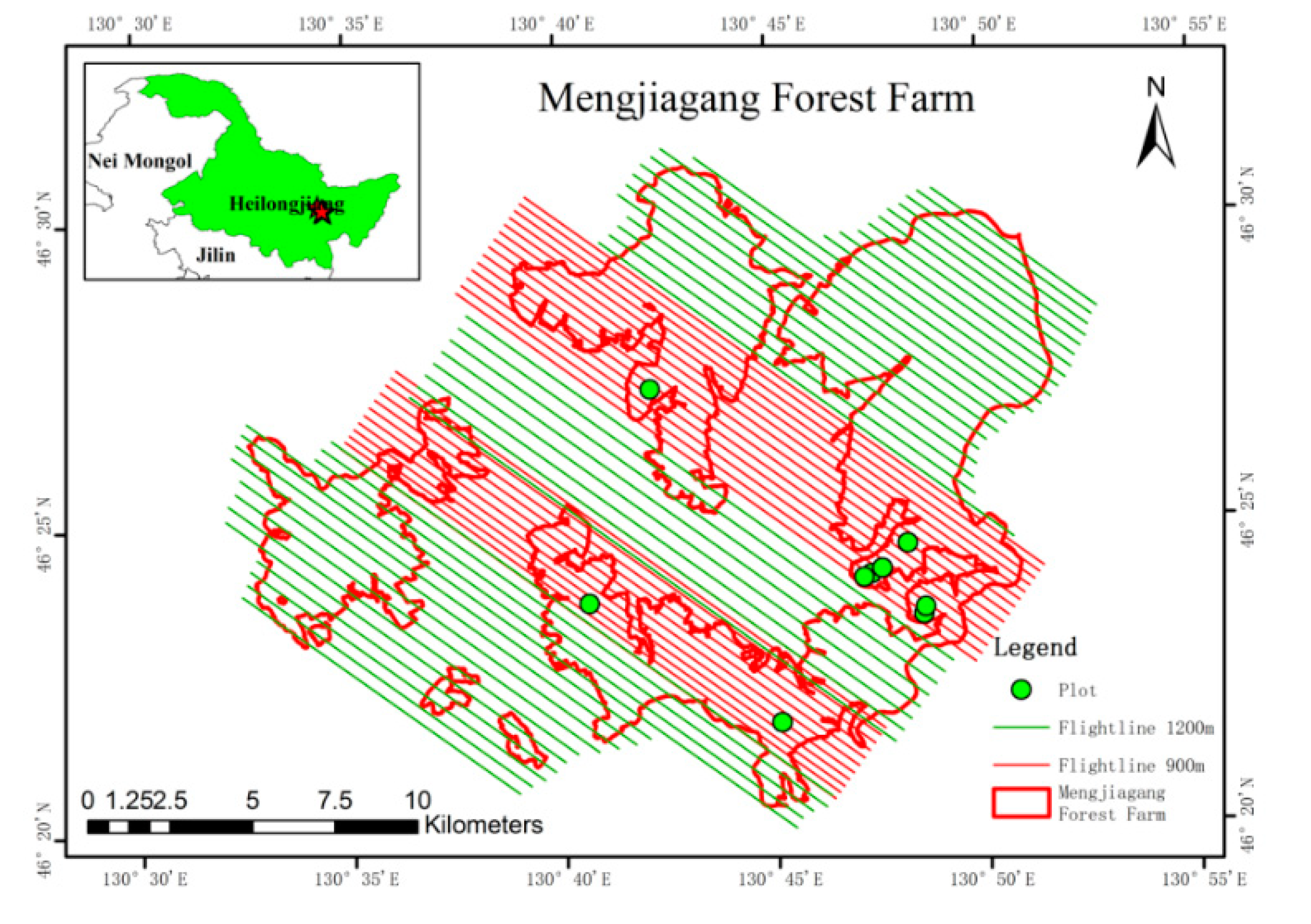
2.1. Study Area
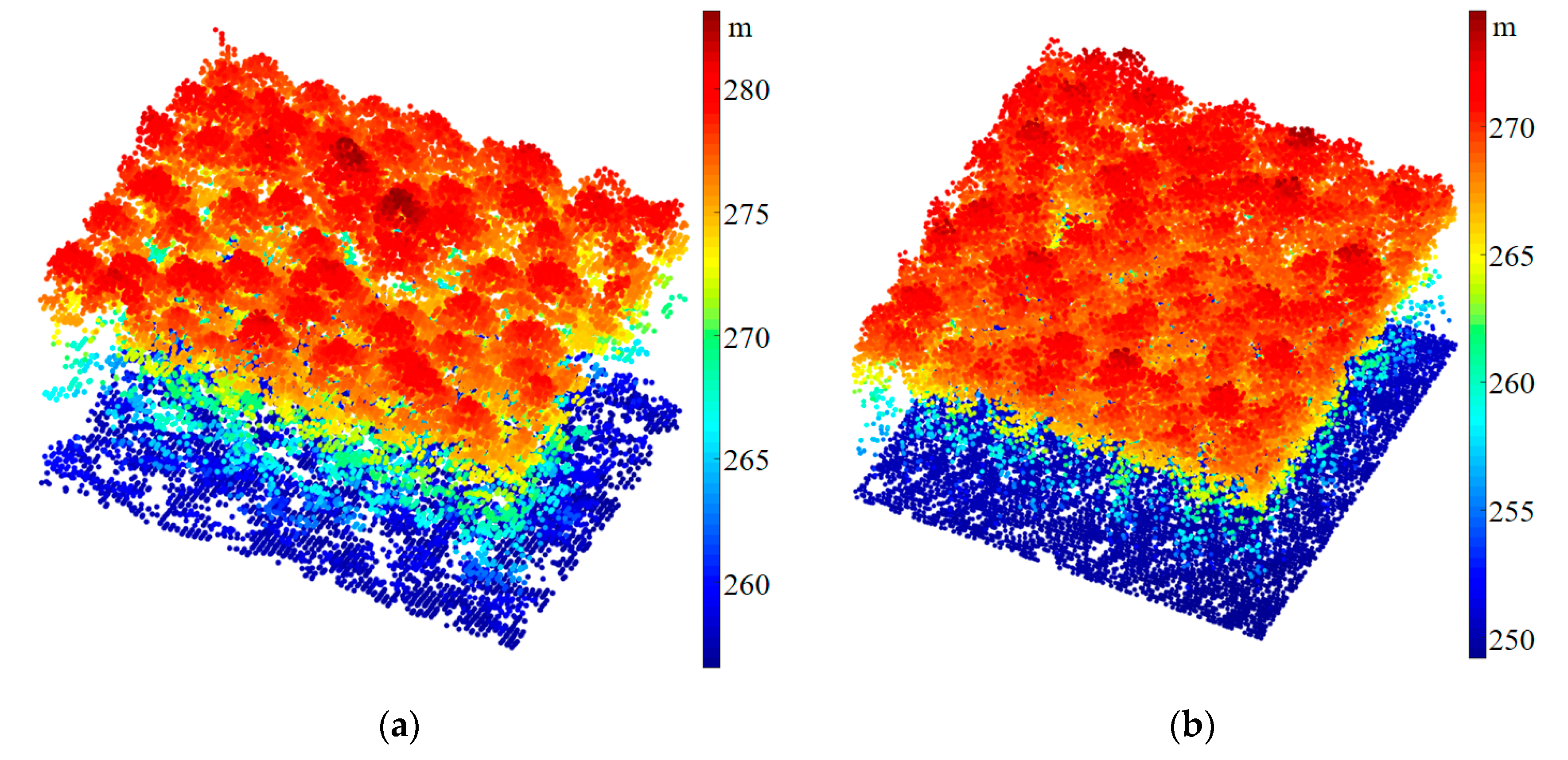
2.2. ALS Data
2.3. Ground Survey Data
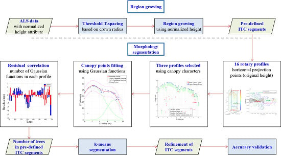
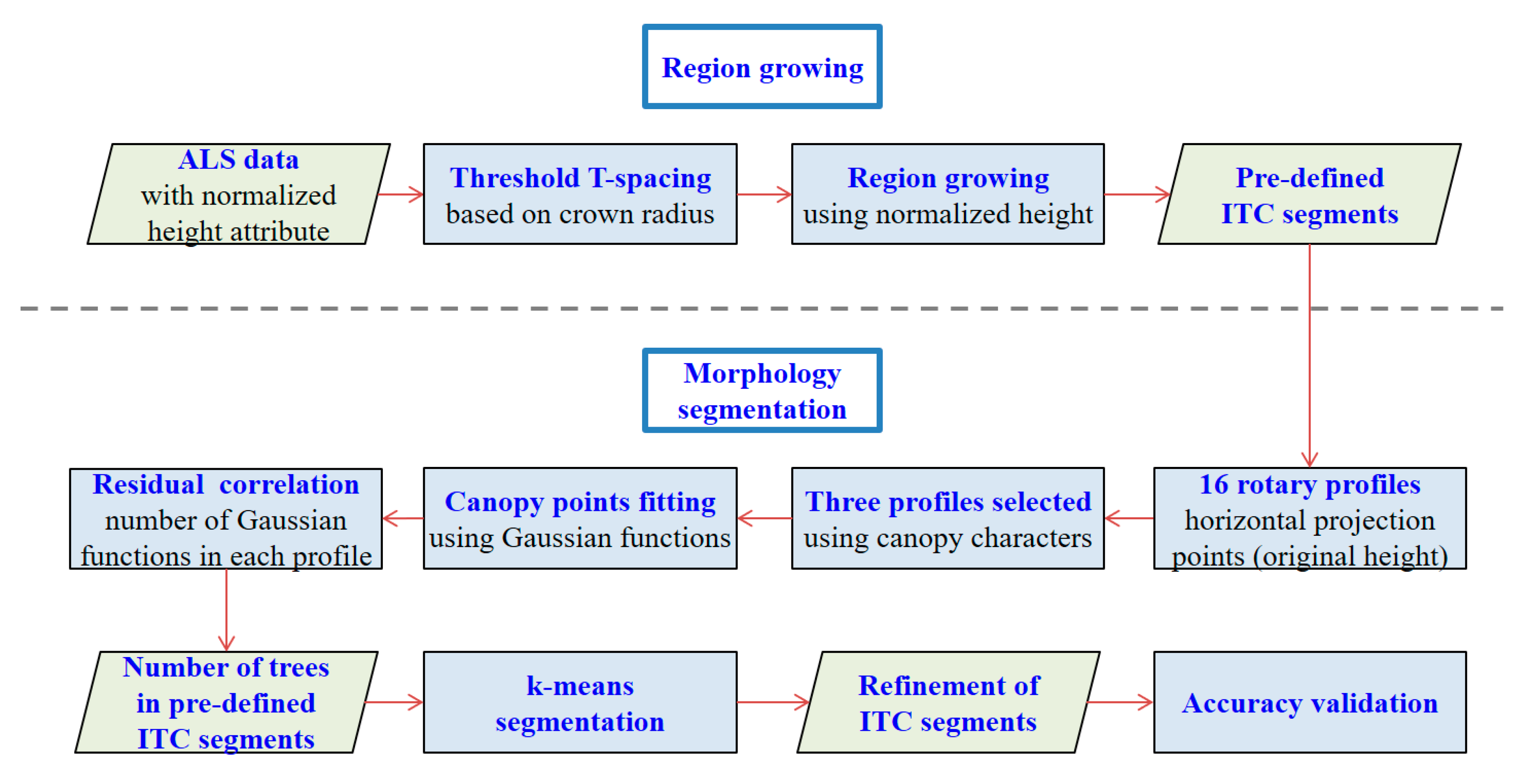
3. Methods
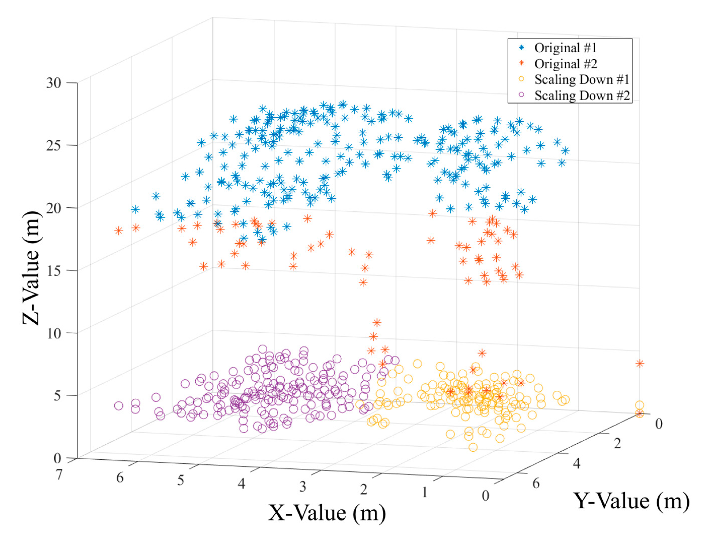
3.1. Region Growing
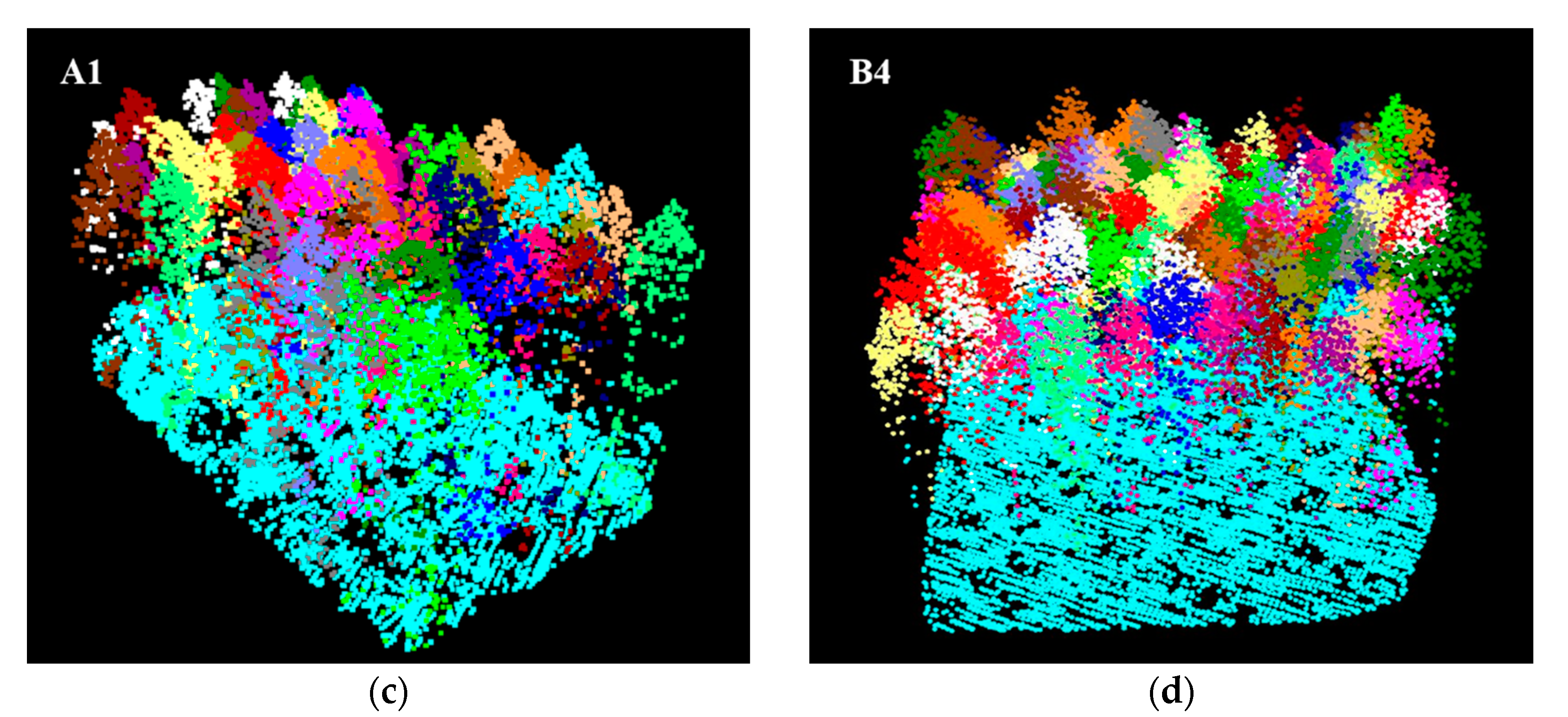
3.2. Segments Filter
3.3. Tree Number Definition Using the Profile Morphology
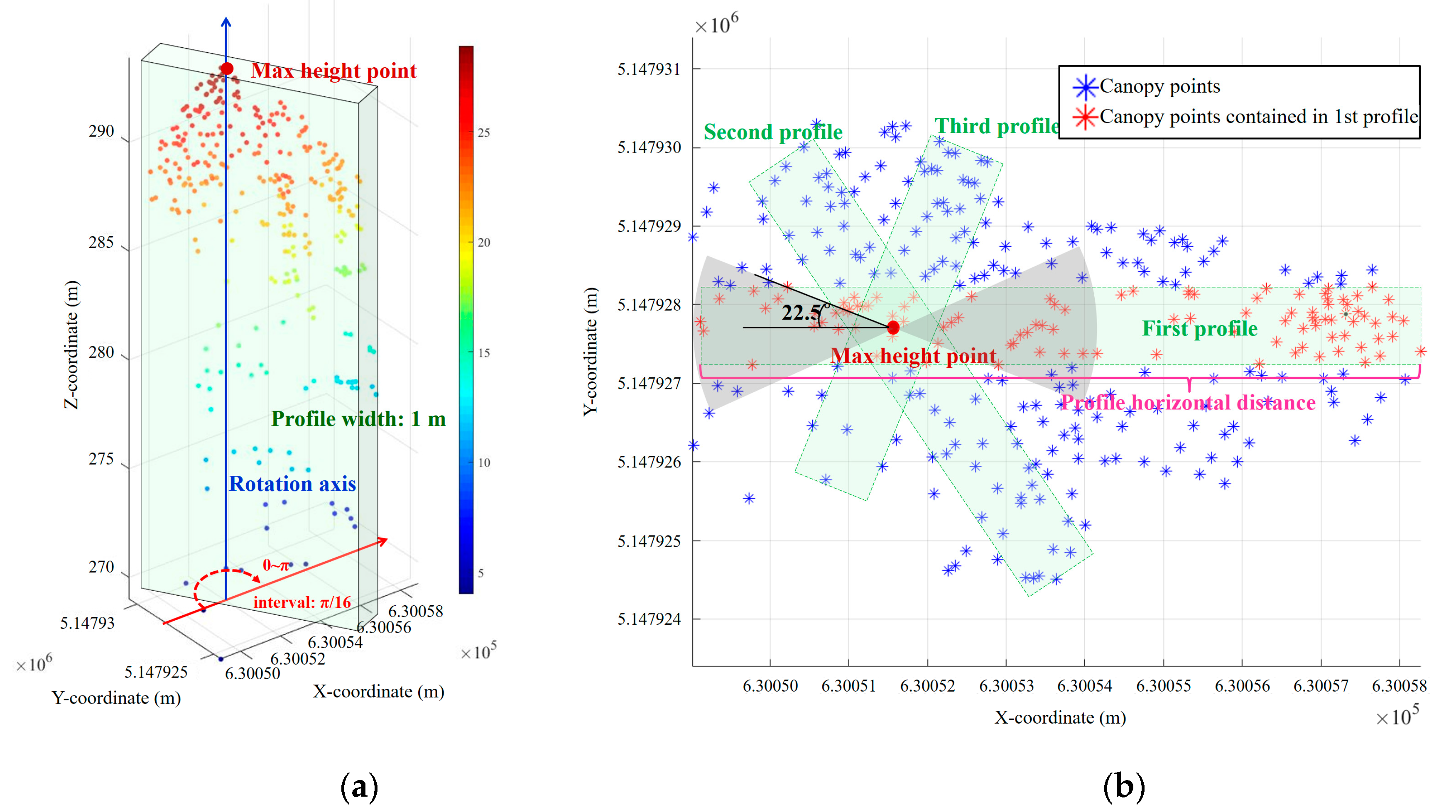
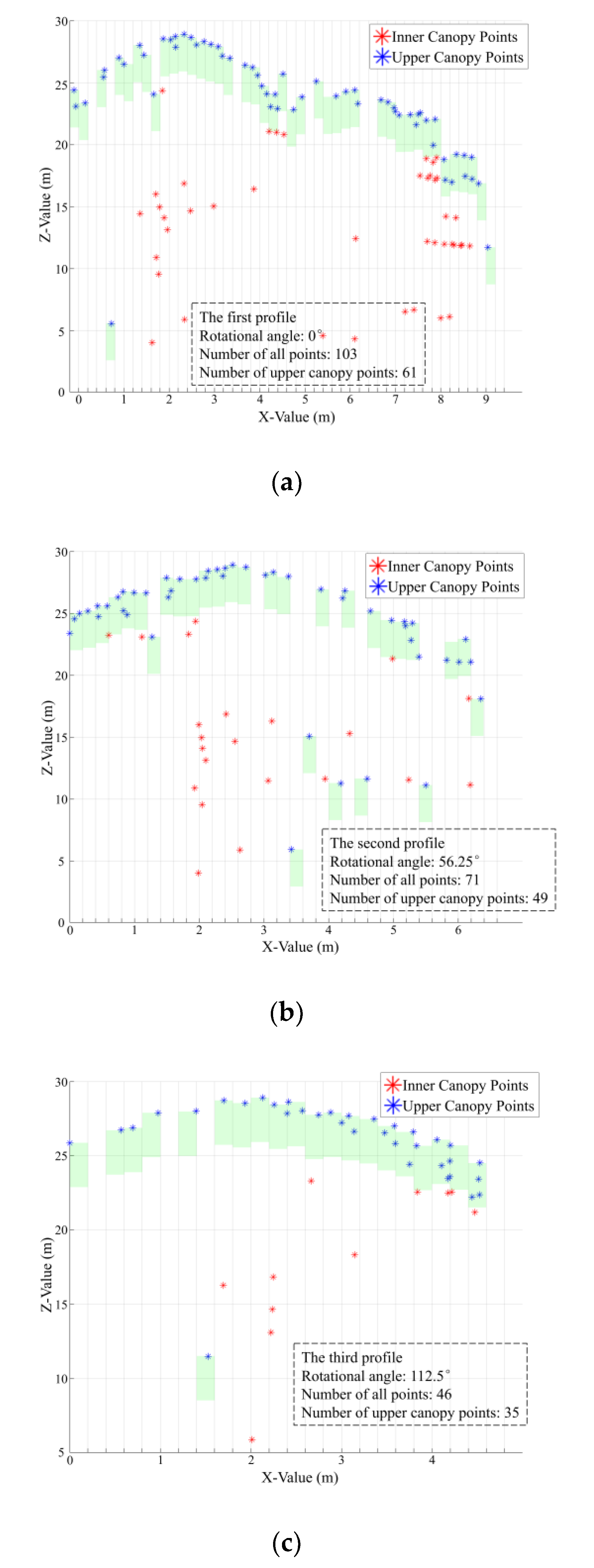
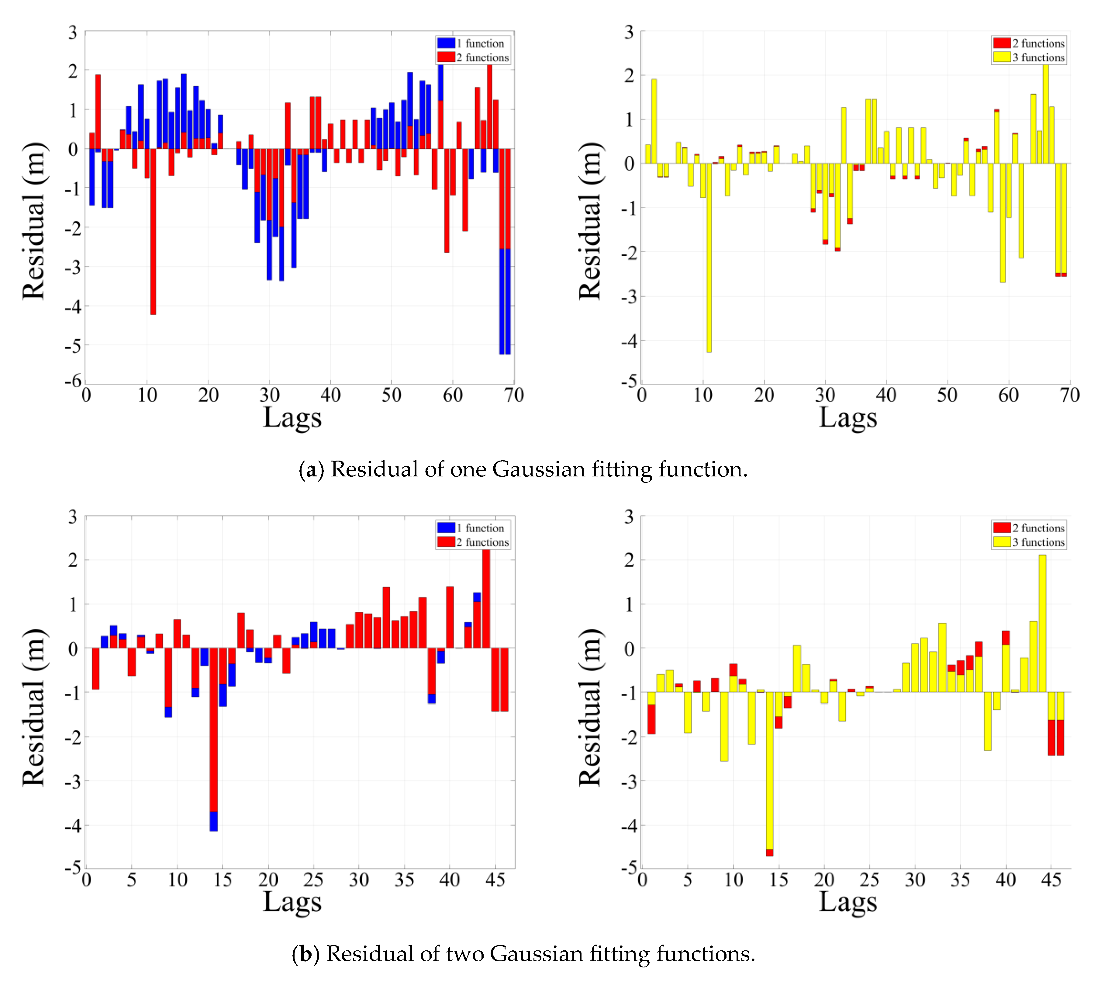
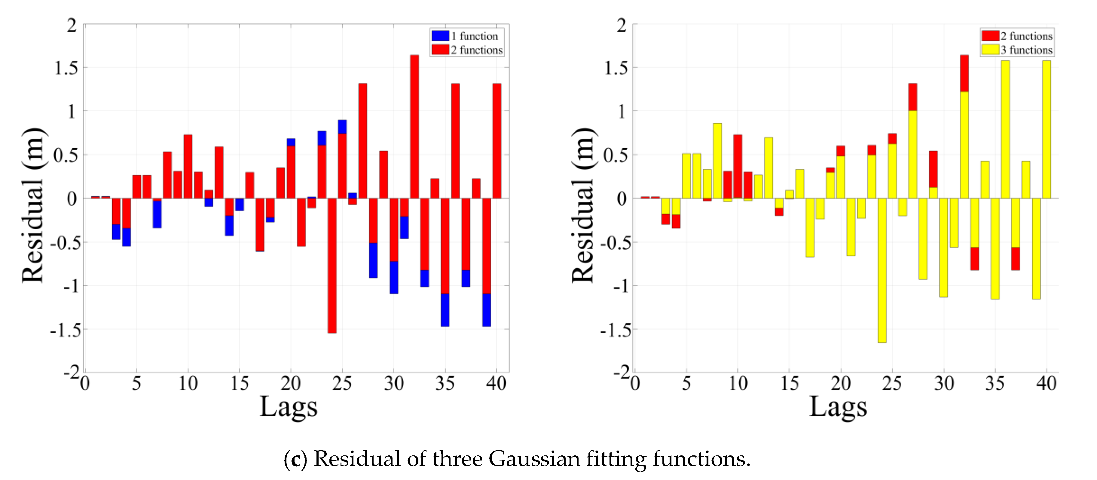
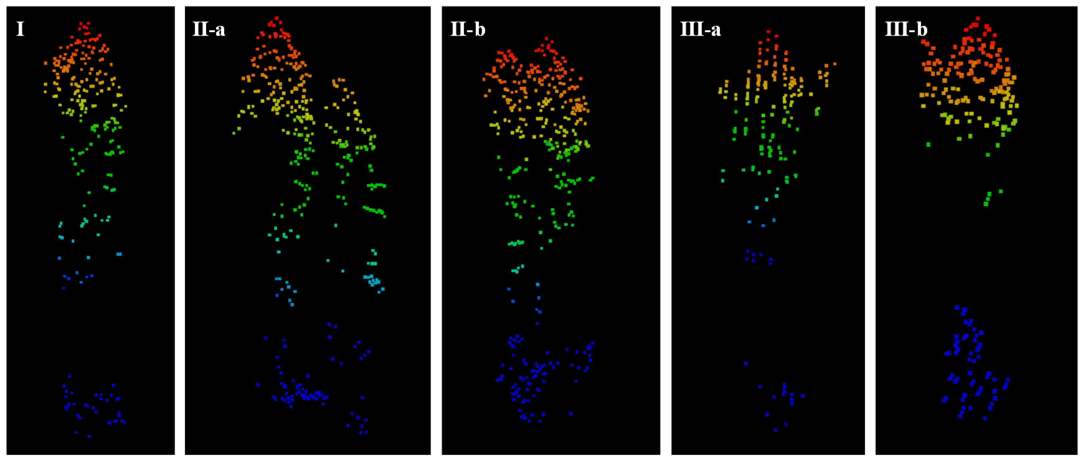
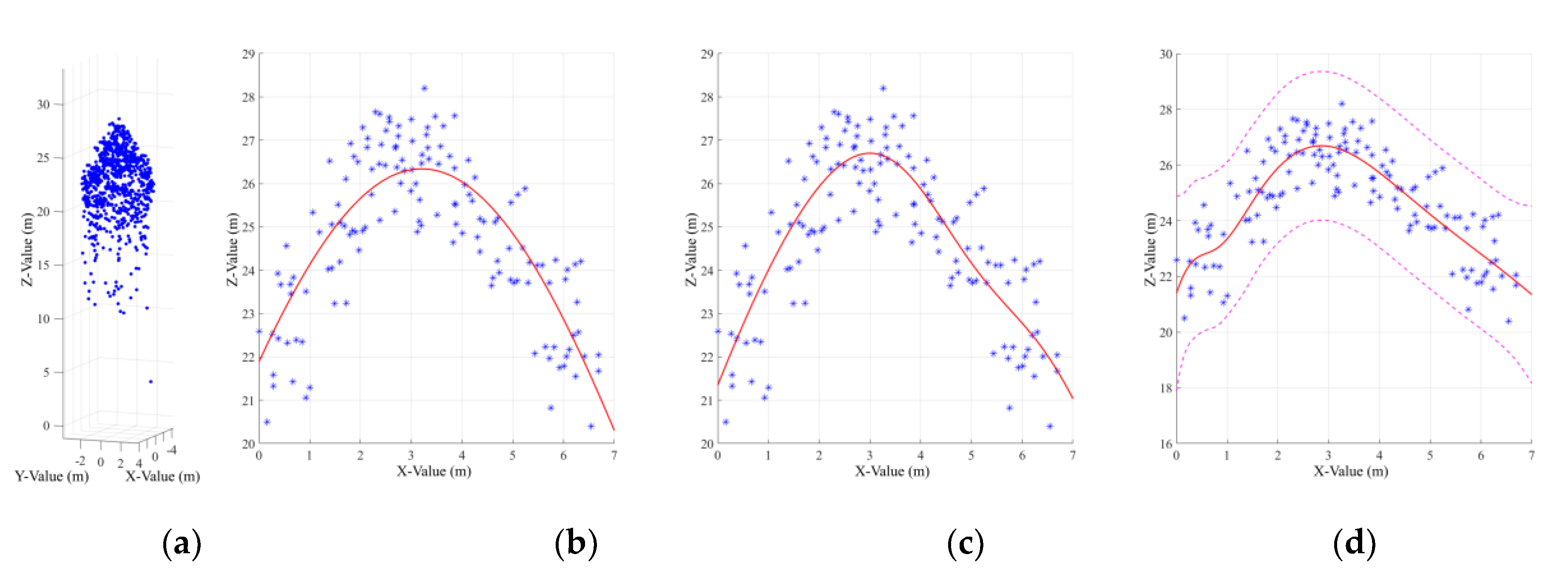
3.3.1. Profile Establishment
3.3.2. Profile Selection
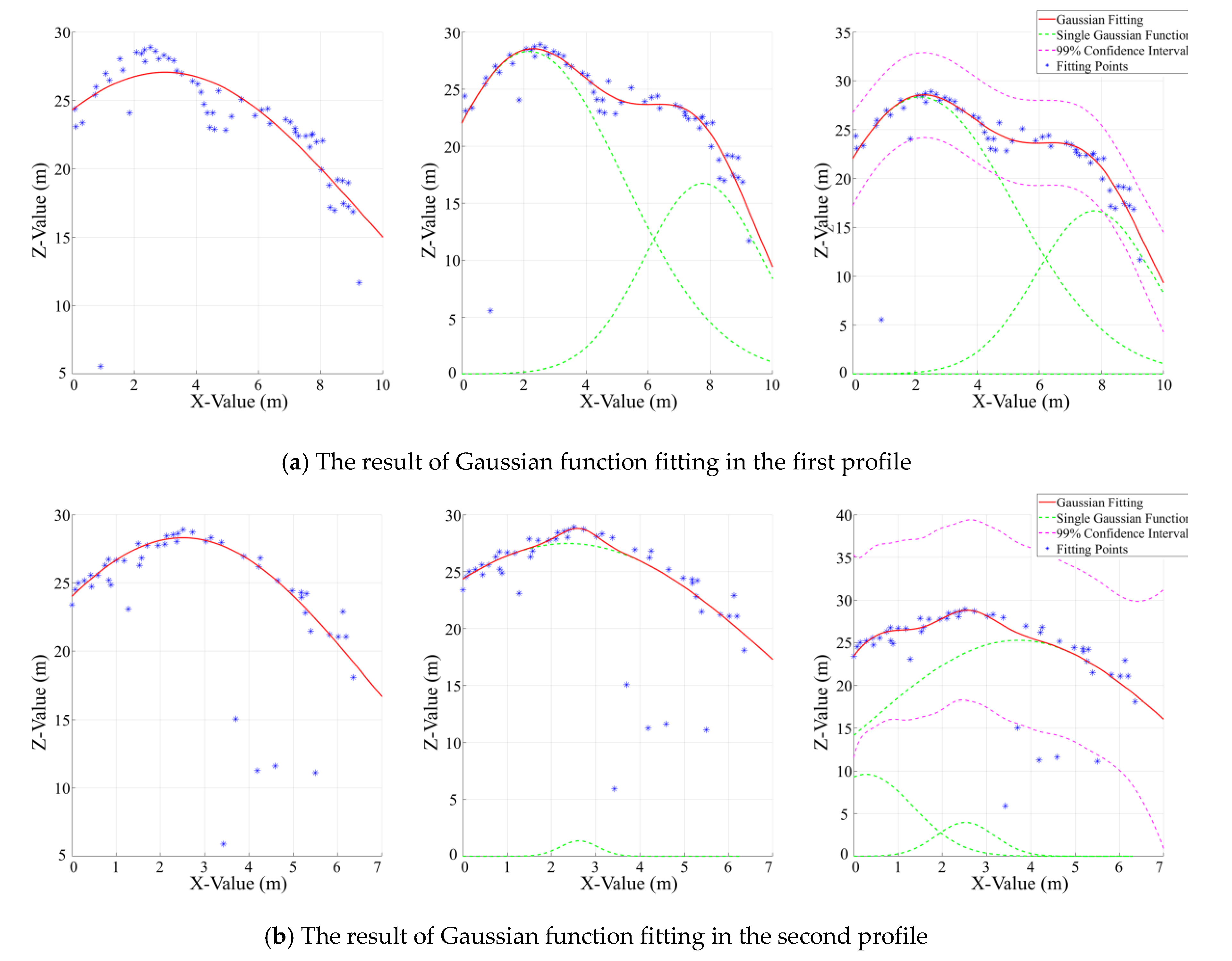
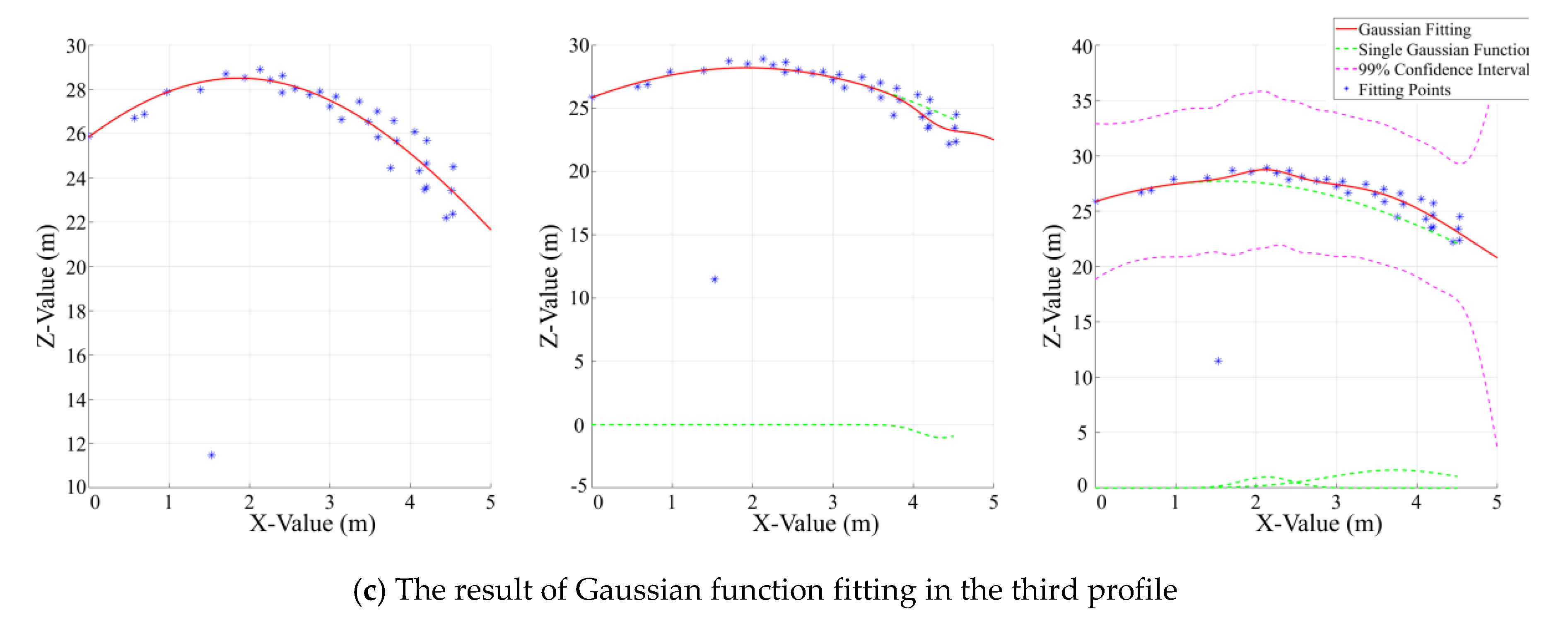
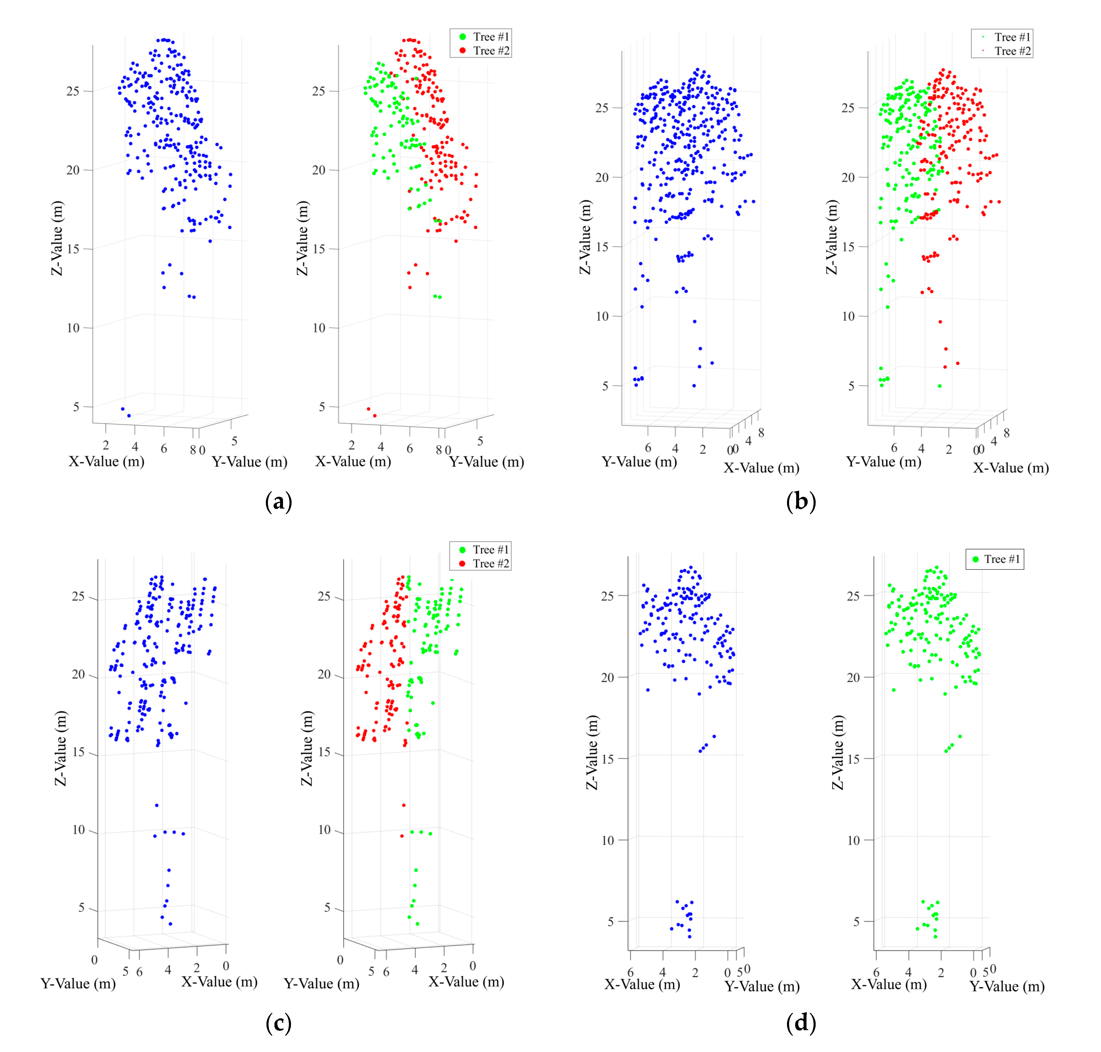
3.3.3. Tree Number Definition in Each Segment
3.4. k-Means Segmentation
3.5. Accuracy Evaluation
4. Results and Discussion
4.1. Accuracy of the ITC Segmentation
4.2. Discussion
4.2.1. Region Growing Segments
4.2.2. Morphology Segments
5. Conclusions
Author Contributions
Funding
Acknowledgments
Conflicts of Interest
References
- Sakurai, S. Plantation Forestry in the Tropics; Springer: Berlin, Germany, 1982. [Google Scholar]
- Walters, G.A. Saligna Growth in a 15-Year-Old Spacing Study in Hawaii; Research Paper PSW-RP-151; U.S. Department of Agriculture: Berkeley, CA, USA, 1980.
- Næsset, E.; Gobakken, T.; Solberg, S.; Gregoire, T.G.; Nelson, R.; Ståhl, G.; Weydahl, D. Model-assisted regional forest biomass estimation using LiDAR and InSAR as auxiliary data: A case study from a boreal forest area. Remote Sens. Environ. 2011, 115, 3599–3614. [Google Scholar]
- Rosenqvist, Å.; Milne, A.; Lucas, R.; Imhoff, M.; Dobson, C. A review of remote sensing technology in support of the Kyoto Protocol. Environ. Sci. Policy 2003, 6, 441–455. [Google Scholar] [CrossRef]
- Wulder, M.A.; White, J.C.; Nelson, R.F.; Næsset, E.; Ørka, H.O.; Coops, N.C.; Hilker, T.; Bater, C.W.; Gobakken, T. Lidar sampling for large-area forest characterization: A review. Remote Sens. Environ. 2012, 121, 196–209. [Google Scholar] [CrossRef] [Green Version]
- Wang, Y.; Hyyppä, J.; Liang, X.; Kaartinen, H.; Yu, X.; Lindberg, E.; Holmgren, J.; Qin, Y.; Mallet, C.; Ferraz, A.; et al. International benchmarking of the individual tree detection methods for modeling 3-D canopy structure for silviculture and forest ecology using airborne laser scanning. IEEE Trans. Geosci. Remote Sens. 2016, 54, 5011–5027. [Google Scholar] [CrossRef] [Green Version]
- Eysn, L.; Hollaus, M.; Lindberg, E.; Berger, F.; Monnet, J.-M.; Dalponte, M.; Kobal, M.; Pellegrini, M.; Lingua, E.; Mongus, D. A benchmark of lidar-based single tree detection methods using heterogeneous forest data from the alpine space. Forests 2015, 6, 1721–1747. [Google Scholar] [CrossRef] [Green Version]
- Unger, D.R.; Hung, I.-K.; Brooks, R.; Williams, H. Estimating number of trees, tree height and crown width using Lidar data. GISci. Remote Sens. 2014, 51, 227–238. [Google Scholar] [CrossRef]
- Harikumar, A.; Bovolo, F.; Bruzzone, L. An internal crown geometric model for conifer species classification with high-density lidar data. IEEE Trans. Geosci. Remote Sens. 2017, 55, 2924–2940. [Google Scholar] [CrossRef]
- Popescu, S.C.; Wynne, R.H.; Nelson, R.F. Measuring individual tree crown diameter with lidar and assessing its influence on estimating forest volume and biomass. Can. J. Remote Sens. 2003, 29, 564–577. [Google Scholar] [CrossRef]
- Richardson, J.J.; Moskal, L.M. Strengths and limitations of assessing forest density and spatial configuration with aerial LiDAR. Remote Sens. Environ. 2011, 115, 2640–2651. [Google Scholar] [CrossRef]
- Hyyppa, J.; Kelle, O.; Lehikoinen, M.; Inkinen, M. A segmentation-based method to retrieve stem volume estimates from 3-D tree height models produced by laser scanners. IEEE Trans. Geosci. Remote Sens. 2001, 39, 969–975. [Google Scholar] [CrossRef]
- Ene, L.T.; Næsset, E.; Gobakken, T.; Bollandsås, O.M.; Mauya, E.W.; Zahabu, E. Large-scale estimation of change in aboveground biomass in miombo woodlands using airborne laser scanning and national forest inventory data. Remote Sens. Environ. 2017, 188, 106–117. [Google Scholar] [CrossRef]
- Vauhkonen, J.; Næsset, E.; Gobakken, T. Deriving airborne laser scanning based computational canopy volume for forest biomass and allometry studies. ISPRS J. Photogramm. Remote Sens. 2014, 96, 57–66. [Google Scholar] [CrossRef]
- Erikson, M. Segmentation of individual tree crowns in colour aerial photographs using region growing supported by fuzzy rules. Can. J. For. Res. 2003, 33, 1557–1563. [Google Scholar] [CrossRef]
- Bongers, F. Methods to assess tropical rain forest canopy structure: An overview. In Tropical Forest Canopies: Ecology and Management; Springer: Dordrecht, The Netherlands, 2001; pp. 263–277. [Google Scholar]
- Popescu, S.C.; Wynne, R.H.; Nelson, R.F. Estimating plot-level tree heights with lidar: Local filtering with a canopy-height based variable window size. Comput. Electr. Agric. 2002, 37, 71–95. [Google Scholar] [CrossRef]
- Zhao, D.; Pang, Y.; Li, Z.; Liu, L. Isolating individual trees in a closed coniferous forest using small footprint lidar data. Int. J. Remote Sens. 2014, 35, 7199–7218. [Google Scholar] [CrossRef]
- Véga, C.; Durrieu, S.; Morel, J.; Allouis, T. A sequential iterative dual-filter for LiDAR terrain modeling optimized for complex forested environments. Comput. Geosci. 2012, 44, 31–41. [Google Scholar]
- Brandtberg, T.; Warner, T.A.; Landenberger, R.E.; McGraw, J.B. Detection and analysis of individual leaf-off tree crowns in small footprint, high sampling density lidar data from the eastern deciduous forest in North America. Remote Sens. Environ. 2003, 85, 290–303. [Google Scholar] [CrossRef]
- Korpela, I.; Tuomola, T.; Välimäki, E. Mapping forest plots: An efficient method combining photogrammetry and field triangulation. Silva Fenn. 2007, 41, 457–469. [Google Scholar] [CrossRef] [Green Version]
- Zhou, J.; Proisy, C.; Descombes, X.; Hedhli, I.; Barbier, N.; Zerubia, J.; Gastellu-Etchegorry, J.-P.; Couteron, P. Tree crown detection in high resolution optical and LiDAR images of tropical forest. In Proceedings of the Remote Sensing for Agriculture, Ecosystems, and Hydrology XII, Toulouse, France, 20–22 September 2010; p. 8240Q. [Google Scholar]
- Persson, A.; Holmgren, J.; Soderman, U. Detecting and measuring individual trees using an airborne laser scanner. Photogramm. Eng. Remote Sens. 2002, 68, 925–932. [Google Scholar]
- Solberg, S.; Næsset, E.; Bollandsas, O.M. Single tree segmentation using airborne laser scanner data in a structurally heterogeneous spruce forest. Photogramm. Eng. Remote Sens. 2006, 72, 1369–1378. [Google Scholar] [CrossRef]
- Pollock, R. The Automatic Recognition of Individual Trees in Aerial Images of Forests Based on a Synthetic Tree Crown Image Model. Ph.D. Thesis, University of British Columbia, Vancouver, BC, Canada, 1996. [Google Scholar]
- Popescu, S.C.; Zhao, K. A voxel-based lidar method for estimating crown base height for deciduous and pine trees. Remote Sens. Environ. 2008, 112, 767–781. [Google Scholar] [CrossRef]
- Falkowski, M.J.; Smith, A.M.; Hudak, A.T.; Gessler, P.E.; Vierling, L.A.; Crookston, N.L. Automated estimation of individual conifer tree height and crown diameter via two-dimensional spatial wavelet analysis of lidar data. Can. J. Remote Sens. 2006, 32, 153–161. [Google Scholar] [CrossRef] [Green Version]
- Koch, B.; Heyder, U.; Weinacker, H. Detection of individual tree crowns in airborne lidar data. Photogramm. Eng. Remote Sens. 2006, 72, 357–363. [Google Scholar] [CrossRef] [Green Version]
- Guo, Q.; Li, W.; Yu, H.; Alvarez, O. Effects of topographic variability and lidar sampling density on several DEM interpolation methods. Photogramm. Eng. Remote Sens. 2010, 76, 701–712. [Google Scholar] [CrossRef] [Green Version]
- Morsdorf, F.; Meier, E.; Allgöwer, B.; Nüesch, D. Clustering in airborne laser scanning raw data for segmentation of single trees. Int. Arch. Photogramm. Remote Sens. Spat. Inf. Sci. 2003, 34, W13. [Google Scholar]
- Sandeep, G.; Holger, W.; Barbara, K. Comparative analysis of clustering-based approaches for 3-D single tree detection using airborne fullwave lidar data. Remote Sens. 2010, 2, 968–989. [Google Scholar]
- Ferraz, A.; Bretar, F.; Jacquemoud, S.; Gonçalves, G.; Pereira, L.; Tomé, M.; Soares, P. 3-D mapping of a multi-layered Mediterranean forest using ALS data. Remote Sens. Environ. 2012, 121, 210–223. [Google Scholar] [CrossRef]
- Wang, Y.; Weinacker, H.; Koch, B. A lidar point cloud based procedure for vertical canopy structure analysis and 3D single tree modelling in forest. Sensors 2008, 8, 3938–3951. [Google Scholar] [CrossRef] [PubMed]
- Li, W.; Guo, Q.; Jakubowski, M.K.; Kelly, M. A new method for segmenting individual trees from the lidar point cloud. Photogramm. Eng. Remote Sens. 2012, 78, 75–84. [Google Scholar] [CrossRef] [Green Version]
- Polewski, P.; Yao, W.; Heurich, M.; Krzystek, P.; Stilla, U. Detection of fallen trees in ALS point clouds using a Normalized Cut approach trained by simulation. ISPRS J. Photogramm. Remote Sens. 2015, 105, 252–271. [Google Scholar] [CrossRef]
- Yao, W.; Krzystek, P.; Heurich, M. Tree species classification and estimation of stem volume and DBH based on single tree extraction by exploiting airborne full-waveform LiDAR data. Remote Sens. Environ. 2012, 123, 368–380. [Google Scholar] [CrossRef]
- Hu, B.; Li, J.; Jing, L.; Judah, A. Improving the efficiency and accuracy of individual tree crown delineation from high-density LiDAR data. Int. J. Appl. Earth Observ. Geoinf. 2014, 26, 145–155. [Google Scholar] [CrossRef]
- Dai, W.; Yang, B.; Dong, Z.; Shaker, A. A new method for 3D individual tree extraction using multispectral airborne LiDAR point clouds. ISPRS J. Photogramm. Remote Sens. 2018, 144, 400–411. [Google Scholar] [CrossRef]
- Pang, Y.; Li, Z.; Ju, H.; Lu, H.; Jia, W.; Si, L.; Guo, Y.; Liu, Q.; Li, S.; Liu, L.; et al. LiCHy: The CAF’s LiDAR, CCD and hyperspectral integrated airborne observation system. Remote Sens. 2016, 8, 398. [Google Scholar] [CrossRef] [Green Version]
- Wagner, W.; Ullrich, A.; Ducic, V.; Melzer, T.; Studnicka, N. Gaussian decomposition and calibration of a novel small-footprint full-waveform digitising airborne laser scanner. ISPRS J. Photogramm. Remote Sens. 2006, 60, 100–112. [Google Scholar] [CrossRef]
- Besl, P.J.; McKay, N.D. Method for registration of 3-D shapes. In Proceedings of Sensor Fusion IV. Control Paradig. Data Struct. 1992, 14, 586–607. [Google Scholar]
- Glira, P.; Pfeifer, N.; Briese, C.; Ressl, C. A Correspondence Framework for ALS Strip Adjustments based on Variants of the ICP Algorithm Korrespondenzen für die ALS-Streifenausgleichung auf Basis von ICP. Photogramm. Fernerkundung Geoinf. 2015, 4, 275–289. [Google Scholar] [CrossRef]
- Axelsson, P. Processing of laser scanner data—algorithms and applications. ISPRS J. Photogramm. Remote Sens. 1999, 54, 138–147. [Google Scholar] [CrossRef]
- Adams, R.; Bischof, L. Seeded region growing. IEEE Trans. Pattern Anal. Mach. Intell. 1994, 16, 641–647. [Google Scholar] [CrossRef] [Green Version]
- Sokolova, M.; Japkowicz, N.; Szpakowicz, S. Beyond accuracy, F-score and ROC: A family of discriminant measures for performance evaluation. Australas. Joint Conf. Artif. Intell. 2006, 4304, 1015–1021. [Google Scholar]
- Goutte, C.; Gaussier, E. A probabilistic interpretation of precision, recall and F-score, with implication for evaluation. Int. J. Radiat. Biol. Relat. Stud. Phys. Chem. Med. 2005, 51, 345–359. [Google Scholar]


| Plot ID | Mean DBH (cm) | Mean Height (m) | Min Height (m) | Max Height (m) | Crown Width East–West (m) | Crown Width North–South (m) | Stem Density (stems/ha) |
|---|---|---|---|---|---|---|---|
| A1 | 25.76 | 24.23 | 14.8 | 28.8 | 5.26 | 4.86 | 1216 |
| A2 | 31.48 | 28.93 | 23.1 | 33.1 | 5.01 | 5.00 | 1050 |
| A3 | 23.85 | 22.82 | 19.3 | 28.1 | 4.89 | 5.02 | 1367 |
| A4 | 21.67 | 22.19 | 17.3 | 26.2 | 4.21 | 3.36 | 1850 |
| B1 | 19.48 | 21.11 | 14.8 | 25.9 | 2.98 | 3.06 | 1617 |
| B2 | 17.65 | 20.58 | 15.1 | 26.4 | 2.65 | 2.78 | 1783 |
| B3 | 16.69 | 19.66 | 14.1 | 24.3 | 2.88 | 3.03 | 1817 |
| B4 | 15.56 | 19.92 | 13.1 | 27.2 | 2.77 | 2.80 | 2117 |
| Autocorrelation Coefficient | Profile 1 | Profile 2 | Profile 3 |
|---|---|---|---|
| Gaussian function 1–2 | 0.6433 | 0. 9396 | 0. 9687 |
| Gaussian function 2–3 | 0.9986 | 0.9505 | 0. 9362 |
| Plot Information | Region Growing Method | Morphology Segmentation Method | ||||||||||||||||
|---|---|---|---|---|---|---|---|---|---|---|---|---|---|---|---|---|---|---|
| Plot ID | Measured Tree | Density (num/ha) | Segment Trees | TP | FN | FP | c | r | p | F | Segment trees | TP | FN | FP | c | r | p | F |
| A1 | 63 | 1216 | 53 | 52 | 10 | 1 | 82.54% | 0.84 | 0.98 | 0.90 | 60 | 58 | 3 | 2 | 92.06% | 0.95 | 0.97 | 0.96 |
| A2 | 73 | 1050 | 68 | 67 | 5 | 1 | 91.78% | 0.93 | 0.99 | 0.96 | 72 | 70 | 3 | 2 | 95.89% | 0.96 | 0.97 | 0.97 |
| A3 | 82 | 1367 | 67 | 66 | 13 | 1 | 80.49% | 0.84 | 0.99 | 0.90 | 79 | 74 | 7 | 4 | 90.24% | 0.91 | 0.95 | 0.93 |
| A4 | 111 | 1850 | 78 | 75 | 30 | 2 | 67.57% | 0.71 | 0.97 | 0.82 | 97 | 93 | 8 | 4 | 83.78% | 0.92 | 0.96 | 0.94 |
| B1 | 97 | 1617 | 77 | 74 | 20 | 2 | 76.29% | 0.79 | 0.97 | 0.87 | 92 | 82 | 13 | 8 | 84.54% | 0.86 | 0.91 | 0.89 |
| B2 | 107 | 1783 | 86 | 79 | 22 | 3 | 73.83% | 0.78 | 0.96 | 0.86 | 96 | 89 | 12 | 6 | 83.18% | 0.88 | 0.94 | 0.91 |
| B3 | 109 | 1817 | 8 | 73 | 28 | 3 | 65.14% | 0.72 | 0.96 | 0.82 | 98 | 91 | 13 | 4 | 83.49% | 0.88 | 0.96 | 0.91 |
| B4 | 128 | 2117 | 82 | 80 | 32 | 1 | 62.50% | 0.71 | 0.99 | 0.83 | 114 | 106 | 19 | 6 | 82.81% | 0.85 | 0.95 | 0.89 |
| Total | 770 | / | 580 | 566 | 160 | 8 | 73.50% | 0.78 | 0.99 | 0.87 | 707 | 663 | 78 | 36 | 86.10% | 0.89 | 0.95 | 0.92 |
© 2020 by the authors. Licensee MDPI, Basel, Switzerland. This article is an open access article distributed under the terms and conditions of the Creative Commons Attribution (CC BY) license (http://creativecommons.org/licenses/by/4.0/).
Share and Cite
Ma, Z.; Pang, Y.; Wang, D.; Liang, X.; Chen, B.; Lu, H.; Weinacker, H.; Koch, B. Individual Tree Crown Segmentation of a Larch Plantation Using Airborne Laser Scanning Data Based on Region Growing and Canopy Morphology Features. Remote Sens. 2020, 12, 1078. https://0-doi-org.brum.beds.ac.uk/10.3390/rs12071078
Ma Z, Pang Y, Wang D, Liang X, Chen B, Lu H, Weinacker H, Koch B. Individual Tree Crown Segmentation of a Larch Plantation Using Airborne Laser Scanning Data Based on Region Growing and Canopy Morphology Features. Remote Sensing. 2020; 12(7):1078. https://0-doi-org.brum.beds.ac.uk/10.3390/rs12071078
Chicago/Turabian StyleMa, Zhenyu, Yong Pang, Di Wang, Xiaojun Liang, Bowei Chen, Hao Lu, Holger Weinacker, and Barbara Koch. 2020. "Individual Tree Crown Segmentation of a Larch Plantation Using Airborne Laser Scanning Data Based on Region Growing and Canopy Morphology Features" Remote Sensing 12, no. 7: 1078. https://0-doi-org.brum.beds.ac.uk/10.3390/rs12071078