Computer Vision and Deep Learning Techniques for the Analysis of Drone-Acquired Forest Images, a Transfer Learning Study

Abstract

Unmanned Aerial Vehicles (UAV) are becoming an essential tool for evaluating the status and the changes in forest ecosystems. This is especially important in Japan due to the sheer magnitude and complexity of the forest area, made up mostly of natural mixed broadleaf deciduous forests. Additionally, Deep Learning (DL) is becoming more popular for forestry applications because it allows for the inclusion of expert human knowledge into the automatic image processing pipeline. In this paper we study and quantify issues related to the use of DL with our own UAV-acquired images in forestry applications such as: the effect of Transfer Learning (TL) and the Deep Learning architecture chosen or whether a simple patch-based framework may produce results in different practical problems. We use two different Deep Learning architectures (ResNet50 and UNet), two in-house datasets (winter and coastal forest) and focus on two separate problem formalizations (Multi-Label Patch or MLP classification and semantic segmentation). Our results show that Transfer Learning is necessary to obtain satisfactory outcome in the problem of MLP classification of deciduous vs evergreen trees in the winter orthomosaic dataset (with a 9.78% improvement from no transfer learning to transfer learning from a a general-purpose dataset). We also observe a further 2.7% improvement when Transfer Learning is performed from a dataset that is closer to our type of images. Finally, we demonstrate the applicability of the patch-based framework with the ResNet50 architecture in a different and complex example: Detection of the invasive broadleaf deciduous black locust (Robinia pseudoacacia) in an evergreen coniferous black pine (Pinus thunbergii) coastal forest typical of Japan. In this case we detect images containing the invasive species with a 75% of True Positives (TP) and 9% False Positives (FP) while the detection of native trees was 95% TP and 10% FP.

1. Introduction

Forest ecosystems play an important role in water, carbon and nutrient cycling within the soil-vegetation-atmosphere continuum. In recent years climate change is exerting positive changes such as the early greening of forests in the northern hemisphere, shifting of forests to warmer environments northward [1] or negative ones, such as an increase of longer periods of drought [2], increase in the number of forest fires or extreme climate events [3]. Recent studies have focused on the ecological functions of mixed forests, since they show high resistance against insect outbreaks and a stronger capacity to recover from disturbances [4]. Detailed knowledge about mixed forest structure and composition [5] is needed in order to properly understand current status and future changes.

Forests in Japan occupy approximately 68% of the total territory, with most of them being natural deciduous broadleaf mixed forests [6]. Natural forests are affected by climate change while man-made forest ecosystems such as coastal forests are affected by invasive species that diminish their functions as windbreak [5,7]. The distribution of each species within a stand, or the interactions between the different tree species [4] makes them ecologically complex, especially in comparison to monoculture forests [8]. Until very recently, forest research has been carried out using labor and time-consuming land surveys [9]. They are costly and demand a high degree of organization training and expertise. Moreover, the characteristics of Japanese forests make them particularly challenging for land surveys as they are often located in steep mountain slopes that are difficult to access. Thus, new tools are needed in order to efficiently gain an overall understanding of species interaction and their response to climate change in order to design the proper response policy to ensure the sustainability of forests.

Unmanned Aerial Vehicles (UAVs) are rapidly becoming an essential tool in forestry applications [10,11,12,13] and they represent an easy-to-use, inexpensive tool for remote sensing of forests as they can fly close to tree canopies, which results in high image resolution (with one pixel representing a few centimeters). That can be processed by computer vision algorithms. An example of such an application is the building of orthomosaics by aligning the images for visualization and coherent processing of specific forest areas encompassing several hectares. From now on, and for the sake of brevity, we will refer to these orthomosaics simply as mosaics Additionally, emerging technologies such as Deep Learning (DL) allow the incorporation of expert knowledge to the automatic processing of images, which together with the availability of larger amount of data, has the potential to radically change the way land surveys are done. Namely, the time-consuming (and sometimes dangerous), intensive field surveys will likely become unnecessary, while those tasks requiring expert human knowledge are expected to be greatly increased.

1.1. State of the Art

Deep Learning is a part of Machine Learning that has gained much attention recently, resulting in a wide availability of data and software, making it the most easily accessible part of Artificial Intelligence. On the one hand, Deep Learning algorithms learn from examples: First, an architecture or set of nodes and connections among them is defined. The nodes in Artificial Neural Networks (ANN) are often grouped in layers and ANN with a large number of layers are called Deep Neural Networks (DNN). The type of each node, the number of nodes and the connections between them determine the behaviour of the network. Two main types of nodes exist: linear nodes, expressed as matrices and nodes that introduce non-linearity. The weights in linear nodes are typically initialised with random numbers. An important characteristic of ANN is that weights optimised for one problem can be used as the starting point to solve a new problem using less data. This is known as Transfer Learning [14]. After the network architecture has been defined and the weights have been initialised, the network is given example data. These data, known as training data contains instances of the problem being dealt with along with their solutions. The data are run through the network and the weights in all the linear nodes are changed following an optimization process.

Deep Learning was initially used to locate and classify different species of trees in mosaics built from UAV-acquired images in [10,11]. The authors used mosaics and Digital Elevation Models (DEM) to segment individual tree crowns [15], which were segmented and classified manually to build training data sets. These are two pioneering papers in the use of Deep Learning in forestry, however the insufficient amount of data appeared to hamper the sensitivity results reported in [10]. Since the number of images of individual trees used were about 900. This relatively small amount of data and the number of different tree species present in the forest resulted in a low number of images in each class, most notably in the test set (with some test classes having as few as 9 images). The data were also unbalanced, especially since the “other” class did not contain any trees. On the first set of results presented by the authors, there was low classification performance with 2 of the 6 tree classes not detected at all (0% reported sensitivity or recall, noted in the paper as “accuracy”) and the others ranging from 20% to 85% reported sensitivity, using data augmentation. This resulted in reported sensitivity values for tree classes ranging from 68% to 95%. However, this has a significant risk of over-fitting that was not addressed in the paper. The relatively large number of epochs used for training (30) also supported this possibility. These problems are also an issue in [11], although some steps were taken to mitigate them. The data used comprised three different data acquisition campaigns of the same area. In this case each class of test set contained the same number of trees (30). Results using only one mosaic presented low accuracy (50% on average for the three studied tree classes), [11] while presented results using all their acquired data and obtained results with average accuracy of 80%. Therefore, they demonstrated that more data could improve the classification results but also exemplified the difficulty of this issue. Safonova et al. [12] first predicted potential regions of trees in UAV images before classifying them into four degrees of parasite infestation. In this case, RGB images were chosen manually to build a balanced training data set that was expanded using data augmentation. Non-tree containing parts of the mosaic were filtered out using non-DL computer vision processing. Reported results showed remarkable high accuracy values from 76 to 92 % with an extensive use of different DL architectures. The paper of [12] provided an example of how careful data annotation and balancing could lead to highly accurate results in terms of detection. Fromm et al. [13] used DNN on their data to detect conifer seedlings. They evaluated trainings-set size, the influence of seasonality and seedlings size by considering spatial resolutions. In this case, the authors worked on single images instead of mosaics. Those were produced after manually labelling 200 seedlings in different phenological stages. Three DL-models were trained with the best performance provided by ResNet101. The models were improved by Transfer Learning and suitable results were obtained from a data set of only 500 images.

Our Contribution

The main goal of this paper is to study the use of Deep Learning to gain information on forestry applications. By dividing mosaics built using UAV-acquired images into regular patches and using two well-known DL architectures (ResNet and UNet), we propose the following objectives (see Figure 1 for an overview):

• Develop an algorithm (that uses a ResNet50) to classify patches corresponding to tree species (Multi-Label Patch (MLP) algorithm). Assess (a) Quality of the results obtained with the amount of data available (2800 images), and (b) Degree of improvement achieved by Transfer Learning.
• Develop a semantic segmentation algorithm for tree species that is precise (DICE coefficient) and efficient (computation time), using three separate algorithmic approaches and two DL networks.
• Evaluate the applicability of the MLP algorithm to another practical problem: Detection of an invasive tree species in a coastal forest.

To pursue these objectives we worked with two different in-house UAV-acquired datasets: Seven Winter mosaics of a mixed mountain forest and a mosaic of a pine tree plantation mixed with broad-leaf trees. We annotated the data and made it publicly available, at https://0-doi-org.brum.beds.ac.uk/10.5281/zenodo.3693326. The source code of our research is also available on demand. For our first objective, we used a MLP classification algorithm implemented using a ResNet50 architecture. We thoroughly studied the effects of learning rates (LR) on the output: (a) Not using Transfer Learning (b) Transfer Learning from ImageNet [16] and (c) Transfer Learning twice, first from ImageNet, then from the Planet satellite image dataset [17]. For the second objective we used three algorithms to obtain semantic (pixel-wise) segmentations of the deciduous vs. evergreen tree classes in winter mosaics: (1) The MLP algorithm as a standalone tool, (2) The MLP algorithm including a (non-DL) watershed segmentation refinement step and (3) A patch-based semantic segmentation algorithm using a UNet architecture.

The paper is organised as follows: Section 1.1 reviews the state of the art of DL applied to drone-acquired forestry images. Section 2 describes the data used in our study and provides details about the DL methodology used (problems solved, network architectures used). Section 3 contains experiments and a description of their results. In the first experiment, related to objective 1, we discuss the effects of Transfer Learning in tree species classification in winter mosaics. Then we discuss the effect of architecture and problem formalization by comparing our Resnet50 and UNet approaches (objective 2). Then we pursue objective 3 by using our MLP algorithm in a different application in the field of invasive tree species to show that the approach considered can be adapted to different practical problems. Section 4 provides interpretation of the importance of the results obtained and their implications for the research area. Finally, in Section 5 we summarize the main results and outline the main conclusions obtained in our study.

2. Methodology

Most of the forests considered for this study are natural (i.e., unmanaged) and located in steep mountainous areas that make field surveys difficult. In addition, forests deal with invasive tree species which have a major impact on the structures, properties and function of forest ecosystems [18]. The abundance of precipitation in the climate of Japan makes data gathering with drone missions challenging which limits the amount of data. Furthermore, we faced the problem of unevenly distributed trees making image recognition and segmentation tasks more complicated (previous studies of forests were performed mostly in plantations or well-managed forests located in flat areas see, for example [19]). Consequently, acquiring and annotating large datasets made up of millions of images such as ImageNet [16] was not feasible for us. Our research was, thus, motivated by the reported capacity of Deep Learning networks to work with smaller datasets as well as it has benefits from Transfer Learning.

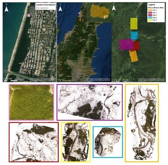
2.1. Data Acquisition

Having a sufficient amount of data is important for DL application. This study data were acquired using a drone (DJI Phantom 4), which is an easy-to-use, compact and lightweight drone equipped with a 12 megapixel stabilized camera that produces high-resolution geo-referenced images. The flights were performed with the autonomous mode, which standardized the acquisition protocol.

2.1.1. Location 1: Yamagata University Research Forest

Yamagata University Research Forest (YURF) is located on the main Island of Japan Honshu, covers an area of 750 ha and is crossed by the Wasada River (3833${}^{\prime }$21.4${}^{″}$N 13951${}^{\prime }$42.5${}^{″}$E). Sites close to the river are flat while the others are dominated by steep slopes reaching altitudes of 860 m. The forest is composed of mixed natural deciduous broad-leaf stands and man-made evergreen tree plantation [7]. The focus of this study is on mixed forest sites, which are located in lower altitude areas. For this location we decided to use the seasonality of mixed forests, by collecting images in the winter season aiming at gaining information on the locations of the stands of evergreen and deciduous trees. Additionally, the seasonal data provided information such as the number of deciduous tree stems (Section 2.2). Therefore, images were captured at three different dates in late winter 2018 presenting differences in illumination and tree age. We performed seven flights in five separate study sites (Figure 2). For site 1, three flights were done at different times in winter season, covering areas of 3 to 8 ha. The duration of the flights ranged between 15 and 33 min. A flight altitude of 80 m was chosen for flat areas while altitudes up to 205 m were used in the areas with steeper slopes. In order to improve the Ground Sampling Distance (GSD), which is the distance between centre points of each image of the ground expressed in cm/px, two flight plans where performed in steeper slope areas. GSDs between 2.79 and 4.48 (cm/pix) were achieved. The overlap of the images was adjusted for each flight and varying between 90 and 96 % of front and side overlap. The number of raw images was between 233 and 556 per site. We used the following abbreviations for our sites: mosaics wm3, wm4 and wm5 belong to the site 1 while the rest are all from different sites (wM1 = site 3; wM2 = site 2; wM6 = site 6; wM7 = site 4).

2.1.2. Location 2: Shonai Coastal Forest

The second study site was located in the coastal area of Shonai Region (Figure 2) (3852${}^{\prime }$35.6${}^{″}$N 13947${}^{\prime }$54.3${}^{″}$E). This is a 150-year-old black pine (Pinus thunbergii) coastal forest plantation [7]. Black pines are evergreen trees with a high tolerance to acidity, alkalinity and salty soils, as well as drought conditions [7,20]. This forest was planted to protect the surrounding area from strong winds and sand movements. From the early 1990s this forest has been invaded by black locust trees (Robinia pseudoacacia) that is expected to weaken their windbreak potential. This tree species is well-known for its rapid growth and the high biomass production with a high impact on the structure and function of tree communities because of its leguminous features [7]. The task with this forest is to precisely detect the location of invasive tree species in order to analyse their distribution and impact on the coastal forest. Therefore, we performed one flight in summer 2019 collecting, approximately, 1000 images at a flight altitude of 30 m covering an area of 2.8 ha.

2.2. Data Processing and Annotation

The raw images acquired by the drone were processed using Metashape software [21]. This software uses multi-view 3D reconstruction algorithms to align the pictures taken by the drone creating image mosaics and producing DEMs. We generated seven mosaics of the forest site in YURF and one mosaic for the coastal forest. The annotation process was done manually using GIMP [22] image manipulation software in the form of binary layers belonging to each class. The classes were decided by objects/characteristics that we were able to identify on the images. We used this annotation method, that needed 4 to 7 hours per mosaic as a simple, relatively fast way of annotating data for general applications. For the mixed forest winter mosaics five layers were annotated: River, Man-made, Uncovered, Deciduous and Evergreen (Figure 3). For the coastal mosaics four layers were annotated: “Black locust”, “Soil”, “Other trees” (containing black pine trees) and “Man-made” (Figure 4). The ”other trees” classes corresponded mainly to pine trees but included also a small number of trees from other species. The manual annotations were used as ground truth data.

We then divided each of our mosaics into axis-aligned, square patches of the same side length (hereafter size of the patch) (Figure 3). We considered the annotations as well as the original data, obtaining a set of patches along with patch-wise binary masks for each annotated class.

Any algorithm used in a practical setting is heavily influenced by the characteristics of the data. In our case, the disposition of the forest (see Section 2.1) prevented us from using Ground Control Points (GCP). GCPs are meant to be geo-localised easily distinguishable points that aid mosaicking software identify corresponding regions in different images during mosaic construction. Sites presenting dense and unmanaged forests (Figure 5B,F) prevent the placement of GCPs inside the forest making the use of GCPs impractical. Also derived from tree distribution, Figure 5B shows the difficulties to identify single trees. However, the use of winter mosaics (Figure 5A) shows an image of the same area where stems are visible and their numbers can be counted. Furthermore, the orography of the forest made data acquisition limited in terms of the amount of data that could be gathered. Figure 5C is an example of one of the steep slopes that are common in this area. This picture also shows deciduous trees in different conditions and frequently mixed with other classes. The understory vegetation present has the same colour of the deciduous tree and often appears mixed with them. A similar problem happens with the “River” class in Figure 5A. Another limitation likely resulting from not using GCPs is that Metashape produced some image registration artefacts (Figure 5C,D,G). This increased the difficulty of automatically processing the images. Images F to H present examples in the coastal forest. Image G shows black locust trees while image H shows examples of black pine and other trees of the area. The trees in this mosaic present only small differences in colour and structure. Image H shows that black locust trees are often smaller than black pine trees and therefore often covered by them.

2.3. Problem Formalization

The automatic division of the data and mosaic-level annotations into regular patches allowed us to formalize our problems in two different ways. First, we focused on identifying what classes where present in each mosaic patch, which is known as multi-label classification (Section 2.4). As a second formalization we focused on classifying each pixel in each mosaic patch. This problem is known as semantic segmentation [23]. The aforementioned patch multi-label classification algorithm already gave us an initial “coarse” approximation to this semantic segmentation. In order to refine it we used the classical watershed [24] image segmentation method (Section 2.4.1). We also considered the UNet DL architecture [25] (Section 2.5). A full pipeline of our work is provided in Figure 6, while Figure 7(left) shows a patch of one of the winter mosaics. The central part of the Figure 7 shows the manual annotation for this patch. Blue pixels are classified as the “Evergreen” class, yellow pixels to the “Uncovered” class and green pixels as the “River” class.

2.4. Multi-Label Patch Classification Using ResNet

Previous studies have shown the efficiency of DL networks to classify forestry images, specifically, [10,11] because they rely on the ResNet architecture [26]. We used the ResNet variant with 50 layers, known as ResNet50. Although the aforementioned approaches used a tree crown segmentation step that used the DEM produced by the drone, we decided to work only with RGB data to emphasize our focus on image data. We considered our data and annotations divided into patches and each patch was assigned a list containing the classes in it. For example, the list in the case of the patch visible in Figure 7 would be river, uncovered and evergreen. Thus, patches may belong to more than one class each with a probability value for each patch. Given high enough probabilities in more than one class, the patch would be "labelled" repeatedly. Thus, this algorithm will be referred to as the MLP based classifier. The ResNet50 network was then trained to classify these patches. A subset of the data was used for training and the remaining data was used to validate the quality of the trained model at predicting the correct classes. Eighty percent of the dataset was randomly chosen for training and the remaining 20% was used for testing (Section 3).

DL architectures need less data than previous approaches, however, having sufficient data to produce results of satisfactory quality is still a problem in research areas such as forestry, where data acquisition is often problematic. Transfer Learning represents a way to improve the quality by initializing the weights of the matrices conforming the DL network to those obtained in the solution of a similar problem. In our study we used Transfer Learning from: (1) a general-purpose object classification problem codified in the ImageNet database [16] and (2) the closer problem of multi-label classification in satellite images of the amazon forests codified in the Planet dataset [17] (see Section 3.1).

2.4.1. Segmentation Refinement Using watersheds

The multi-label patch classification algorithm described generated an initial “coarse” segmentation. All pixels in any patch containing a class would be considered to belong to that class. This patch-wise masks for all classes constitute a segmentation of the mosaic. The “coarse” nature of this segmentation produces two problems. On the one hand, over-segmentation: by assigning all the pixels in the patch to all the classes present, would surely assign pixels to classes they did not belong to. These extra pixels make the masks of classes larger. On the other hand, the coarse class masks therefore generated intersect. This is undesirable in the semantic segmentation problem as each pixel should be classified into one single class. In order to improve the initial segmentation we implemented a refinement step based on the watershed image segmentation algorithm [24]. This algorithm uses binary images representing initial masks consisting of doubtless labelled pixels. Parts of the image that we could confidently assigned to the background were also determined. Any pixel not falling into any of these two cases were labelled as “unknown”. Labelled regions were visualised as ridges and unknown areas as basins. Then, water was pictured as expanding from the ridges into the basins until two of the growing ridges meet and watershed lines were determined. These lines defined the segmentation.

In our case, we worked at mosaic level starting with the coarse segmentation of the “River” class. A binary image was generated from it by painting all pixels black that belonged to all patches where the river class had been predicted. All pixels out of these patches were marked as background. Then, this coarse mask was shrunk using a distance transform and pixels that had been deleted by this process were labelled as unknown. Further, all the connected components of the mask were computed and stored in a dictionary with their position and an identifier, along with the information that they belonged to the “River” class. Then, we considered the second class, the “Deciduous” class. The previous process was repeated but storing the results from the previous step. Regions that previously formed the background were overwritten, regions that were unknown before or where two labels were assigned were labelled as unknown. The process was repeated for all classes and the images were partitioned into (1) Background (2) unknown and (3) initial regions. Each initial region had the information attached as to what class it belonged to. The watershed algorithm was subsequently run to create a finer segmentation without intersection between the different classes.

2.5. Forest Mosaic Segmentation Using UNet

The UNet Deep Learning architecture [25] was originally developed for medical image segmentation ([27]) but has since then been used in a variety of applications. The UNet architecture is composed of two parts known as “paths”: the encoder and the decoder path. The encoder path extracts features using convolutional layers and reduces the size of the images using max pooling layers. At the end of the encoder path the images are greatly reduced in size and the transformations they were subjected to are stored in the weights of the matrices along the path. The decoder path, moves back to full size ones by replacing pooling operators with upsampling operators. High resolution features from the encoder path were combined with the upscaled output in order to localize them. Successive convolution layers learn to re-assemble the output more precisely based on this information. An algorithm was implemented using the UNet architecture to perform semantic segmentation of the winter mosaics. We considered the data and pixel-wise-annotation patches described in Section 3 and used them to train a UNet network. Whenever a new mosaic needed processing, (1) we divided it in patches, (2) predicted the semantic segmentation of each patch using the trained UNet model and (3) joined all patch segmentations together to obtain a semantic segmentation for the whole mosaic.

2.6. Evaluation Criteria

We used several metrics to evaluate different aspects of our algorithms performance. First, the capacity of the MLP algorithm to correctly predict the labels in every patch was evaluated: Full Agreement (FA): Stands for the percentage of patches where the predicted labels matched exactly those in the ground truth. Full Agreement with False Positives (FAFP): In this case all ground truth classes were correctly predicted but some intrusive classes were added. Partial Agreements (PA): Patches where some but not all of the correct classes were predicted and where some classes might have been added. Finally, the complementary of this measure (when the sets of ground truth and predicted labels had no intersection) was considered No Agreement (NA).

In order to target the predictive capacities of our algorithms we considered patch labels for the MLP algorithm and pixel labels for the semantic segmentation algorithm. For all of them we considered the relation between predicted values and real values as stated in the ground truth and broke them into the usual classifications of True Positives: TP, False Positives: FP, True Negatives: TN, False Negatives: FN. Furthermore, and in order to focus on the classes of most practical interest (evergreen and deciduous for winter mosaics and black locust and other trees for the coastal forest mosaic) classification measures were computed on them: Sensitivity, Specificity and Accuracy. In order to evaluate semantic segmentation results, the DICE coefficient that considers the ground truth mask and the predicted mask to define TP, FP, TN and FN pixels was used. Subsequently, it compares the number of correctly predicted positives (TP) with the number of errors (FP + FN).

$$\begin{array}{c}SENS=\frac{\mathrm{TP}}{\mathrm{TP}+\mathrm{FN}}SPEC=\frac{\mathrm{TN}}{\mathrm{TN}+\mathrm{FP}}ACC=\frac{\mathrm{TP}+\mathrm{TN}}{\mathrm{TP}+\mathrm{TN}+\mathrm{FP}+\mathrm{FN}}DICE=\frac{2TP}{2TP+FP+FN}\end{array}$$

3. Results

In this section, we present experiments using real data corresponding to seven winter mosaics and one summer mosaic from the coastal forest covering a total area of 38.5 ha. Of the five winter mosaics from YURF, three corresponded to the same site on different days and under different lighting conditions. All the algorithms described throughout the paper were implemented using the python programming language. The ResNet and UNet DL architectures were implemented using the Fastai [28] library. The watershed algorithm was implemented using the opencv computer vision library [29]. All experiments where run in workstation using a Linux Ubuntu operating system with 10 dual-core 3GHz processors and an NVIDIA GTX 1080 graphics board. For experiments 1 and 3 the data were randomly divided into (80%, 20%) training and validation/testing. For experiment 2 a leave-one-out approach was done with each of the seven winter mosaics using one for validation/testing and the other six for training.

3.1. Experiment 1: Transfer Learning and Multi-Label Patch Classification

The data were randomly divided into (80%, 20%) training and validation/testing. The patch size was chosen to be 150, see Section 3.2 for the effect of this parameter. With this parameter, the annotated patches contained the deciduous label in 52.26% of the cases, the evergreen class in 39.33%, uncovered in 28.29%, river in 12.84% and man-made in 1.26%. Notice that, as patches often belong to more than one class, these percentages add to more than 100%.

In order to assess the impact of Transfer Learning several "starting models" were built and trained using our images. Each model was considered in two forms, frozen and unfrozen. When a frozen model was re-trained only the final layers of the model were changed. When an unfrozen model was re-trained, all of the layers were modified. The starting models that we considered were:

• Random: In order to test whether Transfer Learning was necessary, we included a model initialised with random weights. Only results of the unfrozen random model were presented as the frozen random model had poor results.
• RN50F, RN50UNF: We also considered a ResNet50 with preloaded ImageNet [16] weights. The inclusion of this model allowed us to study whether or not a general-purpose classification model could be fit to solve our problem using a relatively low number of images. This model was re-trained frozen (RN50F) and unfrozen (RN50UNF).
• RN50 + PLANET-UNFF, RN50 + PLANET-UNFUNF, RN50 + PLANET-FF, RN50 + PLANET-FUNF: We also considered the ResNet model again and re-trained it using the PLANET dataset of satellite images of the Amazon rainforest [17]. In order to assess whether better results could be obtained when training from a problem (classification of satellite images of tropical vegetation) being more similar to our data. The ResNet model was considered frozen and unfrozen as before, RN50 + PLANET-F, RN50 + PLANET-UNF. These two models were subsequently retrained with our images each considered frozen and unfrozen producing 4 models: RN50 + PLANET-UNFF, RN50 + PLANET-UNFUNF, RN50 + PLANET-FF, RN50 + PLANET-FUNF.

The learning rate of a DL model is a parameter that controls the step size of the optimizer that changes the weights in each iteration of the training phase. We tested various LR values in all the different Transfer Learning approaches. In order to present a comprehensive picture, among all values tested we present (Figure 8) those from $1\times {10}^{-5}$ to $0.9$ with 10 sampling points at each exponent value ($1\times {10}^{-5},2\times {10}^{-5}...9\times {10}^{-5},1\times {10}^{-4},2\times {10}^{-4}...$).

Agreement: Agreement results (TA, TAFP, PA) provided us with a general picture of the capacity to all the trained models to classify our patches with all the possible labels (River, Deciduous, Uncovered, Evergreen and Man-made). The best TA results were obtained by the RN50+PLANET-UNFUNF model with a value of 81.58 at a learning rate of $4\times {10}^{-3}$. The first trend that could be observed in plots A,B,C in Figure 8 is that the learning rate that provides better result for a model is determined by whether the model was frozen or not. Specifically, the three unfrozen models obtained best results with smaller learning rates of around $1\times {10}^{-4}$ while frozen models achieve their best results with learning rates of 0.04. This is consistent with previous results reported in [10] where the best learning rate for a frozen model trained using ImageNet weights was 0.01.

The importance of Transfer Learning was indicated in the TA peaks of the different approaches. The model initialised with random weights peaked at 72.53 TA, a lower value than the other models. Frozen models achieved good results with models RN50F, RN50+PLANET-FF and RN50+PLANET-UNFF peaking at 79.51, 79.42 and 79.62 TA, respectively. This represented an improvement of 9.78% over the model with random weights. Similar trends could be observed for the accumulated TAFP and PA plots with peaks of 87.76 TAFP and 98.12 PA for the RN50+PLANET-UNFF model. Likewise, similar results could be observed with unfrozen models. Best results of RN50UNF, RN50+PLANET-FUNF and RN50+PLANET-UNFUNF peaked at 80.39, 80.98 and 81.58 TA. This was an improvement of 10.83%, 11.66% and 12.48% over the random weights model. Best overall results were obtained from the model that was built using first an unfrozen version of the ImageNet model to train the Planet dataset and then leaving the resulting model unfrozen to train with our images. The general tendencies observed here were confirmed using difference of means hypothesis tests (t-tests as data size was > 25). Even models presenting smaller differences in the TA peak (like the difference between the performance of the RN50UNF and RN50+PLANET-UNFF) were found to present statistically significantly different means with significance level 0.05.

Classification of deciduous and evergreen classes: The best TA was obtained with the RN50+PLANET-UNFUNF and a value of 81.58%. Patches without Total Agreement presented errors when classifying the three classes that were not of direct practical interest (river, uncovered, man-made). The number of patches containing them was low compared to patches presenting the other two classes (deciduous and evergreen. However, the results of our two classes of interest had high sensitivity, specificity and accuracy values (plots D, E, F in Figure 8, average values for the two classes) so we did not perform data balancing. Best average accuracy results between the two classes (94.80%) were obtained by the RN50+PLANET-UNFUNF model (that also obtained the top TA value). The clearly defined boundaries of evergreen trees resulted in an accuracy of 97.24%, while the deciduous tree class presented less defined edges and obtained 92.36%. Sensitivity and specificity values of the same model were also high with an average of 94.38% (94.75% Ev, 94.01% Dec) and 94.50% (98.73% Ev, 90.27% Dec). The larger difference appeared in specificity, where we observed an 8% difference. This can be explained by misclassifications of the deciduous class into mainly the uncovered class. Still, the classification results were high with values of up to 97%. This indicated that our patch-dividing and classification approach using a multi-label ResNet DL classifier was successful with our amount of data.

3.2. Experiment 2: Semantic Segmentation

We present results from three approaches, the patch based coarse segmentation produced by the algorithm in Section 2.4, the refinement of that segmentation using watershed segmentation and the patch-based UNet algorithm presented in Section 2.5. The first goal of this experiment was to test the performance of the algorithms in real-life conditions. We trained our models with data from six mosaics and validated (tested) with the one that had been left out. This approach relates to the use case where an already trained system receives a new mosaic for automatic classification. Of our seven mosaics three belonged to the same site. Consequently, in most cases (4/7), test images were of trees that the trained system had never seen before. In some other (3/7) images of trees previously seen under different conditions where used for testing. These two sets of results allowed us to discuss about the generalization power of our algorithm and the possibility of over-fitting. As a second major goal, we studied what the effect of choosing one problem formalization or DL architecture over another had in the insights gained from the data.

Patch size and learning rate: The proximity of the multi-label patch classifier (seen as a coarse segmentation) output to the manual annotations depended on two factors: First, the accuracy of the classification model, where wrongly classified patches would result either in False Positive or False Negative regions in our coarse mask and second the size of the patches, which produced an approximation error that grew with the size of the patches. At the same time, smaller patches took longer to compute. We considered patch sizes from 500 to 25 for both ResNet Patch based classification (known as “coarse” segmentation) and the version with Watershed refinement (noted “Refined”). The learning rate presented was the highest among all learning rates studied in Section 3.1 for each patch size. The training time needed for the Resnet varied from under 10 minutes for patch size 500 to two hours fifty minutes for patch size 100 up to over 40 hours for patch size 25. Concerning the UNet, we tried several patch sizes and learning rates where the patch size of 500 led to better results. In this study we only present five illustrative examples of learning rates.

Table 1. Comparison of semantic segmentation approaches for the “Deciduous” class in winter mosaics (wM*). The first half of the table contains the results for the UNet model, the second half contains results from the patch based multi-label ResNet classifier. The first column contains the size of the patches used. Rows marked "Coarse" use only the ResNet classifier while rows marked “Refined” also use watershed refinement. Last two columns are the average values (AVG) between all mosaics and between mosaics of site 1.

Deciduous		wM1	wM2	wM3	wM4	B	wM6	wM7	AVG	AVG Site1
UNet
LR 0.3		0.253	0.222	0.000	0.402	0.254	0.329	0.397	0.265	0.219
LR 0.04		0.607	0.171	0.372	0.537	0.494	0.275	0.308	0.395	0.468
LR 0.003		0.650	0.631	0.571	0.448	0.429	0.254	0.326	0.473	0.483
LR 0.0005		0.824	0.772	0.797	0.609	0.596	0.664	0.699	0.709	0.667
LR $6\times {10}^{-5}$		0.792	0.740	0.784	0.591	0.637	0.639	0.620	0.686	0.671
Resnet
Patches 500	Coarse	0.665	0.572	0.659	0.569	0.666	0.492	0.521	0.592	0.631
	Refined	0.704	0.597	0.695	0.501	0.583	0.510	0.568	0.594	0.593
Patches 300	Coarse	0.581	0.515	0.604	0.555	0.594	0.441	0.398	0.527	0.584
	Refined	0.585	0.505	0.501	0.552	0.666	0.450	0.449	0.530	0.573
Patches 200	Coarse	0.684	0.576	0.687	0.609	0.670	0.559	0.514	0.614	0.656
	Refined	0.720	0.613	0.708	0.510	0.597	0.555	0.616	0.617	0.605
Patches 100	Coarse	0.795	0.702	0.777	0.683	0.767	0.702	0.698	0.732	0.742
	Refined	0.796	0.703	0.780	0.681	0.764	0.707	0.704	0.733	0.741
Patches 50	Coarse	0.860	0.779	0.782	0.711	0.790	0.761	0.753	0.777	0.761
	Refined	0.667	0.614	0.514	0.570	0.670	0.432	0.509	0.568	0.585
Patches 25	Coarse	0.896	0.839	0.752	0.711	0.795	0.78	0.757	0.790	0.753
	Refined	0.706	0.6	0.448	0.562	0.611	0.494	0.488	0.558	0.540

and

Table 2. Comparison of semantic segmentation approaches for the “Evergreen” class in winter mosaics (wM*). The first half of the table contains the results for the UNet model, the second half contains results from the patch based multi-label ResNet classifier. The first column contains the size of the patches used. Rows marked “Coarse” use only the ResNet classifier while rows marked "Refined" also use watershed refinement. Last two columns are the average values (AVG) between all mosaics and between mosaics of site 1.

Evergreen		wM1	wM2	wM3	wM4	wM5	wM6	wM7	AVG	AVG Site1
UNet
LR 0.3		0.856	0.822	0.364	0.576	0.708	0.785	0.620	0.676	0.549
LR 0.04		0.894	0.806	0.798	0.767	0.828	0.769	0.612	0.782	0.797
LR 0.003		0.855	0.802	0.803	0.626	0.761	0.763	0.648	0.751	0.730
LR 0.0005		0.931	0.896	0.906	0.815	0.897	0.928	0.876	0.893	0.873
LR $6\times {10}^{-5}$		0.914	0.857	0.859	0.794	0.866	0.896	0.818	0.858	0.840
Resnet
Patches 500	Coarse	0.607	0.650	0.511	0.528	0.593	0.644	0.644	0.597	0.544
	Refined	0.676	0.710	0.548	0.375	0.604	0.700	0.729	0.620	0.510
Patches 300	Coarse	0.697	0.729	0.651	0.634	0.661	0.723	0.691	0.684	0.648
	Refined	0.804	0.345	0.744	0.708	0.676	0.800	0.809	0.698	0.709
Patches 200	Coarse	0.722	0.767	0.638	0.619	0.697	0.736	0.710	0.698	0.651
	Refined	0.845	0.850	0.759	0.722	0.769	0.807	0.721	0.782	0.750
Patches 100	Coarse	0.865	0.844	0.796	0.767	0.806	0.847	0.803	0.818	0.789
	Refined	0.887	0.869	0.884	0.689	0.873	0.907	0.877	0.855	0.815
Patches 50	Coarse	0.914	0.888	0.867	0.820	0.865	0.904	0.852	0.873	0.851
	Refined	0.844	0.744	0.880	0.514	0.523	0.865	0.735	0.729	0.639
Patches 25	Coarse	0.923	0.875	0.881	0.84	0.89	0.926	0.843	0.883	0.870
	Refined	0.424	0.529	0.621	0.514	0.55	0.656	0.675	0.567	0.562

present the DICE coefficient for all the algorithm variants. The average training time of the UNet was of over 11 hours.

DICE coefficient: Concerning semantic segmentation for all sites, the best results for the UNet were (0.709,0.893) DICE for (deciduous,evergreen) for LR=0.0005. The ResNet50 coarse segmentation obtained (0.790,0.883) for patch size 25 with the refined version (watershed post-processing) reaching (0.733,0.855). On the other hand the UNet semantic segmentation achieved and average value of 0.893 for the "Deciduous" class, showing how its pixel wise approach adapts better to this class that presents less well defined borders. The learning rates presented for the UNet show some representative examples of all the learning rates considered.

The Refined ResNet algorithms, watershed post-processing helped to improve the coarse segmentation up to a certain patch size. For these models, the training time was the fastest among the three models and the results obtained were not far from the best obtained. This represents an example of specialized computer vision algorithms that can complement the knowledge gained by using DL. These algorithms, however, cannot easily be used by non-experts and require careful fine-tuning as exemplified by the failure of the watershed refinement to produce satisfactory results for small patch size. This was most likely due to small misclassified regions growing into larger regions due to poor parameter choice than actual limitations of the proposed approach. However, running the watershed refinement took less than a minute for any of the tested mosaics. Training time of the UNet network or any of the networks with smaller patch sizes was much larger than that.

The difference of the average DICE coefficient among sites were small. Mosaics 3, 4 and 5, representing site 1, show differences of 6% for the with UNet network defined “Deciduous” class. An improvement of 1% for the same mosaics and classes with the refined ResNet algorithm was attained.

3.3. Experiment 3: Detection of Invasive Tree Species in the Coastal Forest

We tested whether the general approach regarding data handling, annotation and problem formalization considered in this paper could be used to solve other practical problems. The winter mosaic application is an example of a classification problem of trees with no leaves (deciduous) against trees with full leaf cover (evergreen). This is an interesting problem that has multiple applications as for instance the classification of trees attacked by insects outbreaks in relation to healthy trees [12]. We collected data related to a problem of class differentiation in a dense green forest. In this section the MLP algorithm was trained for pine trees, with green-yellowish leaves from black locust, presenting a light green broadleaf. The shape of the leaves was visible on the mosaic but not easy to tell apart even by experts (Figure 9). As the main interest in practice is to detect the occurrences of black locust, we grouped pine trees and a small number of trees from other tree species into a class called “other trees”. This is a complex problem in image classification terms as the differences between these “other trees” and the black locust were minor. Moreover, the distribution of the invasive species within the forest was irregular and often made up of very small patches sometimes including single trees. Furthermore, the coastal forest dataset showed a ratio of 90:10 between the “other trees” and “black locust” class.

As in experiment 2, we ran the experiment only with the ResNet50 with the ImageNet weights considered frozen and unfrozen. The models were retrained using the coastal forest data and the results with the highest accuracy were obtained with the unfrozen model. Figure 10 presents representative examples of the results obtained.

A 75% rate of True Positives for black locust and less than 10% False Positives (90.826 True Negative rate) was achieved (Figure 10 right side). At the same time, the other trees were detected with over 95% True Positive rate and about 10% of False Positives. These results provided valuable insight into the problem of detecting black locust trees in mixed forests. Furthermore, the remainder of the results indicated that, by using DL tools in a more sophisticated approach or complementing it with computer vision algorithms, these insights could likely be improved. For example, learning rate $2\times {10}^{-3}$, obtained a high TA (90.8) with only 62% sensitivity for the "black locust" class. This version of the classifier presents low False Positive recognizing values for both classes and, thus, high accuracy by largely ignoring the black locust class, which is less frequent. This was already apparent in Figure 9 but we computed that the “other trees” class appeared 10 times more frequently than the “black locust” class. The TA value in this case (42.78) was low but the sensitivity value of the “black locust” class was the highest in the whole experiment reaching almost 85%. This resulted in a high confusion between the “black locust” and “other trees” classes, with the specificity of the "black locust" class dropping to about 65%.

4. Discussion

In our first experiment, the effects of Deep Learning were quantified concerning the problem of multi-label patch classification of winter mosaics. The available seven mosaics were an insufficient amount of data to reach high accuracies for tree species classification when training a ResNet network from scratch. Precisely, starting from random weights led to a TA value of 72.53. Our experiments showed that Transfer Learning from ImageNet (a general-purpose dataset) was essential to obtain high quality results with a 9.78% improvement in Total Agreement (up to 79.63 TA). Ref. [13] reported a similar increase in conifer seedling detection metrics ranging between 3% and 10%. Additionally, a further 2.7% improvement in our Total Agreement (reaching 81.58 TA) was observed when Transfer Learning from the Planet dataset, which is more closely related to our images (Section 3.1, Figure 8). Thus, Transfer Learning is necessary to obtain reliable results for our winter mosaics problem. Furthermore, the smaller improvement when Transfer Learning from the Planet dataset was performed (2.7% over 9.78%) suggests that dedicating too many resources to find closely related problems may not be cost-effective. Furthermore, these results indicated that making data and annotations from forestry-related Deep Learning research publicly available could speed up the development of this research area by decreasing the amount of data needed by future contributions.

In the last step of experiment 1 we focused on the results of only evergreen and deciduous trees since tree species classification was the aim of our study. High accuracy, sensitivity and specificity values were achieved. Specifically, regarding sensitivity, evergreen trees reached values of 94.75% and deciduous trees reached 94.01%. Comparing these results to previous work is difficult as previous studies have used single-label (rather than) multi-label classification. Also, they have used different DL networks, applied in problems with different levels of complexity [10,11,12]. Nevertheless, and for the sake of context, we present our obtained sensitivity values with these previous works in

Table 3. Comparison with State of the Art methods.

Onishi and Ise 2018		Safonova et al. 2019		Natesan et al. 2019		Our Results
Classes	Sens.%	Classes	Sens.%	Classes	Sens.%	Classes	Sens.%
Deciduous broadleaf	95.83	Healthy	100.00	Red Pine	67.00	Deciduous	94.75
Deciduous coniferous	84.62	Colonized	86.11	White Pine	77.00	Evergreen	94.01
Evergreen broadleaf	68.00	Recently died	81.25	None Pine	97.00
Chamaecyparis obtusa	91.95	Deadwood	100.00
Pinus elliottii/taeda	94.12
Pinus strobus	88.89
Others	88.20
Average	89.00		91.84		81.00		94.38

. Specifically, [10,11] reached average sensitivities of 89% and 81%, which were lower than the ones achieved in our experiment. Ref. [12] reached an average value of 91.84%, which was close to our results but the single classes showed a high variability from 81.25% to 100%.

Our second experiment focused on segmentation approaches of the “Deciduous” and “Evergreen” classes. Best DICE values for these two classes with UNet were (0.709,0.893) and with ResNet (0.790,0.883). These numbers showed that the best results were obtained by UNet for the “Evergreen” class while the "Deciduous" class was better detected by the MLP ResNet approach. The less-defined borders and the overlap between colours of the deciduous trees and the “Uncovered” class makes it difficult to properly segment the trees with the pixel-oriented UNet. In this sense, formalising the problem as a patch labelling problem allowed us to gain some flexibility in the definition of the classes and identify the pixels belonging to this class more precisely. On the other hand, formalising the problem as a semantic segmentation problem allowed us to use the internal coherence of the “Evergreen” class. In addition, the comparison between the DICE coefficients of all mosaics suggests that our algorithms were able to segment totally new mosaics as well as those that they had already seen under other lighting conditions. Overfitting, then, seems not to be present in our results and we could confirm that our algorithms can segment deciduous and evergreen trees in Japanese mixed forest with reasonably good results. Furthermore, the watershed-based refining step provided a fast compromise between the two pure-DL formalizations. Consequently, using larger patch size with watershed refinement might be a solution in situations where training time is a limiting factor. This problem-specific computer vision algorithm illustrates the effect that a more sophisticated use of DL and computer vision techniques can have on forestry research.

In our last experiment we assessed the performance of our simple patch-based approach for solving practical problems such as tree class differentiation. We obtained a 75% rate of True Positives for the “black locust” class with under 10% of False Positives while simultaneously obtaining (95%, 10%) values for the “other trees” class. This showed that DL can provide valuable information about complex classification problems even when used as a “black box”. Nevertheless, a deeper analysis exposed an important imbalance in the number of instances of the two classes (black locust and other trees), suggesting that by using techniques such as data re-balancing (oversampling/down-sampling) or computer vision post-processing steps could improve the results even further by reducing the rate of False Positives. Onishi and Ise [10] already confirmed that statement showing an increase of their sensitivity results from an average of 83.1% to 89%. Safonova et al. [12] showed an increase of 12.1% in their average sensitivity data since their data was less unbalanced than [10]. Based on these studies, data re-balancing has the potential to improve the classification results not only for experiment 3, but also for experiment 1. These issues will be considered in our future research.

5. Conclusions

In this work, we analyzed the current role and development possibilities of Deep Learning to solve practical problems in forestry research. Our study provided a simple pipeline based on drone-acquired images for classifying tree species. Our experiments showed that Transfer Learning was essential to obtain good results for patch classification. Better results were obtained when a more closely related dataset was used.

We were also able to obtain semantic segmentations for winter mosaics that reached high DICE values when compared to the ground truth. The effect of the DL model was made apparent by the fact that best results for the "Evergreen" class were obtained by UNet and for the “Deciduous” class by ResNet. Watershed post-processing could be used to reduce the computation time of the most cost-intensive algorithms.

Finally, our experiments also showed that DL provided valuable information about complex classification problems when used as a “black box”. Our patch-based classifier provided reasonably good results to find patches containing black locust trees in the black pine coastal forest mosaic. The methodology studied in this paper can, thus, be used to gain insight in other forestry applications.

References

1. Chen, I.C.; Hill, J.K.; Ohlemüller, R.; Roy, D.B.; Thomas, C.D. Rapid Range Shifts of Species Associated with High Levels of Climate Warming. Science 2011, 333, 1024–1026. [Google Scholar] [CrossRef] [PubMed]
2. Esquivel-Muelbert, A.; Baker, T.R.; Dexter, K.G.E.A. Compositional response of Amazon forests to climate change. Glob. Chang. Biol. 2019, 25, 39–56. [Google Scholar] [CrossRef] [PubMed] [Green Version]
3. Kherchouche, D.; Slimani, S.; Touchan, R.; Touati, D.; Malki, H.; Baisan, C.H. Fire human-climate interaction in Atlas cedar forests of Aurès, Northern Algeria. Dendrochronologia 2019, 55, 125–134. [Google Scholar] [CrossRef]
4. Coll, L.; Ameztegui, A.; Collet, C.; Löf, M.; Mason, B.; Pach, M.; Verheyen, K.; Abrudan, I.; Barbati, A.; Barreiro, S.; et al. Knowledge gaps about mixed forests: What do European forest managers want to know and what answers can science provide? For. Ecol. Manag. 2018, 407, 106–115. [Google Scholar] [CrossRef] [Green Version]
5. Anderegg, W.R.L.; Anderegg, L.D.L.; Kerr, K.L.; Trugman, A.T. Widespread drought-induced tree mortality at dry range edges indicates that climate stress exceeds species’ compensating mechanisms. Glob. Chang. Biol. 2019, 25, 3793–3802. [Google Scholar] [CrossRef]
6. Shimada, T. State of Japan’s Forests and Forest Management―2nd Country Report of Japan to the Montreal Process; Forestry Agency: Tokyo, Japan, 2009. [Google Scholar]
7. Lopez C, M.L.; Mizota, C.; Nobori, Y.; Sasaki, T.; Yamanaka, T. Temporal changes in nitrogen acquisition of Japanese black pine (Pinus thunbergii) associated with black locust (Robinia pseudoacacia). J. For. Res. 2014, 25, 585–589. [Google Scholar] [CrossRef]
8. Grotti, M.; Chianucci, F.; Puletti, N.; Fardusi, M.J.; Castaldi, C.; Corona, P. Spatio-temporal variability in structure and diversity in a semi-natural mixed oak-hornbeam floodplain forest. Ecol. Indic. 2019, 104, 576–587. [Google Scholar] [CrossRef]
9. Frayer, W.E.; Furnival, G.M. Forest Survey Sampling Designs: A History. J. For. 1999, 97, 4–10. [Google Scholar] [CrossRef]
10. Onishi, M.; Ise, T. Automatic classification of trees using a UAV onboard camera and deep learning. arXiv 2018, arXiv:abs/1804.10390. [Google Scholar]
11. Natesan, S.; Armenakis, C.; Vepakomma, U. Resnet-Based Tree Species Classification Using UAV Images. ISPRS Int. Arch. Photogramm. Remote. Sens. Spat. Inf. Sci. 2019, XLII-2/W13, 475–481. [Google Scholar] [CrossRef] [Green Version]
12. Safonova, A.; Tabik, S.; Alcaraz-Segura, D.; Rubtsov, A.; Maglinets, Y.; Herrera, F. Detection of Fir Trees (Abies sibirica) Damaged by the Bark Beetle in Unmanned Aerial Vehicle Images with Deep Learning. Remote. Sens. 2019, 11, 643. [Google Scholar] [CrossRef] [Green Version]
13. Fromm, M.; Schubert, M.; Castilla, G.; Linke, J.; McDermid, G. Automated Detection of Conifer Seedlings in Drone Imagery Using Convolutional Neural Networks. Remote. Sens. 2019, 11, 2585. [Google Scholar] [CrossRef] [Green Version]
14. Pan, S.J.; Yang, Q. A Survey on Transfer Learning. IEEE Trans. Knowl. Data Eng. 2010, 22, 1345–1359. [Google Scholar] [CrossRef]
15. Diez, Y.; Kentsch, S.; Caceres, M.L.L.; Nguyen, H.T.; Serrano, D.; Roure, F. Comparison of Algorithms for Tree-top Detection in Drone Image Mosaics of Japanese Mixed Forests. In Proceedings of the 9th International Conference on Pattern Recognition Applications and Methods, Valletta, Malta, 22–24 February 2020; Volume 1: ICPRAM, INSTICC. SciTePress: Setubal, Portugal, 2020; pp. 75–87. [Google Scholar] [CrossRef]
16. Krizhevsky, A.; Sutskever, I.; Hinton, G.E. ImageNet Classification with Deep Convolutional Neural Networks. In Advances in Neural Information Processing Systems 25; Pereira, F., Burges, C.J.C., Bottou, L., Weinberger, K.Q., Eds.; Curran Associates, Inc.: Dutchess County, NY, USA, 2012; pp. 1097–1105. [Google Scholar]
17. Planet: Understanding the Amazon from Space. Available online: https://www.kaggle.com/c/planet-understanding-the-amazon-from-space (accessed on 19 August 2019).
18. Richardson, D.; Binggeli, P.; Schroth, G. Invasive Agroforestry Trees—Problems and Solutions; Island Press: Washington, DC, USA, 2004; pp. 371–396. [Google Scholar]
19. Mubin, N.A.; Nadarajoo, E.; Shafri, H.Z.M.; Hamedianfar, A. Young and mature oil palm tree detection and counting using convolutional neural network deep learning method. Int. J. Remote. Sens. 2019, 40, 7500–7515. [Google Scholar] [CrossRef]
20. Lopez, M.L.C.; Nakano, S.; Ferrio, J.P.; Hayashi, M.; Nakatsuka, T.; Sano, M.; Yamanaka, T.; Nobori, Y. Evaluation of the effect of the 2011 Tsunami on coastal forests by means of multiple isotopic analyses of tree-rings. Isot. Environ. Health Stud. 2018, 54, 494–507. [Google Scholar] [CrossRef] [PubMed]
21. Agisoft. Agisoft Metashape 1.5.5, Professional Edition. Available online: http://www.agisoft.com/downloads/installer/ (accessed on 19 March 2020).
22. Team, T.G. GNU Image Manipulation Program. Available online: http://gimp.org (accessed on 19 March 2020).
23. Guo, Y.; Liu, Y.; Georgiou, T.; Lew, M.S. A review of semantic segmentation using deep neural networks. Int. J. Multimed. Inf. Retr. 2018, 7, 87–93. [Google Scholar] [CrossRef] [Green Version]
24. Beucher, S.; Meyer, F. The Morphological Approach to Segmentation: The Watershed Transformation; Marcel Dekker Inc.: New York, NY, USA, 1993; Volume 34, pp. 433–481. [Google Scholar] [CrossRef]
25. Ronneberger, O.; Fischer, P.; Brox, T. U-Net: Convolutional Networks for Biomedical Image Segmentation. arXiv 2015, arXiv:abs/1505.04597. [Google Scholar]
26. He, K.; Zhang, X.; Ren, S.; Sun, J. Deep Residual Learning for Image Recognition. In Proceedings of the 2016 IEEE Conference on Computer Vision and Pattern Recognition (CVPR), Las Vegas, NV, USA, 27–30 June 2016; IEEE Computer Society: Los Alamitos, CA, USA, 2016; pp. 770–778. [Google Scholar] [CrossRef] [Green Version]
27. Funke, J.; Tschopp, F.; Grisaitis, W.; Sheridan, A.; Singh, C.; Saalfeld, S.; Turaga, S.C. Large Scale Image Segmentation with Structured Loss Based Deep Learning for Connectome Reconstruction. IEEE Trans. Pattern Anal. Mach. Intell. 2019, 41, 1669–1680. [Google Scholar] [CrossRef] [PubMed]
28. Howard, J.; Thomas, R.; Gugger, S. Fastai. Available online: https://github.com/fastai/fastai (accessed on 18 April 2020).
29. Bradski, G. The OpenCV Library. Dr. Dobb’s J. Softw. Tools 2000, 25, 120–125. [Google Scholar]
Figure 1. Overview of the contributions presented.
Remotesensing 12 01287 g001
Figure 2. Location of the sites where data was acquired. The middle upper map shows the location of both study areas in Japan. YURF is marked as orange point and the coastal forest as pink point. The map also contains the (orange) area of YURF. The lower six images show the location of coastal forest site (left) and a map of the winter mosaic sites (right). At the bottom representative mosaics for each site are shown.
Remotesensing 12 01287 g002
Figure 3. Winter mosaic. Examples of patches each containing a single different class.
Remotesensing 12 01287 g003
Figure 4. Coastal forest mosaic. Examples of patches each containing a single different class.
Remotesensing 12 01287 g004
Figure 5. Example images of difficulties faced with the Data. Images (AE) are examples of the mixed forest; (F,H) are examples from the coastal forest.
Remotesensing 12 01287 g005
Figure 6. Algorithm Pipeline.
Remotesensing 12 01287 g006
Figure 7. A small section (patch) of a winter mosaic. Patch of an RGB Image as captured by the drone (left). Mask with the annotations showing the class of each pixel (middle), in this case blue pixels belong to the “Evergreen” class, yellow pixels to the “Uncovered” class and green pixels to the “River” class. White pixels are assigned to the “void” class. This mask serves as the ground truth for the semantic segmentation formalization. Superposition of the two previous images (right). Consequently, the ground truth for this patch was the list [river, uncovered, evergreen] for the multi-label classification formalization.
Remotesensing 12 01287 g007
Figure 8. (A) Total Agreement (TA), (B) Accumulated value when we add to the previous the Total Agreement with False Positives(TAFP), (C) Accumulated value when we add to the previous the Partial Agreement (PA), (D) Accuracy (ACC), (E) Sensitivity (SENS), and (F) Specificity (SPEC) for winter mosaic data. Patch Size is 150. Frozen models end with an F, unfrozen models with UNF.
Remotesensing 12 01287 g008
Figure 9. Example of the coastal forest. Mosaic with marked black locust areas (left); Example of Japanese black pine trees (middle); Example of black locust trees (right).
Remotesensing 12 01287 g009
Figure 10. Results for the MLP classification of the Coastal Forest Mosaic for three learning rates (LR). The bar charts show classification measure for the “black locust” and “other trees” classes: Sensitivity or True Positive rate (SENS), Specificity or True Negative Rate (SPEC) and Accuracy (ACC).
Remotesensing 12 01287 g010