Generalized Sparse Convolutional Neural Networks for Semantic Segmentation of Point Clouds Derived from Tri-Stereo Satellite Imagery

 , , ,
, , ,  , , ,
, , , 
Abstract
:
1. Introduction
2. Background and Related Work
2.1. 3D Reconstruction from Satellite Images
2.2. Deep Learning on Satellite Images
2.3. Deep Learning on Point Clouds
2.4. Reproducibility and Baseline (Scientific Approach in ML)
3. Materials and Methods
3.1. Study Site and Pléiades Dataset
3.2. Our Approach for Reproducibility and Choosing Baselines
3.3. Generalized Sparse Convolutional Neural Networks for Derived Point Clouds
4. Results
4.1. Dense Image Matching and 3D Reconstruction Results
4.2. Semantic Segmentation Results
5. Discussion
6. Conclusions
Author Contributions
Funding
Acknowledgments
Conflicts of Interest
Abbreviations
| DL | Deep Learning |
| NLP | Natural Language Processing |
| CV | Computer Vision |
| GSCNN | Generalized Sparse Convolutional Neural Network |
| CNN | Convolutional Neural Network |
| FCNN | Fully Convolutional Neural Network |
| RNN | Recurrent Neural Network |
| DRR Net | Dense Refinement Residual Network |
| BERT | Bidirectional Encoder Representations from Transformers |
| RoBERTa | A Robustly Optimized BERT Pretraining Approach |
| SVM | Support Vector Machine |
| VHR | Very High Resolution |
| NIR | Near-Infrared |
| LiDAR | Light Detection And Ranging |
| DTM | Digital Terrain Model |
| DSM | Digital Surface Model |
| RPCs | Rational Polynomial Coefficients |
| GCPs | Ground Control Points |
| CPs | Check Points |
| GSD | Ground Sample Distance |
| LSM | Least Squares Matching |
| FBM | Feature Based Matching |
| CBM | Cost Based Matching |
| OPALS | Orientation and Processing of Airborne Laser Scanning |
| RMSE | Root Mean Square Errors |
Appendix A

| Before LSM | After LSM | |||||||
|---|---|---|---|---|---|---|---|---|
| Mean | Std | RMSE | Mean | Std | RMSE | |||
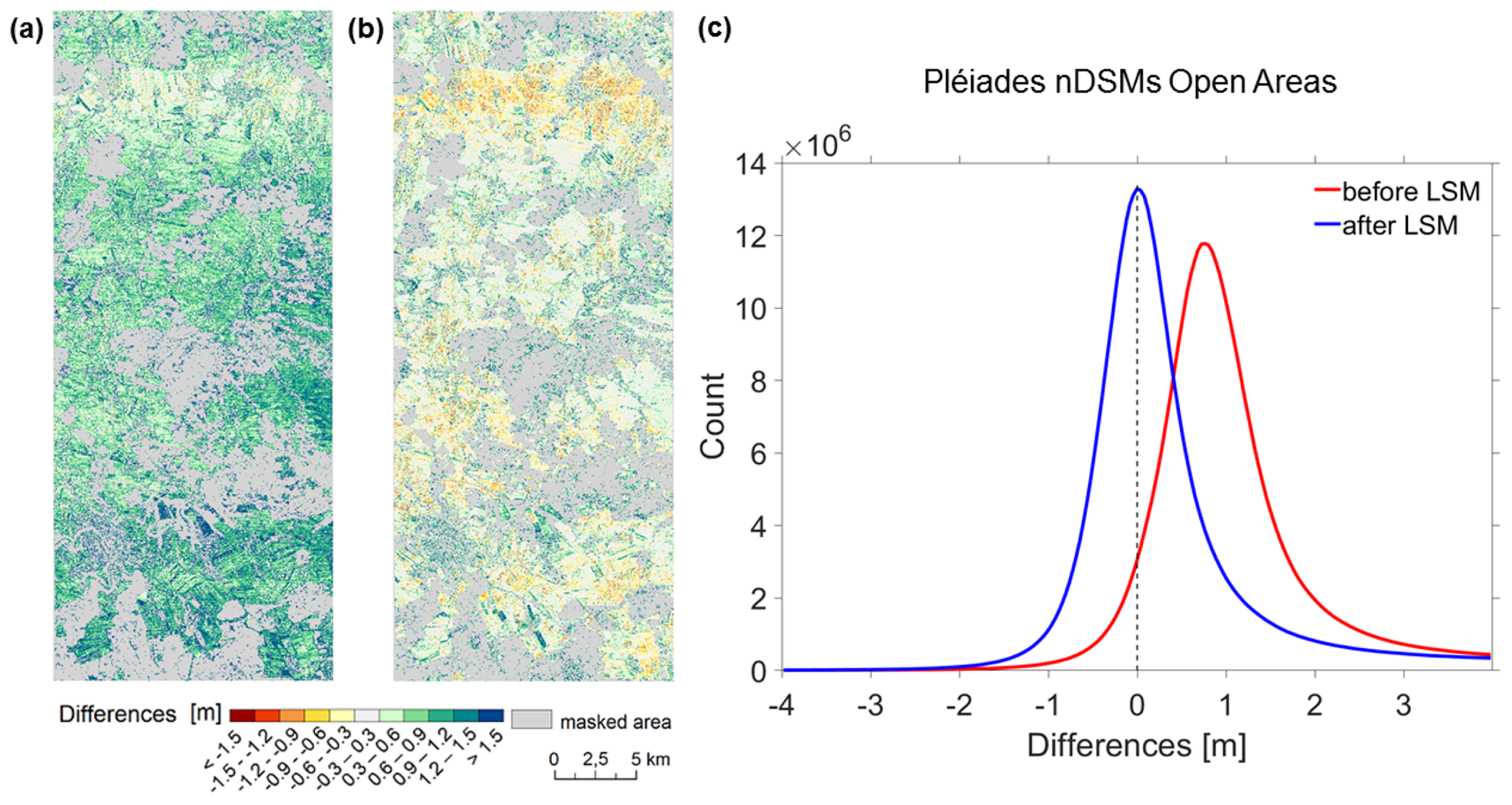
| CPs | 0.25 | 0.30 | 0.29 | 0.31 | 0.12 | 0.23 | 0.21 | 0.25 |
| DSM (open areas) | 0.80 | 0.53 | 0.51 | 0.96 | 0.15 | 0.60 | 0.50 | 0.61 |


Appendix B
| Predicted | ||||||
|---|---|---|---|---|---|---|
| Clutter | Roads | Buildings | Trees | Vehicles | ||
| Actual | Clutter | 11,588,872 | 614,421 | 0 | 9,309,164 | 0 |
| Roads | 463,755 | 21,421 | 0 | 422,481 | 0 | |
| Buildings | 106,155 | 279 | 0 | 29,155 | 0 | |
| Trees | 3,589,286 | 190,509 | 0 | 7,144,498 | 0 | |
| Vehicles | 1060 | 52 | 0 | 582 | 0 | |
| Predicted | ||||||
|---|---|---|---|---|---|---|
| Clutter | Roads | Buildings | Trees | Vehicles | ||
| Actual | Clutter | 53.87 | 2.86 | 0 | 43.27 | 0 |
| Roads | 51.09 | 2.36 | 0 | 46.55 | 0 | |
| Buildings | 78.29 | 0.21 | 0 | 21.50 | 0 | |
| Trees | 32.86 | 1.74 | 0 | 65.40 | 0 | |
| Vehicles | 62.57 | 3.07 | 0 | 34.36 | 0 | |
| Predicted | ||||||
|---|---|---|---|---|---|---|
| Clutter | Roads | Buildings | Trees | Vehicles | ||
| Actual | Clutter | 20,100,179 | 0 | 0 | 1,412,278 | 0 |
| Roads | 855,821 | 0 | 0 | 51,836 | 0 | |
| Buildings | 125,225 | 0 | 0 | 10,364 | 0 | |
| Trees | 10,218,858 | 0 | 0 | 705,435 | 0 | |
| Vehicles | 1623 | 0 | 0 | 71 | 0 | |
| Predicted | ||||||
|---|---|---|---|---|---|---|
| Clutter | Roads | Buildings | Trees | Vehicles | ||
| Actual | Clutter | 93.44 | 0 | 0 | 6.56 | 0 |
| Roads | 94.29 | 0 | 0 | 5.71 | 0 | |
| Buildings | 92.36 | 0 | 0 | 7.64 | 0 | |
| Trees | 93.54 | 0 | 0 | 6.46 | 0 | |
| Vehicles | 95.81 | 0 | 0 | 4.19 | 0 | |
| Predicted | ||||||
|---|---|---|---|---|---|---|
| Clutter | Roads | Buildings | Trees | Vehicles | ||
| Actual | Clutter | 10,804,589 | 417,105 | 61,491 | 4,367,882 | 869 |
| Roads | 727,020 | 32,852 | 10,115 | 271,748 | 48 | |
| Buildings | 22,370 | 1203 | 0 | 19,664 | 0 | |
| Trees | 9,958,478 | 456,497 | 63,983 | 6,264,999 | 777 | |
| Vehicles | 0 | 0 | 0 | 0 | 0 | |
| Predicted | ||||||
|---|---|---|---|---|---|---|
| Clutter | Roads | Buildings | Trees | Vehicles | ||
| Actual | Clutter | 50.22 | 3.38 | 0.10 | 46.29 | 0.00 |
| Roads | 45.95 | 3.62 | 0.13 | 50.29 | 0.00 | |
| Buildings | 45.35 | 7.46 | 0.00 | 47.19 | 0.00 | |
| Trees | 39.98 | 2.49 | 0.18 | 57.35 | 0.00 | |
| Vehicles | 51.30 | 2.83 | 0.00 | 45.87 | 0.00 | |
| Predicted | ||||||
|---|---|---|---|---|---|---|
| Clutter | Roads | Buildings | Trees | Vehicles | ||
| Actual | Clutter | 21,326,657 | 110,375 | 80,506 | 200,719 | 0 |
| Roads | 665,108 | 209,678 | 16,834 | 24,317 | 0 | |
| Buildings | 15,848 | 712 | 118,464 | 2012 | 0 | |
| Trees | 186,250 | 7460 | 2288 | 10,824,717 | 0 | |
| Vehicles | 1243 | 160 | 278 | 13 | 0 | |
| Predicted | ||||||
|---|---|---|---|---|---|---|
| Clutter | Roads | Buildings | Trees | Vehicles | ||
| Actual | Clutter | 98.20 | 0.51 | 0.37 | 0.92 | 0 |
| Roads | 72.62 | 22.89 | 1.84 | 2.65 | 0 | |
| Buildings | 11.56 | 0.52 | 86.45 | 1.47 | 0 | |
| Trees | 1.69 | 0.07 | 0.02 | 98.22 | 0 | |
| Vehicles | 73.38 | 9.45 | 16.41 | 0.77 | 0 | |
| Predicted | ||||||
|---|---|---|---|---|---|---|
| Clutter | Roads | Buildings | Trees | Vehicles | ||
| Actual | Clutter | 20,201,720 | 0 | 4883 | 1,306,322 | 0 |
| Roads | 775,555 | 0 | 587 | 131,538 | 0 | |
| Buildings | 6049 | 0 | 15,887 | 113,654 | 0 | |
| Trees | 1,292,805 | 0 | 15,870 | 9,615,985 | 0 | |
| Vehicles | 1181 | 0 | 2 | 511 | 0 | |
| Predicted | ||||||
|---|---|---|---|---|---|---|
| Clutter | Roads | Buildings | Trees | Vehicles | ||
| Actual | Clutter | 93.91 | 0 | 0.02 | 6.07 | 0 |
| Roads | 85.44 | 0 | 0.06 | 14.49 | 0 | |
| Buildings | 4.46 | 0 | 11.72 | 83.82 | 0 | |
| Trees | 11.83 | 0 | 0.15 | 88.02 | 0 | |
| Vehicles | 69.72 | 0 | 0.12 | 30.17 | 0 | |
| Predicted | ||||||
|---|---|---|---|---|---|---|
| Clutter | Roads | Buildings | Trees | Vehicles | ||
| Actual | Clutter | 20,610,793 | 223,248 | 38,686 | 640,198 | 0 |
| Roads | 657,941 | 224,697 | 9981 | 15,061 | 0 | |
| Buildings | 25,486 | 1027 | 107,293 | 1784 | 0 | |
| Trees | 661,638 | 3867 | 2274 | 10,256,881 | 0 | |
| Vehicles | 1049 | 522 | 109 | 14 | 0 | |
| Predicted | ||||||
|---|---|---|---|---|---|---|
| Clutter | Roads | Buildings | Trees | Vehicles | ||
| Actual | Clutter | 95.81 | 1.04 | 0.18 | 2.98 | 0 |
| Roads | 72.49 | 24.76 | 1.10 | 1.66 | 0 | |
| Buildings | 18.80 | 0.76 | 79.13 | 1.32 | 0 | |
| Trees | 6.06 | 0.04 | 0.02 | 93.89 | 0 | |
| Vehicles | 61.92 | 30.81 | 6.43 | 0.83 | 0 | |
| Predicted | ||||||
|---|---|---|---|---|---|---|
| Clutter | Roads | Buildings | Trees | Vehicles | ||
| Actual | Clutter | 13,627,522 | 615,499 | 106,489 | 4,793,811 | 1151 |
| Roads | 189,498 | 14,642 | 2471 | 23,374 | 232 | |
| Buildings | 13,721 | 572 | 213 | 17,642 | 0 | |
| Trees | 7,660,978 | 276,146 | 26,308 | 6,045,457 | 310 | |
| Vehicles | 20,738 | 798 | 108 | 44,009 | 1 | |
| Predicted | ||||||
|---|---|---|---|---|---|---|
| Clutter | Roads | Buildings | Trees | Vehicles | ||
| Actual | Clutter | 63.35 | 0.88 | 0.06 | 35.61 | 0.10 |
| Roads | 67.81 | 1.61 | 0.06 | 30.42 | 0.09 | |
| Buildings | 78.54 | 1.82 | 0.16 | 19.40 | 0.08 | |
| Trees | 43.88 | 0.21 | 0.16 | 55.34 | 0.40 | |
| Vehicles | 67.95 | 13.70 | 0.00 | 18.30 | 0.06 | |
Appendix C
Appendix D

References
- LeCun, Y.; Bengio, Y.; Hinton, G. Deep learning. Nature 2015, 521, 436. [Google Scholar] [CrossRef]
- Schmidhuber, J. Deep learning in neural networks: An overview. Neural Netw. 2015, 61, 85–117. [Google Scholar] [CrossRef] [Green Version]
- Jordan, M.I.; Mitchell, T.M. Machine learning: Trends, perspectives, and prospects. Science 2015, 349, 255–260. [Google Scholar] [CrossRef]
- Hirschberg, J.; Manning, C.D. Advances in natural language processing. Science 2015, 349, 261–266. [Google Scholar] [CrossRef]
- Bengio, Y.; Courville, A.; Vincent, P. Representation learning: A review and new perspectives. IEEE Trans. Pattern Anal. Mach. Intell. 2013, 35, 1798–1828. [Google Scholar] [CrossRef] [PubMed]
- Goodfellow, I.; Bengio, Y.; Courville, A. Deep Learning; MIT Press: Cambridge, MA, USA, 2016. [Google Scholar]
- Bengio, Y. Deep learning of representations for unsupervised and transfer learning. Proc. ICML Workshop Unsupervised Transf. Learn. 2012, 27, 17–36. [Google Scholar]
- Tshitoyan, V.; Dagdelen, J.; Weston, L.; Dunn, A.; Rong, Z.; Kononova, O.; Persson, K.A.; Ceder, G.; Jain, A. Unsupervised word embeddings capture latent knowledge from materials science literature. Nature 2019, 571, 95. [Google Scholar] [CrossRef] [PubMed] [Green Version]
- Devlin, J.; Chang, M.W.; Lee, K.; Toutanova, K. Bert: Pre-training of deep bidirectional transformers for language understanding. arXiv 2018, arXiv:1810.04805. [Google Scholar]
- Liu, Y.; Ott, M.; Goyal, N.; Du, J.; Joshi, M.; Chen, D.; Levy, O.; Lewis, M.; Zettlemoyer, L.; Stoyanov, V. RoBERTa: A Robustly Optimized BERT Pretraining Approach. arXiv 2019, arXiv:1907.11692. [Google Scholar]
- Howard, J.; Ruder, S. Universal Language Model Fine-tuning for Text Classification. arXiv 2018, arXiv:1801.06146, 328–339. [Google Scholar]
- Krizhevsky, A.; Sutskever, I.; Hinton, G.E. ImageNet Classification with Deep Convolutional Neural Networks. In Advances in Neural Information Processing Systems 25; Pereira, F., Burges, C.J.C., Bottou, L., Weinberger, K.Q., Eds.; Curran Associates, Inc.: New York, NY, USA, 2012; pp. 1097–1105. [Google Scholar]
- Huang, Y.; Cheng, Y.; Chen, D.; Lee, H.; Ngiam, J.; Le, Q.V.; Chen, Z. Gpipe: Efficient training of giant neural networks using pipeline parallelism. arXiv 2018, arXiv:1811.06965. [Google Scholar]
- Redmon, J.; Divvala, S.; Girshick, R.; Farhadi, A. You only look once: Unified, real-time object detection. In Proceedings of the IEEE Conference on Computer Vision and Pattern Recognition, Las Vegas, NV, USA, 26 June–1 July 2016; pp. 779–788. [Google Scholar]
- Redmon, J.; Farhadi, A. YOLO9000: Better, faster, stronger. In Proceedings of the IEEE Conference on Computer Vision and Pattern Recognition, Honolulu, HI, USA, 21–26 July 2017; pp. 7263–7271. [Google Scholar]
- Redmon, J.; Farhadi, A. Yolov3: An incremental improvement. arXiv 2018, arXiv:1804.02767. [Google Scholar]
- Sauer, A.; Aljalbout, E.; Haddadin, S. Tracking Holistic Object Representations. arXiv 2019, arXiv:1907.12920. [Google Scholar]
- Moon, G.; Chang, J.; Lee, K.M. Camera Distance-aware Top-down Approach for 3D Multi-person Pose Estimation from a Single RGB Image. In Proceedings of the IEEE Conference on International Conference on Computer Vision (ICCV), Long Beach, CA, USA, 16–20 June 2019. [Google Scholar]
- Kocabas, M.; Karagoz, S.; Akbas, E. Multiposenet: Fast multi-person pose estimation using pose residual network. In Proceedings of the European Conference on Computer Vision (ECCV), Munich, Germany, 8–14 September 2018; pp. 417–433. [Google Scholar]
- Lugaresi, C.; Tang, J.; Nash, H.; McClanahan, C.; Uboweja, E.; Hays, M.; Zhang, F.; Chang, C.L.; Yong, M.G.; Lee, J.; et al. MediaPipe: A Framework for Building Perception Pipelines. arXiv 2019, arXiv:1906.08172. [Google Scholar]
- Dapogny, A.; Bailly, K.; Cord, M. DeCaFA: Deep Convolutional Cascade for Face Alignment in the Wild. arXiv 2019, arXiv:1904.02549. [Google Scholar]
- Wang, Z.; Chen, J.; Hoi, S.C. Deep learning for image super-resolution: A survey. arXiv 2019, arXiv:1902.06068. [Google Scholar]
- Liu, C.; Chen, L.C.; Schroff, F.; Adam, H.; Hua, W.; Yuille, A.L.; Fei-Fei, L. Auto-deeplab: Hierarchical neural architecture search for semantic image segmentation. In Proceedings of the IEEE Conference on Computer Vision and Pattern Recognition, Long Beach, CA, USA, 15–21 June 2019; pp. 82–92. [Google Scholar]
- Chen, L.C.; Papandreou, G.; Kokkinos, I.; Murphy, K.; Yuille, A.L. Deeplab: Semantic image segmentation with deep convolutional nets, atrous convolution, and fully connected crfs. IEEE Trans. Pattern Anal. Mach. Intell. 2017, 40, 834–848. [Google Scholar]
- Voulodimos, A.; Doulamis, N.; Doulamis, A.; Protopapadakis, E. Deep learning for computer vision: A brief review. Comput. Intell. Neurosci. 2018, 2018, 7068349. [Google Scholar]
- Badrinarayanan, V.; Kendall, A.; Cipolla, R. Segnet: A deep convolutional encoder-decoder architecture for image segmentation. IEEE Trans. Pattern Anal. Mach. Intell. 2017, 39, 2481–2495. [Google Scholar]
- Vu, T.H.; Jain, H.; Bucher, M.; Cord, M.; Pérez, P. DADA: Depth-aware Domain Adaptation in Semantic Segmentation. In Proceedings of the IEEE International Conference on Computer Vision, Soul, Korea, 27 October–2 November 2019. [Google Scholar]
- Chen, L.C.; Zhu, Y.; Papandreou, G.; Schroff, F.; Adam, H. Encoder-Decoder with Atrous Separable Convolution for Semantic Image Segmentation. In Proceedings of the European Conference on Computer Vision (ECCV), Munich, Germany, 8–14 September 2018. [Google Scholar]
- Schmidt, J.; Marques, M.R.; Botti, S.; Marques, M.A. Recent advances and applications of machine learning in solid-state materials science. npj Comput. Mater. 2019, 5, 1–36. [Google Scholar]
- Butler, K.T.; Davies, D.W.; Cartwright, H.; Isayev, O.; Walsh, A. Machine learning for molecular and materials science. Nature 2018, 559, 547. [Google Scholar]
- Wimmers, A.; Velden, C.; Cossuth, J.H. Using Deep Learning to Estimate Tropical Cyclone Intensity from Satellite Passive Microwave Imagery. Mon. Weather Rev. 2019, 147, 2261–2282. [Google Scholar]
- Topol, E.J. High-performance medicine: The convergence of human and artificial intelligence. Nat. Med. 2019, 25, 44. [Google Scholar]
- Esteva, A.; Robicquet, A.; Ramsundar, B.; Kuleshov, V.; DePristo, M.; Chou, K.; Cui, C.; Corrado, G.; Thrun, S.; Dean, J. A guide to deep learning in healthcare. Nat. Med. 2019, 25, 24. [Google Scholar]
- Chen, P.; Gadepalli, K.; MacDonald, R.; Liu, Y.; Kadowaki, S.; Nagpal, K.; Kohlberger, T.; Dean, J.; Corrado, G.S.; Hipp, J.D.; et al. An augmented reality microscope with real-time artificial intelligence integration for cancer diagnosis. Nat. Med. 2019, 25, 1453–1457. [Google Scholar]
- Esteva, A.; Kuprel, B.; Novoa, R.A.; Ko, J.; Swetter, S.M.; Blau, H.M.; Thrun, S. Dermatologist-level classification of skin cancer with deep neural networks. Nature 2017, 542, 115. [Google Scholar]
- Porumb, M.; Iadanza, E.; Massaro, S.; Pecchia, L. A convolutional neural network approach to detect congestive heart failure. Biomed. Signal Process. Control 2020, 55, 101597. [Google Scholar]
- Avati, A.; Jung, K.; Harman, S.; Downing, L.; Ng, A.; Shah, N.H. Improving palliative care with deep learning. BMC Med. Inform. Decis. Mak. 2018, 18, 122. [Google Scholar]
- Siddiquee, M.M.R.; Zhou, Z.; Tajbakhsh, N.; Feng, R.; Gotway, M.B.; Bengio, Y.; Liang, J. Learning Fixed Points in Generative Adversarial Networks: From Image-to-Image Translation to Disease Detection and Localization. In Proceedings of the IEEE International Conference on Computer Vision, Soul, Korea, 27 October–2 November 2019. [Google Scholar]
- Wiens, J.; Saria, S.; Sendak, M.; Ghassemi, M.; Liu, V.X.; Doshi-Velez, F.; Jung, K.; Heller, K.; Kale, D.; Saeed, M.; et al. Do no harm: A roadmap for responsible machine learning for health care. Nat. Med. 2019, 25, 1337–1340. [Google Scholar]
- DeVries, P.M.; Viégas, F.; Wattenberg, M.; Meade, B.J. Deep learning of aftershock patterns following large earthquakes. Nature 2018, 560, 632. [Google Scholar]
- Kong, Q.; Trugman, D.T.; Ross, Z.E.; Bianco, M.J.; Meade, B.J.; Gerstoft, P. Machine learning in seismology: Turning data into insights. Seismol. Res. Lett. 2018, 90, 3–14. [Google Scholar]
- Ross, Z.E.; Meier, M.A.; Hauksson, E.; Heaton, T.H. Generalized seismic phase detection with deep learning. Bull. Seismol. Soc. Am. 2018, 108, 2894–2901. [Google Scholar]
- Senior, A.; Evans, R.; Jumper, J.; Kirkpatrick, J.; Sifre, L.; Green, T.; Qin, C.; Zidek, A.; Nelson, A.; Bridgland, A.; et al. Improved protein structure prediction using potentials from deep learning. Nature 2020, 577, 706–710. [Google Scholar]
- Moen, E.; Bannon, D.; Kudo, T.; Graf, W.; Covert, M.; Van Valen, D. Deep learning for cellular image analysis. Nat. Methods 2019, 16, 1233–1246. [Google Scholar]
- Goh, G.B.; Hodas, N.O.; Vishnu, A. Deep learning for computational chemistry. J. Comput. Chem. 2017, 38, 1291–1307. [Google Scholar]
- Baldi, P.; Sadowski, P.; Whiteson, D. Searching for exotic particles in high-energy physics with deep learning. Nat. Commun. 2014, 5, 4308. [Google Scholar]
- Tacchino, F.; Macchiavello, C.; Gerace, D.; Bajoni, D. An artificial neuron implemented on an actual quantum processor. npj Quantum Inf. 2019, 5, 26. [Google Scholar]
- Xie, Y.; Franz, E.; Chu, M.; Thuerey, N. tempoGAN: A Temporally Coherent, Volumetric GAN for Super-resolution Fluid Flow. ACM Trans. Graph. (TOG) 2018, 37, 95. [Google Scholar]
- Mrowca, D.; Zhuang, C.; Wang, E.; Haber, N.; Fei-Fei, L.F.; Tenenbaum, J.; Yamins, D.L. Flexible neural representation for physics prediction. In Proceedings of the Advances in Neural Information Processing Systems, Montréal, QC, Canada, 3–8 December 2018; pp. 8799–8810. [Google Scholar]
- Lutter, M.; Ritter, C.; Peters, J. International Conference on Learning Representations Learning. arXiv 2019, arXiv:1907.04490. [Google Scholar]
- Goy, A.; Arthur, K.; Li, S.; Barbastathis, G. Low photon count phase retrieval using deep learning. Phys. Rev. Lett. 2018, 121, 243902. [Google Scholar]
- Guest, D.; Cranmer, K.; Whiteson, D. Deep learning and its application to LHC physics. Annu. Rev. Nucl. Part. Sci. 2018, 68, 161–181. [Google Scholar]
- Kutz, J.N. Deep learning in fluid dynamics. J. Fluid Mech. 2017, 814, 1–4. [Google Scholar]
- Ferreira, B.Q.; Baía, L.; Faria, J.; Sousa, R.G. A Unified Model with Structured Output for Fashion Images Classification. arXiv 2018, arXiv:1907.04490. [Google Scholar]
- Hsiao, W.L.; Grauman, K. Learning the Latent “Look”: Unsupervised Discovery of a Style-Coherent Embedding from Fashion Images. In Proceedings of the International Conference on Computer Vision (ICCV), Venice, Italy, 22–29 October 2017. [Google Scholar]
- Liu, Z.; Luo, P.; Qiu, S.; Wang, X.; Tang, X. DeepFashion: Powering Robust Clothes Recognition and Retrieval with Rich Annotations. In Proceedings of the Conference on Computer Vision and Pattern Recognition (CVPR), Las Vegas, NV, USA, 27–30 June 2016; pp. 1096–1104. [Google Scholar]
- Ma, L.; Liu, Y.; Zhang, X.; Ye, Y.; Yin, G.; Johnson, B.A. Deep learning in remote sensing applications: A meta-analysis and review. ISPRS J. Photogramm. Remote. Sens. 2019, 152, 166–177. [Google Scholar]
- Zhu, X.X.; Tuia, D.; Mou, L.; Xia, G.S.; Zhang, L.; Xu, F.; Fraundorfer, F. Deep learning in remote sensing: A comprehensive review and list of resources. IEEE Geosci. Remote Sens. Mag. 2017, 5, 8–36. [Google Scholar]
- Zhang, L.; Zhang, L.; Du, B. Deep learning for remote sensing data: A technical tutorial on the state of the art. IEEE Geosci. Remote Sens. Mag. 2016, 4, 22–40. [Google Scholar]
- Qi, C.R.; Su, H.; Mo, K.; Guibas, L.J. Pointnet: Deep learning on point sets for 3d classification and segmentation. In Proceedings of the IEEE Conference on Computer Vision and Pattern Recognition, Honolulu, HI, USA, 21–26 July 2017; pp. 652–660. [Google Scholar]
- Graham, B.; Engelcke, M.; van der Maaten, L. 3D Semantic Segmentation With Submanifold Sparse Convolutional Networks. In Proceedings of the IEEE Conference on Computer Vision and Pattern Recognition (CVPR), Salt Lake City, UT, USA, 18–22 June 2018. [Google Scholar]
- Winiwarter, L.; Mandlburger, G.; Schmohl, S.; Pfeifer, N. Classification of ALS Point Clouds Using End-to-End Deep Learning. PFG J. Photogramm. Remote Sens. Geoinf. Sci. 2019, 87, 75–90. [Google Scholar] [CrossRef]
- Stubbings, P.; Peskett, J.; Rowe, F.; Arribas-Bel, D. A Hierarchical Urban Forest Index Using Street-Level Imagery and Deep Learning. Remote Sens. 2019, 11, 1395. [Google Scholar]
- He, J.; Li, X.; Yao, Y.; Hong, Y.; Jinbao, Z. Mining transition rules of cellular automata for simulating urban expansion by using the deep learning techniques. Int. J. Geogr. Inf. Sci. 2018, 32, 2076–2097. [Google Scholar]
- Madu, C.N.; Kuei, C.h.; Lee, P. Urban sustainability management: A deep learning perspective. Sustain. Cities Soc. 2017, 30, 1–17. [Google Scholar]
- Zhou, K.; Ming, D.; Lv, X.; Fang, J. CNN-based Land Cover Classification Combining Stratified Segmentation and Fusion of Point Cloud and Very High-Spatial Resolution Remote Sensing Image Data. Remote Sens. 2019, 11, 2065. [Google Scholar]
- Dyson, J.; Mancini, A.; Frontoni, E.; Zingaretti, P. Deep Learning for Soil and Crop Segmentation from Remotely Sensed Data. Remote Sen. 2019, 11, 1859. [Google Scholar]
- Kussul, N.; Lavreniuk, M.; Skakun, S.; Shelestov, A. Deep learning classification of land cover and crop types using remote sensing data. IEEE Geosci. Remote Sens. Lett. 2017, 14, 778–782. [Google Scholar]
- Kamilaris, A.; Prenafeta-Boldú, F.X. Deep learning in agriculture: A survey. Comput. Electron. Agric. 2018, 147, 70–90. [Google Scholar]
- Weiss, M.; Jacob, F.; Duveiller, G. Remote sensing for agricultural applications: A meta-review. Remote Sens. Environ. 2020, 236, 111402. [Google Scholar]
- Lambers, K.; Verschoof-van der Vaart, W.B.; Bourgeois, Q.P. Integrating Remote Sensing, Machine Learning, and Citizen Science in Dutch Archaeological Prospection. Remote Sens. 2019, 11, 794. [Google Scholar]
- Ajami, A.; Kuffer, M.; Persello, C.; Pfeffer, K. Identifying a Slums’ Degree of Deprivation from VHR Images Using Convolutional Neural Networks. Remote Sens. 2019, 11, 1282. [Google Scholar]
- Wurm, M.; Stark, T.; Zhu, X.X.; Weigand, M.; Taubenböck, H. Semantic segmentation of slums in satellite images using transfer learning on fully convolutional neural networks. ISPRS J. Photogramm. Remote Sens. 2019, 150, 59–69. [Google Scholar]
- Jean, N.; Burke, M.; Xie, M.; Davis, W.M.; Lobell, D.B.; Ermon, S. Combining satellite imagery and machine learning to predict poverty. Science 2016, 353, 790–794. [Google Scholar]
- Grinias, I.; Panagiotakis, C.; Tziritas, G. MRF-based segmentation and unsupervised classification for building and road detection in peri-urban areas of high-resolution satellite images. ISPRS J. Photogramm. Remote Sens. 2016, 122, 145–166. [Google Scholar]
- Montoya-Zegarra, J.A.; Wegner, J.D.; Ladickỳ, L.; Schindler, K. Semantic segmentation of aerial images in urban areas with class-specific higher-order cliques. ISPRS Ann. Photogramm. Remote Sens. Spat. Inf. Sci. 2015, 2, 127. [Google Scholar]
- Dumas, M.; La Rosa, M.; Mendling, J.; Reijers, H.A. Fundamentals of Business Process Management, 2nd ed.; Springer: Berlin/Heidelberg, Germany, 2018. [Google Scholar]
- Cabanillas, C.; Di Ciccio, C.; Mendling, J.; Baumgrass, A. Predictive Task Monitoring for Business Processes. In International Conference on Business Process Management; Springer: Berlin/Heidelberg, Germany, 2014; pp. 424–432. [Google Scholar]
- Satyal, S.; Weber, I.; young Paik, H.; Ciccio, C.D.; Mendling, J. Business process improvement with the AB-BPM methodology. Inf. Syst. 2019, 84, 283–298. [Google Scholar]
- Weidlich, M.; Polyvyanyy, A.; Desai, N.; Mendling, J.; Weske, M. Process compliance analysis based on behavioural profiles. Inf. Syst. 2011, 36, 1009–1025. [Google Scholar]
- Mannhardt, F.; de Leoni, M.; Reijers, H.A.; van der Aalst, W.M.P. Balanced multi-perspective checking of process conformance. Computing 2016, 98, 407–437. [Google Scholar]
- Rozinat, A.; Van der Aalst, W.M. Conformance testing: Measuring the fit and appropriateness of event logs and process models. In BPM; Springer: Berlin/Heidelberg, Germany, 2005; pp. 163–176. [Google Scholar]
- Van Der Aalst, W.; Adriansyah, A.; De Medeiros, A.K.A.; Arcieri, F.; Baier, T.; Blickle, T.; Bose, J.C.; Van Den Brand, P.; Brandtjen, R.; Buijs, J.; et al. Process mining manifesto. In BPM; Springer: Berlin/Heidelberg, Germany, 2011; pp. 169–194. [Google Scholar]
- Klinkmüller, C.; Ponomarev, A.; Tran, A.B.; Weber, I.; van der Aalst, W. Mining Blockchain Processes: Extracting Process Mining Data from Blockchain Applications. In International Conference on Business Process Management; Springer: Berlin/Heidelberg, Germany, 2019; pp. 71–86. [Google Scholar]
- Mühlberger, R.; Bachhofner, S.; Di Ciccio, C.; García-Bañuelos, L.; López-Pintado, O. Extracting Event Logs for Process Mining from Data Stored on the Blockchain. In Business Process Management Workshops; Springer: Berlin/Heidelberg, Germany, 2019. [Google Scholar]
- Klinkmüller, C.; Müller, R.; Weber, I. Mining Process Mining Practices: An Exploratory Characterization of Information Needs in Process Analytics. In International Conference on Business Process Management; Springer: Berlin/Heidelberg, Germany, 2019; pp. 322–337. [Google Scholar]
- Del-Río-Ortega, A.; Resinas, M.; Cabanillas, C.; Ruiz-Cortés, A. On the definition and design-time analysis of process performance indicators. Inf. Syst. 2013, 38, 470–490. [Google Scholar]
- Kis, I.; Bachhofner, S.; Di Ciccio, C.; Mendling, J. Towards a data-driven framework for measuring process performance. In Enterprise, Business-Process and Information Systems Modeling; Springer: Berlin/Heidelberg, Germany, 2017; pp. 3–18. [Google Scholar]
- Bachhofner, S.; Kis, I.; Di Ciccio, C.; Mendling, J. Towards a Multi-parametric Visualisation Approach for Business Process Analytics. In Proceedings of the Advanced Information Systems Engineering Workshops, Essen, Germany, 12–16 June 2017; pp. 85–91. [Google Scholar]
- Long, J.; Shelhamer, E.; Darrell, T. Fully convolutional networks for semantic segmentation. In Proceedings of the IEEE Conference on Computer Vision and Pattern Recognition, Boston, MA, USA, 7–12 June 2015; pp. 3431–3440. [Google Scholar]
- Choy, C.; Gwak, J.; Savarese, S. 4D Spatio Temporal ConvNet: Minkowski Convolutional Neural Networks. In Proceedings of the IEEE Conference on Computer Vision and Pattern Recognition, Long Beach, CA, USA, 15–21 June 2019. [Google Scholar]
- Ronneberger, O.; Fischer, P.; Brox, T. U-net: Convolutional networks for biomedical image segmentation. In International Conference on Medical Image Computing and Computer-Assisted Intervention; Springer: Berlin/Heidelberg, Germany, 2015; pp. 234–241. [Google Scholar]
- He, K.; Zhang, X.; Ren, S.; Sun, J. Deep residual learning for image recognition. In Proceedings of the IEEE Conference on Computer Vision and Pattern Recognition, Las Vegas, NV, USA, 26 June–1 July 2016; pp. 770–778. [Google Scholar]
- Glorot, X.; Bordes, A.; Bengio, Y. Deep sparse rectifier neural networks. In Proceedings of the Fourteenth International Conference on Artificial Intelligence and Statistics, Ft. Lauderdale, FL, USA, 22–23 April 2011; pp. 315–323. [Google Scholar]
- Dahl, G.E.; Sainath, T.N.; Hinton, G.E. Improving deep neural networks for LVCSR using rectified linear units and dropout. In Proceedings of the 2013 IEEE International Conference on Acoustics, Speech and Signal Processing, Vancouver, BC, Canada, 26–31 May 2013; pp. 8609–8613. [Google Scholar]
- Ioffe, S.; Szegedy, C. Batch normalization: Accelerating deep network training by reducing internal covariate shift. arXiv 2015, arXiv:1502.03167. [Google Scholar]
- Bjorck, N.; Gomes, C.P.; Selman, B.; Weinberger, K.Q. Understanding batch normalization. In Proceedings of the Advances in Neural Information Processing Systems, Montréal, QC, Canada, 3–8 December 2018; pp. 7694–7705. [Google Scholar]
- Waldhauser, C.; Hochreiter, R.; Otepka, J.; Pfeifer, N.; Ghuffar, S.; Korzeniowska, K.; Wagner, G. Automated classification of airborne laser scanning point clouds. In Solving Computationally Expensive Engineering Problems; Springer: Berlin/Heidelberg, Germany, 2014; pp. 269–292. [Google Scholar]
- Goutte, C.; Gaussier, E. A probabilistic interpretation of precision, recall and F-score, with implication for evaluation. In European Conference on Information Retrieval; Springer: Berlin/Heidelberg, Germany, 2005; pp. 345–359. [Google Scholar]
- Zhang, D.; Wang, J.; Zhao, X. Estimating the uncertainty of average F1 scores. In Proceedings of the 2015 International Conference on the Theory of Information Retrieval, New York, NY, USA, 27–30 September 2015; pp. 317–320. [Google Scholar]
- Yue, Y.; Finley, T.; Radlinski, F.; Joachims, T. A support vector method for optimizing average precision. In Proceedings of the 30th Annual International ACM SIGIR Conference on Research and Development in Information Retrieval, New York, NY, USA, 23–27 July 2007; pp. 271–278. [Google Scholar]
- Cohen, J. A coefficient of agreement for nominal scales. Educ. Psychol. Meas. 1960, 20, 37–46. [Google Scholar]
- Plaza-Leiva, V.; Gomez-Ruiz, J.A.; Mandow, A.; García-Cerezo, A. Voxel-based neighborhood for spatial shape pattern classification of lidar point clouds with supervised learning. Sensors 2017, 17, 594. [Google Scholar]
- Jurman, G.; Riccadonna, S.; Furlanello, C. A comparison of MCC and CEN error measures in multi-class prediction. PLoS ONE 2012, 7, e41882. [Google Scholar]
- Paszke, A.; Gross, S.; Chintala, S.; Chanan, G.; Yang, E.; DeVito, Z.; Lin, Z.; Desmaison, A.; Antiga, L.; Lerer, A. Automatic Differentiation in PyTorch. In Proceedings of the Neural Information Processing Systems, Long Beach, CA, USA, 4–9 December 2017. [Google Scholar]
- Jia, Y.; Shelhamer, E.; Donahue, J.; Karayev, S.; Long, J.; Girshick, R.; Guadarrama, S.; Darrell, T. Caffe: Convolutional Architecture for Fast Feature Embedding. In Proceedings of the 22nd ACM International Conference on Multimedia, Orlando, FL, USA, 3–7 November 2014; pp. 675–678. [Google Scholar]
- R Core Team. R: A Language and Environment for Statistical Computing; R Foundation for Statistical Computing: Vienna, Austria, 2018. [Google Scholar]
- Pfeifer, N.; Mandlburger, G.; Otepka, J.; Karel, W. OPALS—A framework for Airborne Laser Scanning data analysis. Comput. Environ. Urban Syst. 2014, 45, 125–136. [Google Scholar]
- Trimble. Match-T DSM Reference Manual; Trimble, Inc.: Sunnyvale, CA, USA, 2016. [Google Scholar]
- Trimble Geospatial. Available online: http://www.inpho.de (accessed on 7 March 2019).
- Hu, F.; Xia, G.S.; Hu, J.; Zhang, L. Transferring deep convolutional neural networks for the scene classification of high-resolution remote sensing imagery. Remote Sens. 2015, 7, 14680–14707. [Google Scholar]
- Sun, Y.; Tian, Y.; Xu, Y. Problems of encoder-decoder frameworks for high-resolution remote sensing image segmentation: Structural stereotype and insufficient learning. Neurocomputing 2019, 330, 297–304. [Google Scholar]
- Bischke, B.; Helber, P.; Folz, J.; Borth, D.; Dengel, A. Multi-Task Learning for Segmentation of Building Footprints with Deep Neural Networks. arXiv 2017, arXiv:1709.05932. [Google Scholar]
- Yi, Y.; Zhang, Z.; Zhang, W.; Zhang, C.; Li, W.; Zhao, T. Semantic Segmentation of Urban Buildings from VHR Remote Sensing Imagery Using a Deep Convolutional Neural Network. Remote Sens. 2019, 11, 1774. [Google Scholar]
- Guo, Z.; Wu, G.; Song, X.; Yuan, W.; Chen, Q.; Zhang, H.; Shi, X.; Xu, M.; Xu, Y.; Shibasaki, R.; et al. Super-Resolution Integrated Building Semantic Segmentation for Multi-Source Remote Sensing Imagery. IEEE Access 2019, 7, 99381–99397. [Google Scholar]
- Eerapu, K.K.; Ashwath, B.; Lal, S.; Dell’acqua, F.; Dhan, A.N. Dense Refinement Residual Network for Road Extraction from Aerial Imagery Data. IEEE Access 2019, 7, 151764–151782. [Google Scholar]
- Marmanis, D.; Wegner, J.D.; Galliani, S.; Schindler, K.; Datcu, M.; Stilla, U. Semantic segmentation of aerial images with an ensemble of CNNs. ISPRS Ann. Photogramm. Remote Sens. Spat. Inf. Sci. 2016, 3, 473. [Google Scholar]
- Li, Y.; Zhang, H.; Shen, Q. Spectral–spatial classification of hyperspectral imagery with 3D convolutional neural network. Remote Sens. 2017, 9, 67. [Google Scholar]
- Sellami, A.; Farah, M.; Farah, I.R.; Solaiman, B. Hyperspectral imagery classification based on semi-supervised 3-D deep neural network and adaptive band selection. Expert Syst. Appl. 2019, 129, 246–259. [Google Scholar]
- Yu, X.; Hyyppä, J.; Vastaranta, M.; Holopainen, M.; Viitala, R. Predicting individual tree attributes from airborne laser point clouds based on the random forests technique. ISPRS J. Photogramm. Remote. Sens. 2011, 66, 28–37. [Google Scholar]
- Otepka, J.; Ghuffar, S.; Waldhauser, C.; Hochreiter, R.; Pfeifer, N. Georeferenced point clouds: A survey of features and point cloud management. ISPRS Int. J. Geo-Inf. 2013, 2, 1038–1065. [Google Scholar]
- Zhou, Y.; Tuzel, O. Voxelnet: End-to-end learning for point cloud based 3d object detection. In Proceedings of the IEEE Conference on Computer Vision and Pattern Recognition, Salt Lake City, UT, USA, 18–22 June 2018; pp. 4490–4499. [Google Scholar]
- Hua, B.S.; Tran, M.K.; Yeung, S.K. Pointwise convolutional neural networks. In Proceedings of the IEEE Conference on Computer Vision and Pattern Recognition, Salt Lake City, UT, USA, 18–22 June 2018; pp. 984–993. [Google Scholar]
- Vo, A.V.; Truong-Hong, L.; Laefer, D.F.; Tiede, D.; d’Oleire Oltmanns, S.; Baraldi, A.; Shimoni, M.; Moser, G.; Tuia, D. Processing of extremely high resolution LiDAR and RGB data: Outcome of the 2015 IEEE GRSS data fusion contest—Part B: 3-D contest. IEEE J. Sel. Top. Appl. Earth Obs. Remote Sens. 2016, 9, 5560–5575. [Google Scholar]
- Vo, A.V.; Truong-Hong, L.; Laefer, D.F. Aerial laser scanning and imagery data fusion for road detection in city scale. In Proceedings of the 2015 IEEE International Geoscience and Remote Sensing Symposium (IGARSS), Milano, Italy, 26–31 July 201; pp. 4177–4180.
- Maxwell, A.E.; Warner, T.A.; Fang, F. Implementation of machine-learning classification in remote sensing: An applied review. Int. J. Remote Sens. 2018, 39, 2784–2817. [Google Scholar]
- Kaelbling, L.P.; Littman, M.L.; Moore, A.W. Reinforcement learning: A survey. J. Artif. Intell. Res. 1996, 4, 237–285. [Google Scholar]
- Silver, D.; Huang, A.; Maddison, C.J.; Guez, A.; Sifre, L.; Van Den Driessche, G.; Schrittwieser, J.; Antonoglou, I.; Panneershelvam, V.; Lanctot, M.; et al. Mastering the game of Go with deep neural networks and tree search. Nature 2016, 529, 484. [Google Scholar]
- Nadell, C.C.; Huang, B.; Malof, J.M.; Padilla, W.J. Deep learning for accelerated all-dielectric metasurface design. Opt. Express 2019, 27, 27523–27535. [Google Scholar]
- Stokes, J.M.; Yang, K.; Swanson, K.; Jin, W.; Cubillos-Ruiz, A.; Donghia, N.M.; MacNair, C.R.; French, S.; Carfrae, L.A.; Bloom-Ackerman, Z.; et al. A Deep Learning Approach to Antibiotic Discovery. Cell 2020, 180, 688–702. [Google Scholar]
- Lipton, Z.C.; Steinhardt, J. Troubling trends in machine learning scholarship. arXiv 2018, arXiv:1807.03341. [Google Scholar]
- Gundersen, O.E.; Kjensmo, S. State of the art: Reproducibility in artificial intelligence. In Proceedings of the Thirty-Second AAAI Conference on Artificial Intelligence, New Orleans, LO, USA, 2–7 February 2018. [Google Scholar]
- Gibney, E. This AI researcher is trying to ward off a reproducibility crisis. Nature 2019, 577, 14. [Google Scholar]
- Ferrari Dacrema, M.; Cremonesi, P.; Jannach, D. Are We Really Making Much Progress? A Worrying Analysis of Recent Neural Recommendation Approaches. In Proceedings of the 13th ACM Conference on Recommender Systems (RecSys 2019), Copenhagen, Denmark, 16–20 September 2019. [Google Scholar]
- Fu, W.; Menzies, T. Easy over hard: A case study on deep learning. In Proceedings of the 2017 11th Joint Meeting on Foundations of Software Engineering, Paderborn, Germany, 4–8 September 2017; pp. 49–60. [Google Scholar]
- Baker, M. Over half of psychology studies fail reproducibility test. Nat. News 2015. Available online: https://0-www-nature-com.brum.beds.ac.uk/news/over-half-of-psychology-studies-fail-reproducibility-test-1.18248 (accessed on 7 April 2020). [CrossRef]
- Baker, M. 1,500 scientists lift the lid on reproducibility. Nat. News 2016, 533, 452. [Google Scholar] [CrossRef] [PubMed] [Green Version]
- Gannot, G.; Cutting, M.A.; Fischer, D.J.; Hsu, L.J. Reproducibility and transparency in biomedical sciences. Oral Dis. 2017, 23, 813. [Google Scholar]
- Goodman, S.N.; Fanelli, D.; Ioannidis, J.P. What does research reproducibility mean? Sci. Transl. Med. 2016, 8, 341ps12. [Google Scholar]
- Nuzzo, R. How scientists fool themselves–and how they can stop. Nat. News 2015, 526, 182. [Google Scholar]
- Menke, J.; Roelandse, M.; Ozyurt, B.; Martone, M.; Bandrowski, A. Rigor and Transparency Index, a new metric of quality for assessing biological and medical science methods. bioRxiv 2020. [Google Scholar] [CrossRef] [Green Version]
- Chawla, D.S. Software Searches out Reproducibility Issues in Scientific Papers. 2020. Available online: https://0-www-nature-com.brum.beds.ac.uk/articles/d41586-020-00104-6 (accessed on 7 April 2020).
- Breiman, L. Classification and Regression Trees; Routledge: Abingdon-on-Thames, UK, 2017. [Google Scholar]
- Weinmann, M.; Jutzi, B.; Mallet, C. Feature relevance assessment for the semantic interpretation of 3D point cloud data. ISPRS Ann. Photogramm. Remote Sens. Spat. Inf. Sci. 2013, 5, 1. [Google Scholar]
- Dai, A.; Chang, A.X.; Savva, M.; Halber, M.; Funkhouser, T.; Nießner, M. ScanNet: Richly-annotated 3D Reconstructions of Indoor Scenes. In Proceedings of the IEEE Computer Vision and Pattern Recognition (CVPR), Honolulu, HI, USA, 21–26 July 2017. [Google Scholar]
- Tieleman, T.; Hinton, G. Lecture 6.5-rmsprop: Divide the gradient by a running average of its recent magnitude. COURSERA Neural Netw. Mach. Learn. 2012, 4, 26–31. [Google Scholar]
- Ressl, C.; Mandlburger, G.; Pfeifer, N. Investigating Adjustment of Airborne Laser Scanning Strips without Usage of GNSS/IMU Trajectory Data. In Proceedings of the ISPRS Workshop Laserscanning 09, Paris, France, 1–2 September 2009; pp. 195–200. [Google Scholar]
- Loghin, A.M.; Otepka, J.; Karel, W.; Pöchtrager, M.; Pfeifer, N. Analysis of Digital Elevation Models from Very High Resolution Satellite Imagery. In Proceedings of the Dreiländertagung OVG–DGPF–SGPF, Vienna, Austria, 20–22 February 2019; pp. 123–137. [Google Scholar]
- Bernard, M.; Decluseau, D.; Gabet, L.; Nonin, P. 3D capabilities of Pleiades satellite. Int. Arch. Photogramm. Remote Sens. Spatial Inf. Sci 2012, 39, B3. [Google Scholar]
- Hu, F.; Gao, X.; Li, G.; Li, M. Dem Extraction From Worldview-3 Stereo-Images And Accuracy Evaluation. Int. Arch. Photogramm. Remote Sens. Spat. Inf. Sci. 2016, 41. Available online: https://www.int-arch-photogramm-remote-sens-spatial-inf-sci.net/XLI-B1/327/2016/isprs-archives-XLI-B1-327-2016.pdf (accessed on 7 April 2020).
- Hobi, M.L.; Ginzler, C. Accuracy assessment of digital surface models based on WorldView-2 and ADS80 stereo remote sensing data. Sensors 2012, 12, 6347–6368. [Google Scholar]
- Hoffmann, A.; Lehmann, F. Vom Mars zur Erde-die erste digitale Orthobildkarte Berlin mit Daten der Kamera HRSC-A. Kartographische Nachrichten 2000, 50, 61–71. [Google Scholar]
- Ressl, C.; Brockmann, H.; Mandlburger, G.; Pfeifer, N. Dense Image Matching vs. Airborne Laser Scanning–Comparison of two methods for deriving terrain models. Photogramm.-Fernerkund.-Geoinf. 2016, 2016, 57–73. [Google Scholar]
- Donoho, D.L. High-dimensional data analysis: The curses and blessings of dimensionality. AMS Math Chall. Lect. 2000, 1, 32. [Google Scholar]
- Messay-Kebede, T.; Narayanan, B.N.; Djaneye-Boundjou, O. Combination of traditional and deep learning based architectures to overcome class imbalance and its application to malware classification. In Proceedings of the NAECON 2018-IEEE National Aerospace and Electronics Conference, Dayton, OH, USA, 23–26 July 2018; pp. 73–77. [Google Scholar]
- Saito, S.; Huang, Z.; Natsume, R.; Morishima, S.; Kanazawa, A.; Li, H. PIFu: Pixel-Aligned Implicit Function for High-Resolution Clothed Human Digitization. arXiv 2019, arXiv:1905.05172. [Google Scholar]
- Kim, J.; Kwon Lee, J.; Mu Lee, K. Accurate image super-resolution using very deep convolutional networks. In Proceedings of the IEEE Conference on Computer Vision and Pattern Recognition, Las Vegas, NV, USA, 26 June–1 July 2016; pp. 1646–1654. [Google Scholar]
- Gal, Y.; Ghahramani, Z. Dropout as a Bayesian Approximation: Representing Model Uncertainty in Deep Learning. In Proceedings of the 33rd International Conference on Machine Learning, New York, NY, USA, 20–22 June 2016; Volume 48, pp. 1050–1059. [Google Scholar]
- Schmitt, M.; Zhu, X.X. Data fusion and remote sensing: An ever-growing relationship. IEEE Geosci. Remote Sens. Mag. 2016, 4, 6–23. [Google Scholar]
- Tran, T.; Ressl, C.; Pfeifer, N. Integrated change detection and classification in urban areas based on airborne laser scanning point clouds. Sensors 2018, 18, 448. [Google Scholar]
- Srivastava, N.; Hinton, G.; Krizhevsky, A.; Sutskever, I.; Salakhutdinov, R. Dropout: A Simple Way to Prevent Neural Networks from Overfitting. J. Mach. Learn. Res. 2014, 15, 1929–1958. [Google Scholar]


| View | Acquisition Time | GSD [m] | Incidence Angles [] | Sun Angles [] | Area [] | ||
|---|---|---|---|---|---|---|---|
| Across | Along | Azimuth | Altitude | ||||
| FW | 10:09:51.5 | 0.71 | −2.2 | −6.7 | 154.1 | 62.8 | 158.7 |
| N | 10:10:03.7 | 0.70 | −3.31 | −1.1 | 154.5 | 158.4 | |
| BW | 10:10:14.0 | 0.71 | −5.0 | 4.9 | 154.5 | 158.8 | |
| Class | Training Data Set | Test Data Set | Total | Class Weight | |
|---|---|---|---|---|---|
| Clutter | 98,718,944 | 21,512,925 | 120,231,869 | 0.02 | |
| Roads | 2,769,222 | 907,680 | 3,676,902 | 1.00 | |
| Buildings | 818,172 | 135,590 | 953,762 | 3.38 | |
| Trees | 60,698,534 | 10,924,660 | 71,623,194 | 0.04 | |
| Vehicles | 8394 | 1694 | 10,088 | 329.90 | |
| Total | 163,013,266 | 33,482,549 | 196,495,815 |
| Models | Avg. Precision | Avg. Recall | Avg. F1 | Avg. A | Kappa | OA | MCC |
|---|---|---|---|---|---|---|---|
| % | % | % | % | % | % | ||
| baseline A | 12.85 | 20.00 | 15.64 | 20.00 | 47.33 | 64.25 | 0.00 |
| U-Net based GSCNN (3D) | |||||||
| Coordinates | 23.69 | 24.33 | 23.20 | 24.32 | 38.90 | 56.01 | 0.18 |
| Coordinates, Colors | 19.31 | 19.98 | 17.38 | 19.97 | 45.07 | 62.14 | 0.00 |
| Coordinates, Colors, W.L | 21.92 | 22.24 | 21.36 | 22.22 | 34.30 | 51.07 | 0.09 |
| FCN-8s (2D) | |||||||
| Colors | 62.43 | 61.15 | 59.12 | 61.15 | 90.76 | 96.11 | 0.91 |
| Decision Tree (3D) | |||||||
| Coordinates | 43.89 | 38.73 | 39.54 | 38.73 | 82.00 | 89.10 | 0.76 |
| Coordinates, Colors | 61.03 | 58.72 | 58.96 | 58.71 | 86.60 | 93.18 | 0.85 |
| Model | Clutter | Roads | Buildings | Trees | Vehicles | |
|---|---|---|---|---|---|---|
| % | % | % | % | % | ||
| Per Class Accuracy | ||||||
| baseline A | 100.00 | 0.00 | 0.00 | 0.00 | 0.00 | |
| U-Net based GSCNN (3D) | ||||||
| Coordinates | 53.87 | 2.36 | 00.00 | 65.40 | 00.00 | |
| Coordinates, Color | 93.43 | 00.00 | 00.00 | 6.45 | 00.00 | |
| Coordinates, Colors, W.L | 50.22 | 3.61 | 00.00 | 57.34 | 00.00 | |
| FCN-8s (2D) | ||||||
| Color | 98.19 | 22.89 | 86.44 | 98.22 | 00.00 | |
| Decision Tree (3D) | ||||||
| Coordinates | 93.90 | 00.00 | 11.71 | 88.02 | 00.00 | |
| Coordinates, Colors | 95.80 | 24.75 | 79.13 | 93.88 | 00.00 | |
| Per Class Precision | ||||||
| baseline A | 64.25 | 0.00 | 0.00 | 0.00 | 0.00 | |
| U-Net based GSCNN (3D) | ||||||
| Coordinates | 73.58 | 2.59 | 00.00 | 42.26 | 00.00 | |
| Coordinates, Color | 64.21 | 00.00 | 00.00 | 32.36 | 00.00 | |
| Coordinates, Colors, W.L | 69.03 | 3.15 | 00.00 | 37.41 | 00.00 | |
| FCN-8s (2D) | ||||||
| Color | 96.09 | 63.85 | 54.25 | 97.95 | 00.00 | |
| Decision Tree (3D) | ||||||
| Coordinates | 90.68 | 00.00 | 42.67 | 86.10 | 00.00 | |
| Coordinates, Colors | 93.87 | 49.56 | 67.76 | 93.89 | 00.00 | |
| Per Class Recall | ||||||
| baseline A | 100.00 | 0.00 | 0.00 | 0.00 | 0.00 | |
| U-Net based GSCNN (3D) | ||||||
| Coordinates | 53.87 | 2.36 | 00.00 | 65.40 | 00.00 | |
| Coordinates, Color | 93.44 | 00.00 | 00.00 | 6.46 | 00.00 | |
| Coordinates, Colors, W.L | 50.22 | 3.62 | 00.00 | 57.35 | 00.00 | |
| FCN-8s (2D) | ||||||
| Color | 98.02 | 22.89 | 86.45 | 98.22 | 00.00 | |
| Decision Tree (3D) | ||||||
| Coordinates | 93.91 | 00.00 | 11.72 | 88.02 | 00.00 | |
| Coordinates, Colors | 95.81 | 24.76 | 79.13 | 93.89 | 00.00 | |
| Per Class F1 | ||||||
| baseline A | 78.24 | 0.00 | 0.00 | 0.00 | 0.00 | |
| U-Net based GSCNN (3D) | ||||||
| Coordinates | 62.20 | 2.47 | 00.00 | 51.34 | 00.00 | |
| Coordinates, Color | 76.12 | 00.00 | 00.00 | 10.77 | 00.00 | |
| Coordinates, Colors, W.L | 58.14 | 3.37 | 00.00 | 45.29 | 00.00 | |
| FCN-8s (2D) | ||||||
| Color | 97.13 | 33.70 | 66.66 | 98.02 | 00.00 | |
| Decision Tree (3D) | ||||||
| Coordinates | 92.27 | 00.00 | 18.39 | 87.76 | 00.00 | |
| Coordinates, Colors | 94.83 | 33.02 | 73.01 | 93.93 | 00.00 |
© 2020 by the authors. Licensee MDPI, Basel, Switzerland. This article is an open access article distributed under the terms and conditions of the Creative Commons Attribution (CC BY) license (http://creativecommons.org/licenses/by/4.0/).
Share and Cite
Bachhofner, S.; Loghin, A.-M.; Otepka, J.; Pfeifer, N.; Hornacek, M.; Siposova, A.; Schmidinger, N.; Hornik, K.; Schiller, N.; Kähler, O.; et al. Generalized Sparse Convolutional Neural Networks for Semantic Segmentation of Point Clouds Derived from Tri-Stereo Satellite Imagery. Remote Sens. 2020, 12, 1289. https://0-doi-org.brum.beds.ac.uk/10.3390/rs12081289
Bachhofner S, Loghin A-M, Otepka J, Pfeifer N, Hornacek M, Siposova A, Schmidinger N, Hornik K, Schiller N, Kähler O, et al. Generalized Sparse Convolutional Neural Networks for Semantic Segmentation of Point Clouds Derived from Tri-Stereo Satellite Imagery. Remote Sensing. 2020; 12(8):1289. https://0-doi-org.brum.beds.ac.uk/10.3390/rs12081289
Chicago/Turabian StyleBachhofner, Stefan, Ana-Maria Loghin, Johannes Otepka, Norbert Pfeifer, Michael Hornacek, Andrea Siposova, Niklas Schmidinger, Kurt Hornik, Nikolaus Schiller, Olaf Kähler, and et al. 2020. "Generalized Sparse Convolutional Neural Networks for Semantic Segmentation of Point Clouds Derived from Tri-Stereo Satellite Imagery" Remote Sensing 12, no. 8: 1289. https://0-doi-org.brum.beds.ac.uk/10.3390/rs12081289