Geolocation, Calibration and Surface Resolution of CYGNSS GNSS-R Land Observations
by
Scott Gleason
1,*, 
Andrew O’Brien
2,
Anthony Russel
3,
Mohammad M. Al-Khaldi
2 and
Joel T. Johnson
2 1
Constellation Observing System for Meteorology, Ionosphere and Climate (COSMIC), University Corporation for Atmospheric Research, Boulder, CO 80301, USA
2
Department of Electrical and Computer Engineering, The Ohio State University, Columbus, OH 43210, USA
3
Department of Climate and Space Sciences and Engineering, The University of Michigan, Ann Arbor, MI 48109, USA
*
Author to whom correspondence should be addressed.
Remote Sens. 2020, 12(8), 1317; https://0-doi-org.brum.beds.ac.uk/10.3390/rs12081317
Submission received: 26 March 2020
/
Revised: 16 April 2020
/
Accepted: 18 April 2020
/
Published: 22 April 2020
(This article belongs to the Special Issue Applications of GNSS Reflectometry for Earth Observation)
Abstract
:This paper presents the processing algorithms for geolocating and calibration of the Cyclone Global Navigation Satellite System (CYGNSS) level 1 land data products, as well as analysis of the spatial resolution of Global Navigation Satellite System Reflectometry (GNSS-R) coherent reflections. Accurate and robust geolocation and calibration of GNSS-R land observations are necessary first steps that enable subsequent geophysical parameter retrievals. The geolocation algorithm starts with an initial specular point location on the Earth’s surface, predicted by modeling the Earth as a smooth ellipsoid (the WGS84 representation) and using the known transmitting and receiving satellite locations. Information on terrain topography is then compiled from the Shuttle Radar Topography Mission (SRTM) generated Digital Elevation Map (DEM) to generate a grid of local surface points surrounding the initial specular point location. The delay and Doppler values for each point in the local grid are computed with respect to the empirically observed location of the Delay Doppler Map (DDM) signal peak. This is combined with local incident and reflection angles across the surface using SRTM estimated terrain heights. The final geolocation confidence is estimated by assessing the agreement of the three geolocation criteria at the estimated surface specular point on the local grid, including: the delay and Doppler values are in agreement with the CYGNSS observed signal peak and the incident and reflection angles are suitable for specular reflection. The resulting geolocation algorithm is first demonstrated using an example GNSS-R reflection track that passes over a variety of terrain conditions. It is then analyzed using a larger set of CYGNSS data to obtain an assessment of geolocation confidence over a wide range of land surface conditions. Following, an algorithm for calibrating land reflected signals is presented that considers the possibility of both coherent and incoherent scattering from land surfaces. Methods for computing both the bistatic radar cross section (BRCS, for incoherent returns) and the surface reflectivity (for coherent returns) are presented. a flag for classifying returns as coherent or incoherent developed in a related paper is recommended for use in selecting whether the BRCS or reflectivity should be used in further analyses for a specific DDM. Finally, a study of the achievable surface feature detection resolution when coherent reflections occur is performed by examining a series of CYGNSS coherent reflections across an example river. Ancillary information on river widths is compared to the observed CYGNSS coherent observations to evaluate the achievable surface feature detection resolution as a function of the DDM non-coherent integration interval.
1. Introduction
Global Navigation Satellite System (GNSS) Reflectometry (GNSS-R) performs Earth remote sensing by measuring reflections off the Earth’s surface by signals transmitted from various GNSS constellations, including the U.S. Global Positioning System (GPS), the European Galileo constellation, and others. All of the satellites within a GNSS constellation typically transmit within the same frequency bands, but use spread spectrum techniques to distinguish the transmissions of different space vehicles [1]. This allows an appropriately designed GNSS receiver to track multiple GNSS signals simultaneously, all of which can potentially be used for surface remote sensing. a history and overview of GNSS-R and its applications can be found in [2].
The potential of GNSS-R to perform land Earth observations was first demonstrated from a space platform in 2007 using a small amount of raw sampled data from the UK-DMC satellite [3]. Previously, the sensitivity of GPS reflections to surface water and soil moisture was demonstrated using aircraft experiments [4]. The launch of the NASA Cyclone GNSS (CYGNSS) mission in Dec 2016 marked a significant opportunity to further validate and develop GNSS-R land applications. The primary mission of the eight satellite CYGNSS constellation is to measure ocean near surface winds for hurricane research [5]. However, multiple studies have recently demonstrated the use of CYGNSS land observations in surface water monitoring applications, including flood inundation [6] and near surface soil moisture [7,8].
The CYGNSS Level 1 ocean calibration is based on an inversion of the bistatic radar equation, and includes corrections for all instrument related and non-geophysical parameters affecting the received power levels [9,10]. However, GNSS-R signals received from land surfaces require several non-trivial modifications to the existing ocean calibration algorithms to enable land parameter retrievals. These modifications are a result of the fundamental differences in the reflecting surface and the associated surface scattering processes between ocean and land observations.
The ocean surface (to first order) can be approximated by a Gaussian distribution of directional surface wave slopes, which are indirectly related to the near surface wind speed [11]. By contrast, land surfaces exhibit more diverse and irregular distributions of reflecting surfaces, as land surfaces often do not lend themselves to simple surface distribution approximations (although exponential and other land slope approximations have shown some utility [12]). In addition, the typically large RMS heights of the ocean surface relative to the 19 cm electromagnetic wavelength result in an incoherent scattering process (with occasional exceptions in low wind/wave conditions). This allows the CYGNSS Level 1 ocean calibration to focus on incoherent scattering alone. In constrast, CYGNSS land observations exhibit both coherent reflection and incoherent scattering, due to the underlying variability in both topography and surface cover [6]. The presence of inland water bodies typically having very smooth surfaces also increases the frequency of very strong coherent or mixed reflection returns [13]. Previous studies on GNSS-R land retrievals, coherent and incoherent scattering and the impact of topography on GNSS-R land observations can be found in [14,15,16].
In addition to the fundamental differences in surface scattering mechanisms, the geolocation of the dominant scattering region on the Earth’s surface is complicated by large scale variations in land surface topography. The existing CYGNSS ocean geolocation calculation [17] uses the WGS84 ellipsoid to define the Earth’s surface with a small correction for the mean sea surface height. The geolocation of land reflections requires additional consideration of local terrain variations, which can significantly shift the dominant scattering region. In some instances (e.g., extreme mountain environments) a land geolocation can become infeasible or ambiguous.
Additionally, of great importance to land remote sensing applications is the achievable surface resolution under different observation conditions. When the land surface is relatively smooth, with respect to the L-band incident wavelength, the received signal at the spacecraft will be coherent. In theory, this will result in a surface reflection footprint of approximately the first Fresnel zone, integrated over the motion of the surface reflection point during instrument processing. In this paper, the actual minimum feature detection resolution for coherent reflections will be investigated using an ancillary data set of river widths.
These fundamental differences between ocean and land GNSS-R observations necessitate more detailed consideration of the geolocation, calibration, and spatial resolution of land observations. Following this introduction, Section 2 presents a land geolocation algorithm that uses three criteria for identifying the dominant scattering location on Earth’s surface. Section 3 then describes the calibration of GNSS-R land observations, including the calculation of both diffuse and coherent observation data products, including land , reflectivity, and coherence estimate. Section 4 presents the results of analysis to estimate the spatial resolution achievable by CYGNSS 1 Hz and 2 Hz coherent land observations, while Section 5 provides general discussion on the algorithms and on-going work and Section 6 provides a summary of the results of the paper.
2. Geolocating GNSS Reflections from Land
2.1. Surface Criteria for Forward Reflection
The overall smoothness and uniformity of the ocean allows for the identification of a single specular reflection point at the minimum path difference between the transmitter, surface and receiver using a WGS84 ellipsoidal representation of the Earth, corrected for the mean sea surface height [17]. This technique often works well for flat land surfaces whose heights are not far from the WGS84 approximation [18].
In these land cases, using a local surface topography model [19] to adjust the estimated WGS84 specular point to the land surface can be adequate for most applications. Generally, for reflections from land with topographic variations, there is often no singular unique specular point as specular reflections may occur from multiple places separated in delay Doppler space. In such conditions, additional criteria are often required to assure that the geolocation estimate is sufficiently accurate for science applications. Empirical criteria are based on matching the CYGNSS-observed delay and Doppler values to values predicted using knowledge of local terrain topography. Additional geometric criteria include the degree to which local incidence and scattering angles are suitable to specular reflection.
For a given CYGNSS land Delay Doppler Map (DDM), these three conditions (matching of Delay and Doppler values to CYGNSS-observed values, and “nearness” to a specular geometry) are evaluated over a local digital elevation map grid centered at the specular reflection point initially estimated using the WGS84 surface model. Points within the grid that satisfy specified delay, Doppler and geometric conditions are then selected as representing the highest probability surface scattering points. For complicated terrain, multiple (even discontinuous) regions may exist for which all the three conditions are met. Additional information on the presence of water bodies within the local surface grid is also relevant to assist in interpreting the likelihood of coherent reflection.
2.2. Local Surface Delay Calculation
CYGNSS-observed delay () and Doppler () values are selected as those corresponding to the peak power value in the DDM in what follows. These values are then compared to predicted values mapped across a local surface. The expected code phase time delay at any given surface point can be expressed as
where is the code phase delay at surface point s, is the code phase delay of the tracked direct signal at the same time epoch and is the additional code phase delay between the direct and surface reflected code phase delays. The additional code phase delay can be calculated as
where is the length of the path from the transmitter to the receiver, is the sum of the path from the transmitter to the surface point () plus the path from the surface point to the receiver (). The additional code phase delay can also be expressed as a function of the transmitter, receiver, and surface point locations,
where is the receiver position, is the transmitter position and is the surface position in a specified reference frame. The difference between the CYGNSS-observed code phase delay ( ) and the code phase delay at a given surface location ( ) can be estimated over the three dimensional local land surface grid,
Note that the GPS signal code phase is a continually repeating length of psuedo-random sequence of a finite length [1]. Therefore, and need to be corrected based on the repeating length of the specific GNSS code sequence. For the GPS L1 C/A code, the code phase repeats every 1024 chips. The approximate length of one GPS L1 C/A code chip is 293.0522561 m.
The value of is calculated across the local three dimensional surface area centered on the initial WGS84 specular point location. In this process, the grid point location is determined using
where is a vector from the Earth center to the WGS84 ellipsoid position at an offset latitude () and longitude () [17], and is the DEM height above the WGS84 ellipsoid at the offset latitude and longitude. The local surface delay difference map () is produced using Equation (4) for a grid extending 100 km in all compass directions from the center reference in steps of 1 km. Points on the local surface contour map which satisfy the condition represent the iso-range contour (or point) where the CYGNSS-observed code phase delay is in agreement with the reflecting surface code phase delay.
Local Surface Doppler Estimate
A similar surface contour map can be generated using the frequency dimension of GNSS-R land observations. The expected Doppler frequency at any given local surface point () can be calculated as
where is the Doppler component due to the receiver velocity, is the Doppler due to the transmitter velocity and is the Doppler bias from the drift of the satellite instrument clock. The individual Doppler terms induced by the receiver and transmitter are calculated as
where is the receiver velocity, is the transmitter velocity, f is the GNSS signal transmit frequency (for GPS L1 = 1.57542 GHz), and c is the speed of light (299,792,458 m/s). Also and are unit vectors directed between the receiver and surface point and transmitter and surface point, respectively:
where is the receiver position, is the transmitter position, and is a point on the local three dimensional surface grid. The predicted Doppler frequencies at every point on the local surface grid are then differenced with the Doppler frequency of the received GNSS-R observations ( ) to obtain
The Doppler difference contour map is then calculated over the local three dimensional surface, and the iso-Doppler contour which satisfies the condition represents the physical surface region in agreement with the CYGNSS-observed Doppler.
2.3. Local Surface Snell Reflection Criteria
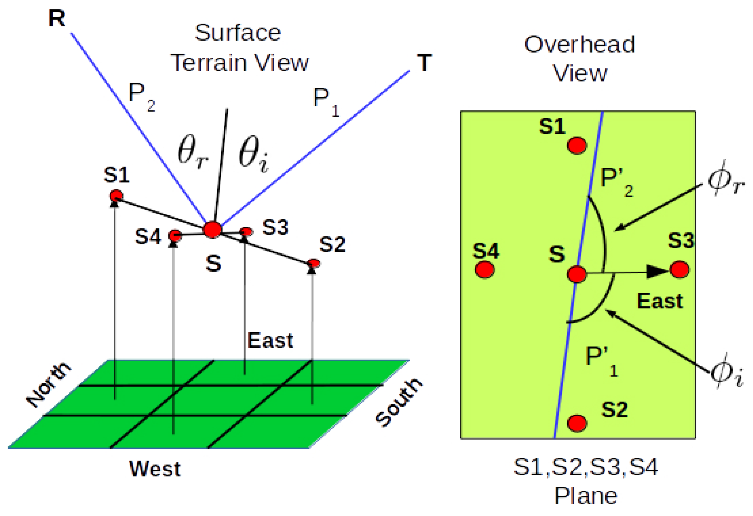
The final check on the land surface geo-location is purely geometrical and is not linked to the signal peak in the received GNSS-R DDM. This check is often the most robust as it is sometimes the case that the CYGNSS-observed delay and Doppler values can be difficult to estimate with certainty due to low receiver antenna gain or adverse Earth surface properties. a reference frame to facilitate the calculation of the incidence and scattering angles from a local surface was defined and is illustrated in Figure 1. With respect to this figure, the following points are defined: S is the center pixel in a 3 by 3 group on the local surface grid, and S1, S2, S3 and S4 are points at pixels directly to the north, south, east and west, respectively, spaced typically at 1 km. The points T and R are the GNSS transmitter and instrument receiver satellite, respectively, while and are the line-of-sight paths from the transmitter to a given surface point and from the surface point to the receiver respectively. The , , , and angles represent the incidence and scattering polar and azimuthal angles, respectively, and are the variables to be calculated at every local surface point ( ).
In the example in Figure 1, all 9 points are shown above the WGS84 reference ellipsoid (shown in green). From the 5 local reference points, incidence and scattering angles can be calculated based on the incoming line-of-sight rays to the center pixel from the transmitter and receiver. We define local east, north, up (ENU) unit vectors from the center reference pixel, S, as follows:
Subsequently, the projected line-of-sight ray paths from the transmitter to the center surface pixel from the center pixel to the receiver ( and , respectively, in Figure 1) are projected to the local surface ENU surface reference frame directions:
From these unit vectors it is possible to calculate the polar and azimuth angles shown in Figure 1 as
We are interested in the difference between the calculated angles and an ideal forward specular reflection from the given surface point. The resulting angle differences from a specular reflecting geometry are then
We define the total angular error metric as the sum of the absolute errors in the azimuth and elevation angles relative to that of an ideal specular reflection,
2.4. Summary of Geolocation Estimation Criteria
The three geolocation parameter checks described above are computed over the local surface grid around the initial estimate of the specular reflection point. If each criteria check is within limits for a given grid point, it is likely that this location is contributing to the received GNSS-R observation. The limits are determined by the geolocation requirements for a given application. Table 1 summarizes the three criteria and the limits used during the analysis that follows.
The limits in Table 1 were selected to achieve an approximate geolocation accuracy of 1 km or less (although results will vary depending on the amplitude of the terrain variations). The algorithm also assigns a confidence level to each geolocation, as specified in Table 2 based on whether any points can be identified within the local surface grid that satisfy the three conditions and based on the DDM SNR.
2.5. Land Geolocation Example
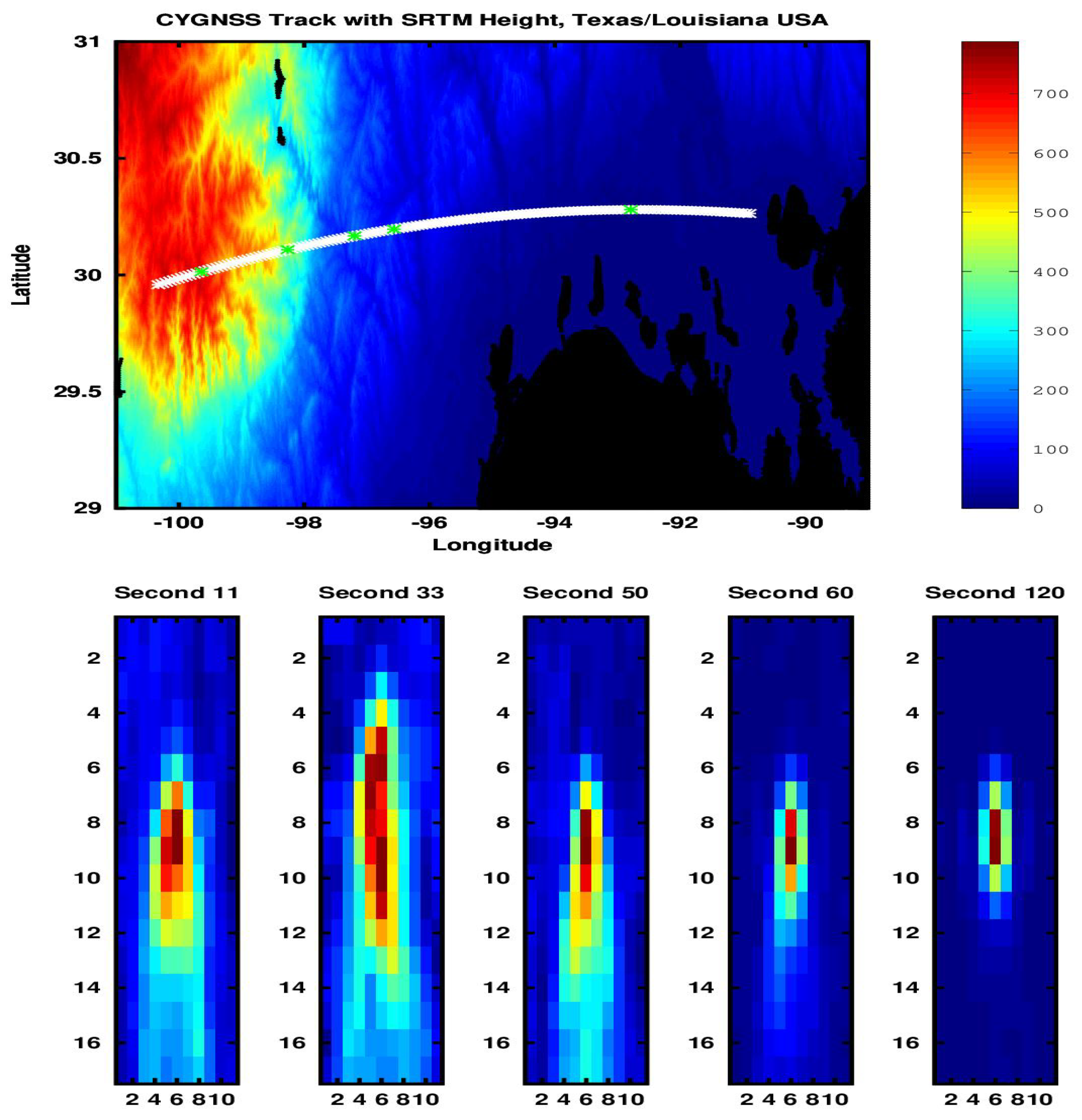
An example land surface reflection track is shown in Figure 2. The track starts in South Texas (the western most point of the track) and extends toward the east to approximately Lake Pontchartrain in Louisiana. Five example observation locations are shown along the track from west to east at relative seconds; 11, 33, 50, 60 and 120, respectively, indicated as consecutive green markers. The corresponding 5 DDMs at these seconds are shown below the track map. These DDMs start as predominantly non-coherent reflections to the west at higher altitude and more varied topography and proceed down in altitude toward sea level and a region with a significant surface water and wetlands coverage. The geolocation results of each of the 5 example DDMs can be briefly summarized as follows:
- Second 11: Relatively high terrain with a varied surface topography. The reflected power appears incoherent, with high confidence in the geolocation.
- Second 33: a “double peaked” DDM, which complicates geolocation determination. Delay and Doppler location checks are based on the highest of the DDM power peaks, which in this case is ambiguous. This “double peak” DDM (with one peak at delay bin 6, and another at delay bin 10) is due to the irregular topography of the surface reflection at second 33, where two distinct and spatially separated surface locations are meeting the geometric conditions suitable for directing power toward the receiver. Attempts at surface retrievals using this DDM would be problematic.
- Seconds 50 and 60: Surface reflections transition from rougher more varied topography to the flatter terrain of western Louisiana. The corresponding DDMs transition from noncoherent at second 50 to largely coherent at second 60.
- Second 120: An area containing multiple surface water bodies within and near the estimated geolocation region. The DDM itself shows a very strong coherent reflection within a limited region around the estimated specular point.
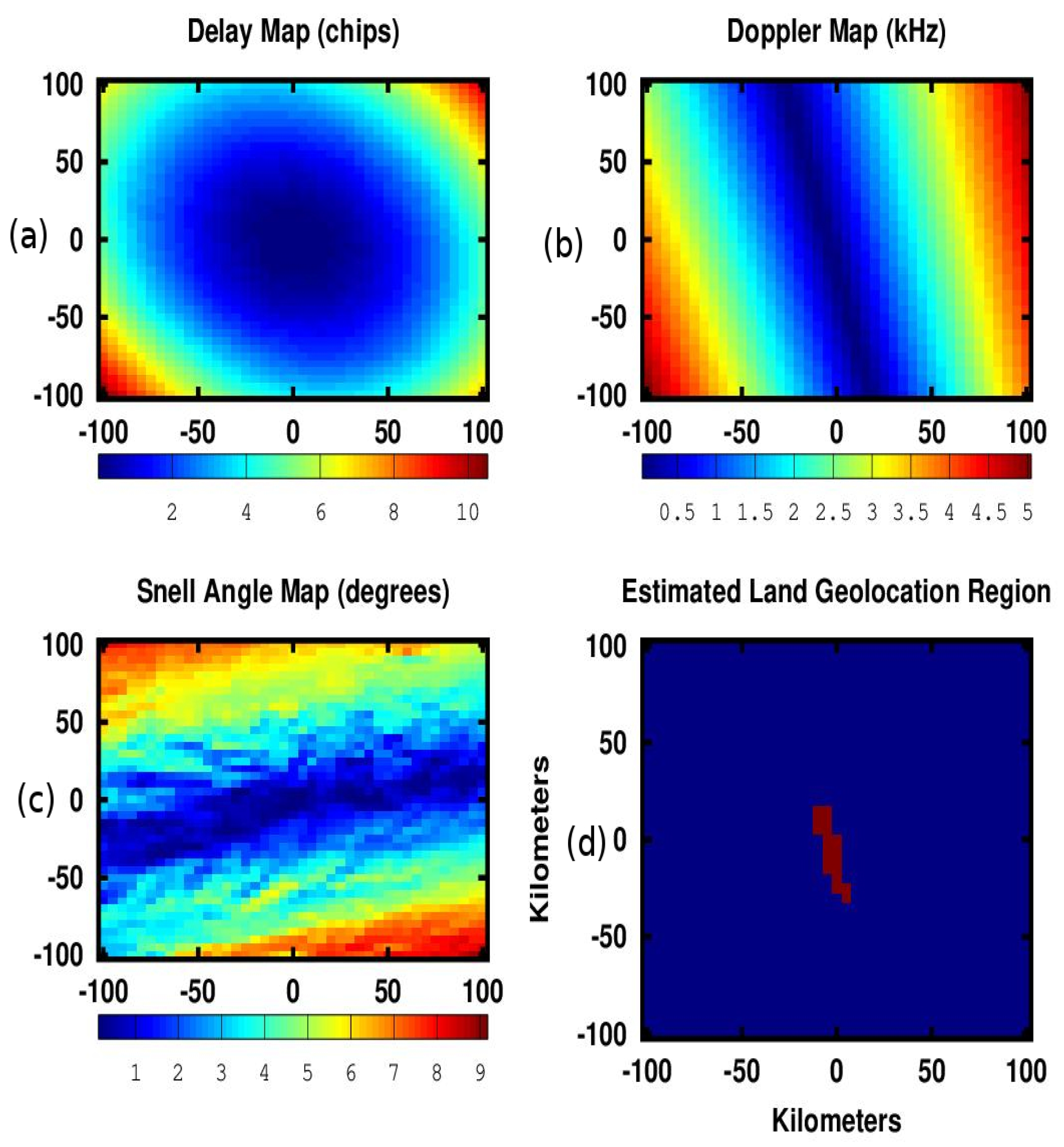
The local surface contour maps used in the geolocation at Second 11 are shown in Figure 3. The top-left plot shows how the delay difference of the Second 11 DDM (peak roughly in bin 8 in Figure 2 (bottom-left)) maps across the 205 km × 205 km local surface grid. The dark area around the initial prediction center clearly indicates that the surface region that corresponds to the peak delay is near the estimated center. The Doppler difference map shown on the top-right further narrows the surface region of interest. Finally, the reflection geometry difference angle (bottom-left) isolates the likely scattering region. These three criteria combined result in the estimated surface geolocation region shown in the bottom-right, where the estimated geolocation for this DDM is predicted to extend over several 1 km surface pixels at and around the center of the local area grid. This geolocation estimate provides the center location of a larger diffuse scattering region (10 km or more).
These local surface maps are calculated for each estimated land reflection point using a global (1 km resolution) SRTM surface height map, cropped around the initial geolocation estimate. This adds considerably to the processing overhead for geolocating each measurement, but is necessary to provide confidence in the predicted surface location of the received signal power, especially as the terrain becomes more varied. In some extreme cases (i.e., mountain regions), the local area maps often reveal highly irregular and discontinuous surface regions which are not always in agreement between each of the three confidence checks. In these cases the geolocation is classified as low confidence and a detailed individual DDM analysis would be required to recover the observations at these locations.
For the DDMs showing coherent reflection (such as seconds 60 and 120), the received power is received from a small area (approx. 1 km) near the predicted geolocation center pixel. The actual surface resolution in the case of coherent reflections is investigated further in Section 4.
2.6. Global Assessment of Land Geolocation Confidence
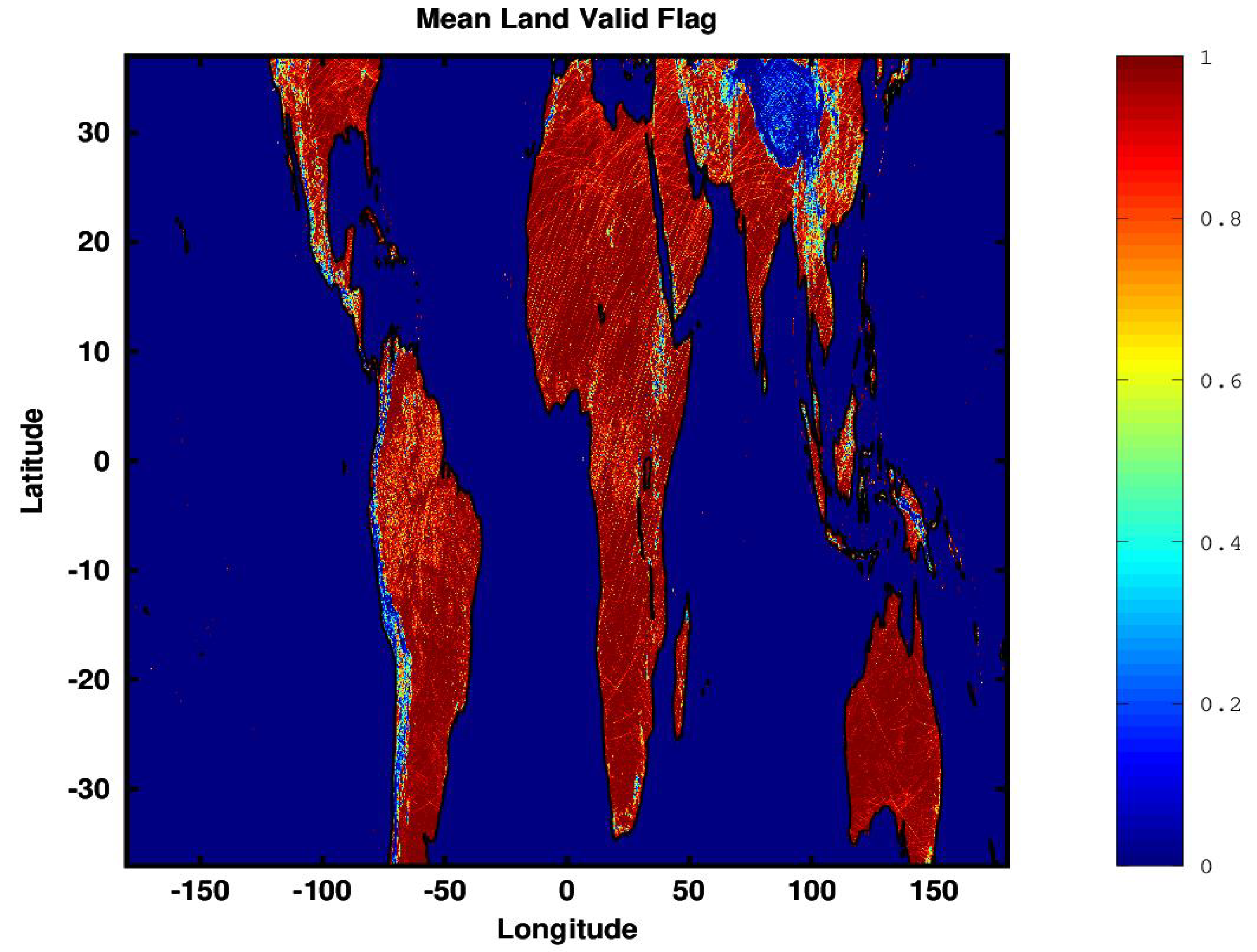
GNSS-R observation geometries for which at least one local grid point satisfying the delay, Doppler and Snell criteria is located are defined as valid geolocation while other cases are classified as invalid geolocation. Figure 4 is a map resolved into 0.1 by 0.1 degree pixels of the fraction of valid geolocations using 12 days of data from all 8 CYGNSS observatories. Note that mean validity values between zero and one are possible due to the multiple looks within a map pixel from varying CYGNSS look angles.
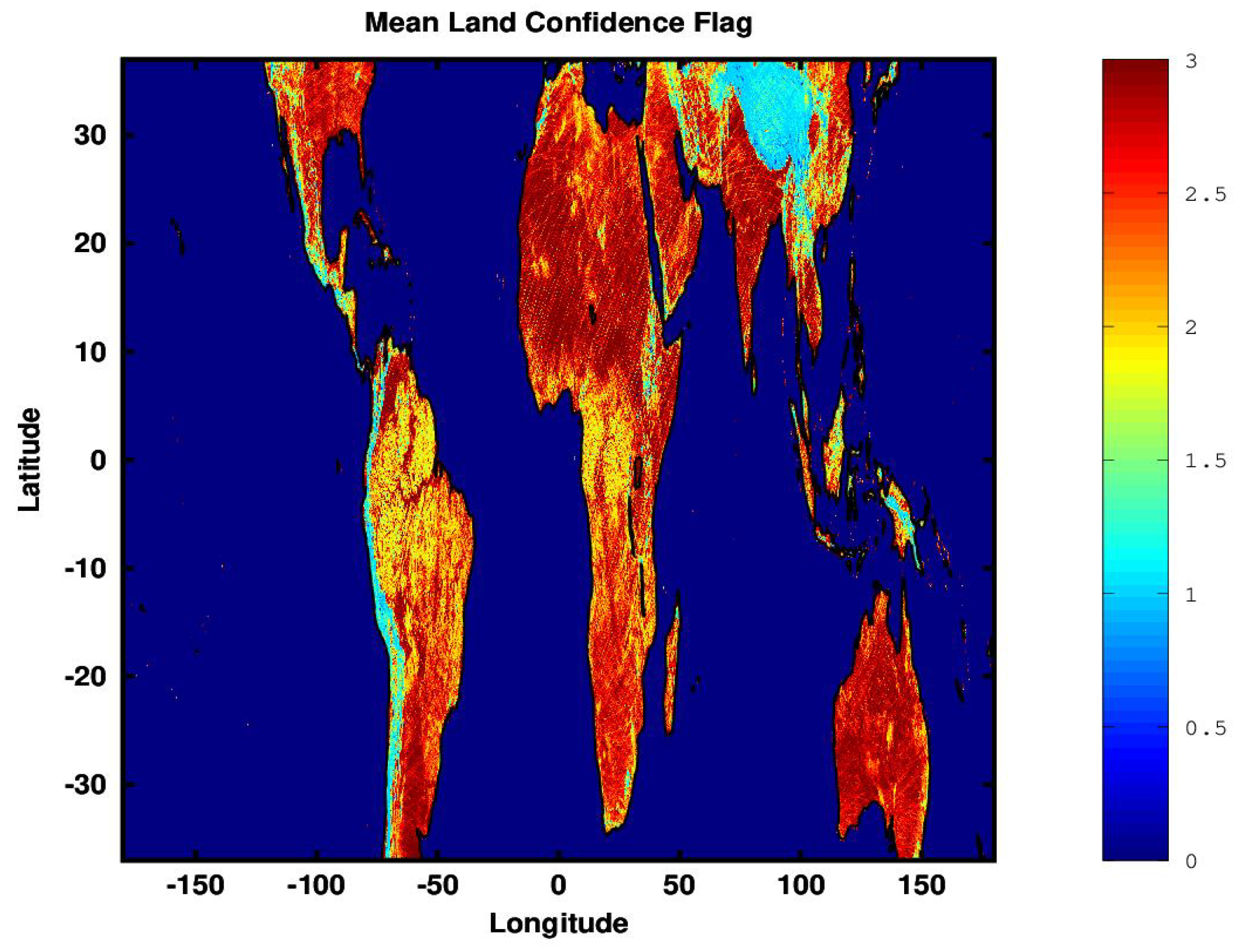
The geolocation confidence flag (which includes the effects of DDM SNR as defined in Table 2) is shown in Figure 5. The results show the frequent high confidence values in most regions excepting those areas having high topographic variations. The percentage of the Earth’s land surface in each confidence category are also included in Table 2). The global Earth land coverage percentage of observations estimated to be valid (confidence level greater than 2) was found to be 77.2%.
3. Calibration of GNSS-R Land Reflections
The conversion of CYGNSS-observed count values into calibrated bistatic radar cross section (BRCS) or surface reflectivity information also requires reconsideration for land surfaces.
3.1. Level 1 Normalized Bistatic Radar Cross Section (NBRCS) Land Calibration
The Level 1a conversion from instrument counts to received power (P in Watts) is performed using the same formulation as for the CYGNSS ocean L1a calibration [9]:
where C and are the total Level 0 counts and noise counts, and are the black body calibration load counts and external noise power, respectively, and is the instrument noise power. All of these parameters are calculated exactly as in the ocean L1a calibration with the exception of the DDM noise counts . The value of is obtained from portions of the DDM that occur at times prior to the specular reflection point, so that only thermal noise is present. Because the delay and Doppler location of ocean DDM returns can be reliably predicted using the WGS84 ellipsoid, a fixed set of time offsets from the WGS84 delay is used for computing for ocean observations. Over land, high surface elevations above the WGS84 ellipsoid can cause surface scattering to impinge upon the standard noise time offsets. Therefore, the delays used for computing over land surfaces exclude any points that approach the land surface delay, calculated as
where is the DEM height above the WGS84 ellipsoid specular point, is the WGS84 specular point incidence angle, and is the delay pixel at the ocean surface, or roughly the WGS84 ellipsoid. Whereas for ocean observations is calculated using noise pixels at delays prior to , for land observations is computed using only delays less than . Due to the repeating nature of the GNSS code delay sequences, code phase roll-overs should be corrected accordingly.
The Level 1b conversion from power in Watts (P) to an estimate of the BRCS can be calculated using the same algorithm as for an ocean reflected signal, using the estimated transmitter power and antenna gain, receiver antenna gain and propagation path losses associated with the reflection geometry determined by the land geolocation point [9]):
where is the effective isotropic radiated power (EIRP), including the transmitter power and antenna gain combined, is the receive antenna gain, and are the ranges from the surface to the receiver and transmitter, respectively. The constant accounts for the diffuse scattering spreading terms. The Level 1 BRCS is calculated over a range of delay ( ) and Doppler frequency (f) bins. The delay and frequency bins containing the maximum received BRCS are used to evaluate the estimated surface geolocation point.
3.2. Level 1 Reflectivity Calculation
The surface footprint returning power to the receiver is significantly altered in the case of coherent reflection, as explored in Section 4. In these conditions the surface is most appropriately described using the surface reflectivity rather than BRCS, where reflectivity () is the standard definition used in remote sensing [20]. Under these conditions, the reflection process is modeled using the Friis transmission equation:
The key difference with the diffuse bistatic equation [11]) is the scaling by the total path length squared as opposed to the squares of the separate transmit and receive path lengths, as the signal reflects and does not diffusely scatter at the surface. The above equation can be rearranged into an expression of surface reflectivity as
where is the level 1a DDM of received power in Watts. Considering the smaller reflection area, it is often useful to consider only the maximum power pixel in the DDM, representing the power level received within a small area near the estimated geolocation point, such that,
3.3. Distinguishing Coherent and Incoherent Returns
It is widely known from surface reflection and scattering theory that the surface properties determine the physical mechanism of electromagnetic radiance scattered from the surface toward the instrument [11,20]. Generally, if the surface is smooth with respect to the incident radiation (in this case the GPS L1 C/A code signal, at approximately 19 cm wavelength) the result will be a coherent reflection. Conversely, relatively rough surfaces with respect to the EM wavelength will result in diffuse scattering toward the instrument. Each of these cases result in distinctly different equations to estimate the surface parameter of interest: for coherent reflection the surface reflectivity, for diffuse scattering the NBRCS.
Considering this duality of possible physical reflection/scattering mechanisms, for land GNSS-R observations it is advisable to calculate both the NBRCS and the surface reflectivity for every CYGNSS DDM. To assist the user in determining which is most appropriate for a given DDM, a flag for identifying the presence of coherence was developed. This flag is based on assessment of the degree of “power spreading” in a DDM, and is described in detail in [13]. It is acknowledged that this flag retains some uncertainty, motivating the reporting of both the NBRCS and reflectivity for all land observations.
3.4. Level 1 Land Calibration Results
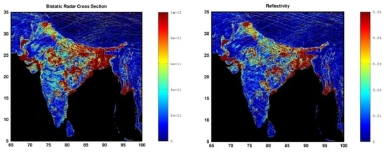
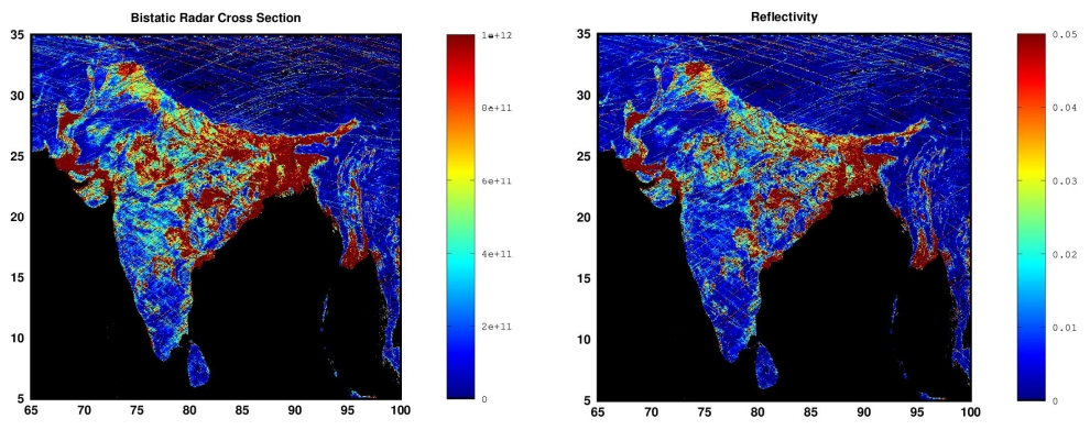
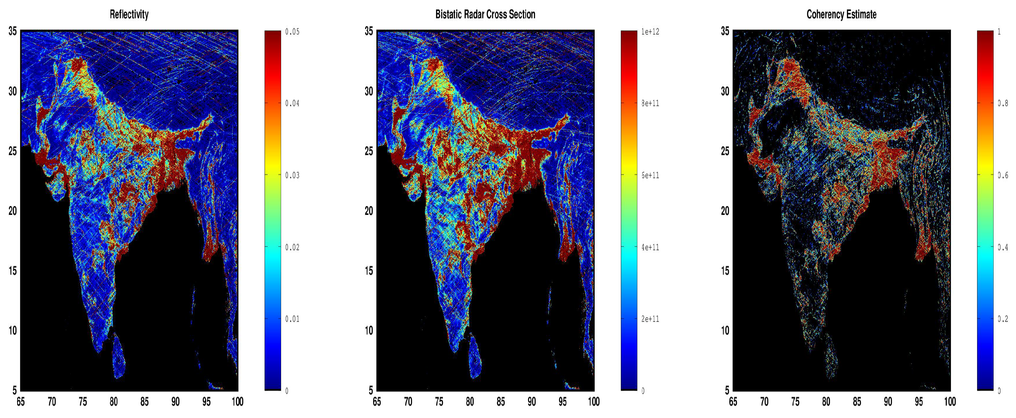
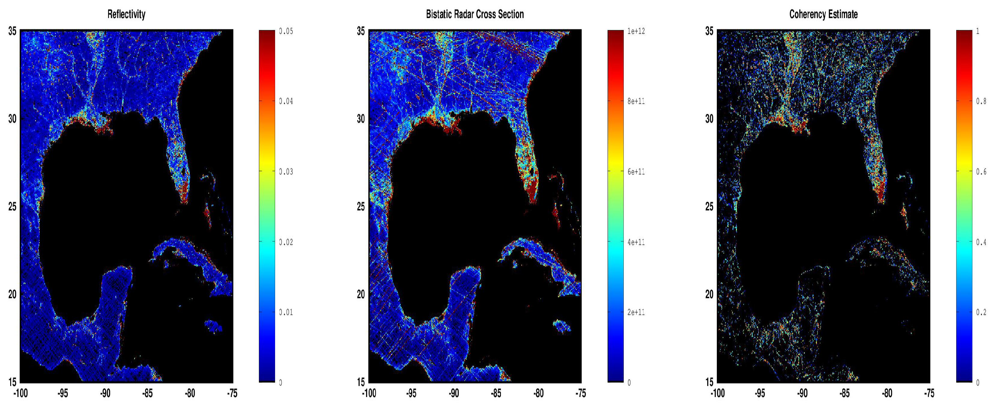
The specified land calibration algorithms were tested using 12 days of CYGNSS data. Two regions were analyzed at finer resolution to better illustrate the differences in NBRCS and reflectivity over known wetlands and regions of higher likelihood of coherent reflection: the southern U.S. and Gulf of Mexico region and the greater Indian Peninsula. Maps of the mean surface reflectivity, mean NBRCS, and coherence flag are shown in Figure 6. Regions of high coherent reflection correlate well with the regions of high reflectivity and NBRCS and with known regions having a high prevalence of inland water bodies.
4. Analysis of Coherent Surface Resolution Using Ancillary River Width Data
To assess CYGNSS’s spatial resolution under the conditions of coherent reflection quantitatively, we have performed a statistical study using the North American River Width Data Set (NARWidth) [21]. This dataset provides a reference for locations with greater expectation of generating a coherent reflection. The RMS error of the NARWidth river data set, compared to in-situ measured river widths, is estimated to be approximately 38 m [21]. a detailed coherency analysis using raw sampled data from CYGNSS (from which coherent phase information can be estimated) was previously presented in [22]. However, this work presents CYGNSS results in its normal processing mode (including the non-coherent instrument integration which eliminates all phase information in the observable).
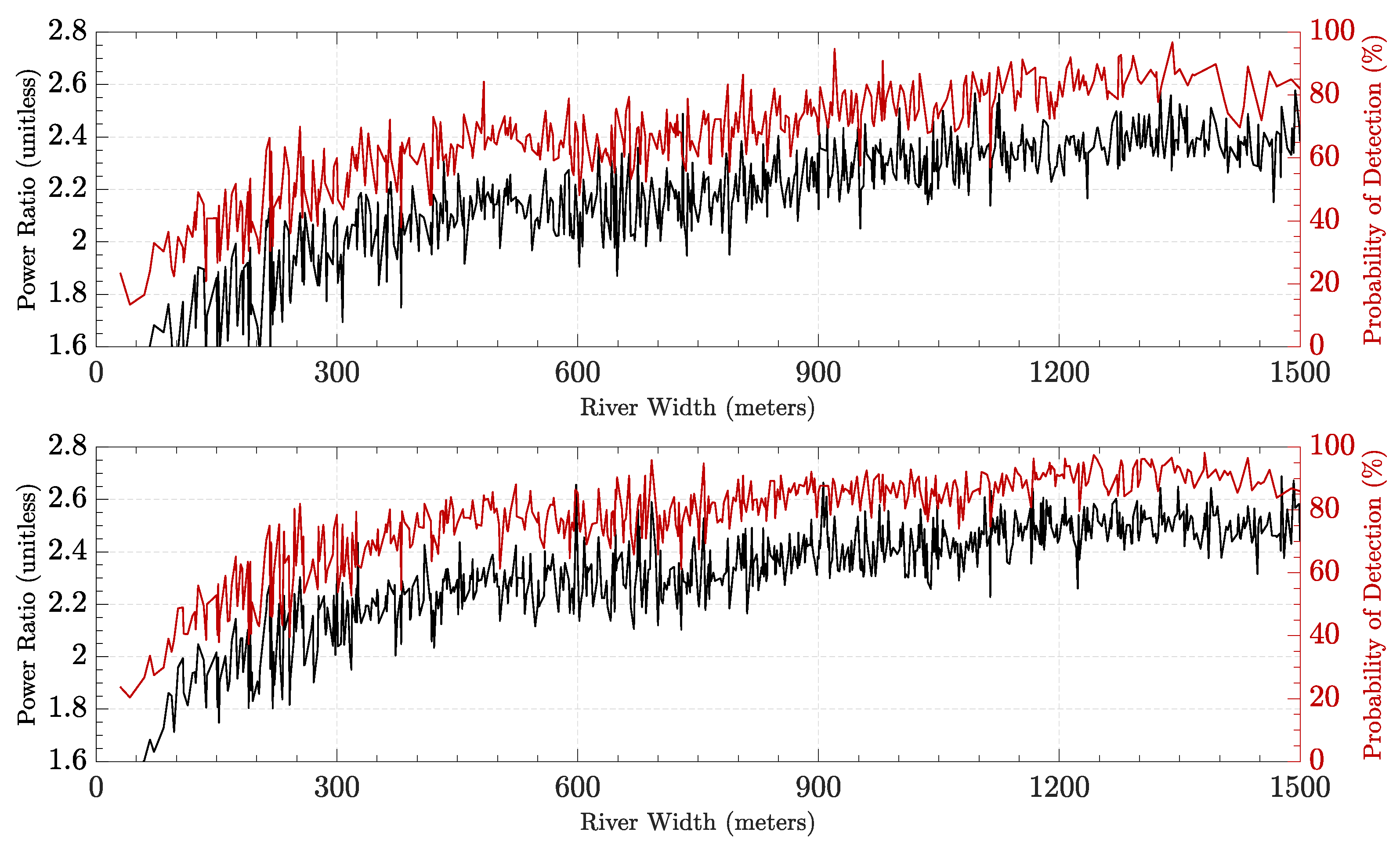
Using the available CYGNSS measurements together with reported river widths, the mean Level-1 power ratio coherence metric with respect to varying river widths is examined in Figure 7. The is an estimate of the ratio of the amount of received power near the peak to the integrated power away from the peak, derived in [13]. Increasing river widths were found to be associated with a steady increase in the Level-1 coherence metric and the probability of detecting the river, with the detection probability approaching 100% for rivers with widths exceeding ≈ 1.2 km. This is to be expected as rivers with larger widths present a target more conducive to result in identifiable coherence characterized by a significant concentration of power about the DDM peak. They are also less susceptible to ambiguities introduced by the L1 integration time(s) as well as perturbations associated with more heterogeneous scenes. It is also noted that operationally, a DDM measurement is declared as being the result of a dominantly coherent reflection process if its power ratio exceeds the detection threshold = 2.0.
From the analysis presented in Figure 7 it is observed that this occurs, on average, for rivers with a minimum width exceeding 250 m and 200 m for 1 Hz and 2 Hz CYGNSS data, respectively. This places a minimum bound on the finest spatial features CYGNSS measurements are able to resolve, on average, suggesting that this is on the order of a first Fresnel zone and provides empirical support for previous theoretical treatments of this question [23]. However, there are several caveats to this analysis which assumes that rivers will generally satisfy the conditions to produce coherent CYGNSS forward reflections:
- River widths are known to change dynamically, seasonally and during flooding events. The NARWidth data set provides an estimate of the river width at mean discharge, thus it does not account for natural seasonal variations. The analysis undertaken here focuses on using CYGNSS data over two eight month periods, the first starting with July 2018 and ending with February 2019 and the second starting with July 2019 and ending with February 2020. This included a total of 50 million measured CYGNSS specular points, within the NARWidth dataset’s coverage, providing ample data to generate statistically significant results. While variations in the size of the coherent reflection surface due to natural fluctuations in river widths will contribute errors into the analysis, the mean correspondence of measures of interest to varying river widths is expected to remain indicative of CYGNSS’s spatial resolution under conditions of coherent reflection.
- Previous analysis of CYGNSS data has shown that river surfaces are generally smooth enough to result in coherent forward reflections [6]. However, there will be cases when a river surface is rough relative to the reflecting L-band wavelength (19 cm) and will not generate coherent forward reflections. In these circumstances, the area of surface scattering will be significantly larger than an integrated Fresnel zone and not result in coherent detection of the river crossing.
- After (approximately) July 2019, the CYGNSS output data rate was increased from 1 Hz to 2 Hz Level 0 observations. The 2 Hz data output rate corresponds to a 0.5 s instrument integration interval, which reduces the length that the single look surface footprint is integrated across the surface at the specular point velocity. Generally, CYGNSS 1 Hz observations result in a surface integration on the order of 6 km in the along track direction due to satellite motion, while 2 Hz observations will span roughly half of that distance. Note that short intervals of coherent reflection (such as from a small water bodies) within the larger integration footprint often dominate the received power, resulting in detections of small water bodies within the longer integrated surface footprint.
- Horizontal errors in the surface geolocation of reflections near the Courantyne river will potentially introduce small errors (less than ≈ 1 km) in the river width estimates.
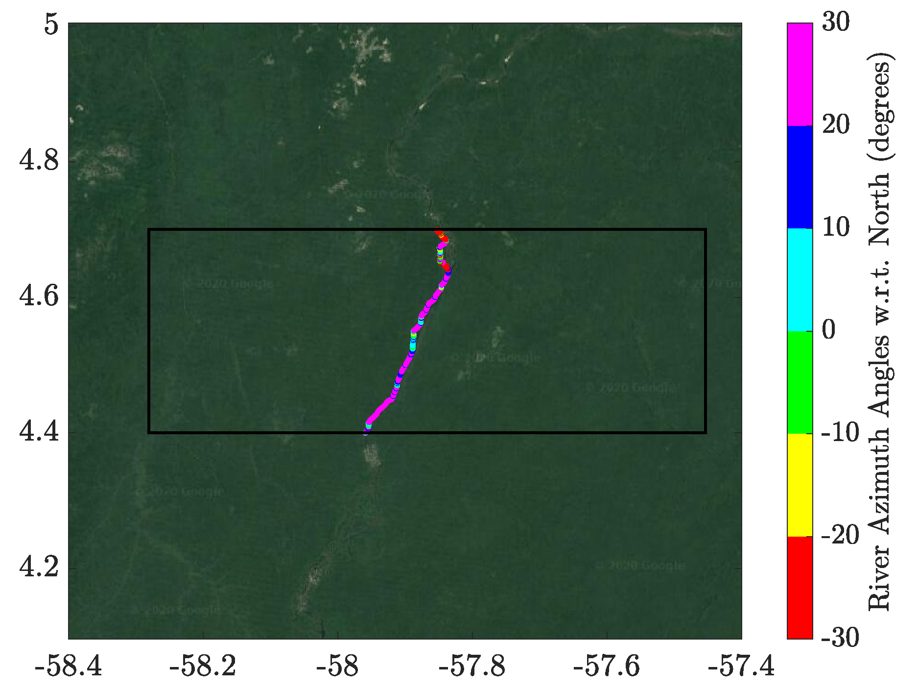
The upper bound of the constellation’s ability to resolve features on the surface, under a coherent reflection regime, is expected to be governed by the incoherent integration time. The reduction of the integration interval reduces the along track smearing of L1 DDMs, thereby improving the overall spatial resolution. To illustrate this, CYGNSS measurements from over a (mean) 500 m wide section of the Courantyne River were analyzed, illustrated in Figure 8, over 8 month periods when the constellation operated exclusively in 1 Hz and 2 Hz modes. Details of the selected test region and CYGNSS track crossings are described in Table 3.
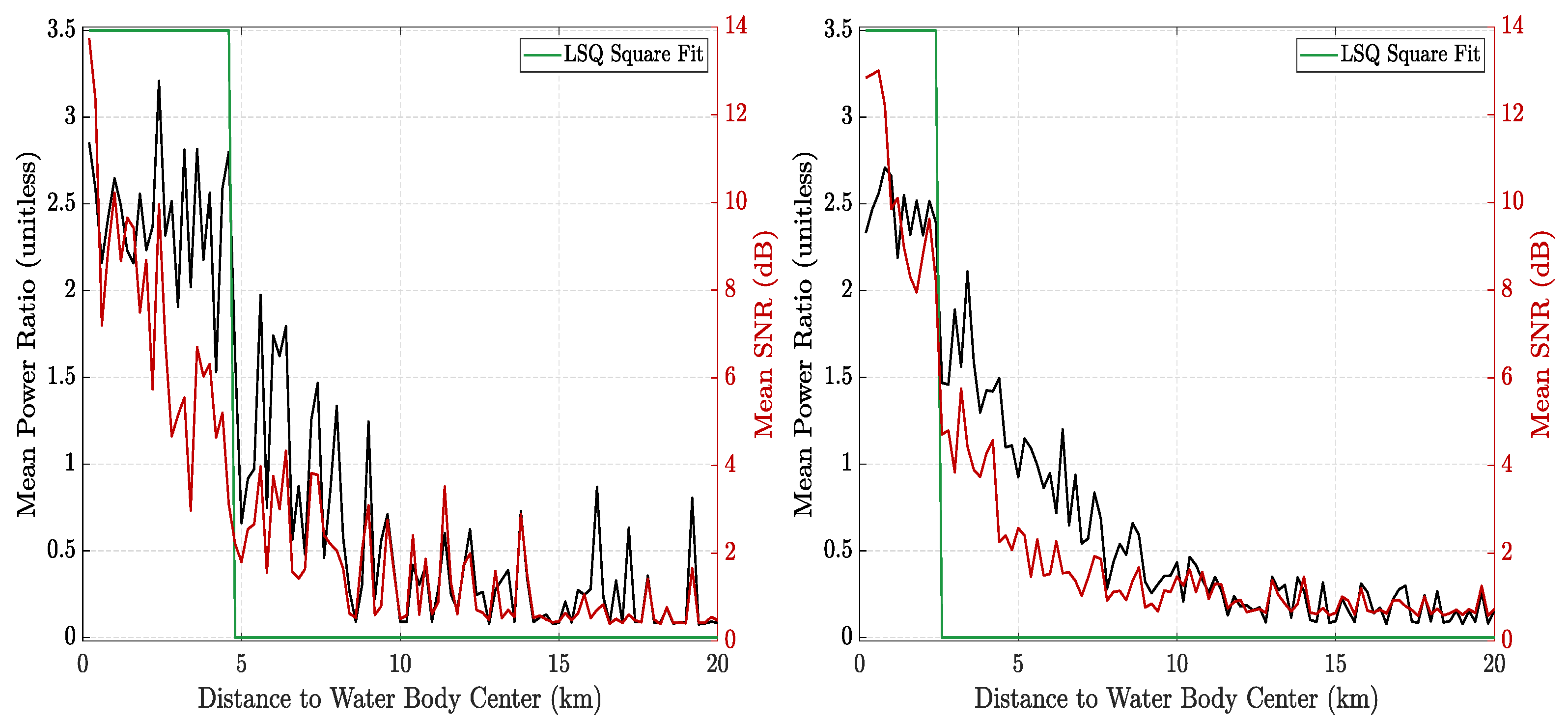
As illustrated in Figure 9, it can be observed that the 1 Hz CYGNSS data mean power ratios remain above the detection threshold for distances up to 5 km, slightly less than the ≈6 km distances traveled during the 1 s integration time. Within this 5 km radius, the is maintained above the detection threshold as the result of dominant coherent reflections arising from the (mean) 500 m wide river. The contributions of the coherent reflector (the river) get ‘smeared’ along track thereby degrading the surface resolution of the individual observation. This is contrasted with the behavior of measurements made after the switch to 2 Hz sampling over the same region where it is observed that due to the halving of the incoherent integration time, the along track smearing is reduced to approximately the distance traveled along track between two consecutive specular points of ≈3 km. As a result, the power ratios are estimated as ‘dominantly coherent’ up to 2.4 km away from the river center resulting in an average improvement in spatial resolution of ≈48% brought about by the reduction in integration time. a summary of the observation statistics based on the data shown in Figure 9, is included in Table 4.
5. Discussion
This manuscript addresses several of the underlying requirements unique in the processing of GNSS-R land observations: geolocating the observations in diverse topography, calibration the observations into both reflectivity and NBRCS estimates, and assessing the surface resolution for the coherent reflection case.
We have shown that in a majority of CYGNSS land observations we were able to predict the surface observation point with high confidence. This can generally be attributed to many regions of the Earth having relatively low and moderate surface topographic variations, and those variations often being more or less consistent over kilometer scales. However, the exceptional cases in extreme environments will often be incompatible with a generalized algorithm and will require detailed per-DDM analysis across larger regions to identify the locations generating the received power at the instrument.
As discussed above, the increased likelihood of complexities associated with the presence of coherent (and mixed) observations as well as diffuse scattering from land surfaces, can be mitigated with a dual approach for land observations that estimates both surface reflectivity and NBRCS, accompanied by an additional estimate as to the coherence in the level 0 observation. This approach assumes that individual users working on higher level geophysical parameter estimation will need to consider carefully how they apply the different surface observations in conjunction with the provided (or independently estimated) likelihood of signal coherency.
We feel this initial study on the detectable surface resolution of small coherent surface features provides a useful first quantitative analysis of the impact of the non-coherent instrument integration and the resulting blurring of surface footprint and how this impacts the detection of small features within a larger integrated surface area. The surface resolution in the case of diffusely scattered land observations is a subject of further study and expected to be more on the order of the surface resolution of a typical ocean observation (on the order of 15 km or greater).
6. Results
This paper presents an algorithm for the geolocation of CYGNSS observations over diverse terrain conditions. Three criteria were used in the assessment of surface regions for the likelihood of directing power toward the GNSS-R receiver: delay iso-surface range agreement, Doppler iso-surface frequency agreement, and forward reflection Snell angle geometry. It was found that it was possible to estimate the geo-location point of the land reflected signal accurately (mean confidence level of greater than 2) over more than 77.2% of the Earth’s land surface. It was also observed that in more complicated terrain environments it is possible for multiple surface areas to contribute to a single GNSS-R observation, thus making observation geolocation inherently problematic.
Additionally, a dual approach level 1 land calibration algorithm was presented which calculates both the BRCS and the surface reflectivity for every land DDM. It was proposed that the CYGNSS level 1 DDM coherency estimator could be used to assist in the determination of the physical scattering or reflection conditions and guide which surface parameter to apply (reflectivity or NBRCS) during land geophysical parameter retrievals. Reflectivity and BRCS maps over regions of varied coherent reflection were presented using 12 days of data from the NASA CYGNSS mission.
Finally, an investigation was performed to quantify the the CYGNSS surface resolution for coherently reflected land signals, and to assess the probability of small water body detection, using the NARWidth Data Set of mean river widths. The resulting analysis showed that (for a 500 m mean width river), the CYGNSS level-1 coherence detector could be used to estimate the bounds of the surface detection resolution with respect to the incoherent integration interval. The resulting detection resolution was determined to be 4600 m for 1 Hz observations (1 s intergation) and 2400 m for 2 Hz observations (0.5 s integration). This clearly demonstrates the advantage (48% improvement) with the shorter integration intervals in the detection of land coherent water bodies.
Author Contributions
S.G.: methodology, validation, writing, review and editing, all Sections. A.O.: methodology, Section 2. A.R.: software, Section 2 and Section 3. M.M.A.-K.: methodology and formal analysis, Section 4. J.T.J.: methodology and supervision, all Sections. All authors have read and agreed to the published version of the manuscript.
Funding
This research was funded by the NASA Earth Ventures Cyclone Global Navigation Satellite System (CYGNSS), Extended Mission.
Conflicts of Interest
The authors declare no conflict of interest.
Abbreviations
The following abbreviations are used in this manuscript:
| CYGNSS | Cyclone Global Navigation Satellite System |
| GNSS | Global Navigation Satellite System |
| GPS | Global Positioning System |
| GNSS-R | Global Navigation Satellite System Reflectometry |
| DDM | Delay Doppler Map |
| PR | Power Ratio |
| BRCS | Bistatic Radar Cross Section |
| NBRCS | Normalized Bistatic Radar Cross Section |
| NARWidth | North American River Width Data Set |
| DEM | Digital Elevation Model |
| ENU | East, North, Up |
| SNR | Signal to Noise Ratio |
| SRTM | Shuttle Radar Topography Mission |
| WGS84 | World Geodetic System 1984 |
References
- Misra, P.; Enge, P. Global Positioning System: Signals, Measurements, and Performance; Ganga Jamuna Press: Lincoln, MA, USA, 2001; ISBN 0-9709544-0-9. [Google Scholar]
- Gebre-Egziabher, D.; Gleason, S. GNSS Applications and Methods; Artech House: Norwood, MA, USA, 2009. [Google Scholar]
- Gleason, S. Remote Sensing of Ocean, Ice and Land Surfaces Using Bistatically Scattered GNSS Signals From Low Earth Orbit. Ph.D. Thesis, University of Surrey, Guildford, UK, 2006. [Google Scholar]
- Masters, D.; Katzberg, S.; Axelrad, P. Airborne GPS bistatic radar soil moisture measurements during SMEX02. In Proceedings of the 2003 IEEE International Geoscience and Remote Sensing Symposium (IGARSS 2003), Toulouse, France, 21–25 July 2003; Volume 2, pp. 896–898. [Google Scholar]
- Ruf, C.S.; Asharaf, S.; Balasubramaniam, R.; Gleason, S.; Lang, T.; McKague, D.; Twigg, D.; Waliser, D. In-Orbit Performance of the Constellation of CYGNSS Hurricane Satellites. Bull. Am. Meteorol. Soc. 2019, 100, 2009–2023. [Google Scholar] [CrossRef]
- Chew, C.; Reager, J.T.; Small, E. CYGNSS data map food inundation during the 2017 Atlantic hurricane season. Sci. Rep. 2018, 8, 9336. [Google Scholar] [CrossRef] [PubMed]
- Chew, C.C.; Small, E.E. Soil Moisture Sensing Using Spaceborne GNSS Reflections: Comparison of CYGNSS Reflectivity to SMAP Soil Moisture. Geophys. Res. Lett. 2018, 45, 4049–4057. [Google Scholar] [CrossRef] [Green Version]
- Al-Khaldi, M.M.; Johnson, J.T.; O’Brien, A.J.; Balenzano, A.; Mattia, F. Time-Series Retrieval of Soil Moisture Using CYGNSS. IEEE Trans. Geosci. Remote. Sens. 2019, 57, 4322–4331. [Google Scholar] [CrossRef]
- Gleason, S.; Ruf, C.S.; Clarizia, M.P.; O’Brien, A.J. Calibration and Unwrapping of the Normalized Scattering Cross Section for the Cyclone Global Navigation Satellite System. IEEE Trans. Geosci. Remote. Sens. 2016, 54, 2495–2509. [Google Scholar] [CrossRef]
- Gleason, S. CYGNSS Algorithm Theoretical Basis Documents, Level 1A and 1B; University of Michigan: Ann Arbor, MI, USA, 2018. [Google Scholar]
- Zavorotny, V.; Voronovich, A. Scattering of GPS signals from the ocean with wind remote sensing application. IEEE Trans. Geosci. Remote. Sens. 2000, 38, 951–964. [Google Scholar] [CrossRef] [Green Version]
- Yardim, C.; Johnson, J.T.; Burkholder, R.; Teixeira, F.L.; Ouellette, J.D.; Chen, K.-S.; Brogioni, M.; Pierdicca, N. An intercomparison of models for predicting bistatic scattering from rough surfaces. In Proceedings of the 2015 IEEE International Geoscience and Remote Sensing Symposium (IGARSS), Milan, Italy, 26–31 July 2015; pp. 2759–2762. [Google Scholar] [CrossRef]
- Al-Khaldi, M.M.; Johnson, J.T.; Gleason, S.; Loria, E.; Yi, Y. An Algorithm for Detecting Coherence in Cyclone Global Navigation Satellite System Mission Level 1 Delay Doppler Maps. IEEE Trans. Geosci. Remote Sens. 2019. under review. [Google Scholar]
- Carreno-Luengo, H.; Luzi, G.; Crosetto, M. First Evaluation of Topography on GNSS-R: An Empirical Study Based on a Digital Elevation Model. Remote. Sens. 2019, 11, 2556. [Google Scholar] [CrossRef] [Green Version]
- Camps, A.; Park, H.; Pablos, M.; Foti, G.; Gommenginger, C.; Liu, P.-W.; Judge, J. Sensitivity of GNSS-R Spaceborne Observations to Soil Moisture and Vegetation. IEEE J. Sel. Top. Appl. Earth Obs. Remote. Sens. 2016, 9, 4730–4742. [Google Scholar] [CrossRef] [Green Version]
- Comite, D.; Ticconi, F.; Dente, L.; Guerriero, L.; Pierdicca, N. Bistatic Coherent Scattering From Rough Soils with Application to GNSS Reflectometry. IEEE Trans. Geosci. Remote. Sens. 2020, 58, 612–625. [Google Scholar] [CrossRef]
- Gleason, S. A Real-Time On-Orbit Signal Tracking Algorithm for GNSS Surface Observations. Remote. Sens. 2019, 11, 1858. [Google Scholar] [CrossRef] [Green Version]
- Gleason, S.; Ruf, C.S.; O’Brien, A.J.; McKague, D.S.; OrBrien, A.J. The CYGNSS Level 1 Calibration Algorithm and Error Analysis Based on On-Orbit Measurements. IEEE J. Sel. Top. Appl. Earth Obs. Remote. Sens. 2019, 12, 37–49. [Google Scholar] [CrossRef]
- Shuttle Radar Topography Mission (SRTM). Available online: https://www.usgs.gov/centers/eros/ (accessed on 16 November 2018).
- Ulaby, F.T.; Long, D.G. Microwave Radar and Radiometric Remote Sensing; University Michigan Press: Ann Arbor, MI, USA, 2014. [Google Scholar]
- Allen, G.H.; Pavelsky, T.M. Patterns of river width and surface area revealed by the satellite-derived North American River Width data set. Geophys. Res. Lett. 2015, 42, 395–402. [Google Scholar] [CrossRef]
- Loria, E.; O’Brien, A.; Gupta, I.J. Detection and Separation of Coherent Reflections in GNSS-R Measurements Using CYGNSS Data. In Proceedings of the 2018 IEEE International Geoscience and Remote Sensing Symposium 2018 (IGARSS 2018), Valencia, Spain, 22–27 July 2018; pp. 3995–3998. [Google Scholar] [CrossRef]
- Camps, A. Spatial Resolution in GNSS-R Under Coherent Scattering. IEEE Geosci. Remote. Sens. Lett. 2020, 17, 32–36. [Google Scholar] [CrossRef]
Figure 1.
(left) Surface terrain view of point on local surface grid showing incident and reflection angles with respect to the surface normal. (right) Overhead view with incident and reflected vectors projected to a local two dimensional surface with forward scattering azimuth angles shown.
Figure 1.
(left) Surface terrain view of point on local surface grid showing incident and reflection angles with respect to the surface normal. (right) Overhead view with incident and reflected vectors projected to a local two dimensional surface with forward scattering azimuth angles shown.

Figure 2.
(top) Example Cyclone Global Navigation Satellite System (CYGNSS) reflection track over changing terrain. Image background is Shuttle Radar Topography Mission (SRTM) height map in meters. CYGNSS track shown as white arch traveling from west to east, green stars along track indicate Delay Doppler Map (DDM) locations. Second 11 is the western most green star, Second 120 is the eastern most. Water regions shown in black. (bottom) Example DDMs at points along the track from various terrain conditions.

Figure 3.
Contour maps of the three geolocation checks across local surface grids at second 11 of Figure 2. (a) Empirical delay difference () contour map, (b) Empirical Doppler difference () contour map, (c) Geometric Snell reflection angle difference (), (d) Logical “AND" of the delay, Doppler and Snell area checks, indicating region which satisfies the tolerance limits of all three forward reflection geolocation criteria.

Figure 4.
Map of mean land geolocation validity flag (0 or 1). Areas of lower validity correlate strongly with regions of high terrain variability. CYGNSS is unable to capture DDMS from the Tibetan Plateau and Andes Mountain regions.
Figure 4.
Map of mean land geolocation validity flag (0 or 1). Areas of lower validity correlate strongly with regions of high terrain variability. CYGNSS is unable to capture DDMS from the Tibetan Plateau and Andes Mountain regions.

Figure 5.
Map of land geolocation confidence flag. Confidence values range between 0 (lowest) and 3 (highest). As expected the general trend is that the estimated geolocation is of higher confidence over lower lying and more moderate terrain. It can also be observed that the geolocation often more difficult in dense forest regions (South America and Central Africa) due to the relatively lower SNR from these surfaces, which make the empirical signal peak checks more difficult.

Figure 6.
(left) Mean surface reflectivity from 12-days of CYGNSS observations. (middle) Mean surface peak bistatic radar cross section (BRCS) over the same 12-days of CYGNSS observations. (right) Estimated mean reflected signal coherency estimate over same 12-day interval (1 = coherent, 0 = non-coherent) for the Indian Peninsula and the Gulf of Mexico regions.


Figure 7.
Analysis deriving from the NARWidth data set illustrating effects of varied river widths on the CYGNSS Level-1 coherence metric and probability of detection. (Top) Across a sixth month period from 1 September 2018 to 28 February 2019, exclusively comprising 1 Hz data. (Bottom) Across a sixth month period from 1 September 2019 to 2 February2020, exclusively comprising 2 Hz data.

Figure 8.
Test region latitude/longitude used in CYGNSS integration time analysis. Test region was centered around a 35 km long section of the Courantyne River between Guyana and Suriname.
Figure 8.
Test region latitude/longitude used in CYGNSS integration time analysis. Test region was centered around a 35 km long section of the Courantyne River between Guyana and Suriname.

Figure 9.
Effects of varying the CYGNSS mission’s Level-1 product integration time for observations in the vicinity of the Courantyne River on the CYGNSS coherence metric and Signal-to-Noise Ratio (SNR) at varying distances from the water body. (Left) From 3 July 2018 to 28 February 2019, exclusively comprising 1 Hz data. (Right) From 3 July 2019 to 28 February 2020, exclusively comprising 2 Hz data. Green traces indicates Least-Squares estimated transition distance between coherence and non-coherence threshold.


Table 1.
Summary of land Geo-location criteria parameters and thresholds used during performance analysis.
Table 1.
Summary of land Geo-location criteria parameters and thresholds used during performance analysis.
| Criteria | Threshold | Verification |
|---|---|---|
| 2.5 C/A Code Chips | Maximum delay | |
| 200 Hz | Maximum Doppler | |
| 2 Degrees | Reflection geometry |
Table 2.
Summary of land geolocation confidence flag logic.
| SNR Thold (2 dB) | Delay, Doppler, Snell | Confidence | Land Percentage | Comment |
|---|---|---|---|---|
| Above | Invalid | 0 | 1.3 (0 to 1) | Most likely incorrect |
| Below | Invalid | 1 | 21.5 (1 to 2) | Probably incorrect |
| Below | Valid | 2 | 28.4 (2 to 2.5) | Likely correct |
| Above | Valid | 3 | 48.8 (2.5 to 3) | High probability correct |
Table 3.
Description of selected test region for river crossing coherency analysis.
| Courantyne River Region (Guyana/Suriname) | ||
|---|---|---|
| Parameter | Mean Value | Comment |
| River Width | 500 m | NARWidth [21] |
| North Angle | 29 deg | Figure 8 |
| Test Region | Min | Max |
| Latitude | 4.4 | 4.7 |
| Longitude | −58.3 | −57.45 |
| Track Direction | North Angle | River Angle |
| Ascending | 53 deg | 24 deg |
| Descending | 127 deg | 97 deg |
Table 4.
Observation statistics and estimated LSQ fit of coherence detection threshold distances (4600 m at 1 Hz, and 2400 m at 2 Hz) for 1 Hz and 2 Hz DDM frequencies.
Table 4.
Observation statistics and estimated LSQ fit of coherence detection threshold distances (4600 m at 1 Hz, and 2400 m at 2 Hz) for 1 Hz and 2 Hz DDM frequencies.
| Parameter | Distance | Mean | STD |
|---|---|---|---|
| 1 Hz DDM Frequency (Obs. Spacing: 5990m) | |||
| Power Ratio | 500 m | 2.38 | 0.77 |
| Power Ratio | 4600 m | 2.41 | 1.54 |
| SNR | 500 m | 9.75 dB | 5.35 dB |
| SNR | 4600 m | 6.63 dB | 5.23 dB |
| Detection Prob. | 500 m | 91.67 % | N/A |
| Detection Prob. | 4600 m | 77.67 % | N/A |
| 2 Hz DDM Frequency (Obs. Spacing: 3010m) | |||
| Power Ratio | 500 m | 2.43 | 0.87 |
| Power Ratio | 2400 m | 2.46 | 1.13 |
| SNR | 500 m | 12.91 dB | 6.48 dB |
| SNR | 2400 m | 10.05 dB | 5.97 dB |
| Detection Prob. | 500 m | 92.16 % | N/A |
| Detection Prob. | 2400 m | 87.12 % | N/A |
© 2020 by the authors. Licensee MDPI, Basel, Switzerland. This article is an open access article distributed under the terms and conditions of the Creative Commons Attribution (CC BY) license (http://creativecommons.org/licenses/by/4.0/).
Share and Cite
MDPI and ACS Style
Gleason, S.; O’Brien, A.; Russel, A.; Al-Khaldi, M.M.; Johnson, J.T. Geolocation, Calibration and Surface Resolution of CYGNSS GNSS-R Land Observations. Remote Sens. 2020, 12, 1317. https://0-doi-org.brum.beds.ac.uk/10.3390/rs12081317
AMA Style
Gleason S, O’Brien A, Russel A, Al-Khaldi MM, Johnson JT. Geolocation, Calibration and Surface Resolution of CYGNSS GNSS-R Land Observations. Remote Sensing. 2020; 12(8):1317. https://0-doi-org.brum.beds.ac.uk/10.3390/rs12081317
Chicago/Turabian StyleGleason, Scott, Andrew O’Brien, Anthony Russel, Mohammad M. Al-Khaldi, and Joel T. Johnson. 2020. "Geolocation, Calibration and Surface Resolution of CYGNSS GNSS-R Land Observations" Remote Sensing 12, no. 8: 1317. https://0-doi-org.brum.beds.ac.uk/10.3390/rs12081317
Note that from the first issue of 2016, this journal uses article numbers instead of page numbers. See further details here.