The Autonomous Underwater Vehicle Integrated with the Unmanned Surface Vessel Mapping the Southern Ionian Sea. The Winning Technology Solution of the Shell Ocean Discovery XPRIZE

 ,
,  , ,
, ,  ,
,
Abstract
:
1. Introduction
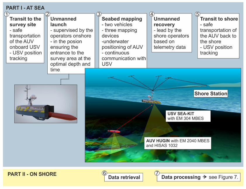
2. Methods
2.1. Data Acquisition System
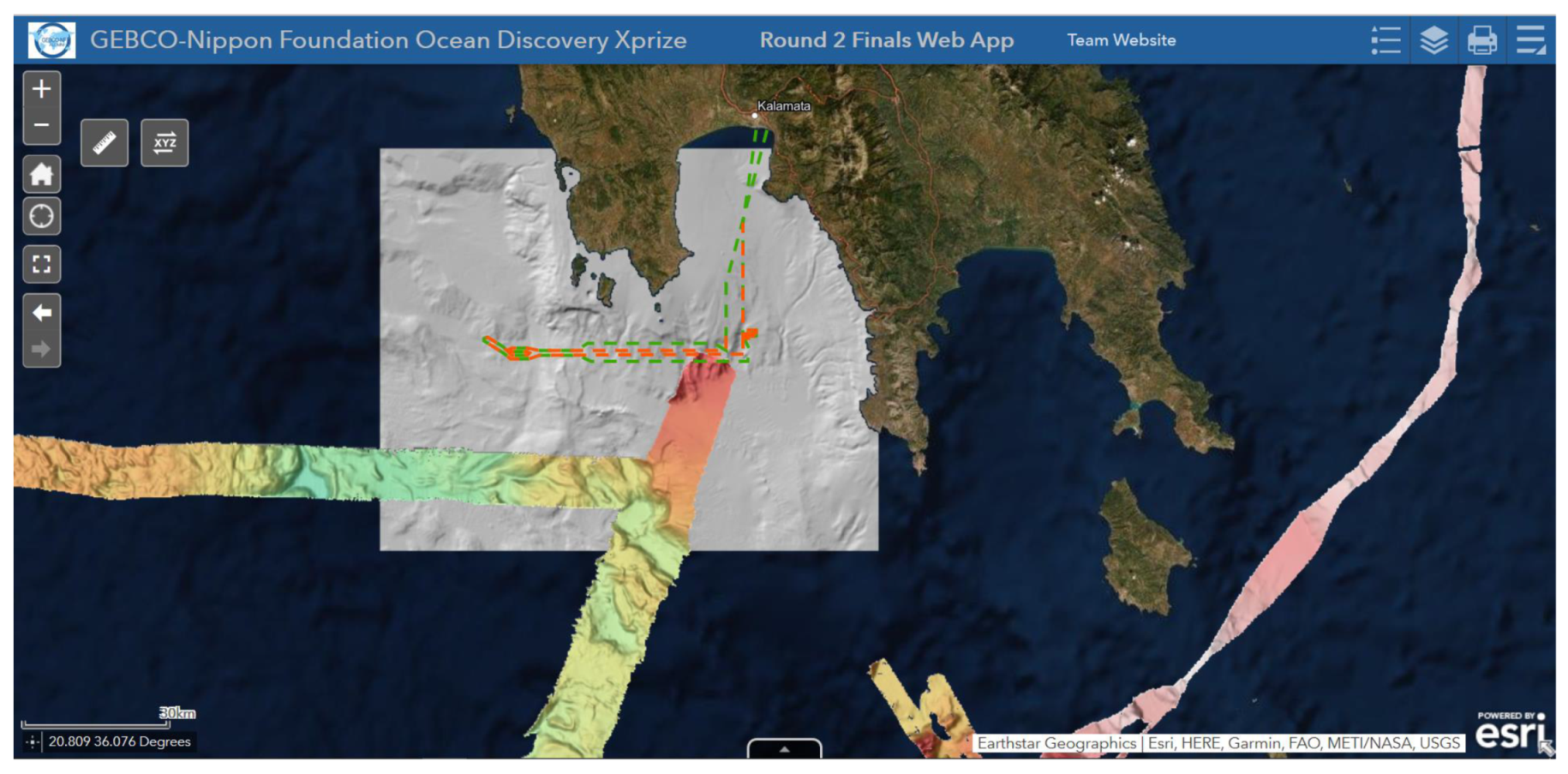
2.2. Mapping Area
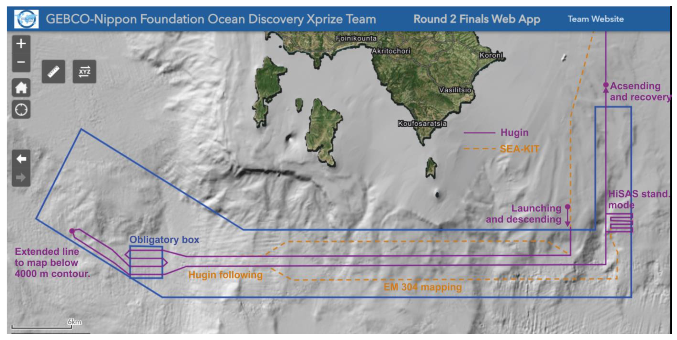
2.3. Survey Plan
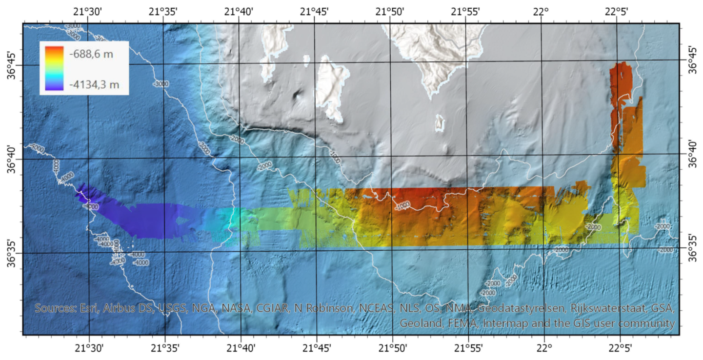
3. Results
3.1. Data Collected
3.2. Data Processing
- Navigation and HISAS: HISAS was tightly integrated with the Aided Inertial Navigation of the HUGIN AUV and uses 4D Kalman filtering to process the raw data into bathymetry and imagery of the sea floor. Prior to processing the HISAS data, Navlab was utilized to generate a navigation solution [26] by injecting real-time transponder interrogations into the vehicle navigation algorithm. The navigation was then re-run through a Kalman filter, prior to running a smoothing algorithm on the output. In addition to the navigation processing, the depth was calculated using a UNESCO pressure to depth calculation [27], based on conductivity and temperature information extracted during the ascent and descent of the AUV during the mission. The output was a smoothed navigation file, containing all information relevant to the navigation of the vehicle within the mission, such as time, position, depth, attitude, etc. Once the navigation solution was generated, NEXUS software was used to communicate with the FOCUS machine to process the HISAS 1032 records, using the raw stave data to generate bathymetry and sidescan using the optimal navigation solution.
- Bathymetry: CARIS HIPS and SIPS were utilized to process the EM 2040, HISAS, and EM 304 data. The Process Designer tool was used by the team to create process models, which were used to reduce processing times. The process models were used to merge the raw sonar data, sound velocity data, smoothed navigation data, and tide information used to produce bathymetric surfaces and side scan mosaics.
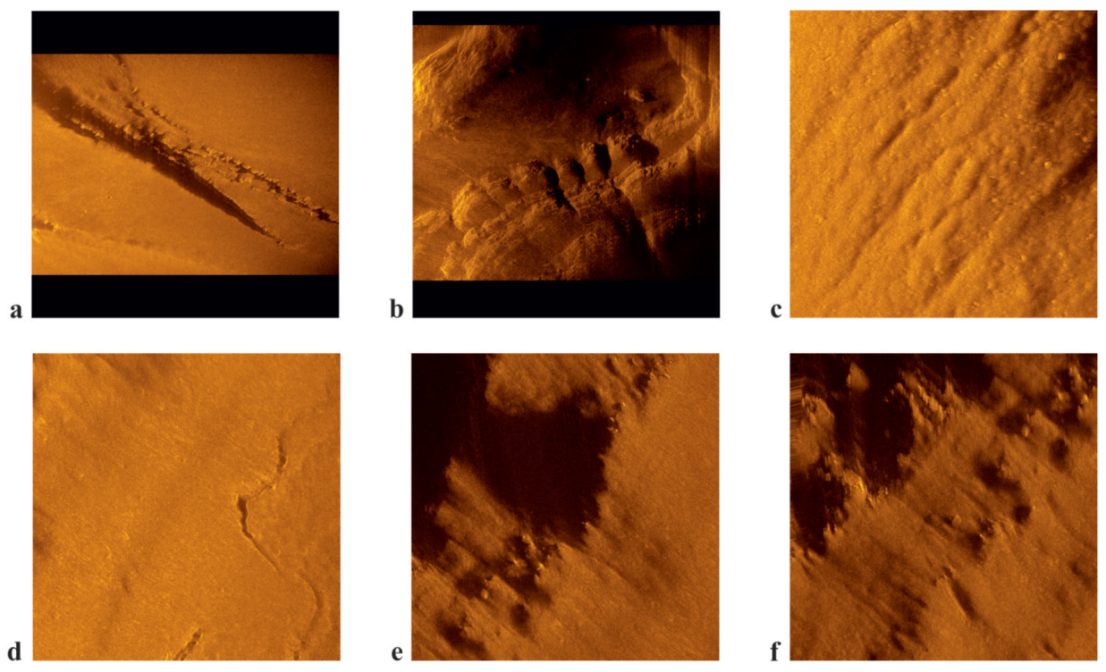
- Imagery: EM 304 data were uploaded to the cloud, for remote data processing using Qimera and Fledermaus to process data and produce point cloud images and imagery of the sea floor. Ultra-high resolution acoustic images were generated on site from the HISAS data, using REFLECTIONS software to produce 2-cm resolution, spot processed images.
- ArcGIS Visualization: When the processing was complete, all the combined bathymetric data were presented to the Shell Ocean Discovery XPRIZE representatives using the team’s ArcGIS online portal. Prior to publishing in the online account, all of the processed data were integrated within an ArcGIS Desktop map document. Vector datasets were published to an ArcGIS feature services. Raster products (bathymetric maps and imagery) were published to ArcGIS Image Services using Earth Analytic’s SmartOcean ArcGIS Enterprise Server Cluster. The datasets could then be manipulated using various functions such as hillshade, slope, aspect, and elevation. The mosaic datasets were published as ArcGIS image services and added to the final ArcGIS WebMap, which was in turn embedded in a customized web application. This application included ’pop-ups’ showing imagery linked to specific geographic locations.
4. Discussion
4.1. Uncertainty Estimation and Error Budget
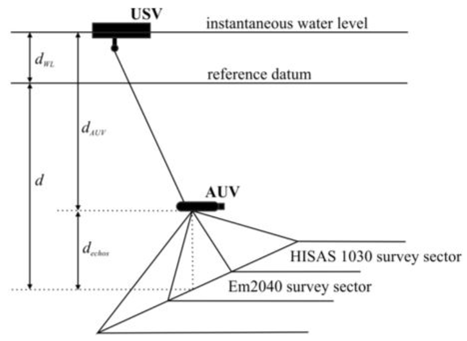
4.1.1. Vertical Uncertainty Estimation
Measurements by AUV HUGIN
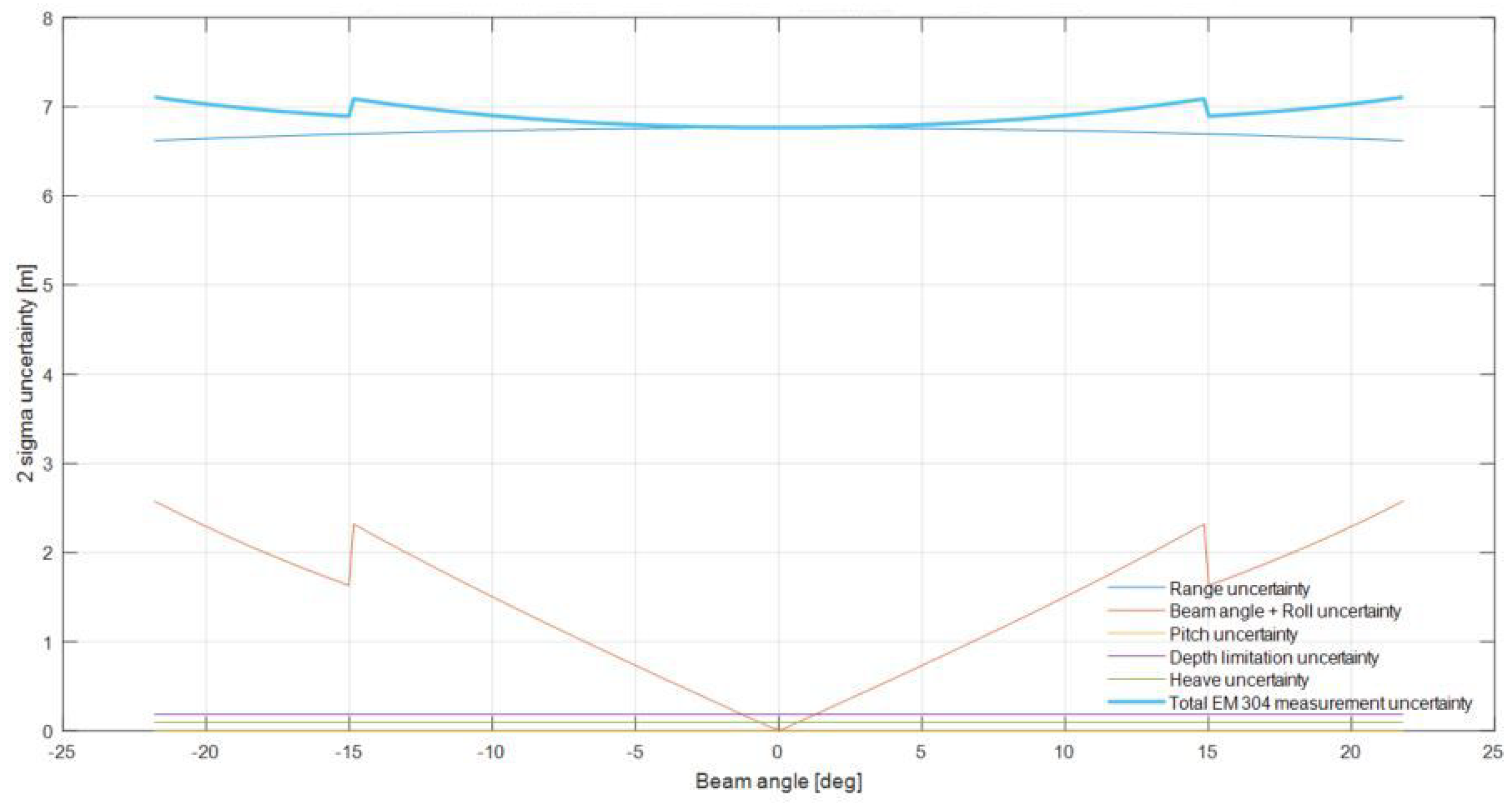
Measurement by USV SEA-KIT
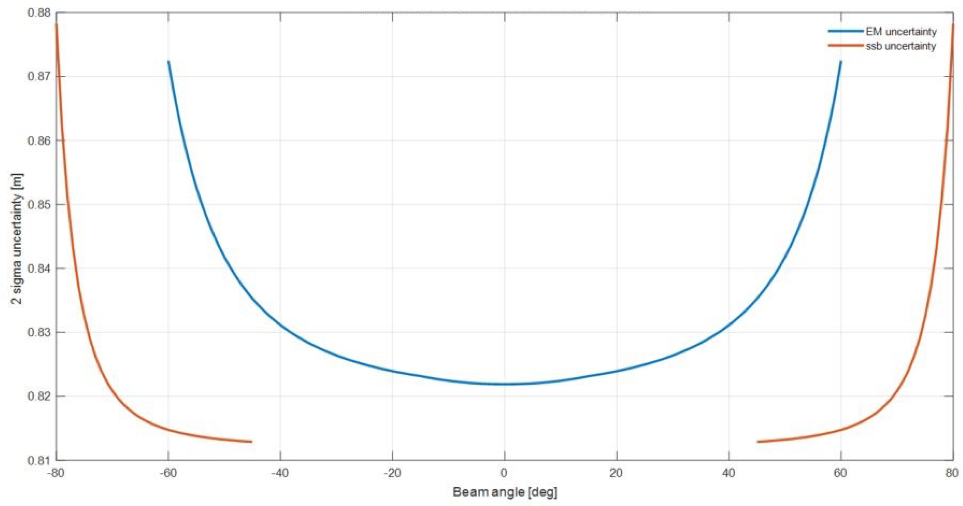
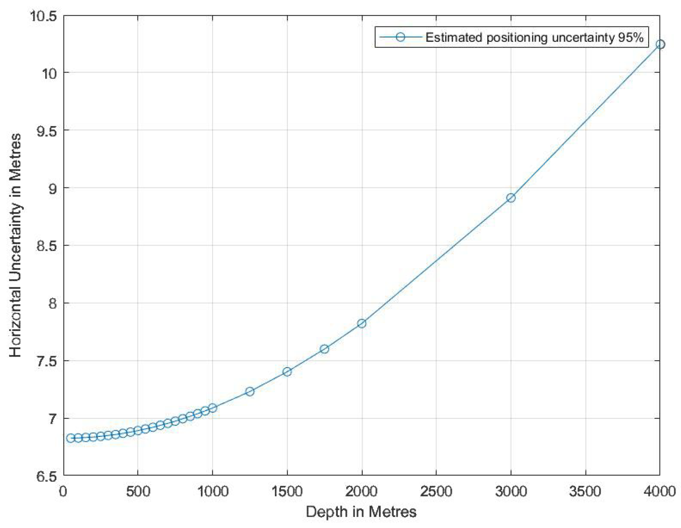
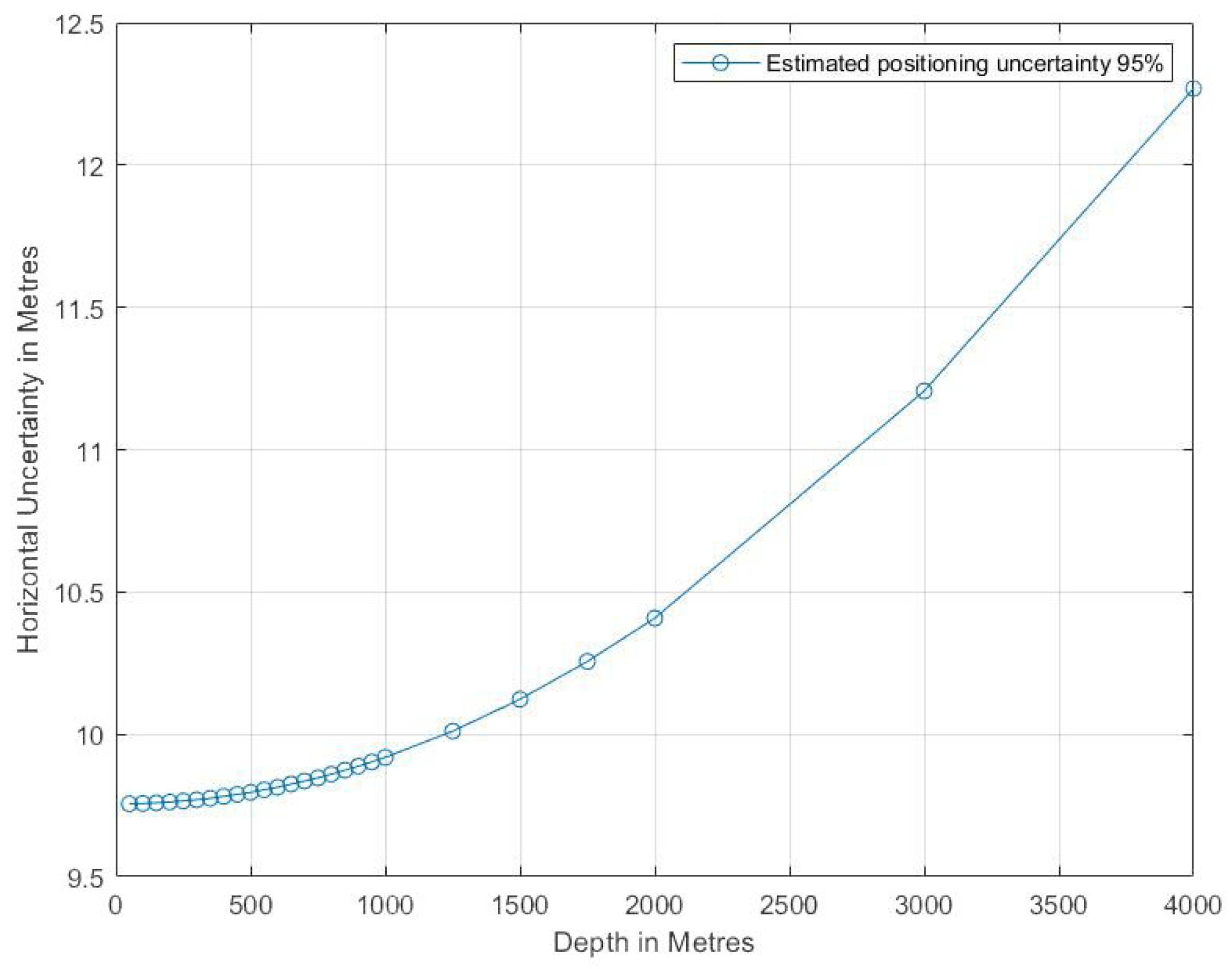
4.1.2. Horizontal Uncertainty Estimation
- GPS accuracy;
- USBL measurement accuracy;
- surface ship attitude errors/measurement errors; and
- sound velocity errors.
4.2. Mapping Resolution
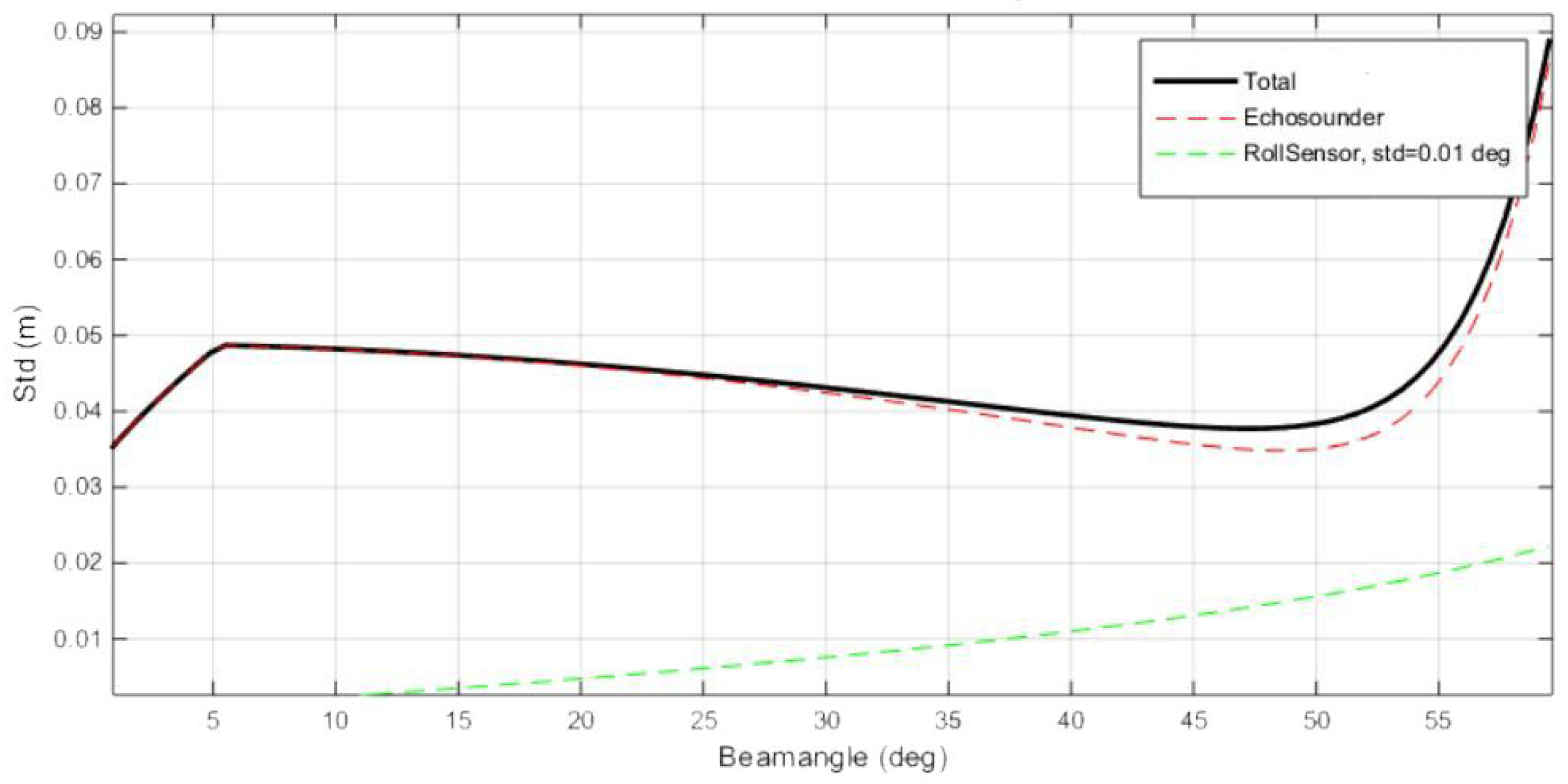
4.2.1. Vertical Mapping Resolution
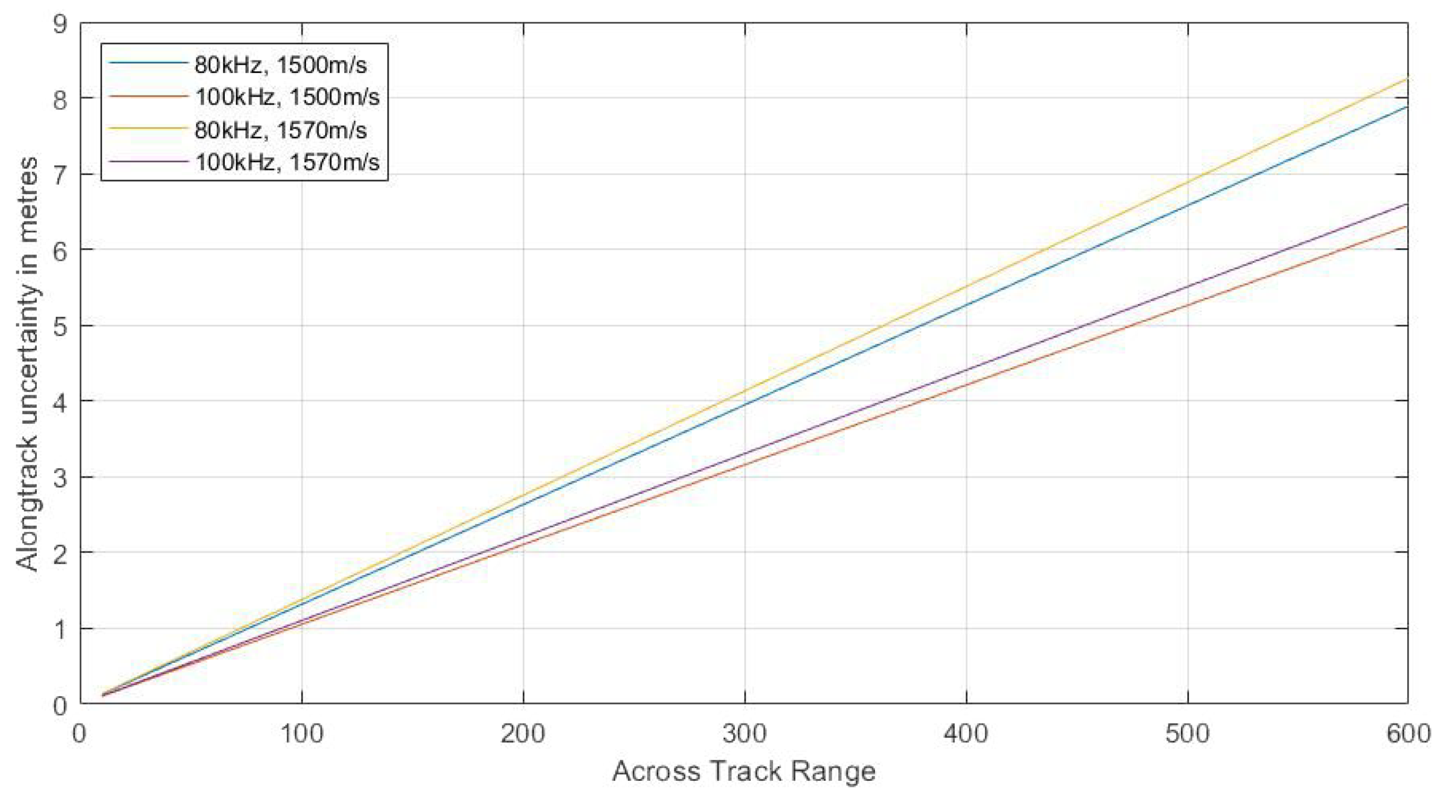
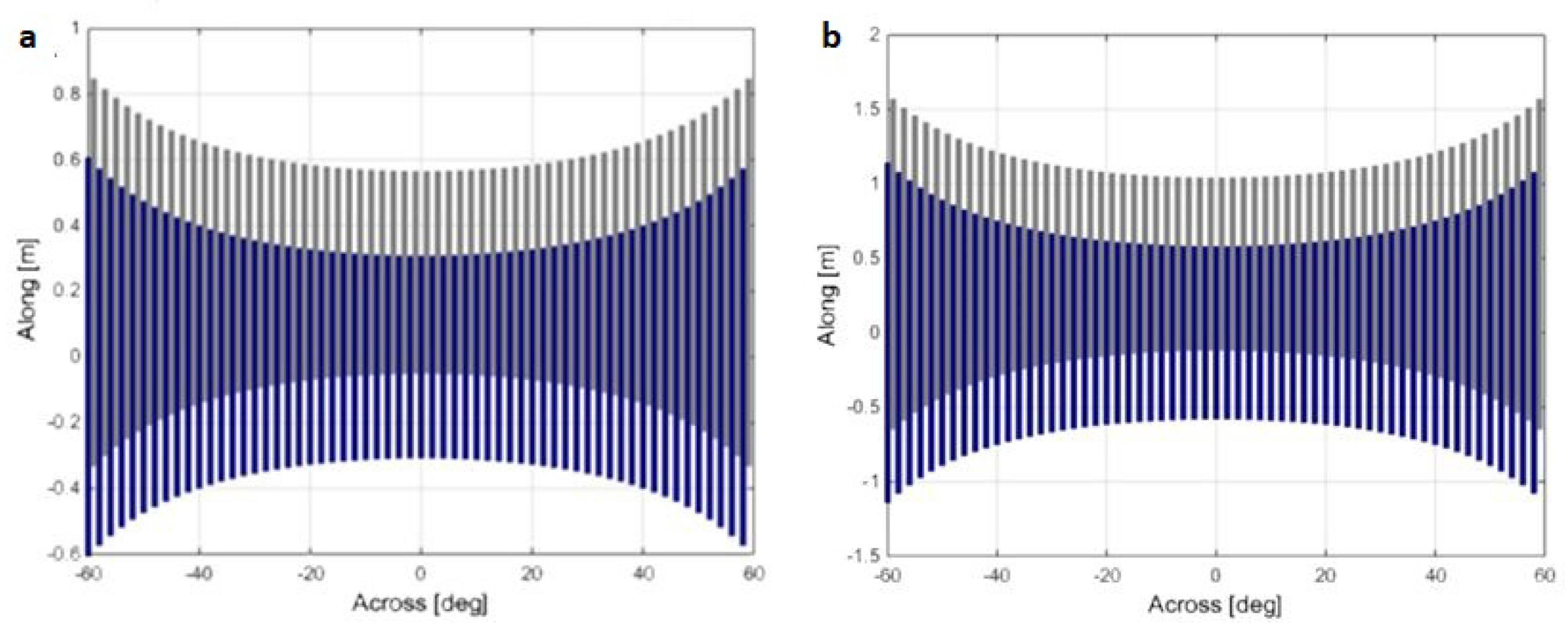
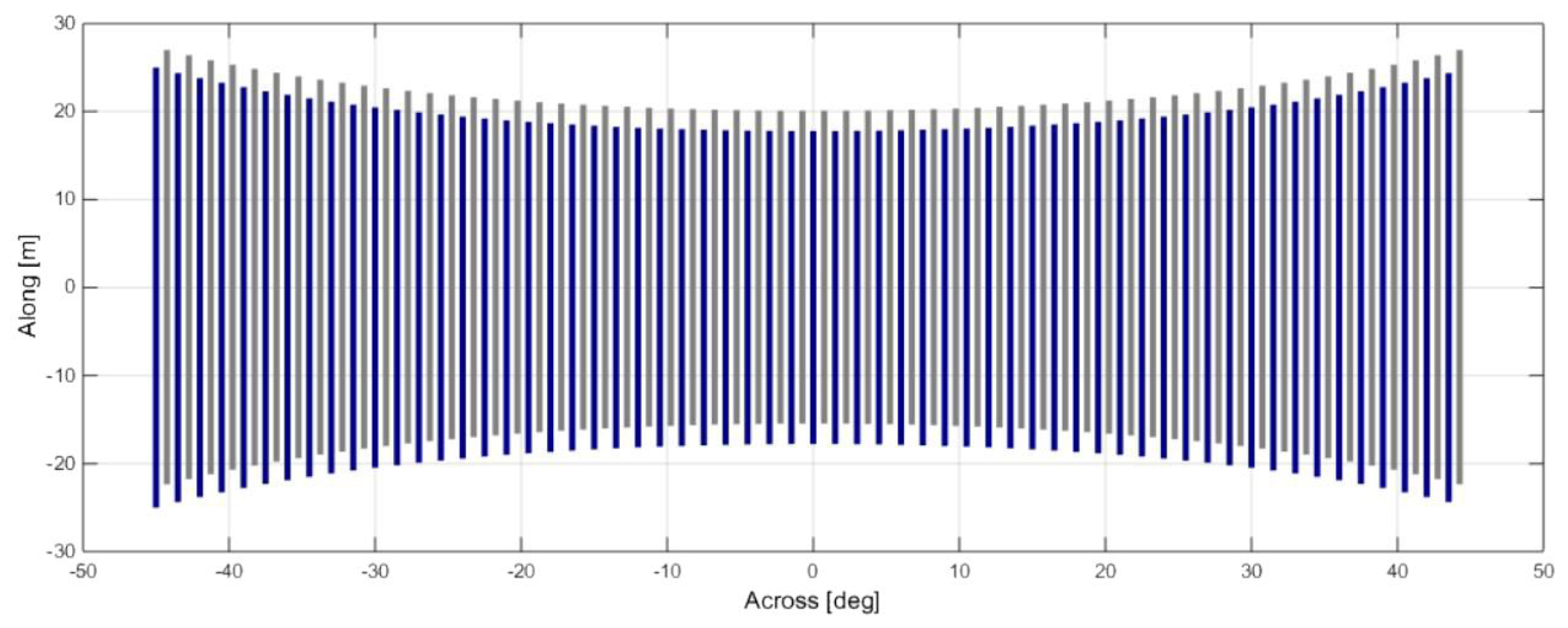
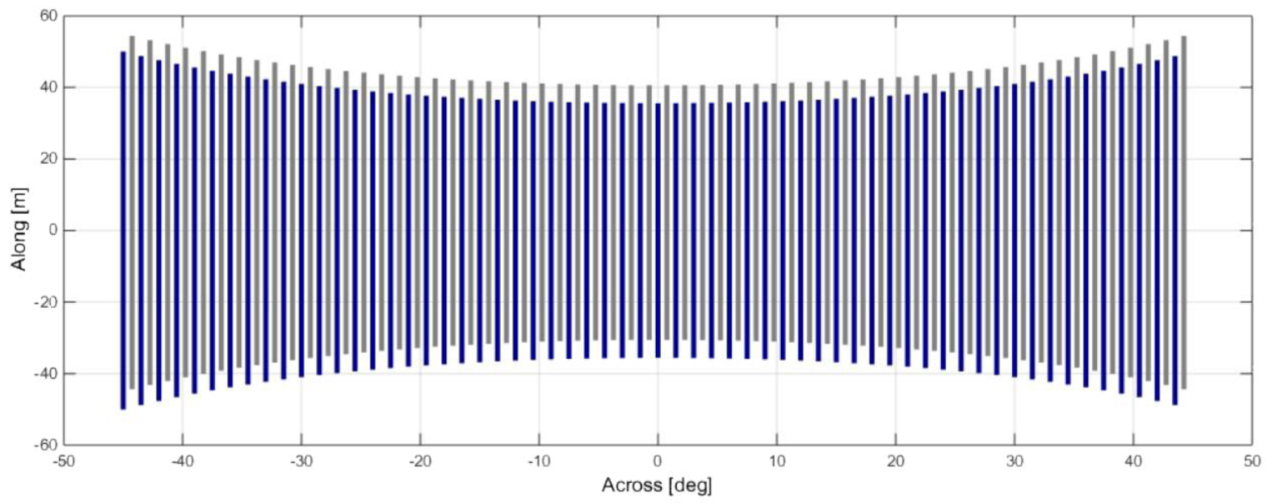
4.2.2. Horizontal Mapping Resolution
1032 Wide Area Mode
HISAS 1032 Standard Mode
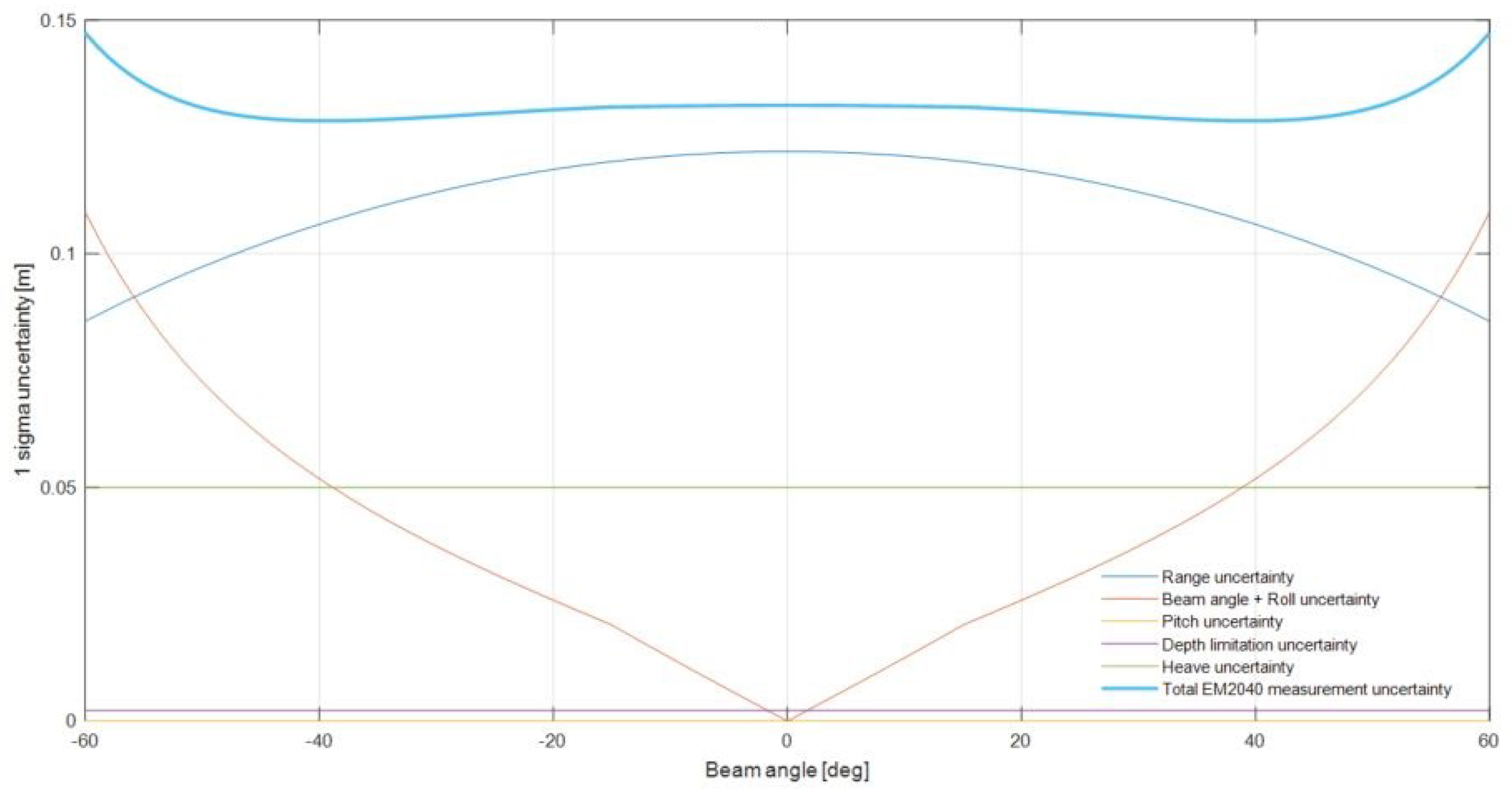
EM 2040
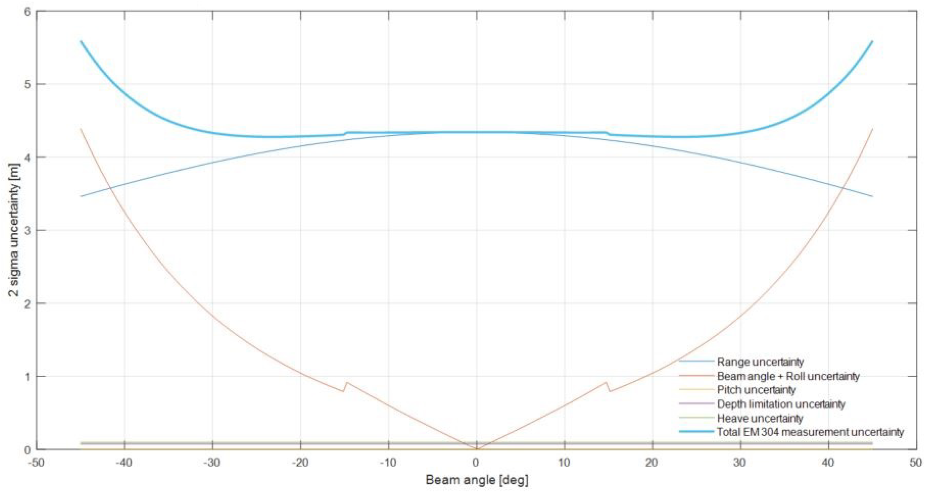
EM 304
4.3. The Assessment of AUV Performance While Cooperating with USV
5. Conclusions
Supplementary Materials
Author Contributions
Funding
Acknowledgments
Conflicts of Interest
Abbreviations
| AUV | Autonomous Underwater Vehicle |
| USV | Unmanned Surface Vessel |
| HISAS | High Resolution Synthetic Aperture Sonar |
| MBES | Multibeam Echosounder |
| USBL | Ultra-short baseline |
| AINS | Augmented Inertial Navigation System |
| IMU | Inertial Measurement Unit |
| CTD | Conductivity, Temperature, Depth |
| OFG | Ocean Floor Geophycisc |
| CCTV | Closed Circuit Television |
| AGM | Absorbent Glass Mat |
| VRLA | Valve Regulated Lead Acid |
| CUBE | Combined Uncertainty and Bathymetry Estimation |
| WL | Water Level |
| KF | Kalman Filter |
| GPS | Global Positioning System |
| DVL | Doppler Velocity Log |
| DTM | Digital Terrain Model |
| HAL | Hybrid Autonomy Layer |
References
- Wölfl, A.C.; Snaith, H.; Amirebrahimi, S.; Devey, C.W.; Dorschel, B.; Ferrini, V.; Huvenne, V.A.I.; Jakobsson, M.; Jencks, J.; Johnston, G.; et al. Seafloor Mapping—The Challenge of a Truly Global Ocean Bathymetry. Front. Mar. Sci. 2019, 6, 283. [Google Scholar] [CrossRef]
- Mayer, L.; Jakobsson, M.; Allen, G.; Dorschel, B.; Falconer, R.; Ferrini, V.; Lamarche, G.; Snaith, H.; Weatherall, P. The Nippon Foundation—GEBCO Seabed 2030 Project: The Quest to See the World’s Oceans Completely Mapped by 2030. Geosciences 2018, 8, 63. [Google Scholar] [CrossRef] [Green Version]
- Smith, W.H.F.; Sandwell, D.T. Bathymetric prediction from dense satellite altimetry and sparse shipboard bathymetry. Pap. Geomagn. Paleomagn. Mar. Geol. Geophys. 1994. [Google Scholar] [CrossRef]
- Wigley, R.; Zarayskaya, Y.; Bazhenova, E.; Falconer, R.; Zwolak, K. Nippon Foundation/GEBCO ocean mapping training program at the University of New Hampshire: 13 years of success and alumni activities. In Proceedings of the OCEANS 2017, Aberdeen, UK, 19–22 June 2017. [Google Scholar] [CrossRef]
- Kristensen, J.; Vestgard, K. Hugin-an untethered underwater vehicle for seabed surveying. In Proceedings of the IEEE Oceanic Engineering Society, OCEANS’98, Conference Proceedings (Cat. No.98CH36259), Nice, France, 28 September–1 October 1998; Volume 1, pp. 118–123. [Google Scholar] [CrossRef]
- Hagen, P.E.; Storkersen, N.; Vestgard, K.; Kartvedt, P. The HUGIN 1000 autonomous underwater vehicle for military applications. In Proceedings of the Oceans 2003, Celebrating the Past...Teaming Toward the Future (IEEE Cat. No.03CH37492), San Diego, CA, USA, 22–26 September 2003; Volume 2, pp. 1141–1145. [Google Scholar]
- Hagen, P.E.; Storkersen, N.; Marthinsen, B.E.; Sten, G.; Vestgard, K. Military operations with HUGIN AUVs: Lessons learned and the way ahead. Eur. Ocean. 2005, 2, 810–813. [Google Scholar]
- Hagen, P.E.; Størkersen, N.; Marthinsen, B.E.; Sten, G.; Vestgård, K. Rapid environmental assessment with autonomous underwater vehicles—Examples from HUGIN operations. J. Mar. Syst. 2008, 69, 137–145. [Google Scholar] [CrossRef]
- Jalving, B.; Gade, K.; Svartveit, K.; Willumsen, A.B.; Sørhagen, R. DVL Velocity Aiding in the HUGIN 1000 Integrated Inertial Navigation System. Model. Identif. Control. 2004, 25, 223–236. [Google Scholar] [CrossRef] [Green Version]
- Kongsberg. Autonomous Underwater Vehicle—AUV. The HUGIN Family. Available online: https://www.kongsberg.com/globalassets/maritime/km-products/product-documents/hugin-family-of-auvs (accessed on 19 April 2020).
- Marthiniussen, R.; Vestgard, K.; Klepaker, R.A.; Storkersen, N. HUGIN-AUV concept and operational experiences to date. In Proceedings of the Oceans ’04 MTS/IEEE Techno-Ocean ’04 (IEEE Cat. No.04CH37600), Kobe, Japan, 9–12 November 2004; Volume 2, pp. 846–850. [Google Scholar]
- Proctor, A.A.; Zarayskaya, Y.; Bazhenova, E.; Sumiyoshi, M.; Wigley, R.; Roperez, J.; Zwolak, K.; Sattiabaruth, S.; Sade, H.; Tinmouth, N.; et al. Unlocking the Power of Combined Autonomous Operations with Underwater and Surface Vehicles: Success with a Deep-Water Survey AUV and USV Mothership. In Proceedings of the 2018 OCEANS—MTS/IEEE Kobe Techno-Oceans (OTO), Kobe, Japan, 28–31 May 2018. [Google Scholar] [CrossRef]
- Zwolak, K.; Simpson, S.; Anderson, B.; Bazhenova, E.; Falconer, R.; Kearns, T.; Minami, H.; Roperez, J.; Rosedee, A.; Sade, H.; et al. An unmanned seafloor mapping system: The concept of an AUV integrated with the newly designed USV SEA-KIT. In Proceedings of the OCEANS 2017, Aberdeen, UK, 19–22 June 2017. [Google Scholar] [CrossRef]
- Zarayskaya, Y.; Wallace, C.; Wigley, R.A.; Zwolak, K.; Bazhenova, E.; Bohan, A.; Elsaied, M.; Roperez, J.; Sumiyoshi, M.; Sattiabaruth, S.; et al. GEBCO-NF Alumni Team Technology Solution for Shell Ocean Discovery XPRIZE Final Round. In Proceedings of the OCEANS 2019, Marseille, France, 17–20 June 2019. [Google Scholar] [CrossRef]
- Ludvigsen, M.; Johnsen, G.; Lagstad, P.; Sørensen, A.; Odegard, O. Scientific Operations Combining ROV and AUV in the Trondheim Fjord. Mar. Technol. Soc. J. 2013, 48, 1–7. [Google Scholar] [CrossRef]
- Salavasidis, G.; Harris, C.A.; Rogers, E.; Phillips, A.B. Co-operative Use of Marine Autonomous Systems to Enhance Navigational Accuracy of Autonomous Underwater Vehicles. In Towards Autonomous Robotic Systems; Alboul, L., Damian, D., Aitken, J., Eds.; Lecture Notes in Computer Science; Springer: Berlin/Heidelberg, Germany, 2016; Volume 9716. [Google Scholar]
- Sarda, E.I.; Dhanak, M.R. A USV-Based Automated Launch and Recovery System for AUVs. IEEE J. Ocean. Eng. 2017, 42, 37–55. [Google Scholar] [CrossRef]
- Hansen, R.E. Mapping the ocean floor in extreme resolution using interferometric synthetic aperture sonar. Proc. Meet. Acoust. ICU 2019, 38, 055003. [Google Scholar] [CrossRef] [Green Version]
- Jacobs, T. Search for Flight MH 370 Shows Durability of AUVs. E&P Notes 2016. [Google Scholar] [CrossRef]
- Enzmann, R. Ocean Infinity in the Search for The Lost. Argentinian Submarine, ARA San Juan. ROVplanet 2019, 3, 39–42. [Google Scholar]
- Meng, L.; Gu, H.; Lin, Y.; Bai, G.; Tang, D. Study on the Mechanical Characteristics of a Towing Docking Device for USV Self-Recovering AUVs. In Proceedings of the OCEANS 2019, Marseille, France, 17–20 June 2019; pp. 1–8. [Google Scholar] [CrossRef]
- Gu, H.; Meng, L.; Tang, D.; Li, N.; Wang, Z.; Bai, G.; Liu, S.; Zhang, H.; Lin, Y. The Lake Trial about the Autonomous Recovery of the UUV by the USV Towed System. In Proceedings of the OCEANS 2019, Marseille, France, 17–20 June 2019; pp. 1–7. [Google Scholar] [CrossRef]
- Zwolak, K.; Zarayskaya, Y.; Wigley, R.; Lacerda, C.; Ketter, T.; Anderson, R.; Bazhenova, E.; Bohan, A.; Dorshow, W.; Elsaied, M.; et al. The Shell Ocean Discovery Xprize Competition Impact on the Development of Ocean Mapping Possibilities. Annu. Navig. 2018, 25, 125–136. [Google Scholar] [CrossRef] [Green Version]
- Calder, B.R.; Mayer, L.A. Automatic Processing of High-Rate, High-Density Multibeam Echosounder Data. Geochem. Geophys. Geosyst. 2003, 4. [Google Scholar] [CrossRef]
- Calder, B.R.; Wells, D.E. CUBE User’s Manual. Center for Coastal and Ocean Mapping. 1217. 2007. Available online: https://scholars.unh.edu/ccom/1217 (accessed on 19 April 2020).
- Gade, K. NavLab, a Generic Simulation and Post-processing Tool for Navigation. Model. Identif. Control. Nor. Soc. Autom. Control. 2005, 26, 135–150. [Google Scholar] [CrossRef]
- UNESCO. UNESCO: Algorithms for Computation of Fundamental Properties of Seawater; UNESCO Technical Papers in Marine Science; UNESCO: Paris, France, 1983; Volume 44, pp. 1–55. [Google Scholar]
- Minami, H. Estimation of Total Vertical Uncertainty for the Bathymetry Acquired by Autonomous Underwater Vehicle in Deep Water; Report of Hydrographic and Oceanographic Researches No. 50; Hydrographic Survey Division: Miyagi, Japan, 2013.
- Hare, R.; Godin, A.; Mayer, L.A. Accuracy Estimation of Canadian Swath (Multi-Beam) and Sweep (Multi-Transducer) Sounding Systems; Technical Report; Canadian Hydrographic Service: Ottawa, QC, Canada, 1995. [Google Scholar]
- Saebo, T.O. Seafloor Depth Estimation by means of Interferometric Synthetic Aperture Sonar. Ph.D. Thesis, University of Tromso, Tromso, Norway, 2010. [Google Scholar]
- Van Trees, H.L. Optimum Array Processing. Part IV of Detection, Estimation, and Modulation Theory; John Wiley & Sons: New York, NY, USA, 2002. [Google Scholar]
- Hegrenaes, O.; Saebo, T.O.; Hagen, P.E.; Jalving, B. Horizontal Mapping Accuracy in Hydrographic AUV Surveys. In Proceedings of the IEEE AUV Conference, Monterey, CA, USA, 20–23 September 2010. [Google Scholar]
- Hiller, T.; Reed, T.B.; Steingrimsson, A. Producing chart data from interferometric sonars on small AUVs. Int. Hydrogr. Rev. 2011. Available online: http://www.oicinc.com/res/pdf/USHydro_Abstract_Producing-Chart-Data.pdf (accessed on 19 April 2020).
- Lurton, X. An Introduction to Underwater Acoustics. Principles and Applications; Springer: Berlin/Heidelberg, Germany, 2002. [Google Scholar]
- Ocean News & Technology, Swire Seabed Completes Unmanned Subsea Pipeline Inspection for Equinor. Published: 19 August 2019. Available online: https://www.oceannews.com/news/subsea-intervention-survey/swire-seabed-completes-unmanned-subsea-pipeline-inspection-for-equinor (accessed on 2 March 2020).


| Feature | Data |
|---|---|
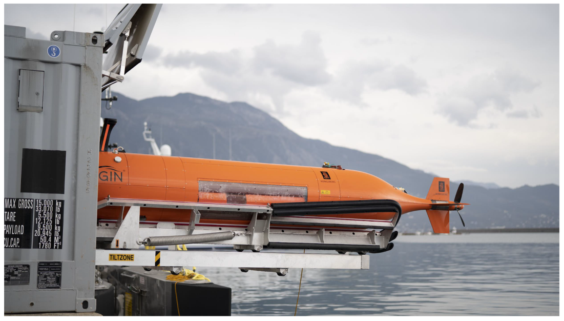
| Dimensions | Length: 6.9 m, diameter: 750 mm, weight: 1200 kg (estimated), speed: 2–6 kn |
| Depth ratings | 4500 m |
| Communication | HiPAP USBL system providing Acoustic Command |
| Data and Emergency Link Functionality | |
| Radio Link—ELPRO 455U, 2–4 km range | |
| Wireless LAN250 | |
| Iridium Satellite Link | |
| Visual Relocation Xenon flash beacon on vehicle body and on vehicle nose | |
| Navigation | NavP Aided Inertial Navigation System (AINS) |
| MGC R3 Inertial Measurement Unit (IMU) | |
| 500 kHz Nortek Doppler velocity log | |
| Digiquarz depth sensor | |
| Forward looking Sonar (Obstacle Avoidance System) | |
| UTP Navigational Capability | |
| Terrain Navigation Module | |
| Payload | HISAS 1032 |
| EM 2040 Multibeam Echosounder | |
| PipeTracker | |
| Camera (CathX—10 Megapixel native resolution) and LED Strobes | |
| CathX Laser system | |
| Edgetcth 2205 SBP 2–16 kHz | |
| OFG SCM Magnetometer | |
| SAIV CTD | |
| Environmental Package including: | |
| Contros Co2, Contros PAH, METS, HydroFlash O2, FLNTU |
| Feature | Data |
|---|---|
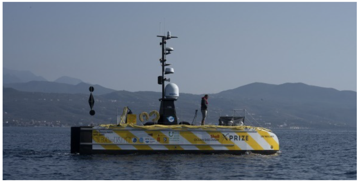
| Dimensions | Length: 11.75 m, beam: 2.2 m, transport height: 2.0 m, operational height: 8.5 m, weight: 12,000 kg (estimated) |
| Communication | Fully redundant communication system: WiFi, Radio |
| Satellite (Iridium and Inmarsat) | |
| Kongsberg Maritime Broadband Radio (<45 km offshore) | |
| CCTV: 2 interior and 6 fore and aft cameras, 360 degree FLIR camera | |
| Propulsion | 2 × 10 kW/1200 rpm electric directional thrust motors |
| Power supply | Generator 2 × 18 kW 48V DC, fuel 2000 l |
| 56 Gel and Absorbent Glass Mat (AGM) types | |
| of valve-regulated lead-acid battery (VRLA) Marine Batteries | |
| 12 V–214 Ah capacity | |
| 4 dry cell Absorbed Glass Matt (AGM) VRLA 12 V 100Ah | |
| Marine Dual Purpose Batteries for the engine and propulsion | |
| Payload | EM 304 Multibeam Echosounder - pre-release version |
| HiPAP 502 High Precision Acoustic Positioning System | |
| Kongsberg Seatex MGC-R3-SB50 motion sensor and gyro compass | |
| sound velocity probe |
| Easting [m] | Northing [m] | Latitude [N] | Longitude [ E] | |
|---|---|---|---|---|
| 1 | 540,222.1 | 4,056,141.2 | 36.65 | 21.45 |
| 2 | 553,120.4 | 4,048,232.9 | 36.58 | 21.59 |
| 3 | 599,597.5 | 4,048,815.4 | 36.58 | 22.11 |
| 4 | 599,355.0 | 4,068,167.3 | 36.75 | 22.11 |
| 5 | 595,352.6 | 4,068,119.8 | 36.75 | 22.07 |
| 6 | 595,508.6 | 4,055,864.7 | 36.64 | 22.07 |
| 7 | 560,327.1 | 4,055,423.7 | 36.64 | 21.68 |
| 8 | 544,645.0 | 4,065,037.6 | 36.73 | 21.50 |
| Easting [m] | Northing [m] | Latitude [N] | Longitude [E] | |
|---|---|---|---|---|
| 1 | 549,583.2 | 4,053,524.3 | 36.625968 | 21.554558 |
| 2 | 552,745.5 | 4,053,524.2 | 36.625798 | 21.589924 |
| 3 | 552,745.5 | 4,050,362.0 | 36.597292 | 21.589707 |
| 4 | 549,582.9 | 4,050,361.9 | 36.597461 | 21.554350 |
| Mapping Equipment | Survey Speed [kn] | Height above the Seafloor [m] | Max. Swath (Approximate) [m] |
|---|---|---|---|
| HUGIN—HISAS wide area mode | 3.5 | 70 | 1000 |
| HUGIN—HISAS standard mode | 3.5 | 40 | 350 |
| SEA-KIT—EM 304 | 3.5–4.2 | surface vessel | 2000 |
| multibeam echosounder |
| Data Type | Data Volume |
|---|---|
| Navigation and vehicle health from the CP | 40 GB |
| Payload data from the PP/NAS (Bathy data) | 22 GB |
| SEA-KIT navigation data | 1 MB |
| EM 304 data from SEA-KIT | 6.5 GB bathy plus 150 GB of water column data |
| NAS bottle (HUGIN collected data) | 958 GB |
| Sonar | File Type | Data Type | Resolution [m] | Survey Time [h] | Survey Speed [kn] | Full Swath Width [km] | Coverage [km] |
|---|---|---|---|---|---|---|---|
| EM 304 | *.kmall | Bathymetry and backscatter | depth dependent | 12.6 | 3.5 | 2 * | 163.3 *** |
| EM 2040 | *.all | Bathymetry and backscatter | <1 | 24 | 3.5 | 0.28 ** | 43.6 |
| HISAS Standard mode | *.all *.xtf | Bathymetry SAS Imagery | 1 0.04 | 2 | 3.5 | 0.35 | 4.5 |
| HISAS Wide-area mode | *.all *.xtf | Bathymetry SAS Imagery | 5 1 | 22 | 3.5 | 1 | 142.6 |
| Total (taking into account the overlaps and some data lost on turns): | 278.9 | ||||||
| Parameter | Value | 2 Uncertainty |
|---|---|---|
| Sound speed | 1500 m/s | 1.2 m/s |
| Surface sound speed | 1500 m/s | 0.6 m/s |
| AUV pitch | 0 | 0.02 (for measurement), |
| 0.1 (for misalignment) | ||
| AUV roll | 0 | 0.02 (for measurement), |
| 0.1 (for misalignment) |
| Parameter | Value | 2 Uncertainty |
|---|---|---|
| Beamwidth | 2 × 4 | - |
| Sound speed | 1500 m/s | 6.0 m/s |
| Surface sound speed | 1500 m/s | 0.04 m/s |
| Vessel pitch | 0 | 0.02 (for measurement), |
| 0.1 (for misalignment) | ||
| Vessel roll | 0 | 0.02 (for measurement), |
| 0.1 (for misalignment) | ||
| Range sampling resolution | 0.46 m | - |
| Pulse length | 5 ms | - |
| Heave measurement uncertainty | 0.05 m | - |
| AUV depth [m] | 50 | 100 | 500 | 1000 | 3000 | 4000 |
| AUV positioning uncertainty [m] | 0.20 | 0.25 | 0.52 | 1.04 | 3.14 | 4.188 |
| AUV depth [m] | 50 | 100 | 500 | 1000 | 3000 |
| AUV positioning uncertainty [m] | 0.12 | 0.13 | 0.17 | 0.28 | 0.75 |
| Source of Error | Value |
|---|---|
| GPS 2D error (DRMS) | 0.1 m |
| USBL measurement error (1) | d = 0.03 m; d = 0.06; d = 0.06 |
| Ship attitude error (1) | d = 0.01 (roll); d = 0.01 (pitch); d = 0.08 (heading) |
| USBL calibration/alignment error (1) | d = 0.0 (roll); d = 0.01 (pitch); d = 0.02 (yaw) |
| Error due to fixed SVP error (1) | d = 0.8 m/s |
| Note: assuming constant 1500 m/s true SVP. |
| AUV depth [m] | 50 | 100 | 500 | 1000 | 3000 | 4000 |
| AUV positioning uncertainty [m] | 0.20 | 0.21 | 0.43 | 0.69 | 1.45 | Est < 2 |
| Data Type | Approximate Vertical Resolution for Middle-Swath Beam Angles [m] |
|---|---|
| HISAS Wide area mode | 0.30 |
| HISAS Standard mode (SAS bathymetry) | 0.23 |
| EM 2040 bathymetry | 0.1 |
| Ground range [m] | 60 | 150 | 240 | 310 | 390 |
| Across track resolution [m] | 3.5255 | 3.4465 | 3.2985 | 3.2594 | 3.2376 |
| Altitude [m] | 40 | 40 | 40 | 75 | 75 | 75 |
|---|---|---|---|---|---|---|
| Beam Pointing Angle [] | 0 | 30 | 60 | 0 | 30 | 60 |
| Alongtrack Footprint | 0.3 | 0.35 | 0.6 | 0.56 | 0.65 | 1.12 |
| Acrosstrack Footprint | 0.69 | 0.69 | 0.69 | 1.3 | 1.3 | 1.3 |
| Altitude | 40 m | 75 m |
|---|---|---|
| Along track Spacing in m | 0.25 | 0.46 |
| Across track Spacing in m | 0.35 | 0.65 |
| Sounding Density 5 m cell | 280.6 | 83.5 |
| Altitude [m] | 1000 | 1000 | 1000 | 1500 | 1500 | 1500 | 2000 | 2000 | 2000 |
|---|---|---|---|---|---|---|---|---|---|
| Beam Pointing Angle [] | 0 | 30 | 60 | 0 | 30 | 60 | 0 | 30 | 60 |
| Alongtrack Footprint [m] | 34.85 | 40.24 | 49.29 | 52.31 | 60.4 | 63.86 | 69.77 | 80.57 | 76.98 |
| Acrosstrack Footprint [m] | 9.24 | 9.24 | 9.24 | 9.71 | 9.71 | 9.71 | 8.6 | 8.6 | 8.6 |
| Altitude | 1000 m | 1500 m | 2000 m |
|---|---|---|---|
| Along track Spacing [m] | 2.19 | 3.26 | 3.76 |
| Across track Spacing [m] | 4.62 | 4.86 | 4.31 |
| Sounding Density 5 m cell | 2.5 | 1.6 | 1.5 |
© 2020 by the authors. Licensee MDPI, Basel, Switzerland. This article is an open access article distributed under the terms and conditions of the Creative Commons Attribution (CC BY) license (http://creativecommons.org/licenses/by/4.0/).
Share and Cite
Zwolak, K.; Wigley, R.; Bohan, A.; Zarayskaya, Y.; Bazhenova, E.; Dorshow, W.; Sumiyoshi, M.; Sattiabaruth, S.; Roperez, J.; Proctor, A.; et al. The Autonomous Underwater Vehicle Integrated with the Unmanned Surface Vessel Mapping the Southern Ionian Sea. The Winning Technology Solution of the Shell Ocean Discovery XPRIZE. Remote Sens. 2020, 12, 1344. https://0-doi-org.brum.beds.ac.uk/10.3390/rs12081344
Zwolak K, Wigley R, Bohan A, Zarayskaya Y, Bazhenova E, Dorshow W, Sumiyoshi M, Sattiabaruth S, Roperez J, Proctor A, et al. The Autonomous Underwater Vehicle Integrated with the Unmanned Surface Vessel Mapping the Southern Ionian Sea. The Winning Technology Solution of the Shell Ocean Discovery XPRIZE. Remote Sensing. 2020; 12(8):1344. https://0-doi-org.brum.beds.ac.uk/10.3390/rs12081344
Chicago/Turabian StyleZwolak, Karolina, Rochelle Wigley, Aileen Bohan, Yulia Zarayskaya, Evgenia Bazhenova, Wetherbee Dorshow, Masanao Sumiyoshi, Seeboruth Sattiabaruth, Jaya Roperez, Alison Proctor, and et al. 2020. "The Autonomous Underwater Vehicle Integrated with the Unmanned Surface Vessel Mapping the Southern Ionian Sea. The Winning Technology Solution of the Shell Ocean Discovery XPRIZE" Remote Sensing 12, no. 8: 1344. https://0-doi-org.brum.beds.ac.uk/10.3390/rs12081344