A Conceptual Approach to Modeling the Geospatial Impact of Typical Urban Threats on the Habitat Quality of River Corridors


Abstract
:
1. Introduction
2. Methods
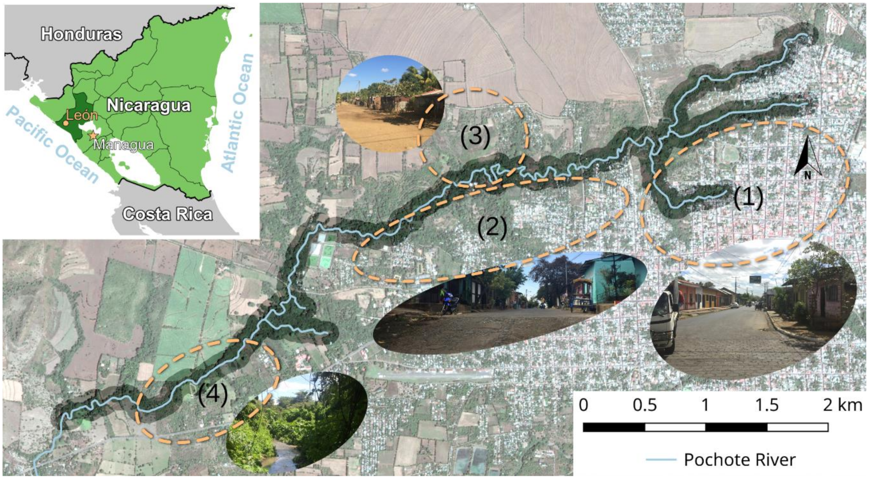
2.1. Study Area
2.2. Methods
2.2.1. Land Use and Land Cover
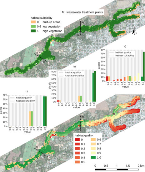
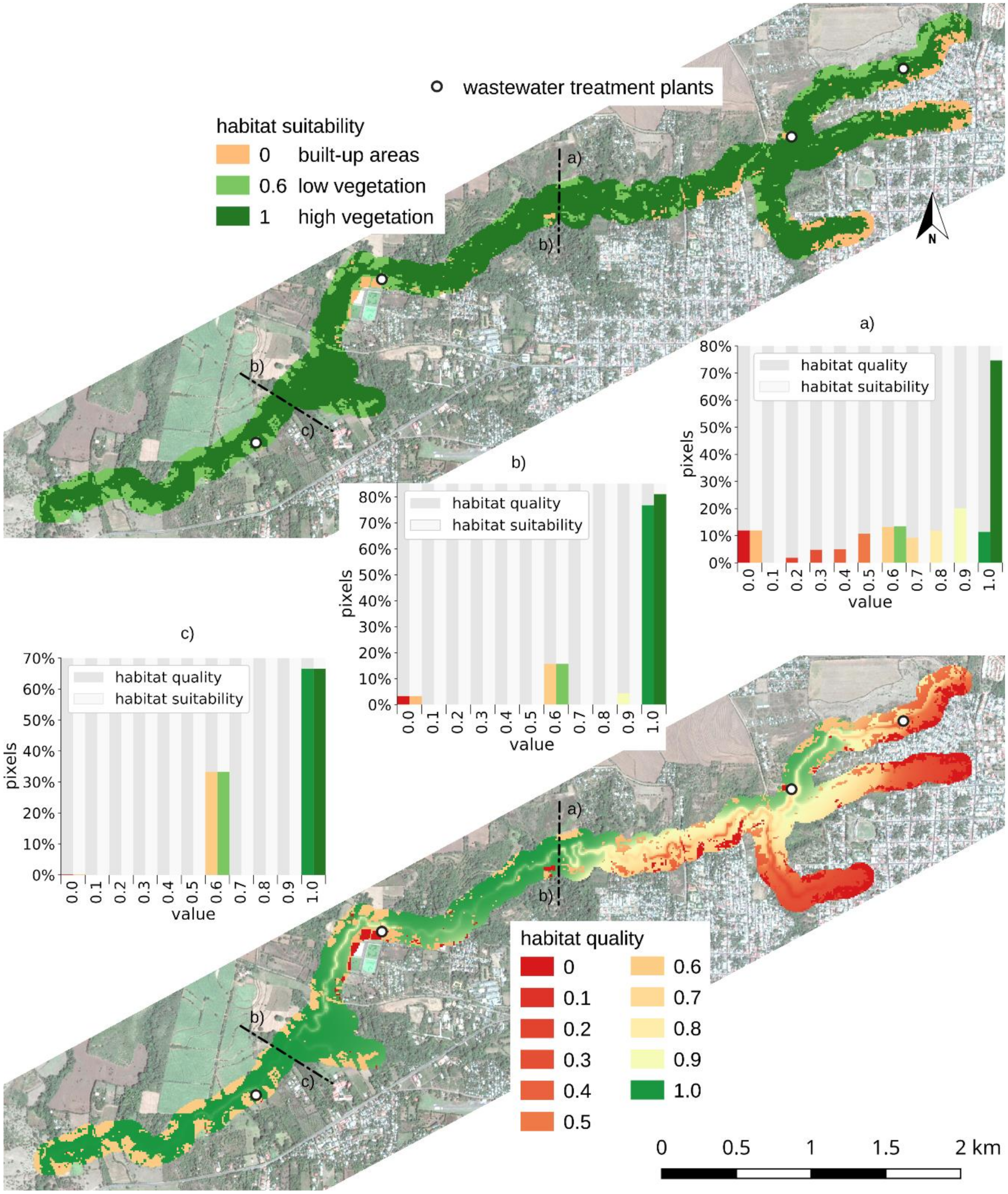
2.2.2. Habitat Suitability
2.2.3. Threat Parameters
- The weight of each threat indicates its relative impact. The weight can have any value between 0 and 1. A weighting score of 1 in a raster map cell causes represents twice as much degradation as a weight score of 0.5 [13].
- The distance and impact of each threat over space. The impact of a threat depends on how quickly it decreases over space. For this case study, an exponential function described this decay, which is an indicative pattern seen in ecology [13]. The impact of a threat r from the threat source raster cell y on a habitat in the raster cell x is given by ixy. The linear distance between cells x and y is dxy and the maximum distance of threat r’s reach is dr,max. The program computes the impact of each threat over space with the following exponential equation [18]:
- The level of accessibility in each habitat cell x. The greater the physical, social, or legal protection the cell has, the less it is affected by threats. Difficult terrain or formal protection are factors that decrease the accessibility [13]. For this case study, the accessibility score was binary, where 1 indicates full accessibility and 0 indicates full protection without any access.
- The relative sensitivity of each habitat type to each threat. The model assumes that the more sensitive a habitat is to a threat, the more it will be affected by it. For example, a forest may suffer more from the proximity of agriculture than of settlements [13]. The sensitivity score for each raster cell ranges between 0 and 1, where 1 indicates the highest sensitivity score [18].
- Dxj: total threat level
- r: threat
- y: indexes all cells on threat r’s raster
- Yr: set of grid cells on threat r’s raster
- Wr: weight of each threat
- irxy: impact of each threat
- βx: level of accessibility in grid cell x
2.2.4. Habitat Quality
- xj: quality of habitat in cell x of habitat type j
- Hj: habitat suitability score of the LULC type j
- : total threat level
- z and k: scaling parameters.
2.2.5. Calculation of Habitat Degradation Due to Threats
- R: habitat degradation due to the impact of all threats
- H: habitat suitability
- Q: habitat quality as a result of all threat impacts
- Rr: habitat degradation due to the impact of threat r
- Qr: habitat quality as a result of threat r.
2.3. Material Used and Model Parameterization
- Current raster LULC map: A GeoTIFF-file raster dataset with a LULC class code for each cell.
- CSV-table with threat data: The CSV-table contains information on the threat’s weight, the maximum distance in kilometers, and information on whether the decay is linear or exponential. For this study, an exponential decay was used.
- Threat raster maps: GeoTIFF-files of the spatial distribution of each threat. Each raster cell contains a value that indicates its presence or absence. The types of threats vary between the current situation and the scenario; therefore, they have their own set of threat raster maps.
- CSV-table with habitat suitability and sensitivity scores: The LULC types, their suitability scores, and the sensitivity of each habitat type to each threat are listed in a CSV-table [18].
- Constant k: The value of the parameter k in Equation (3) is set to the half of the highest grid cell degradation score on the landscape. When running the model, a habitat quality and a habitat degradation raster map is created. The model has to be run once where k is set to 0.5. The model is then run a second time with the new k constant.
Model Parameterization
3. Results
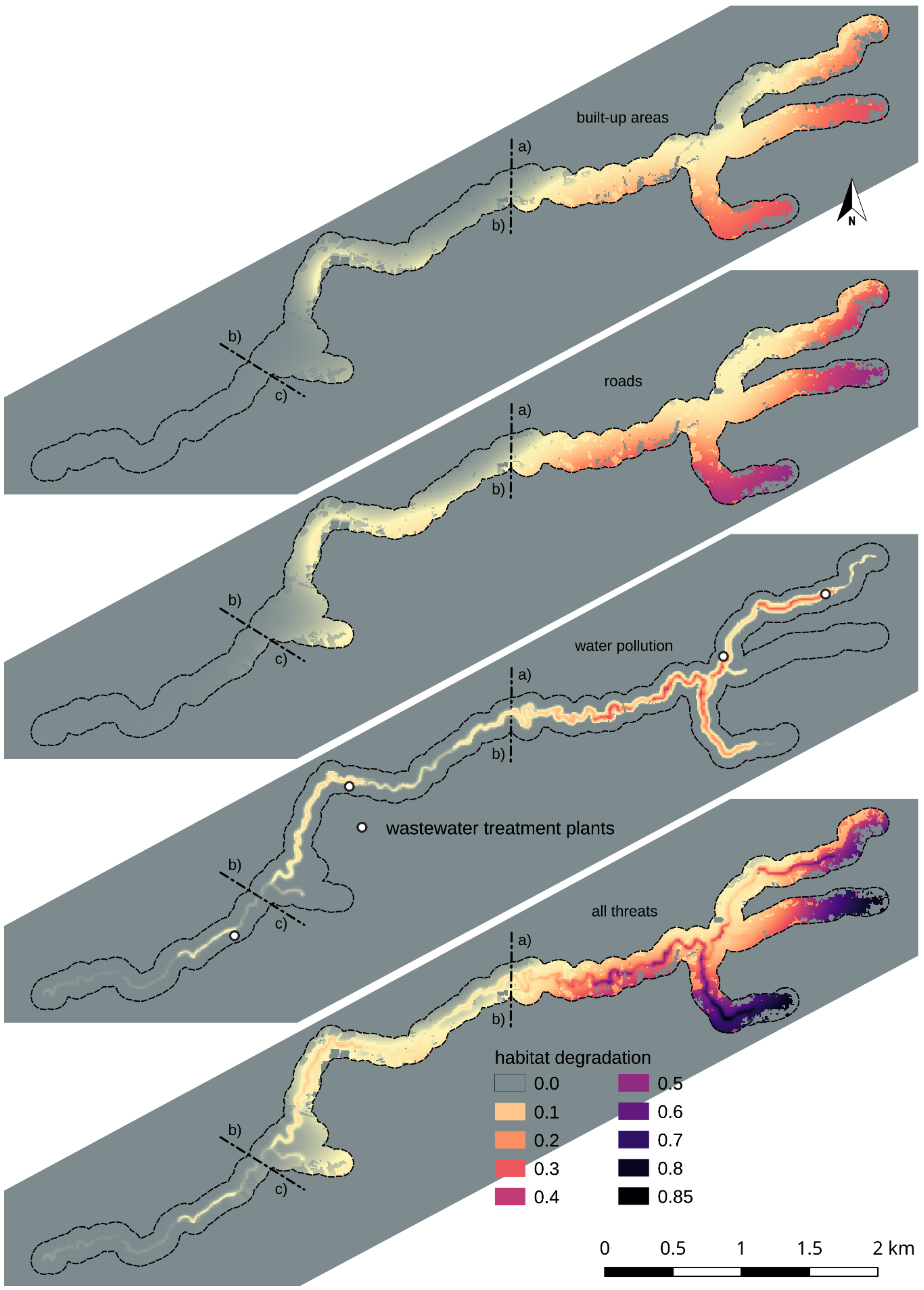
3.1. Habitat Degradation Due to Different Threats
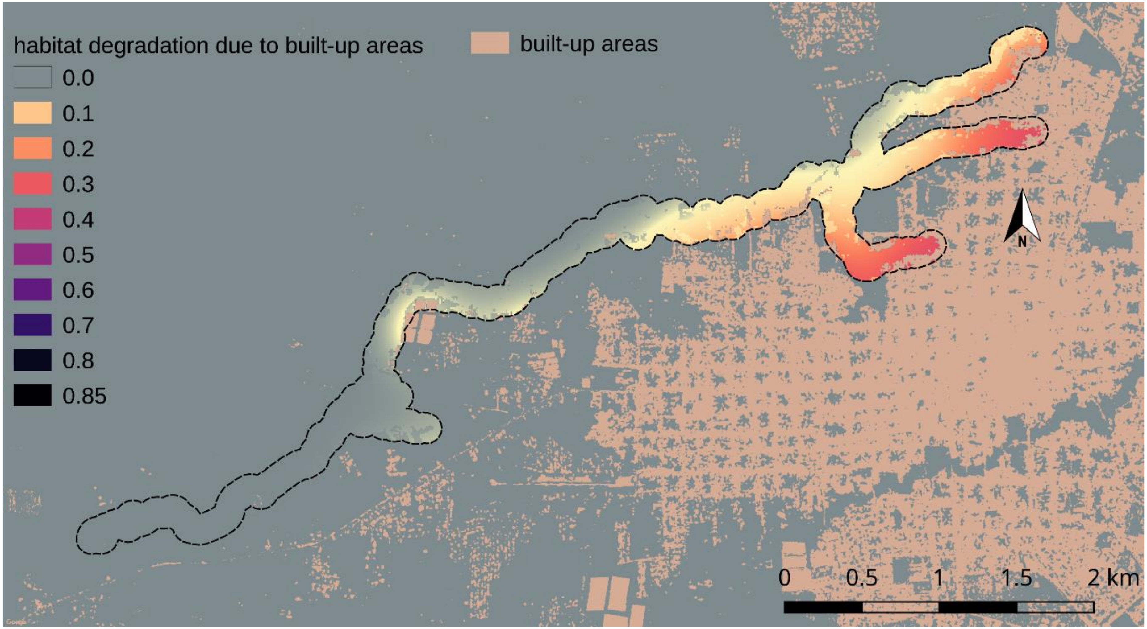
3.1.1. Habitat Degradation Due to Built-Up Areas
3.1.2. Habitat Degradation Due to First- and Second-Order Roads
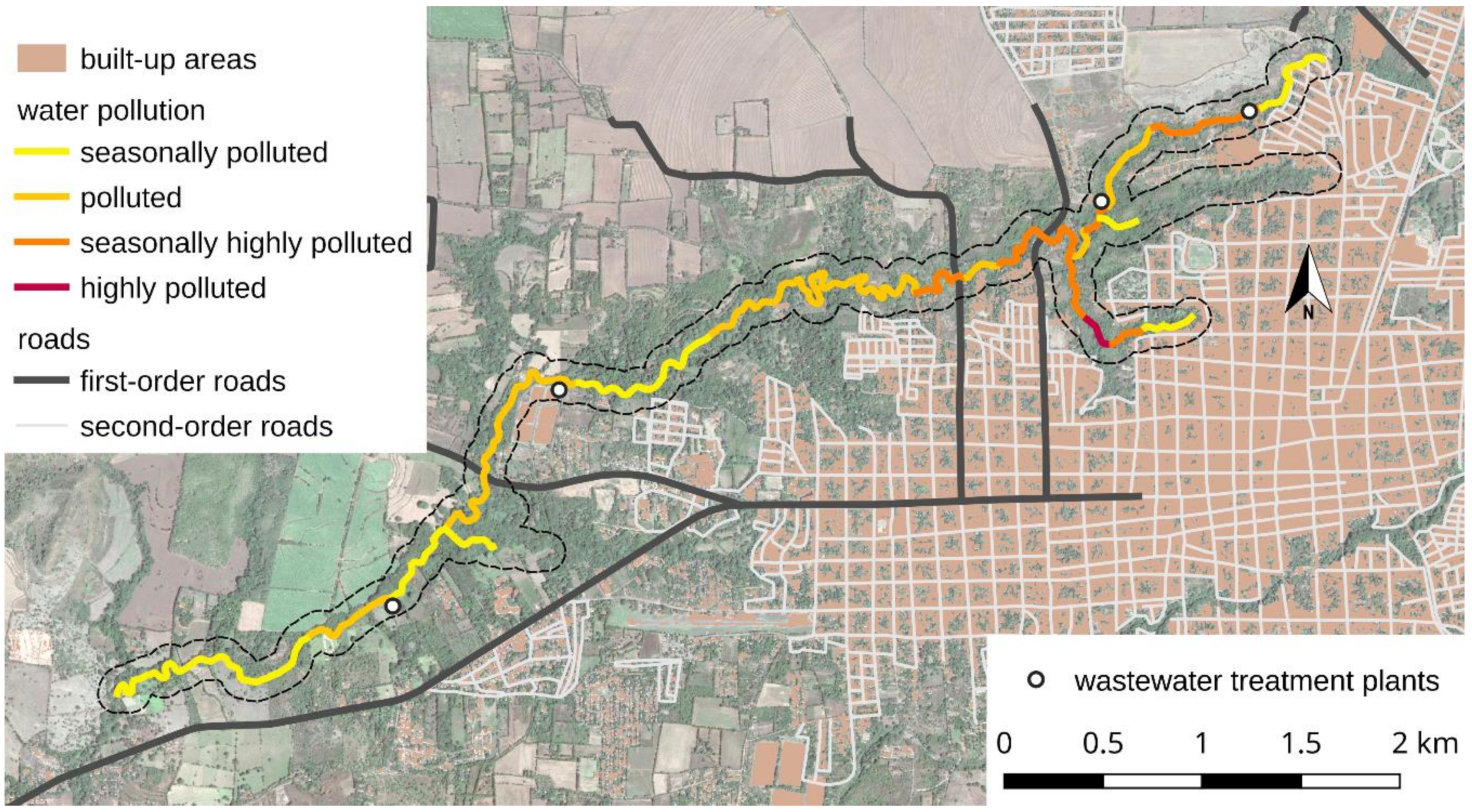
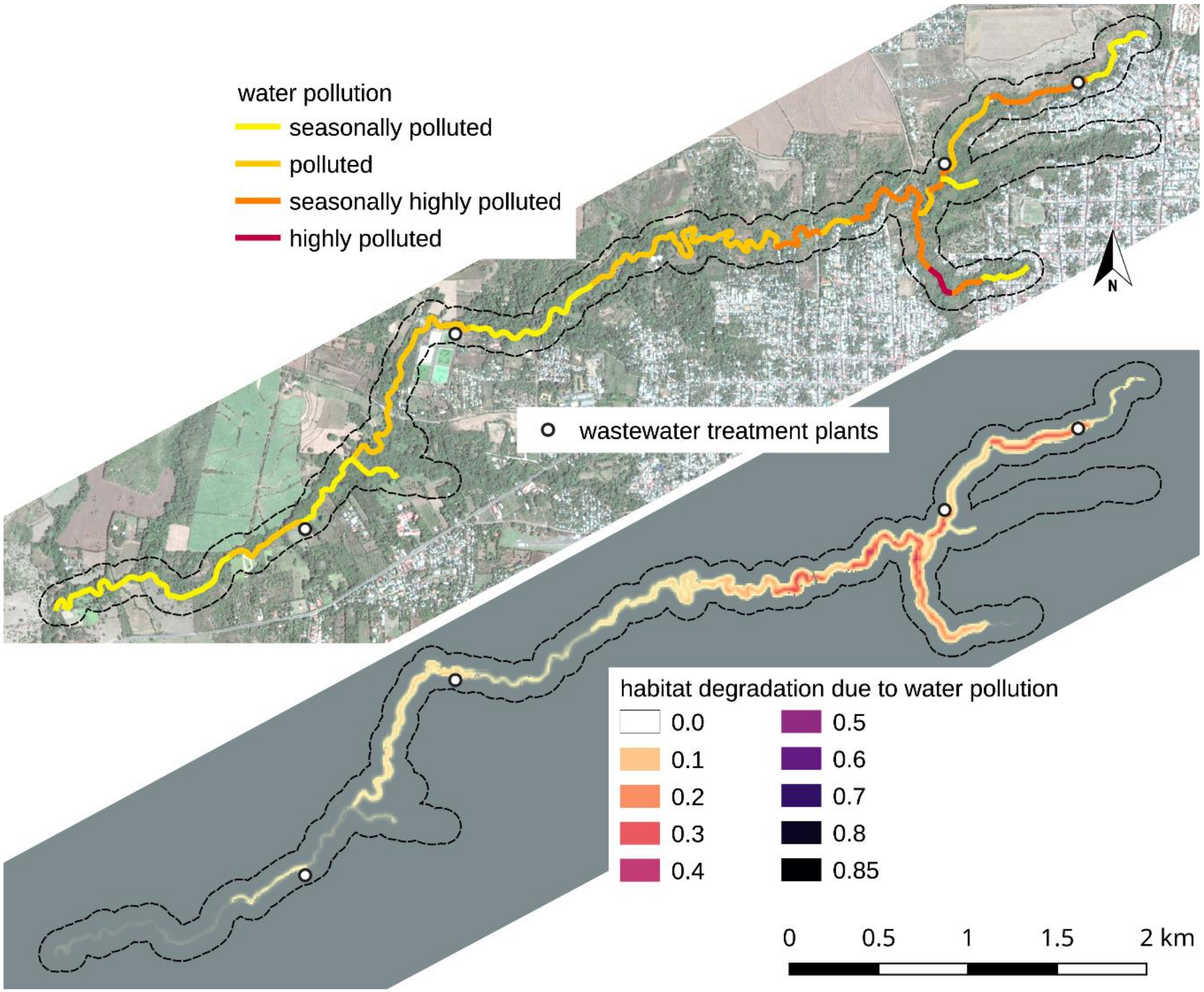
3.1.3. Habitat Degradation Due to Different Degrees of Water Pollution
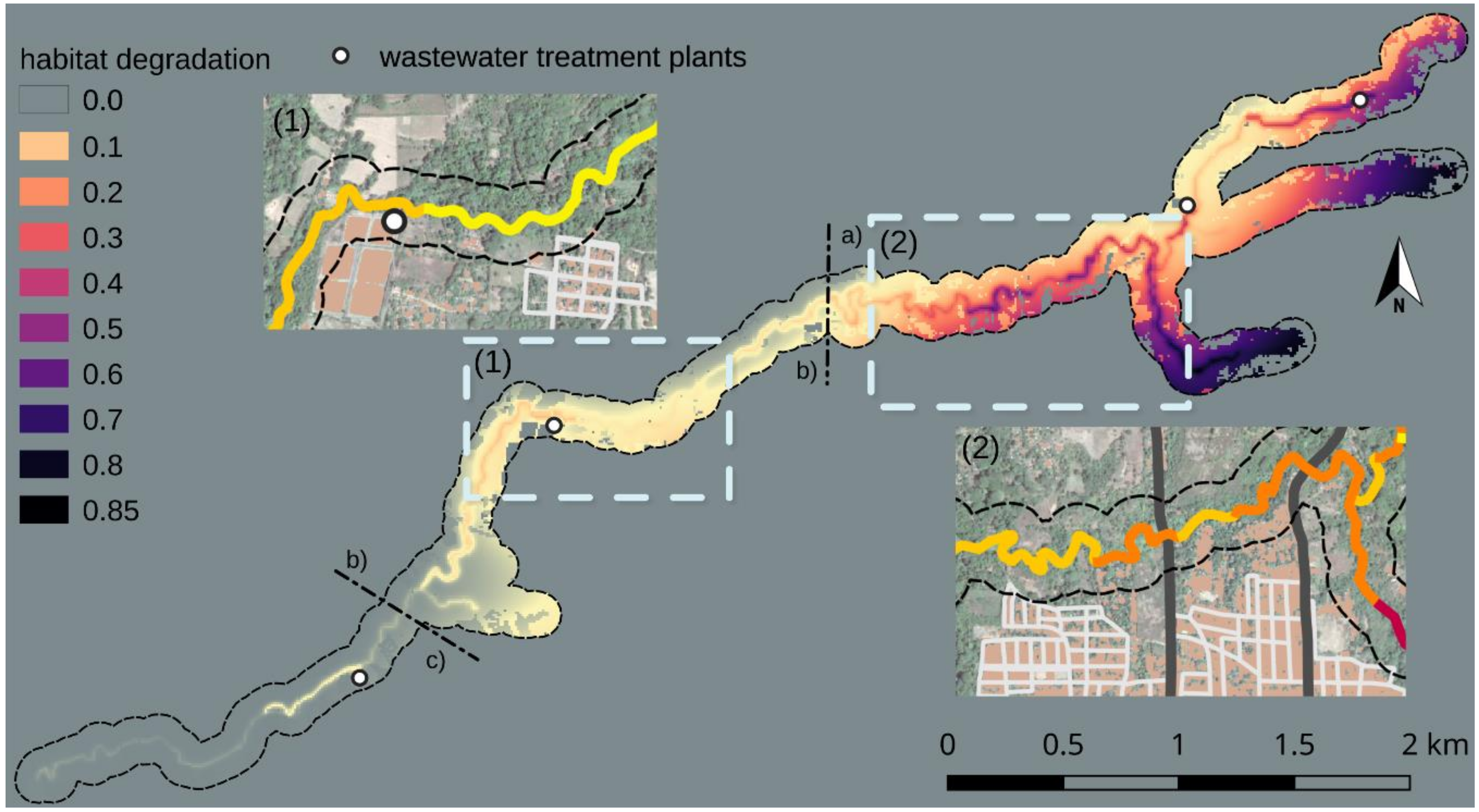
3.2. Habitat Degradation Due to the Combination of All Threats
3.3. Habitat Quality
4. Discussion
4.1. The Consideration of Additional LULC Classes for More Detailed Habitat Suitability Inputs
4.2. The Consideration of Additional LULC Class or Other Data Sources as Threats
4.3. Critical Reflection on the Model Parametrization and Model Limitations
4.4. Suggestions for Improvements and Further Studies
5. Conclusions
Author Contributions
Funding
Acknowledgments
Conflicts of Interest
References
- Díazo, S.; Settele, J.; Brondízio, E.; Ngo, H.T.; Guèze, M.; Agard, J.; Arneth, A.; Balvanera, P.; Brauman, K.; Butchart, S.; et al. Summary for Policymakers of the Global Assessment Report on Biodiversity and Ecosystem Services; Intergovernmental Science-Policy Platform on Biodiversity and Ecosystem Services (IPBES): Paris, France, 2019. [Google Scholar]
- IPBES. Global Assessment Report on Biodiversity and Ecosystem Services; IPBES: Paris, France, 2019. [Google Scholar]
- Walsh, C.J.; Booth, D.B.; Burns, M.J.; Fletcher, T.D.; Hale, R.L.; Hoang, L.N.; Livingston, G.; Rippy, M.A.; Roy, A.H.; Scoggins, M.; et al. Principles for urban stormwater management to protect stream ecosystems. Freshw. Sci. 2016, 35, 398–411. [Google Scholar] [CrossRef] [Green Version]
- Beißler, M.R.; Hack, J. A Combined Field and Remote-Sensing based Methodology to Assess the Ecosystem Service Potential of Urban Rivers in Developing Countries. Remote Sens. 2019, 11, 1697. [Google Scholar] [CrossRef] [Green Version]
- Dietrich, A.; Yarlagadda, R.; Gruden, C. Estimating the potential benefits of green stormwater infrastructure on developed sites using hydrologic model simulation. Environ. Prog. Sustain. Energy 2017, 36, 557–564. [Google Scholar] [CrossRef]
- Gustafson, E.J. Minireview: Quantifying Landscape Spatial Pattern: What Is the State of the Art? Ecosystems 1998, 1, 143–156. [Google Scholar] [CrossRef]
- Guisan, A.; Zimmermann, N.E. Predictive habitat distribution models in ecology. Ecol. Model. 2000, 135, 147–186. [Google Scholar] [CrossRef]
- Di Febbraro, M.; Sallustio, L.; Vizzarri, M.; De Rosa, D.; De Lisio, L.; Loy, A.; Eichelberger, B.A.; Marchetti, M. Expert-based and correlative models to map habitat quality: Which gives better support to conservation planning? Glob. Ecol. Conserv. 2018, 16, e00513. [Google Scholar] [CrossRef]
- Duarte, G.T.; Ribeiro, M.C.; Paglia, A.P. Ecosystem Services Modeling as a Tool for Defining Priority Areas for Conservation. PLoS ONE 2016, 11, e0154573. [Google Scholar] [CrossRef] [Green Version]
- McShea, W.J. What are the roles of species distribution models in conservation planning? Environ. Conserv. 2014, 41, 93–96. [Google Scholar] [CrossRef] [Green Version]
- Sharp, R.; Tallis, H.T.; Ricketts, T.; Guerry, A.D.; Wood, S.A.; Chaplin-Kramer, R.; Nelson, E.; Ennaanay, D.; Wolny, S.; Olwero, N.; et al. InVEST 3.4.4. User’s Guide 2018; Natural Capital Project: Standford, CA, USA, 2018. [Google Scholar]
- Bhagabati, N.K.; Ricketts, T.; Sulistyawan, T.B.S.; Conte, M.; Ennaanay, D.; Hadian, O.; McKenzie, E.; Olwero, N.; Rosenthal, A.; Tallis, H.; et al. Ecosystem services reinforce Sumatran tiger conservation in land use plans. Biol. Conserv. 2014, 169, 147–156. [Google Scholar] [CrossRef]
- Sharma, R.; Rimal, B.; Stork, N.; Baral, H.; Dhakal, M. Spatial Assessment of the Potential Impact of Infrastructure Development on Biodiversity Conservation in Lowland Nepal. ISPRS Int. J. Geo Inform. 2018, 7, 365. [Google Scholar] [CrossRef] [Green Version]
- Terrado, M.; Sabater, S.; Chaplin-Kramer, B.; Mandle, L.; Ziv, G.; Acuña, V. Model development for the assessment of terrestrial and aquatic habitat quality in conservation planning. Sci. Total Environ. 2016, 540, 63–70. [Google Scholar] [CrossRef] [Green Version]
- Alcaldía Municipal de León Datos Generales del Municipio León. Available online: http://www.leonmunicipio.com/uploads/1/3/8/2/1382165/datos_generales_del_municipio_de_len.pdf (accessed on 9 November 2019).
- Lüke, A.; Hack, J. Comparing the Applicability of Commonly Used Hydrological Ecosystem Services Models for Integrated Decision-Support. Sustainability 2018, 10, 346. [Google Scholar] [CrossRef] [Green Version]
- Bach, A.; Kipp, C. Photo Documentation of the Río Pochote—Geocoding of the Course of the River with GPS and Localisation of Freshwater Springs, Sewage Discharges and Specific Characteristics; Technical University Darmstadt: León, Nicaragua, 2017. [Google Scholar]
- Natural Capital Project Habitat Quality; Stanford University: Stanford, CA, USA, 2017.
- World Wide Fund for Nature. The Natural Capital Project. Available online: https://www.worldwildlife.org/projects/the-natural-capital-project (accessed on 23 April 2020).
- Hall, L.S.; Krausman, P.R.; Morrison, M.L. The habitat concept and a plea for standard terminology. Wildl. Soc. Bull. 1997, 25, 173–182. [Google Scholar]
- Kareiva, P.M. Natural Capital; Kareiva, P., Tallis, H., Ricketts, T.H., Daily, G.C., Polasky, S., Eds.; Oxford University Press: New York, NY, USA, 2011; ISBN 9780199588992. [Google Scholar]
- Forman, R.T.T.; Sperling, D.; Bissonette, J.A.; Clevenger, A.P.; Cutshall, C.D.; Dale, V.H.; Fahrig, L.; France, R.L.; Heanue, K.; Goldman, C.R. Road Ecology: Science and Solutions; Island Press: Washington, DC, USA, 2003. [Google Scholar]
- Nellemann, C.; Kullerud, L.; Vistnes, I.; Forbes, B.C.; Husby, E.; Kofinas, G.P.; Kaltenborn, B.P.; Rouaud, J.; Magomedova, M.; Bobiwash, R.; et al. GLOBIO. Global Methodology for Mapping Human Impacts on the Biosphere; UNEP-DEWA: Nairobi, Kenya, 2001. [Google Scholar]
- McKinney, M. Urbanization, Biodiversity, and Conservation: The impacts of urbanization on native species are poorly studied, but educating a highly urbanized human population about these impacts can greatly improve species conservation in all ecosystems. Bioscience 2002, 52, 883–890. [Google Scholar] [CrossRef]
- Johnson, M.D. Habitat quality: A brief review for wildlife biologists. Trans. West. Sect. Wildl. Soc. 2005, 2005, 31–43. [Google Scholar]
- QGIS Development Team. QGIS User Guide—Release 2.18. 2019. Available online: https://docs.qgis.org/2.18/en/docs/user_manual/ (accessed on 22 April 2020).
- Seiler, A. Ecological Effects of Roads—A review; Swedish University of Agricultural Sciences: Uppsala, Sweden, 2001. [Google Scholar]
- Rimal, B.; Sharma, R.; Kunwar, R.; Keshtkar, H.; Stork, N.E.; Rijal, S.; Rahman, S.A.; Baral, H. Effects of land use and land cover change on ecosystem services in the Koshi River Basin, Eastern Nepal. Ecosyst. Serv. 2019, 38, 100963. [Google Scholar] [CrossRef]
- Wu, Y.; Tao, Y.; Yang, G.; Ou, W.; Pueppke, S.; Sun, X.; Chen, G.; Tao, Q. Impact of land use change on multiple ecosystem services in the rapidly urbanizing Kunshan City of China: Past trajectories and future projections. Land Use Policy 2019, 85, 419–427. [Google Scholar] [CrossRef]
- Sun, X.; Jiang, Z.; Liu, F.; Zhang, D. Monitoring spatio-temporal dynamics of habitat quality in Nansihu Lake basin, eastern China, from 1980 to 2015. Ecol. Indic. 2019, 102, 716–723. [Google Scholar] [CrossRef]
- Baral, H.; Keenan, R.J.; Sharma, S.K.; Stork, N.E.; Kasel, S. Spatial assessment and mapping of biodiversity and conservation priorities in a heavily modified and fragmented production landscape in north-central Victoria, Australia. Ecol. Indic. 2014, 36, 552–562. [Google Scholar] [CrossRef]
- Sun, X.; Lu, Z.; Li, F.; Crittenden, J.C. Analyzing spatio-temporal changes and trade-offs to support the supply of multiple ecosystem services in Beijing, China. Ecol. Indic. 2018, 94, 117–129. [Google Scholar] [CrossRef]
- Deng, J.; Lin, Y.; Zhou, M.; Wu, C.; Chen, B.; Xiao, G.; Cai, J. Ecosystem services dynamics response to tremendous reclamation in a coastal island city. Ecosyst. Heal. Sustain. 2019, 1–14. [Google Scholar] [CrossRef] [Green Version]
- Cao, W.; Li, R.; Chi, X.; Chen, N.; Chen, J.; Zhang, H.; Zhang, F. Island urbanization and its ecological consequences: A case study in the Zhoushan Island, East China. Ecol. Indic. 2017, 76, 1–14. [Google Scholar] [CrossRef]
- Han, Y.; Kang, W.; Thorne, J.; Song, Y. Modeling the effects of landscape patterns of current forests on the habitat quality of historical remnants in a highly urbanized area. Urban For. Urban Green. 2019, 41, 354–363. [Google Scholar] [CrossRef]
- Xu, Q.; Zheng, X.; Zheng, M. Do urban planning policies meet sustainable urbanization goals? A scenario-based study in Beijing, China. Sci. Total Environ. 2019, 670, 498–507. [Google Scholar] [CrossRef]
- Xu, L.; Chen, S.S.; Xu, Y.; Li, G.; Su, W. Impacts of land-use change on habitat quality during 1985–2015 in the Taihu Lake Basin. Sustainability 2019, 11, 3513. [Google Scholar] [CrossRef] [Green Version]
- Medley, K.E.; McDonnell, M.J.; Pickett, S. Forest-landscape structure along an urban-to-rural gradient. Prof. Geogr. 1995, 47, 159–168. [Google Scholar] [CrossRef]
- Sukopp, H.; Werner, P. Nature in Cities; Council of Europe: Strasbourg, France, 1982. [Google Scholar]
- Pickett, S.T.A.; Cadenasso, M.L.; Grove, J.M.; Nilon, C.H.; Pouyat, R.V.; Zipperer, W.C.; Costanza, R. Urban Ecological Systems: Linking Terrestrial Ecological, Physical, and Socioeconomic Components of Metropolitan Areas. In Urban Ecology; Springer US: Boston, MA, USA, 2001; pp. 99–122. [Google Scholar]
- Gong, J.; Xie, Y.; Cao, E.; Huang, Q.; Li, H. Integration of InVEST-habitat quality model with landscape pattern indexes to assess mountain plant biodiversity change: A case study of Bailongjiang watershed in Gansu Province. J. Geogr. Sci. 2019, 29, 1193–1210. [Google Scholar] [CrossRef] [Green Version]
- Sulistyawan, B.S.; Eichelberger, B.A.; Verweij, P.; Boot, R.G.A.; Hardian, O.; Adzan, G.; Sukmantoro, W. Connecting the fragmented habitat of endangered mammals in the landscape of Riau–Jambi–Sumatera Barat (RIMBA), central Sumatra, Indonesia (connecting the fragmented habitat due to road development). Glob. Ecol. Conserv. 2017, 9, 116–130. [Google Scholar] [CrossRef]
- Lin, Y.-P.; Lin, W.-C.; Wang, Y.-C.; Lien, W.-Y.; Huang, T.; Hsu, C.-C.; Schmeller, D.S.; Crossman, N.D. Systematically designating conservation areas for protecting habitat quality and multiple ecosystem services. Environ. Model. Softw. 2017, 90, 126–146. [Google Scholar] [CrossRef]
- Natural Capital Project in Development: Urban InVEST. Available online: https://naturalcapitalproject.stanford.edu/software/invest-models/development-urban-invest (accessed on 6 February 2020).


| Land Cover | Description |
|---|---|
| High vegetation | Unmanaged land dominated by trees |
| Low vegetation | Managed land with bushes, grassland, and degraded forests |
| Built-up area | Buildings of all kinds (mainly residential houses) considered as non-habitats for wildlife |
| Threats | Max. Effective Distance (km) | Weight (–) | Decay over Space | LULC Classes | ||
|---|---|---|---|---|---|---|
| High Vegetation | Low Vegetation | Built-Up Area | ||||
| Habitat Suitability Score (–) | ||||||
| 1 | 0.6 | 0 | ||||
| Sensitivity Score of Habitats to Threats (–) | ||||||
| Built-up area | 0.2 | 1 | exp. | 0.8 | 0.7 | 0 |
| First-order road | 0.2 | 0.8 | exp. | 0.8 | 0.7 | 0 |
| Second-order road | 0.2 | 0.7 | exp. | 0.6 | 0.5 | 0 |
| Water pollution—seasonally polluted | 0.01 | 0.1 | exp. | 0.6 | 0.4 | 0 |
| Water pollution—polluted | 0.01 | 0.3 | exp. | 0.6 | 0.4 | 0 |
| Water pollution—seasonally highly polluted | 0.01 | 0.7 | exp. | 0.6 | 0.4 | 0 |
| Water pollution—highly polluted | 0.01 | 0.9 | exp. | 0.6 | 0.4 | 0 |
© 2020 by the authors. Licensee MDPI, Basel, Switzerland. This article is an open access article distributed under the terms and conditions of the Creative Commons Attribution (CC BY) license (http://creativecommons.org/licenses/by/4.0/).
Share and Cite
Hack, J.; Molewijk, D.; Beißler, M.R. A Conceptual Approach to Modeling the Geospatial Impact of Typical Urban Threats on the Habitat Quality of River Corridors. Remote Sens. 2020, 12, 1345. https://0-doi-org.brum.beds.ac.uk/10.3390/rs12081345
Hack J, Molewijk D, Beißler MR. A Conceptual Approach to Modeling the Geospatial Impact of Typical Urban Threats on the Habitat Quality of River Corridors. Remote Sensing. 2020; 12(8):1345. https://0-doi-org.brum.beds.ac.uk/10.3390/rs12081345
Chicago/Turabian StyleHack, Jochen, Diana Molewijk, and Manuel R. Beißler. 2020. "A Conceptual Approach to Modeling the Geospatial Impact of Typical Urban Threats on the Habitat Quality of River Corridors" Remote Sensing 12, no. 8: 1345. https://0-doi-org.brum.beds.ac.uk/10.3390/rs12081345