Evolution of Backscattering Coefficients of Drifting Multi-Year Sea Ice during End of Melting and Onset of Freeze-up in the Western Beaufort Sea

 ,
,  , , ,
, , ,  , ,
, ,
Abstract
:
1. Introduction
2. Materials and Methods
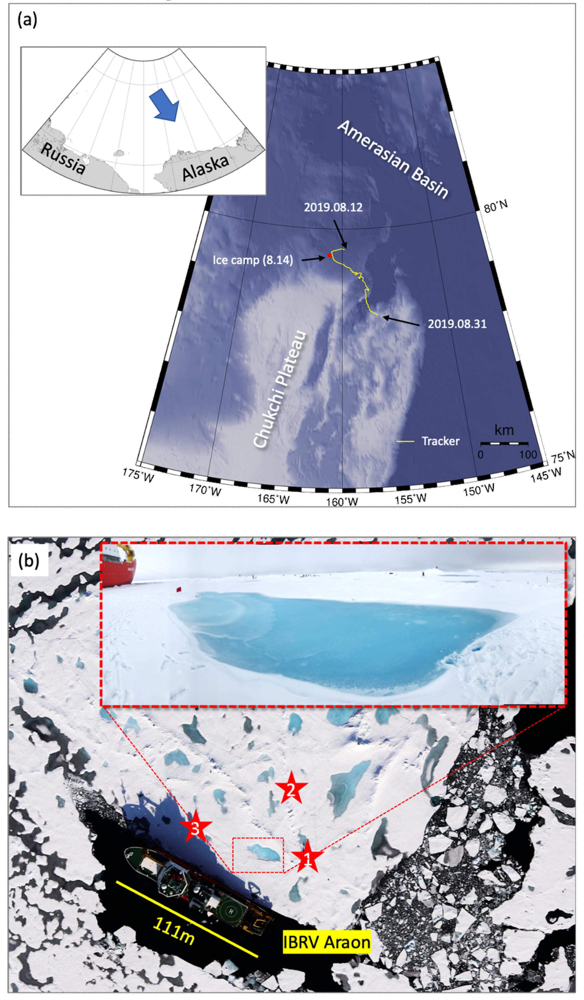
2.1. Study Area
2.2. Methods
2.2.1. Installation of a GPS Tracker on a Sea Ice Floe
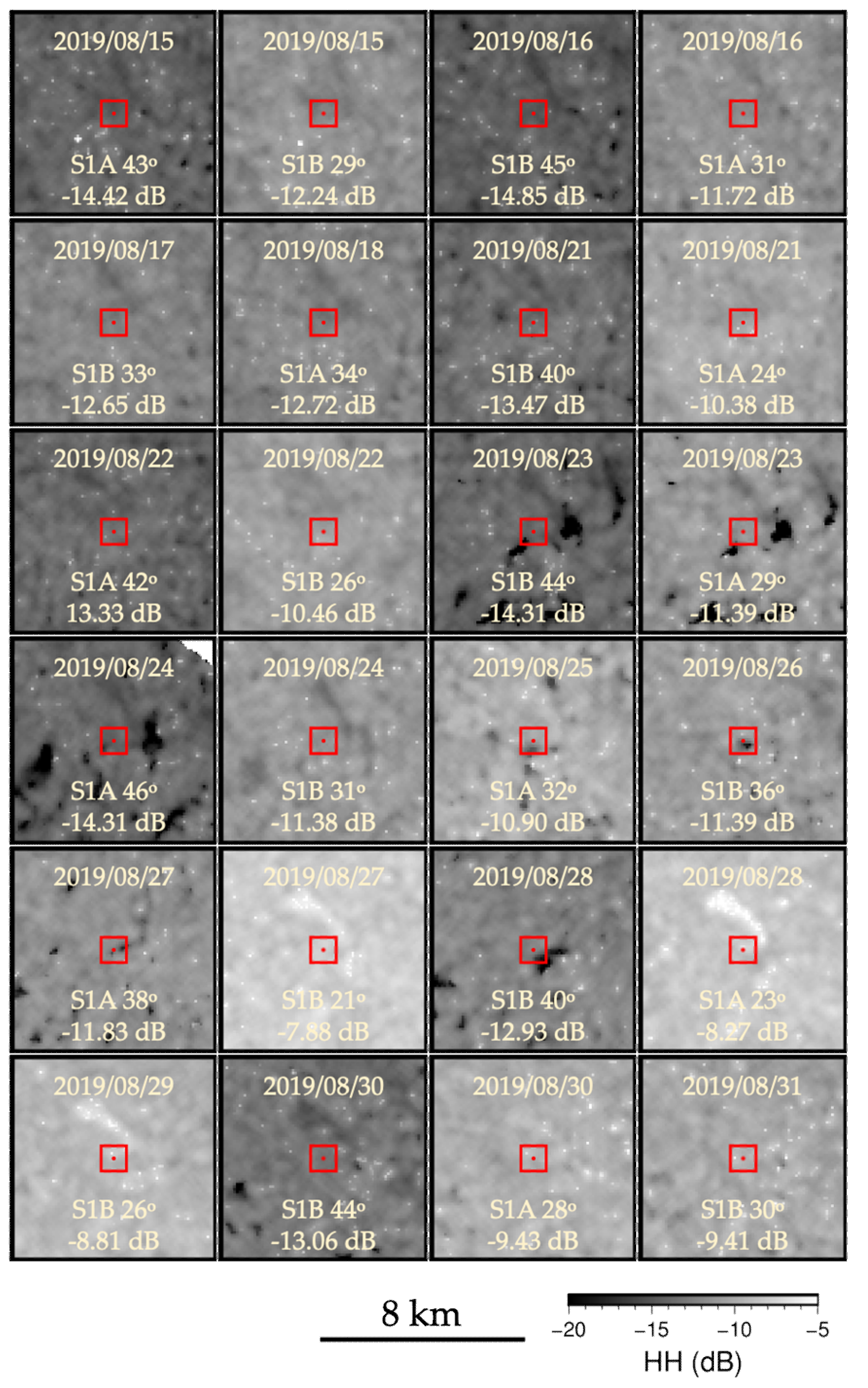
2.2.2. Processing of Sentinel-1 C-Band SAR Data
2.2.3. Calculation of the Incidence Angle Dependence and Temporal Analysis of the Normalized Backscattering Coefficients
2.2.4. Atmospheric Effects on the Backscattering Coefficients
3. Results
4. Discussion
5. Conclusions
Author Contributions
Funding
Acknowledgments
Conflicts of Interest
References
- Curry, J.A.; Schramm, J.L.; Ebert, E.E. Sea Ice-Albedo Climate Feedback Mechanism. J. Clim. 1995, 8, 240–247. [Google Scholar] [CrossRef]
- McBean, G.; Alekseev, G.; Chen, D.; Førland, E.; Fyfe, J.; Groisman, P.; King, R.; Melling, H.; Vose, R.; Whitfield, P. Arctic Climate—Past and Present. Arctic Climate Impact Assessment: Scientific Report; Cambridge University Press: Cambridge, UK, 2005; pp. 22–60. [Google Scholar]
- Serreze, M.C.; Holland, M.M.; Stroeve, J. Perspectives on the Arctic’s Shrinking Sea-Ice Cover. Science 2007, 315, 1533–1536. [Google Scholar] [CrossRef] [PubMed] [Green Version]
- Stroeve, J.C.; Holland, M.M.; Meier, W.; Scambos, T.; Serreze, M. Arctic sea ice decline: Faster than forecast. Geophys. Res. Lett. 2007, 34. [Google Scholar] [CrossRef]
- Kwok, R. Arctic sea ice thickness, volume, and multiyear ice coverage: Losses and coupled variability (1958–2018). Environ. Res. Lett. 2018, 13. [Google Scholar] [CrossRef]
- Budikova, D. Role of Arctic sea ice in global atmospheric circulation: A review. Glob. Planet Chang. 2009, 68, 149–163. [Google Scholar] [CrossRef]
- Stroeve, J.C.; Serreze, M.C.; Holland, M.M.; Kay, J.E.; Malanik, J.; Barrett, A.P. The Arctic’s rapidly shrinking sea ice cover: A research synthesis. Clim. Chang. 2012, 110, 1005–1027. [Google Scholar] [CrossRef] [Green Version]
- Kwok, R. Sea ice convergence along the Arctic coasts of Greenland and the Canadian Arctic Archipelago: Variability and extremes (1992–2014). Geophys. Res. Lett. 2015, 42, 7598–7605. [Google Scholar] [CrossRef]
- Galley, R.J.; Babb, D.; Ogi, M.; Else, B.; Geilfus, N.X.; Crabeck, O.; Barber, D.G.; Rysgaard, S. Replacement of multiyear sea ice and changes in the open water season duration in the Beaufort Sea since 2004. J. Geophys. Res. 2016, 121, 1806–1823. [Google Scholar] [CrossRef] [Green Version]
- Zakhvatkina, N.Y.; Alexandrov, V.Y.; Johannessen, O.M.; Sandven, S.; Frolov, I.Y. Classification of Sea Ice Types in ENVISAT Synthetic Aperture Radar Images. IEEE Trans. Geosci. Remote 2013, 51, 2587–2600. [Google Scholar] [CrossRef]
- Han, H.; Hong, S.H.; Kim, H.C.; Chae, T.B.; Choi, H.J. A study of the feasibility of using KOMPSAT-5 SAR data to map sea ice in the Chukchi Sea in late summer. Remote Sens. Lett. 2017, 8, 468–477. [Google Scholar] [CrossRef]
- Karvonen, J.; Simila, M.; Mäkynen, M. Open water detection from Baltic Sea ice Radarsat-1 SAR imagery. IEEE Geosci. Remote 2005, 2, 275–279. [Google Scholar] [CrossRef]
- Karvonen, J. Evaluation of the operational SAR based Baltic Sea ice concentration products. Adv. Space Res. 2015, 56, 119–132. [Google Scholar] [CrossRef]
- Dierking, W.; Dall, J. Sea-Ice Deformation State from Synthetic Aperture Radar Imagery—Part I: Comparison of C-and L-Band and Different Polarization. IEEE Trans. Geosci. Remote. 2007, 45, 3610–3622. [Google Scholar] [CrossRef]
- Casey, J.A.; Howell, S.E.; Tivy, A.; Haas, C. Separability of sea ice types from wide swath C-and L-band synthetic aperture radar imagery acquired during the melt season. Remote Sens. Environ. 2016, 174, 314–328. [Google Scholar] [CrossRef] [Green Version]
- Geldsetzer, T.; Yackel, J. Sea ice type and open water discrimination using dual co-polarized C-band SAR. Can. J. Remote Sens. 2009, 35, 73–84. [Google Scholar] [CrossRef]
- Geldsetzer, T.; Arkett, M.; Zagon, T.; Charbonneau, F.; Yackel, J.J.; Scharien, R.K. All-Season Compact-Polarimetry C-band SAR Observations of Sea Ice. Can. J. Remote Sens. 2015, 41, 485–504. [Google Scholar] [CrossRef]
- Mäkynen, M.P.; Manninen, A.T.; Simila, M.H.; Karvonen, J.A.; Hallikainen, M.T. Incidence angle dependence of the statistical properties of C-band HH-polarization backscattering signatures of the Baltic Sea ice. IEEE T. Geosci. Remote 2002, 40, 2593–2605. [Google Scholar] [CrossRef]
- Mäkynen, M.; Kern, S.; Rosel, A.; Pedersen, L.T. On the Estimation of Melt Pond Fraction on the Arctic Sea Ice With ENVISAT WSM Images. IEEE T. Geosci. Remote 2014, 52, 7366–7379. [Google Scholar] [CrossRef]
- Onstott, R.G. SAR and Scatterometer Signatures of Sea Ice. In Microwave Remote Sensing of Sea Ice; Carsey, F., Ed.; American Geophysical Union: Washington, DC, USA, 1992; Volume 68, pp. 73–104. [Google Scholar] [CrossRef]
- Mahmud, M.S.; Geldsetzer, T.; Howell, S.E.L.; Yackel, J.J.; Nandan, V.; Scharien, R.K. Incidence Angle Dependence of HH-Polarized C- and L-Band Wintertime Backscatter Over Arctic Sea Ice. IEEE T. Geosci. Remote 2018, 56, 6686–6698. [Google Scholar] [CrossRef]
- Lubin, D.; Massom, R. Polar Remote Sensing: Volume I: Atmosphere and Oceans; Springer Science & Business Media: Berlin, Germany, 2006; p. 320. [Google Scholar]
- McPhee, M.G.; Maykut, G.A.; Morison, J.H. Dynamics and Thermodynamics of the Ice Upper Ocean System in the Marginal Ice-Zone of the Greenland Sea. J. Geophys. Res. Oceans 1987, 92, 7017–7031. [Google Scholar] [CrossRef]
- Winebrenner, D.P.; Holt, B.; Nelson, E.D. Observation of autumn freeze-up in the Beaufort and Chukchi Seas using the ERS 1 synthetic aperture radar. J. Geophys. Res. Oceans 1996, 101, 16401–16419. [Google Scholar] [CrossRef]
- Dierking, W. Mapping of Different Sea Ice Regimes Using Images From Sentinel-1 and ALOS Synthetic Aperture Radar. IEEE Trans. Geosci. Remote 2010, 48, 1045–1058. [Google Scholar] [CrossRef]
- Thoman, R.L.; Bhatt, U.S.; Bieniek, P.A.; Brettschneider, B.R.; Brubaker, M.; Danielson, S.L.; Labe, Z.; Lader, R.; Meier, W.N.; Sheffield, G. The Record Low Bering Sea Ice Extent in 2018: Context, Impacts, and an Assessment of the Role of Anthropogenic Climate Change. Am. Meteorol. Soc. 2020, 101, S53–S58. [Google Scholar] [CrossRef] [Green Version]
- Holt, B.; Digby, S.A. Processes and imagery of first-year fast sea ice during the melt season. J. Geophys. Res. Oceans 1985, 90, 5045–5062. [Google Scholar] [CrossRef]
- Barber, D.G.; Yackel, J. The physical, radiative and microwave scattering characteristics of melt ponds on Arctic landfast sea ice. Int. J. Remote Sens. 1999, 20, 2069–2090. [Google Scholar] [CrossRef]
- Torres, R.; Snoeij, P.; Geudtner, D.; Bibby, D.; Davidson, M.; Attema, E.; Potin, P.; Rommen, B.; Floury, N.; Brown, M. GMES Sentinel-1 mission. Remote Sens. Environ. 2012, 120, 9–24. [Google Scholar] [CrossRef]
- Mäkynen, M.; Karvonen, J. Incidence Angle Dependence of First-Year Sea Ice Backscattering Coefficient in Sentinel-1 SAR Imagery Over the Kara Sea. IEEE T. Geosci. Remote 2017, 55, 6170–6181. [Google Scholar] [CrossRef]
- Hersbach, H.; Bell, B.; Berrisford, P.; Horányi, A.; Sabater, J.M.; Nicolas, J.; Radu, R.; Schepers, D.; Simmons, A.; Soci, C. Global reanalysis: Goodbye ERA-Interim, hello ERA5. ECMWF Newsl. 2019, 159, 17–24. [Google Scholar]
- Onstott, R.G.; Grenfell, T.C.; Matzler, C.; Luther, C.A.; Svendsen, E.A. Evolution of Microwave Sea Ice Signatures during Early Summer and Midsummer in the Marginal Ice-Zone. J. Geophys. Res. 1987, 92, 6825–6835. [Google Scholar] [CrossRef]
- Ulander, L.; Carlström, A. Radar backscatter signatures of Baltic sea ice. In Proceedings of the IGARSS’91 Remote Sensing: Global Monitoring for Earth Management, Espoo, Finland, 3–6 June 1991; Volume 3, pp. 1215–1218. [Google Scholar] [CrossRef]
- Nandan, V.; Geldsetzer, T.; Mahmud, M.; Yackel, J.; Ramjan, S. Ku-, X-and C-Band Microwave Backscatter Indices from Saline Snow Covers on Arctic First-Year Sea Ice. Remote Sens. 2017, 9. [Google Scholar] [CrossRef] [Green Version]
- Jeffries, M.; Schwartz, K.; Li, S. Arctic summer sea-ice SAR signatures, melt-season characteristics, and melt-pond fractions. Polar Rec. 1997, 33, 101–112. [Google Scholar] [CrossRef]
- Geldsetzer, T.; Mead, J.B.; Yackel, J.J.; Scharien, R.K.; Howell, S.E. Surface-based polarimetric C-band scatterometer for field measurements of sea ice. IEEE Trans. Geosci. Remote 2007, 45, 3405–3416. [Google Scholar] [CrossRef]
- Carlström, A.; Ulander, L.M. C-band backscatter signatures of old sea ice in the central Arctic during freeze-up. IEEE Trans. Geosci. Remote 1993, 31, 819–829. [Google Scholar] [CrossRef]
- Zhou, X.; Chong, J.; Bi, H.; Yu, X.; Shi, Y.; Ye, X. Directional Spreading Function of the Gravity-Capillary Wave Spectrum Derived from Radar Observations. Remote Sens. 2017, 9, 361. [Google Scholar] [CrossRef] [Green Version]
- Yang, J.; Comiso, J.; Walsh, D.; Krishfield, R.; Honjo, S. Storm-driven mixing and potential impact on the Arctic Ocean. J. Geophys. Res. Oceans 2004, 109. [Google Scholar] [CrossRef]
- Graham, R.M.; Itkin, P.; Meyer, A.; Sundfjord, A.; Spreen, G.; Smedsrud, L.H.; Liston, G.E.; Cheng, B.; Cohen, L.; Divine, D. Winter storms accelerate the demise of sea ice in the Atlantic sector of the Arctic Ocean. Sci. Rep. 2019, 9, 9222. [Google Scholar] [CrossRef] [Green Version]
- Yackel, J.; Geldsetzer, T.; Mahmud, M.; Nandan, V.; Howell, S.E.; Scharien, R.K.; Lam, H.M. Snow Thickness Estimation on First-Year Sea Ice from Late Winter Spaceborne Scatterometer Backscatter Variance. Remote Sens. 2019, 11, 417. [Google Scholar] [CrossRef] [Green Version]
- Perovich, D.K.; Richter-Menge, J.A.; Jones, K.F.; Light, B. Sunlight, water, and ice: Extreme Arctic sea ice melt during the summer of 2007. Geophys. Res. Lett. 2008, 35. [Google Scholar] [CrossRef] [Green Version]
- Woodgate, R.A.; Weingartner, T.; Lindsay, R. The 2007 Bering Strait oceanic heat flux and anomalous Arctic sea-ice retreat. Geophys. Res. Lett. 2010, 37. [Google Scholar] [CrossRef] [Green Version]
- Perovich, D.K.; Richter-Menge, J.A.; Jones, K.F.; Light, B.; Elder, B.C.; Polashenski, C.; Laroche, D.; Markus, T.; Lindsay, R. Arctic sea-ice melt in 2008 and the role of solar heating. Ann. Glaciol. 2011, 52, 355–359. [Google Scholar] [CrossRef] [Green Version]
- Omstedt, A.; Wettlaufer, J. Ice growth and oceanic heat flux: Models and measurements. J. Geophys. Res. 1992, 97, 9383–9390. [Google Scholar] [CrossRef]
- Fetterer, F.; Knowles, K.; Meier, W.N.; Savoie, M.; Windnagel, A.K. Sea Ice Index, Version 3: Regional Daily Data; NSIDC: Boulder, CO, USA, 2017. [Google Scholar] [CrossRef]
- Timmermans, M.L.; Ladd, C. Arctic Report Card: Update for 2019. Available online: https://arctic.noaa.gov/Report-Card/Report-Card-2019/ArtMID/7916/ArticleID/840/Sea-Surface-Temperature (accessed on 2 January 2020).


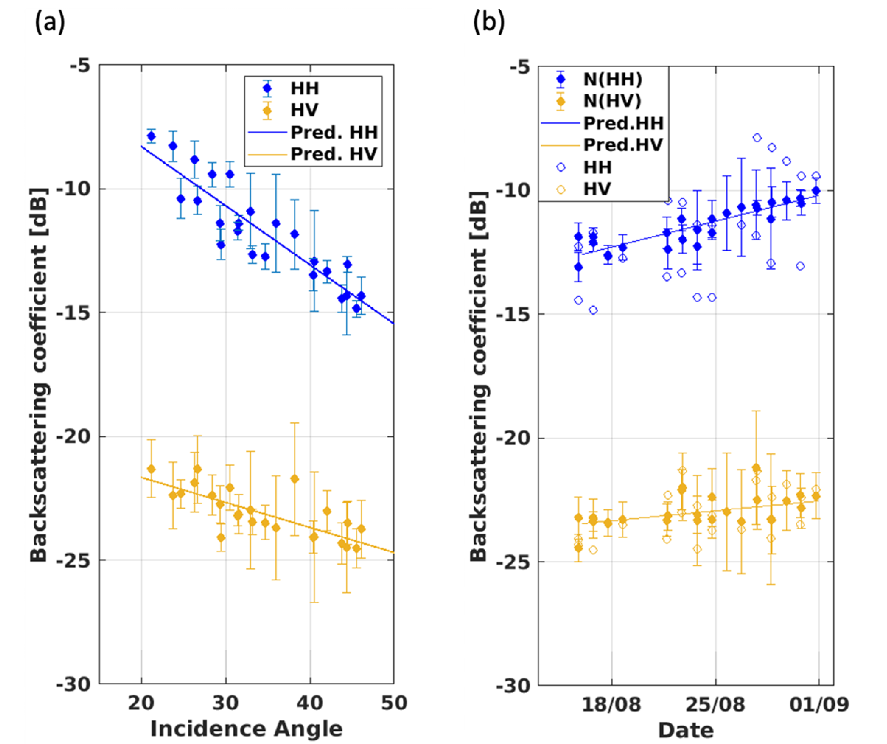
| Min [dB] | Max [dB] | Mean [dB] | |
|---|---|---|---|
| σ0HH | −14.85 | −7.89 | −11.73 ± 2.00 |
| N(σ0HH) | −13.10 | −10.01 | −11.39 ± 0.84 |
| σ0HV | −24.54 | −21.31 | −23.07 ± 0.98 |
| N(σ0HV) | −24.44 | −21.20 | −22.93 ± 0.67 |
| S(σ0HH) | 0.28 | 4.96 | 1.03 ± 0.92 |
| S(σ0HV) | 0.39 | 4.79 | 1.52 ± 0.78 |
| σ0HH | σ0HV | N(σ0HH) | N(σ0HV) | S(σ0HH) | S(σ0HV) | ||
|---|---|---|---|---|---|---|---|
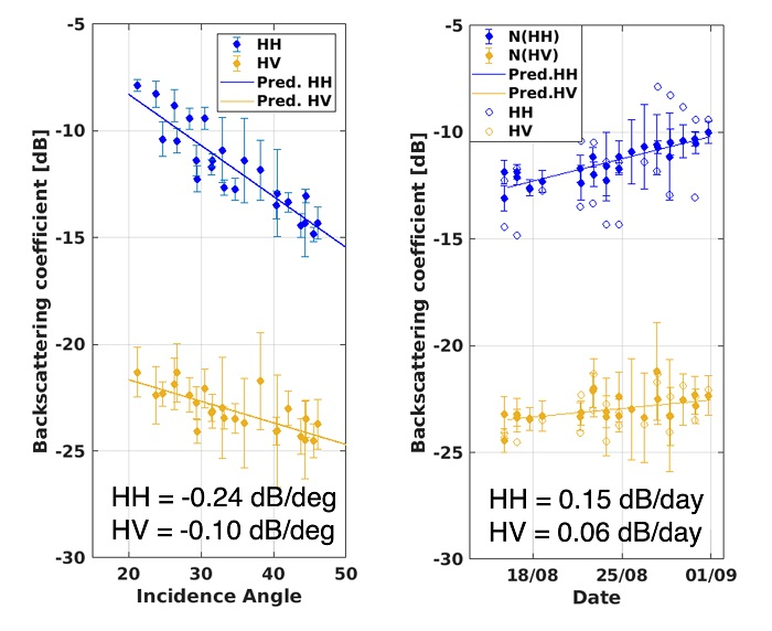
| Incidence Angle | Slope [dB/deg] | −0.24 | −0.10 | ||||
| R2 | 0.82 | 0.59 | |||||
| p-value | <0.01 | <0.01 | |||||
| Time | Slope [dB/day] | 0.22 | 0.10 | 0.15 | 0.06 | ||
| R2 | 0.28 | 0.25 | 0.76 | 0.24 | |||
| p-value | 0.008 | 0.012 | < 0.01 | 0.017 | |||
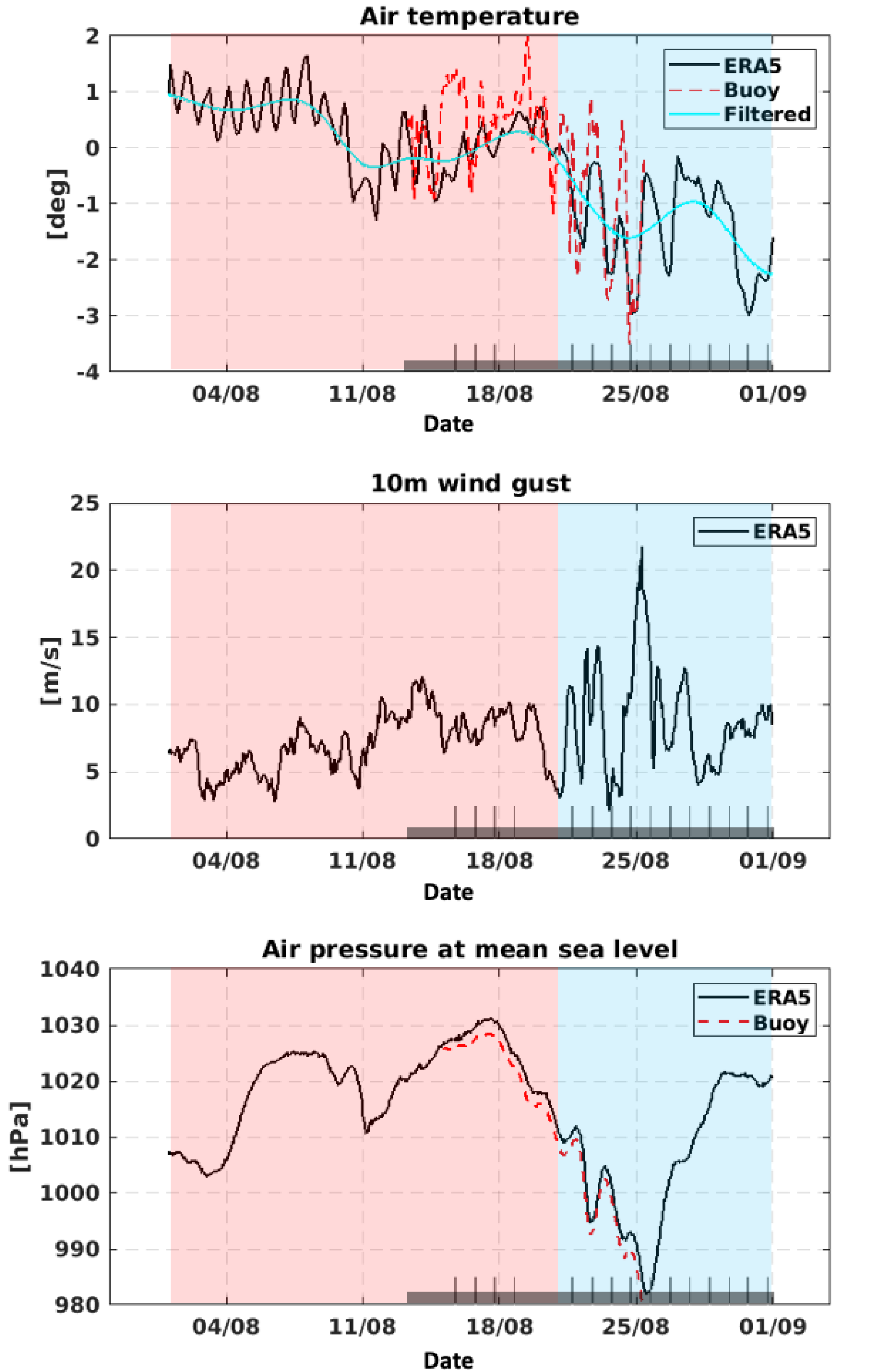
| Air temperature | ρ | −0.69 | −0.48 | −0.14 | −0.46 | ||
| p-value | < 0.01 | 0.018 | 0.502 | 0.026 | |||
| Wind gust | ρ | −0.07 | 0.37 | −0.16 | −0.12 | ||
| p-value | 0.728 | 0.079 | 0.456 | 0.567 | |||
| Pressure | ρ | −0.20 | −0.42 | −0.34 | −0.49 | ||
| p-value | 0.339 | 0.044 | 0.103 | 0.015 |
© 2020 by the authors. Licensee MDPI, Basel, Switzerland. This article is an open access article distributed under the terms and conditions of the Creative Commons Attribution (CC BY) license (http://creativecommons.org/licenses/by/4.0/).
Share and Cite
Kim, S.H.; Kim, H.-C.; Hyun, C.-U.; Lee, S.; Ha, J.-S.; Kim, J.-H.; Kwon, Y.-J.; Park, J.-W.; Han, H.; Jeong, S.-Y.; et al. Evolution of Backscattering Coefficients of Drifting Multi-Year Sea Ice during End of Melting and Onset of Freeze-up in the Western Beaufort Sea. Remote Sens. 2020, 12, 1378. https://0-doi-org.brum.beds.ac.uk/10.3390/rs12091378
Kim SH, Kim H-C, Hyun C-U, Lee S, Ha J-S, Kim J-H, Kwon Y-J, Park J-W, Han H, Jeong S-Y, et al. Evolution of Backscattering Coefficients of Drifting Multi-Year Sea Ice during End of Melting and Onset of Freeze-up in the Western Beaufort Sea. Remote Sensing. 2020; 12(9):1378. https://0-doi-org.brum.beds.ac.uk/10.3390/rs12091378
Chicago/Turabian StyleKim, Seung Hee, Hyun-Cheol Kim, Chang-Uk Hyun, Sungjae Lee, Jung-Seok Ha, Joo-Hong Kim, Young-Joo Kwon, Jeong-Won Park, Hyangsun Han, Seong-Yeob Jeong, and et al. 2020. "Evolution of Backscattering Coefficients of Drifting Multi-Year Sea Ice during End of Melting and Onset of Freeze-up in the Western Beaufort Sea" Remote Sensing 12, no. 9: 1378. https://0-doi-org.brum.beds.ac.uk/10.3390/rs12091378