HTD-Net: A Deep Convolutional Neural Network for Target Detection in Hyperspectral Imagery

1
College of Information Science and Technology, Beijing University of Chemical Technology, Beijing 100029, China
2
School of Information and Electronics, Beijing Institute of Technology, Beijing 100081, China
3
Department of Electrical and Computer Engineering, Mississippi State University, Starkville, MS 39762, USA
*
Author to whom correspondence should be addressed.
Remote Sens. 2020, 12(9), 1489; https://0-doi-org.brum.beds.ac.uk/10.3390/rs12091489
Submission received: 26 March 2020
/
Revised: 2 May 2020
/
Accepted: 3 May 2020
/
Published: 7 May 2020
(This article belongs to the Special Issue Advanced Techniques for Spaceborne Hyperspectral Remote Sensing)
Abstract
:In recent years, deep learning has dramatically improved the cognitive ability of the network by extracting depth features, and has been successfully applied in the field of feature extraction and classification of hyperspectral images. However, it is facing great difficulties for target detection due to extremely limited available labeled samples that are insufficient to train deep networks. In this paper, a novel target detection framework for deep learning is proposed, denoted as HTD-Net. To overcome the few-training-sample issue, the proposed framework utilizes an improved autoencoder (AE) to generate target signatures, and then finds background samples which differ significantly from target samples based on a linear prediction (LP) strategy. Then, the obtained target and background samples are used to enlarge the training set by generating pixel-pairs, which is viewed as the input of a pre-designed network architecture to learn discriminative similarity. During testing, pixel-pairs of a pixel to be labeled are constructed with both available target samples and background samples. Spectral difference between these pixel-pairs is classified by the well-trained network with results of similarity measurement. The outputs from a two-branch averaged similarity scores are combined to generate the final detection. Experimental results with several real hyperspectral data demonstrate the superiority of the proposed algorithm compared to some traditional target detectors.
1. Introduction
Hyperspectral remote sensing usually uses hundreds of narrow contiguous wavelength bands to obtain rich spectral information. The fine spectral characteristics effectively reflect the subtle features of different materials and bring strong separability to varying types of ground features. Hyperspectral remote sensing has been widely used in geology, vegetation survey, agriculture, environment, military, and other fields [1,2,3]. Target detection in hyperspectral images is a crucial task in the field of hyperspectral remote sensing, which seeks to discriminate human-made targets that are different from the natural background from the perspective of spectral features.
Spectral angle mapper (SAM) [4] is a classification based on spectral angle, which measured the matching degree between pixel and reference spectral. A typical matched filter (MF) [5] realized an adaptive detection of radar targets based on an antenna array. In [6], a modified k-means clustering was used in the matched filter to detect the weak signal of hyperspectral images. In [7], the adaptive coherence estimator (ACE) proposed a general problem of detecting subspace signals in subspace interference and wideband noise, established generalized likelihood ratio (GLR) invariance. In [8], among many background subspace estimation methods, the different experimental effects of global and local approaches were compared and analyzed from the perspective of the use of pixels in the target neighborhood. In [9,10,11], a sparse representation-based target detector (SR-TD) was proposed. Based on the sparse linear combination relationship between the test sample and the training sample, a sparse vector was constructed to help determine the category of the test sample. Considering that background pixels can be well represented by their neighbor pixels, but target pixels cannot, a coordinated representation-based object detection (CR-TD) was proposed in [12]. In [13], the proposed unsupervised background extraction-based target detection (UBETD) method can automatically learn the information of background from the image to robustly detect the interested target in real-time. In [14], a method of comprehensively using local and non-local priors was proposed for infrared (IR) small target detection. In [15], a fractional Fourier entropy (FrFE)-based hyperspectral anomaly detection method was proposed to enhance the discrimination between anomalies and background.
Recently, given the superior data analysis capabilities of deep learning, deep learning-based methods are increasingly used in the field of remote sensing image analysis [16,17]. Combining a stacked autoencoder and spatial-dominated information, a deep learning framework(SAE) for hierarchically extracting depth features was proposed [18]. In [19], hierarchical learning-based features were extracted for logistic regression classification. In [20], a local discriminative embedding algorithm was proposed for extracting spectral features, which was fused with spatial features for classification. In [21], the autoencoder was improved by adding a regularization term to the loss function to determine the similarity of the samples. An analysis of the overall spatial features was added, and a collaborative representation classifier was used to solve the problem of small sample size. In [22], there was a more in-depth discussion on multi-feature fusion. A classification model was proposed, which was a fusion of PCA, guided filtering, and deep learning. In [23], a supervised deep-learning network was proposed, which connected the residual block with each 3-D convolutional layer to eliminate the decrease in the accuracy of other models. Furthermore, a hyperspectral image classifier based on a deep convolutional neural network (CNN) was proposed [24], which directly input the one-dimensional spectrum to the network for training, opening the start of CNN in the hyperspectral classification field. In [25], the above network was improved, and CNN can directly learn structural features from the input data, similar to different spectral band-pass filters. A CNN-based framework was employed to automatically encode spectral and spatial feature information and connect a Multi-Layer Perceptron to complete the classification task [26]. However, the high correlation between the spectral bands makes it difficult for the network to distinguish between different categories. Regarding the issue above, an end-to-end CNN architecture was proposed to enhance the discrimination ability of the network, and the model parameters were optimized to reduce the over-fitting phenomenon to improve HSI classification performance [27]. In [28], from the perspective of increasing the number of training samples, a pixel-pair method based on CNN was proposed, and it had been proved that pixels had excellent ability to distinguish features. In [29], a two-branch CNN was introduced that combined features in the spectral and spatial domains. In [30], several effective strategies were added to the network to optimize the network structure and improve classification performance.
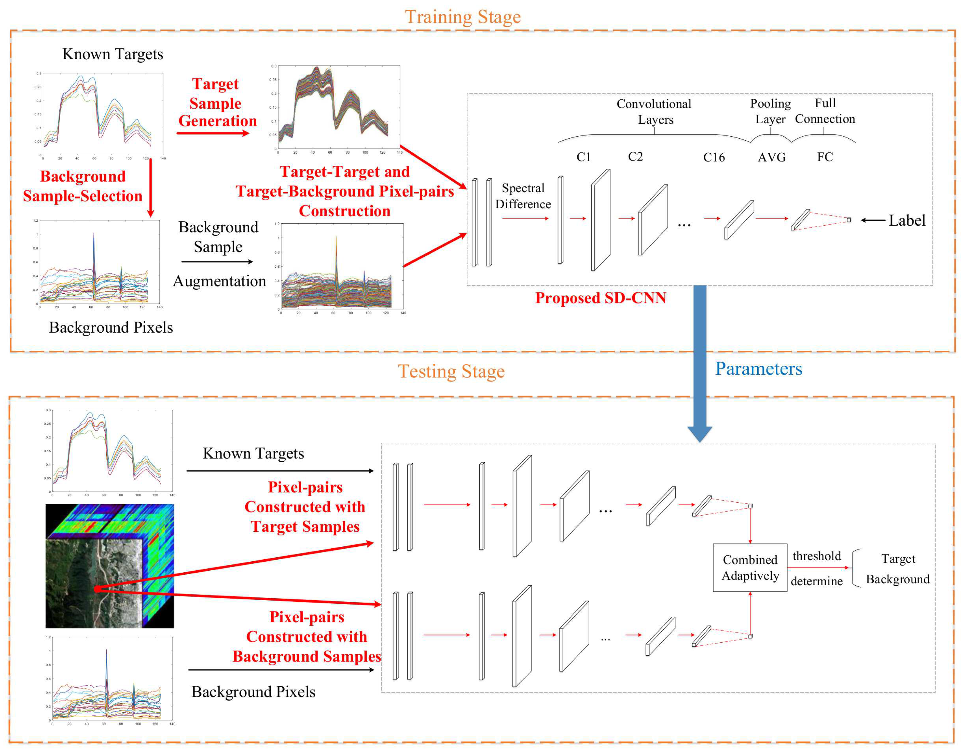
Hyperspectral image classification methods based on deep learning have been continuously developed, however, research on hyperspectral target detection based on deep learning is currently scarce. One of the difficulties of hyperspectral target detection is that available spectral signatures are usually not enough to satisfy the requirement of training deep architecture. In the light of this issue, a hyperspectral target detection framework using a deep network with data augmentation (denoted as HTD -Net) is proposed, where an improved autoencoder (AE) [31] is firstly employed to generate target signatures and select distinctive background samples that are the most different from target samples in the detecting image with the criterion of linear prediction (LP) [32]. Two types of pixel-pairs are created: one type, representing similarity, is composed of target samples; the other type, representing dissimilarity, is composed of target and background samples, which is viewed as the input of a pre-designed network architecture to learn discriminative similarity. For a testing pixel, two groups of difference constructed with target pixels and background pixels are classified by the well-trained network with results of similarity measurement. Two similarity scores are derived by averaging these two groups, and then the detection output is obtained by combining two similarity scores. Consequently, a testing pixel is claimed as a target if it is more similar to target samples than to background samples; otherwise, it is claimed as a background pixel.
The main contributions of this work are summarized as follows. First, a CNN architecture is designed to learn similarity discrimination with linear regression. Second, to solve the few-training-sample issue in the detection task, an improved AE is utilized to generate potential target signatures, and these target signatures are used to extract background samples to provide a more accurate representation of background. Third, target-target similar pixel-pairs and target-background dissimilar pixel-pairs are generated and used to train a CNN. The final detection result is obtained from considering the two types of similarity scores, where the significantly increased number of training samples (i.e., pixel-pairs) can significantly improve the detection performance.
2. Proposed Target Detection Framework
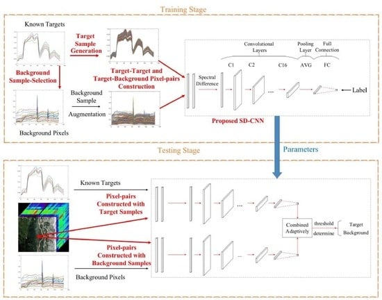
The proposed hyperspectral target detection framework is illustrated in Figure 1, which mainly includes four steps (marked as overstriking red), i.e., utilizing a modified AE to generate target samples, selecting background samples from detecting images based on LP, training a CNN using the difference between pixel-pairs, and combining the output from target and background signatures adaptively. The detailed implementation is further summarized in Algorithm 1.
| Algorithm 1 The Proposed HTD-Net |
|
2.1. Generation of Target Samples
Since target samples are usually insufficient to train a CNN, a data augmentation strategy is designed to generate more target signatures. For CNN using natural scene images, there are many ways to increase the number of samples, such as rotation, folding, adding noise, and so on. However, these methods are inappropriate for hyperspectral target detection since target signatures have known spectral information only. Rotation and folding will undoubtedly destroy spectral details and result in spectral distortion, and adding noise cannot enlarge spectral diversity. Therefore, autoencoder with generation capability is adopted, and a sample generator is built to solve the problem of insufficient target samples. Meanwhile, a loss function is used to ensure the similarity between generated and original samples.
The autoencoder (AE) is an unsupervised learning algorithm [31]. We can also consider the autoencoder as a feature learning method in a self-supervised mode, and its learning strategy can be abstracted into a convex optimization problem that minimizes reconstruction errors. A simple model of AE has two major components, i.e., an encoder and a decoder. The encoder can map the input to the hidden layer subspace through common convolution operations in deep networks, to form hidden layer features. After obtaining the hidden layer representation through the encoding operation, the decoder uses the hidden layer representation to reconstruct the input inversely. Usually, this simple AE ends up learning a low-dimensional representation when the values of the hidden layer are used. However, here, we use the values of the output layer to generate samples simulating the target signatures. The typical feature of AE is that the learning goal of its output is the input, so the training process of AE is a process in which the output continuously approaches the input. Let denote the input vector, where M is the number of input nodes. Let denote the corresponding output. The objective of the AE network is to learn an approximate relationship: . The loss function of the AE is
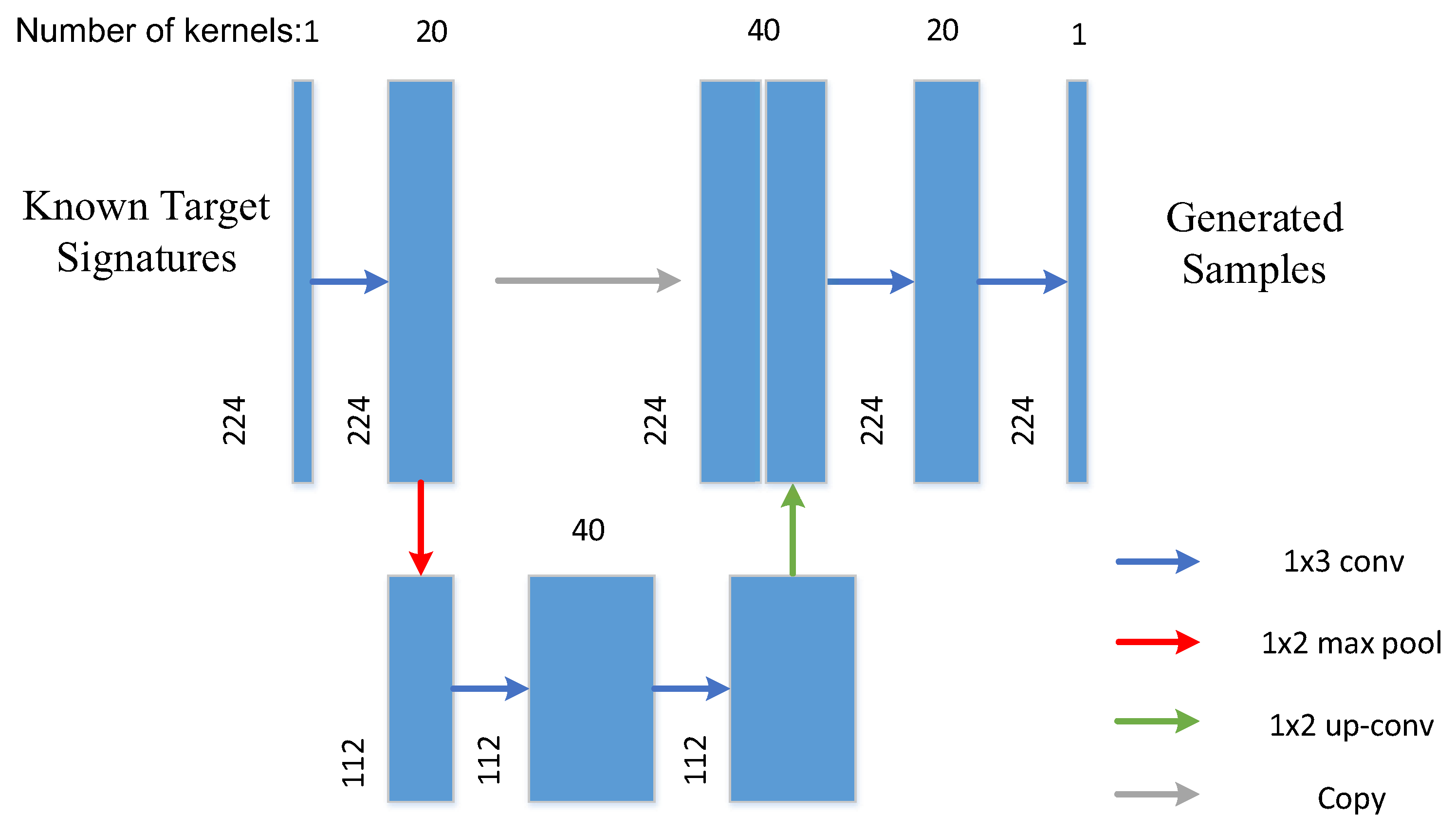
A simple AE does not fit the complex spectral curve of pixels well. In order to preserve the rich texture information of HSI, the idea from U-net [33] is borrowed, where a modified AE with a contracting path and a symmetric expanding path is designed (denoted as U-AE). The architecture of U-AE is illustrated in Figure 2, which consists of five convolutional layers, a maximum pooling layer, an upsampling layer, and a copy connection. Compared with full connection layers, the convolutional layers include fewer parameters but extract more precise features. The upsampling operator replacing the pooling operator increases the spectral resolution. In order to ensure that context can be captured, high spectral resolution features from the contracting path are combined with the upsampled output. Most noticeably, although the U-AE belongs to unsupervised learning, it needs training samples to construct the model, but it does not need to know the labels of the training data. During training, the available target and background samples in the training image are utilized for training this unsupervised network. The objective is to learn the distribution of the original data and to better fit and generate the data. When using the trained U-AE to generate samples, a small number of target pixels is selected as input data of the U-AE. The specific sample proportion will be introduced in Section 4. With fewer target sample pixels, more target sample pixels are generated to achieve data augmentation.
The comparison of generated signatures between the designed U-AE and the typical AE is shown in Figure 3. It can be seen that AE yields severe spectral distortion in the range of 1 to 50 bands, which has lost the original spectral signatures and created a new category. The generated signatures of the U-AE preserve more context and are more similar to inputs than those generated from the traditional AE.
2.2. LP-Based Background Sample Selection
For hyperspectral target detection, in order to establish an accurate background model, we further use target signatures to select background samples. The objective is to find background samples, which are the most dissimilar to target signatures in an entire image. LP can capture representative components of the spectrum, and find background samples with the largest difference from the target spectrum. These pixels are called endmembers and can be assumed as background samples. The spectral signatures of the endmembers are the most different from the target sample, which provide an accurate representation of dissimilarity between pixel-pairs. Let denote the given target spectral characteristic matrix. It is used to estimate background sample from the entire image as
where is the estimate or linear prediction of output , and is the weight vector. The linear error between the linear prediction and the expected value is expressed as
If this linear error is maximized, the difference between and will also be maximized; thus, the sample obtained can be assumed to be the background. With the least-squares solution, the weight vector can be determined as
Thus, the first background sample can be obtained by maximizing the following residual,
After obtaining , the target spectral matrix is updated as to search for . Following the same step, the entire background matrix can be found, where is the number of background samples. However, the matrix may become ill-rank after some iterations, LP cannot continue to find the next sample, so the background samples that can be found are limited. Data augmentation is employed again to enlarge the background data set. Based on the Euclidean distance, a series of samples is found closest to the background samples on the entire image, and these samples are also considered as background samples.
2.3. Construction of Training Pixel-Pairs
Pixel-pairs can be constructed by combining target samples and background samples. Two types of pixel-pairs are constructed; that is, one type of pairs selected from target samples that represents similarity, and the other type of pairs with two pixels being selected from target and background samples that represents dissimilarity. As shown in Figure 1, the pixel-pairs are constructed using target-target and target-background samples.
We discuss two strategies of learning label based on the constructed pixel-pairs:
(1) The first one is logistic regression. In particular, pixel-pairs representing similarity are labeled as 1, and the pixel-pairs representing dissimilarity are labeled as 0. The corresponding cross-entropy cost function is
where n is the batch-size, is the output of the sigmoid layer, and is the label (0 and 1).
(2) The second one is linear regression. Considering the diversity, labels of 0 and 1 cannot represent multiple similarities between pixel-pairs. Inspired by hypothesis-testing-based detection algorithms, we use the output of typical ACE to represent the similarity between pixel-pairs. Suppose is a pixel-pair after data mean removal, and the corresponding label can be computed as
where is the estimated covariance matrix of the test image. This formula has the commutative invariance property so that . The larger the value of Equation (7), the more similar the two pixels are. Here, the mean square error (MSE) is used as the cost function
where is the output of the full connection layer, and is the label. The performance of the two strategies will be compared in the following section.
2.4. Similarity-Discrimination CNN
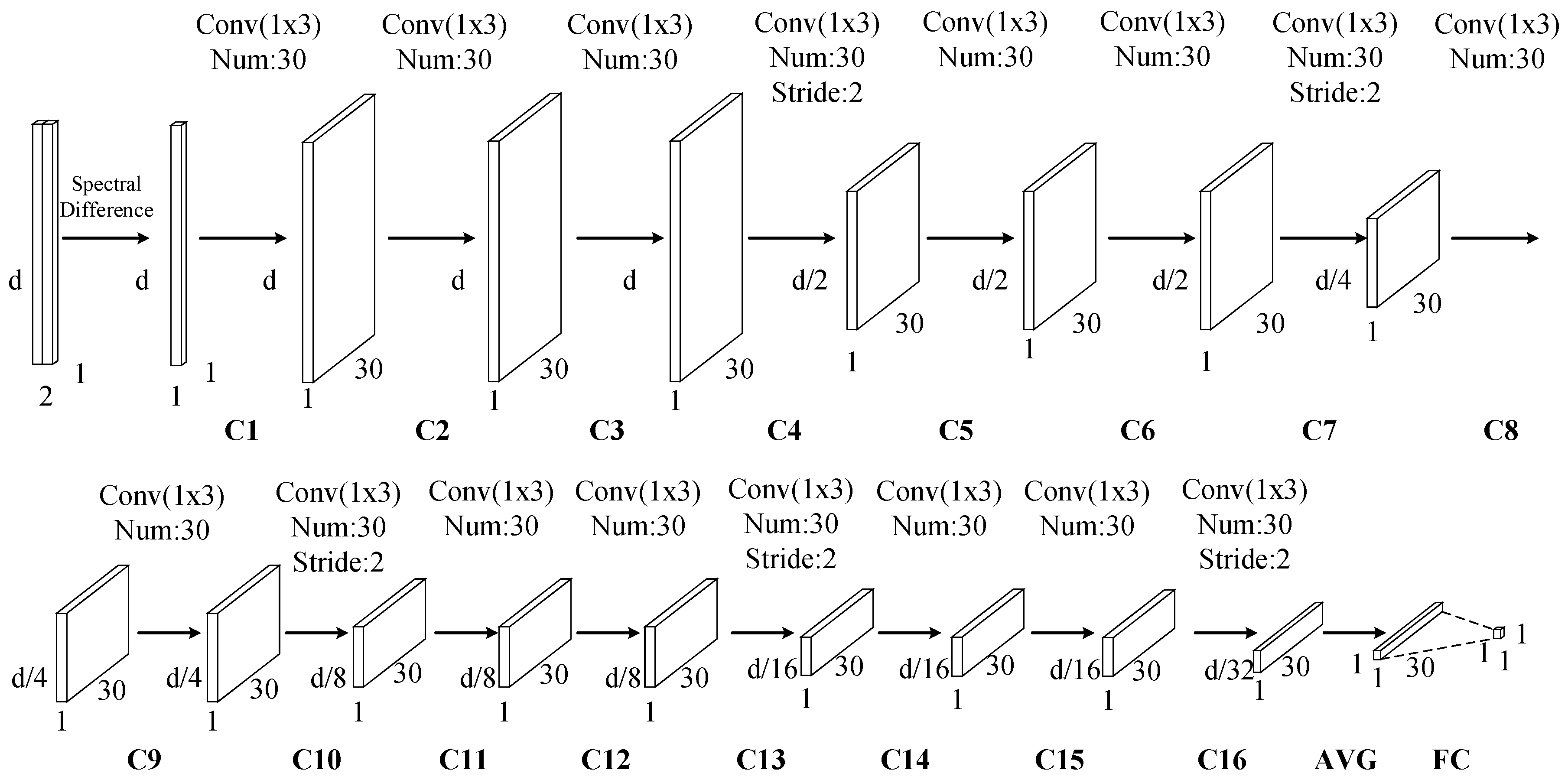
After obtaining new training data, a framework of similarity discrimination using CNN (denoted as SD-CNN) is used to extract depth features. Parameters for each layer and architecture of the designed SD-CNN are illustrated in Figure 4 and Figure 5.
In general, a typical CNN represents a feed-forward neural network that consists of various combinations of convolutional layers, max-pooling layers, and fully connected layers. In this work, we use 16 successive convolutional layers rather than stacking alternatively convolutional layers and pooling layer. After convolution, the depth features are processed by an average-pooling layer (AVG), and then its output is used as the input of a fully-connected (FC) layer. Each component in the SD-CNN is described as follows.
(1) Input Layer: the inputs to the SD-CNN are the differences of spectral signatures between pixel-pairs. Let denote the difference between pixel-pair , where is the number of spectral bands, N is the number of pixel-pairs. can be computed as
where means the absolute value operation. The objective of the SD-CNN is to decide whether the two pixels are similar or not.
(2) Convolutional Layer: due to the local connections and tied kernel weights of convolutional layers, it is easier for CNNs to train and have fewer parameters than fully-connected networks with the same number of hidden units. A conventional CNN architecture includes alternatively stacking of convolutional layers and pooling layers. However, due to the fact that pooling layers blur the discrimination among different spectral bands, it may result in information loss in the spectral dimension. Taking consider of this sake, in the designed network, the pooling layers are replaced with convolutional layers (i.e., C4, C7, C10, C13, and C16) whose kernels stride is two. There are 16 successive convolutional layers. In these convolutional layers, two kinds of kernels are used. As illustrated in Figure 4, the first one with one stride, which is denoted as blue, is padded with zeros so that the size of the output is invariable, and the second one with two strides, which is denoted as yellow, has no padding so that the number of spectral features of output is halved. The second kernels perform as the role of subsampling layers to reduce the spectral dimensionality and retain the spectral information by the convolutional operator. For example, in the first convolutional layer (C1), 30 kernels of size filter the input spectral difference, producing a tensor, and in C4, 30 kernels of size with 2 stride filter the output of C3, producing a tensor. In the following convolutional layers, the size of kernels is fixed as , and the number of kernels is fixed as 30.
(3) Average-pooling Layer and Fully-connected Layer: once the spectral dimension is desirable to use, an AVG is employed to synthesize the features of each row in the output tensor. Then all of those average is fed into the FC layer whose output is a single value.
(4) Output Layer: the output denotes the probability that a pixel belongs to the target. For logistic regression, the output of FC is usually fed into a sigmoid layer. For linear regression, this output is directly used for computing cost function. Figure 4 further lists detailed parameters in each layer.
2.5. Combined Target and Background Similarity Scores
For each testing pixel in the detecting image, pixel-pairs generated with target and background samples are individually fed into the well-trained CNN. The outputs are two sets of similarity scores. We simply average these values to generate target prediction and background prediction . The final output for target detection is calculated as
We determine whether the test pixel is the target sample by setting a threshold. In the following section, the process of determining the decision threshold is discussed. If is above the threshold , the testing pixel belongs to target; otherwise, background.
3. Analysis on Proposed Method
In this section, we analyze the advantages of the proposed HTD-Net with some state-of-the-art representation-based target detection methods and the closely-related anomaly detection method [34] using the CNN model.
3.1. Comparison with Representation-Based Detectors
In [9], a sparsity-constrained algorithm, i.e., SR-TD, was applied to detect targets of interest in hyperspectral images. Based on the sparse linear combination relationship between the test sample and the training sample, a sparse vector was constructed to help determine the category of the test sample. Based on the compressive sensing theory [35], the problem of minimizing the -norm can be transformed into a standard linear regression problem. Because it does not use of background samples, the result of target detection may be vulnerable to background interference.
Taking this problem into account, the proposed method uses both target and background samples for the testing process. In [12], combining sparse representation and cooperative representation in HSI, a target detection algorithm was proposed. Representation of test pixels is done through competitive confrontation. This method can well suppress background and highlight targets. However, this method using a combined model needs to manually adjust parameters, such as regularization parameter and window-size of selecting backgrounds, for different data to achieve an optimal result. Our proposed method, belonging to a global detector, has few parameters which has good adaptive ability to different images. Thus, the proposed HTD-Net offers better adaptability than the representation-based algorithms.
3.2. Comparison with CNN-Based Anomaly Detection
Recently, an anomaly detection framework with transferred CNN was proposed [34]. This method utilizes a reference data to generate pixel-pairs for training CNN. Considering the fact that no prior information is available in many practical cases, a dual window around the testing pixel was used to construct pixel-pairs for detection. It is worth mentioning that the test data and reference data for anomaly detection are preferably collected by the same sensor. This factor may limit practical applications of the detector.
During training, the proposed HTD-Net utilizes prior information (only a few target samples) rather than a reference data. Using known target signatures can improve the probability of detection in a low probability of false alarm. During testing, to generate a more accurate representation of the difference between pixel-pairs, we use background training data simultaneously selected by LP based on available target signatures. The two results of CNN output are combined to yield an adaptive similarity score for detection. Compared to the aforementioned anomaly detection, without using a sliding window means fewer parameters to be adjusted.
4. Experimental Results
In this section, we verify the detection performance of the proposed HTD-Net, and compare it with existing target detection algorithms, such as the target detector based on sparse representation (SR-TD), the target detector based on collaborative representation (CR-TD), and the traditional ACE [7]. In target detection tasks, receiver-operating-characteristic (ROC) cite Hanley1983A curve is an effective method to evaluate the detection effect quantitatively. The performance of these detectors was evaluated by quantifying the area under the ROC curve (AUC).
4.1. Hyperspectral Data
The first dataset is from the Moffett Field, California, at the southern end of the San Francisco Bay, which was collected by AVIRIS sensors. As illustrated in Figure 6, the scene consists of pixels, has 224 bands, spans a wavelength interval of 0.4- to 2.5-m, and has a spatial resolution of about 20 m [36]. Here, the total number of target pixels in the scene is 59. Five target samples are selected as known.
The second dataset is from the World Trade Center (WTC) area in New York City, which was collected by AVIRIS sensors five days after WTC collapsed by terrorist attacks [37]. As shown in Figure 7, the scene consists of pixels, has 224 bands. There are 91 targets in burned areas, and 8 of them are used as known target samples.
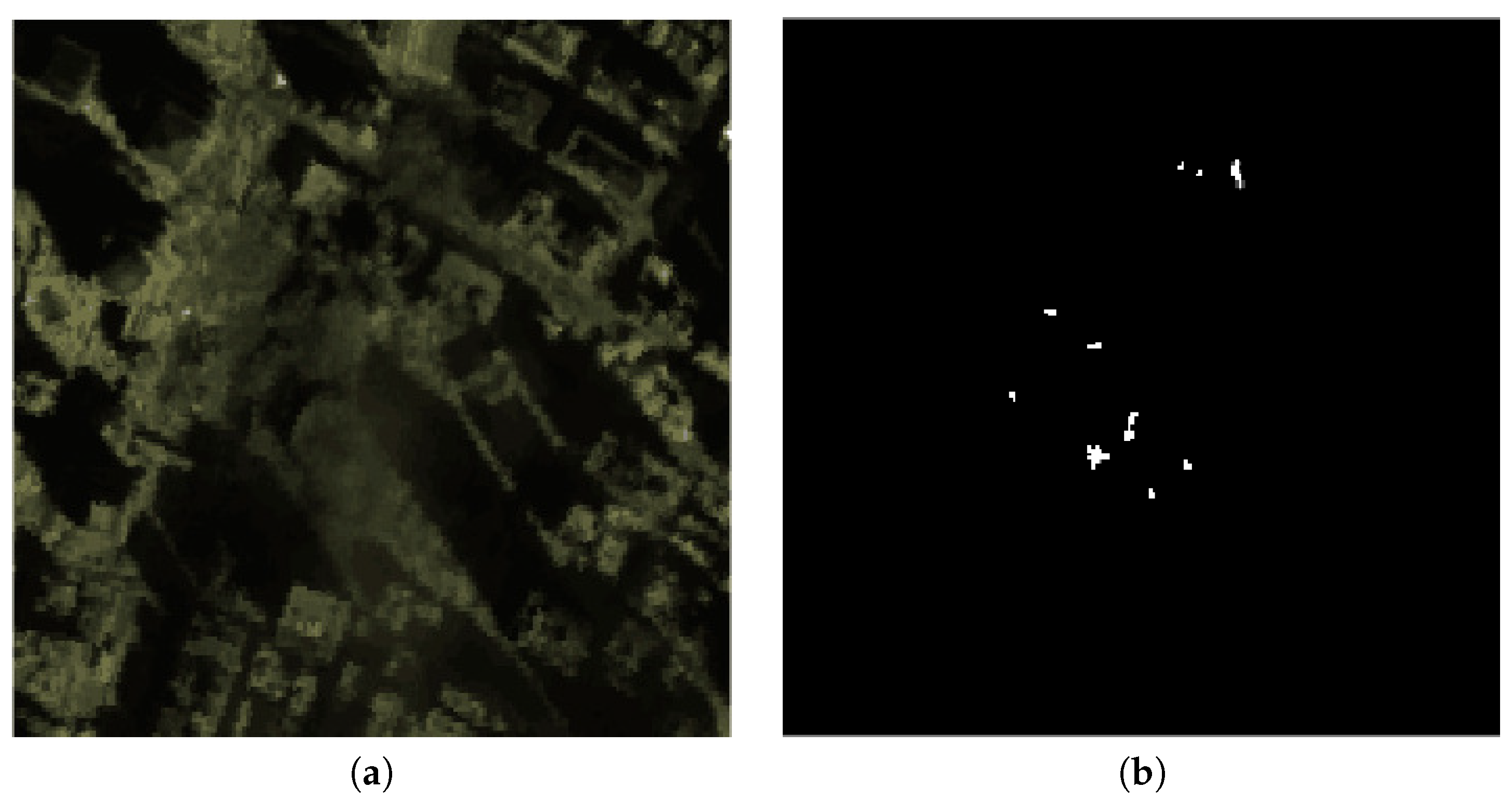
The third dataset is from the Hyperspectral Digital Imagery Collection Experiment (Hydice Forest). As shown in Figure 8, the scene consists of pixels, has 210 bands(169 bands left after removing water-absorption bands.), spans a wavelength interval of 0.4- to 2.5-m, and has a spatial resolution of about 1.56 m. 19 target pixels are corresponding to 15 target panels, and 5 of them are used as known target samples.
The fourth dataset is from the HyMap airborne hyperspectral imaging sensor [38], which covers an area in Cooke City, MT. The scene consists of pixels, has 126 bands, spans a wavelength interval of 0.4- to 2.5-m, and has a spatial resolution of about 3 m. There are 7 types of targets, of which 4 are fabric panel targets and 3 are vehicle targets. In our experiment, the image is cropped to a sub-image of size , and 4 types of fabric panel targets are detected, including 118 target samples, as shown in Figure 9. Four of them are used as known target samples.
4.2. Parameter Setting for Deep Network
In order to obtain a well-trained CNN, there are several essential parameters, such as learning rate, batch size, and a minimum of dequeue, which need to be well tuned. The learning rate determines the convergence speed of the network. The batch size controls the number of input data per step. The minimum of dequeue defines how big a buffer we will randomly sample from, where a larger value means better shuffling but slower speed and more space memory needed. Furthermore, we also discuss the relationship between the numbers of generated target samples and selected background samples.
According to our empirical study, the batch size is set as 256 to take the most use of parallel computing ability of GPU for both linear and logistic models. The choice of a minimum of dequeue depends on the computing capacity. The value is set by the following criterion: , where the capacity is 50,000 in our experiments. For the learning rate, the learning procedure is too fast to have a convergence when it is too large, while the model needs many iterations to converge when the learning rate is low. Therefore, a suitable compromise method is to first set the learning rate to a relatively large value (such as 0.01), and adjust the reduction according to the fluctuation of the learning curve. After the training data is enlarged, part of the data is used as a validation set to estimate the optimal parameters.
The impact of imbalanced training data on hyperspectral image classification performance has been studied in [39]. It indicates that if the training data is unbalanced, it will negatively affect the performance of the CNN, but the balanced data under the same conditions will be better [40]. Therefore, to balance the training data, the number of similarity samples is twice as many as dissimilarity samples, then the number of samples representing similarity and non-similarity is guaranteed to be the same. In this paper, we generate 1000 target samples and find 500 background samples. The number of similarity pixel-pairs is as high as 499,500 (i.e., ), and the number of dissimilarity pixel-pairs is 500,000 (i.e., ).
4.3. Comparison between Linear and Logistic Strategies
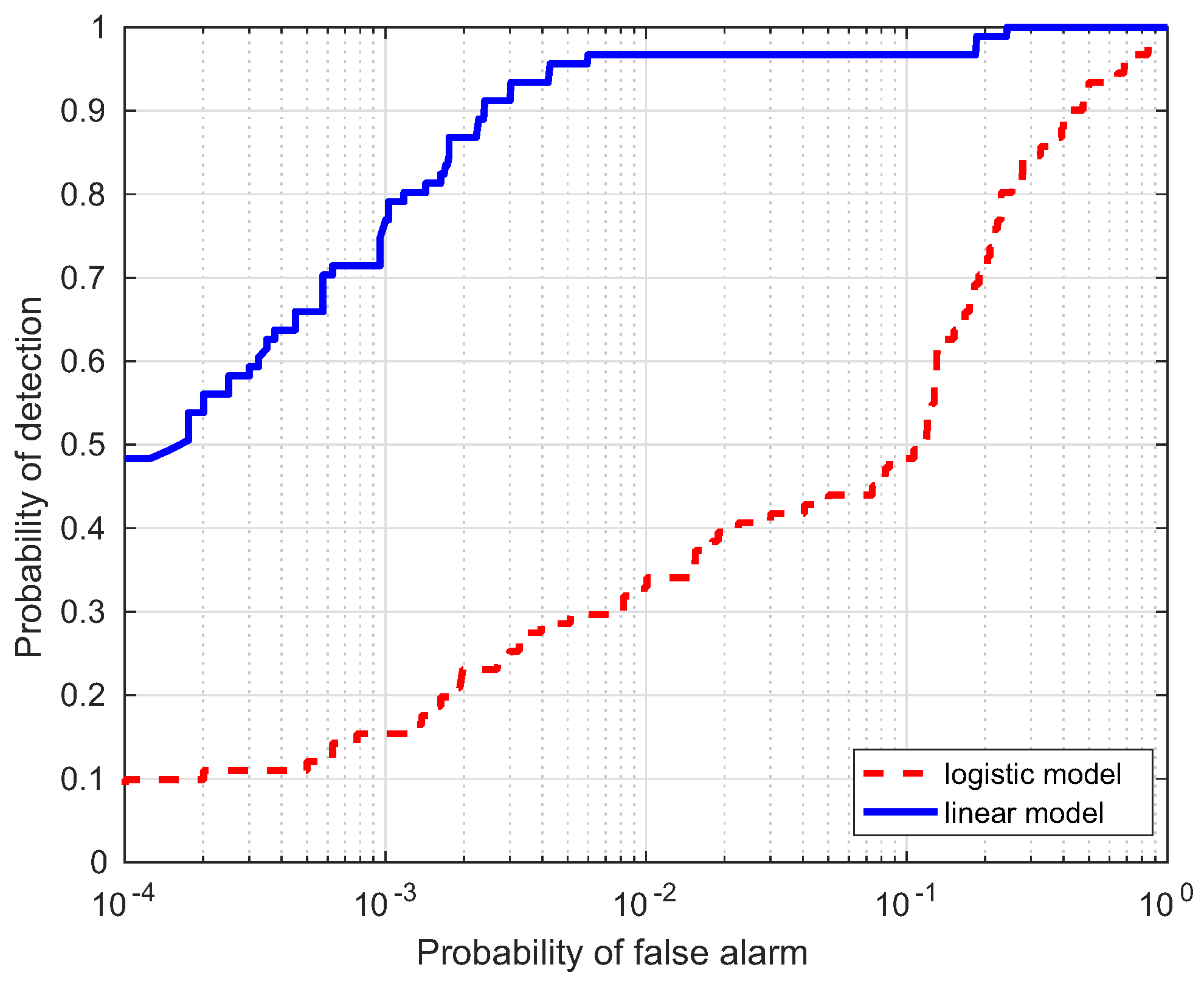
In this section, a comparison for the two strategies is investigated, i.e., linear and logistic regression, which are denoted as the linear model and logistic model, respectively. Table 1 lists the AUC performance(%) of the two models for the four data, where Target Samples denotes the case using targets only, Background Samples denotes the case using backgrounds only, and Combined Samples denotes the case combing the two results. It is interesting to notice that the AUC(%) values from the linear model are larger than those from the logistic model. ROC curves of the two models are illustrated to further evaluate the performance in Figure 10, Figure 11, Figure 12 and Figure 13. Compared with the logistic model, the linear model offers a higher probability of detection for the four experimental data. From these results, the linear model is superior to the logistic model, which verifies the assumption in the previous section. Therefore, the linear regression is adopted as the learning model in the proposed HTD-Net.
4.4. Comparison Performance with Traditional Methods
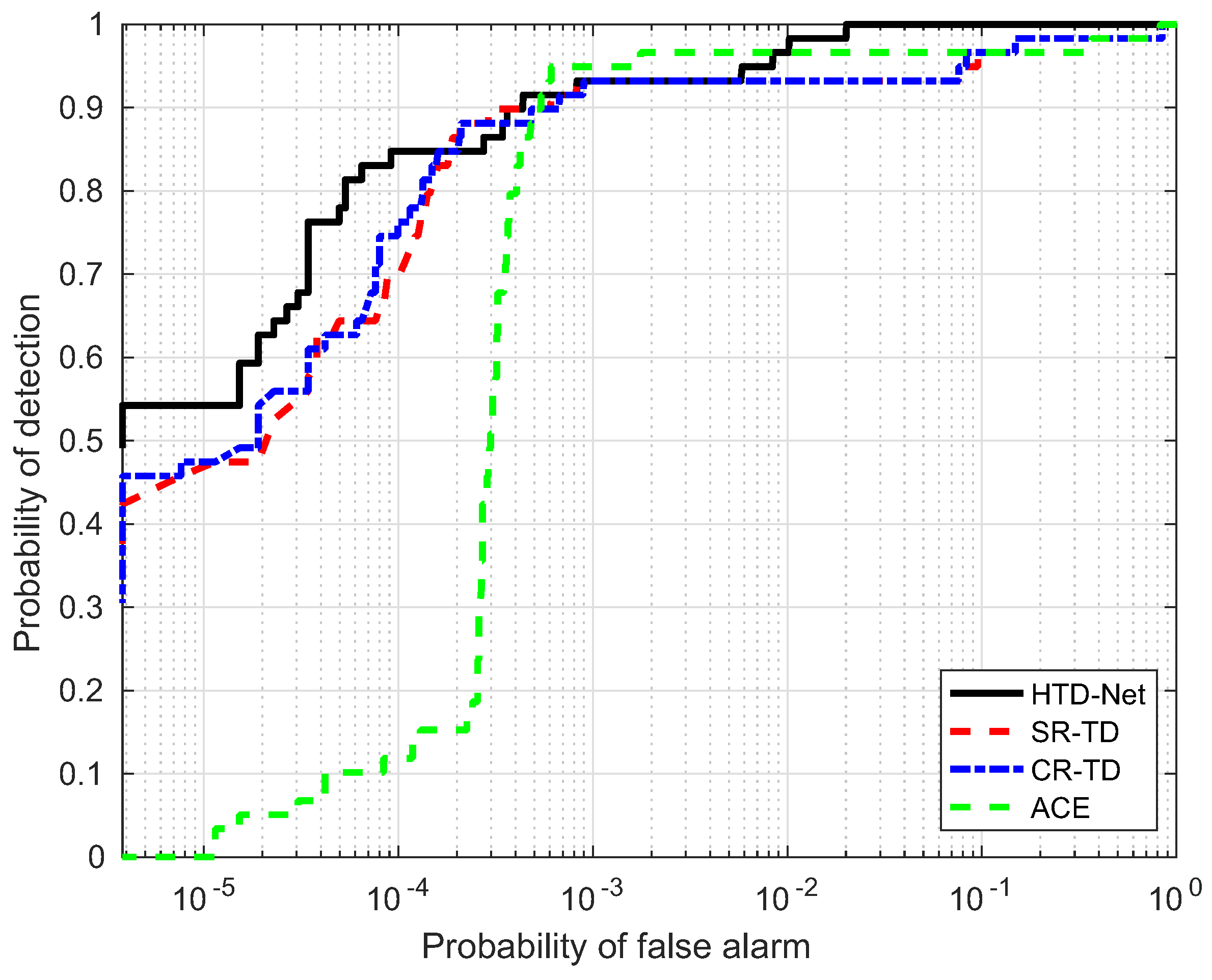
For a fair comparison, we need to adjust the parameters for SR-TD, CR-TD, and ACE to achieve their optimal state, e.g., the size of the double window and regularization parameters. The size of the double window determines the number of background samples selected by SR-TD and CR-TD, and the regularization parameters control the balance between the residual terms and the weight criteria. Figure 14, Figure 15, Figure 16 and Figure 17 shows the ROC curves of the four detectors, all adjusted to the optimal parameter state, which verifies the superiority of our proposed HTD-Net.
In most situations, the proposed HTD-Net is superior to other detectors. For instance, the HTD-Net offers a better probability of detection (i.e., ) when the false alarm rate (i.e., ) locates in a relatively small range (such as to ), which is considered as practical application value in Figure 16.
The AUC performance(%) comparison is also listed in Table 2. From the results, the AUC value of the proposed HTD-Net is always the largest. Take the HyMap data for example, the AUC value is 96.03%, with an improvement of approximately 5% when compared to the SR-TD and CR-TD. In addition, of the HTD-Net achieves 1.00 even for small . Figure 18, Figure 19 and Figure 20 further show that the detection maps when is a small value (e.g., 0.0001 or 0.002) and reaches the maximum. The proposed HTD-Net still reaches the highest value and the best overall performance. When we fix to a desired value, a suitable threshold can be determined.
The statistical significance of the performance difference between different detectors is compared in Table 3. We use Wilcoxon statistics to calculate a series of values. At a confidence level, If Z > 1.96, it means statistically significant. Similarly, At a confidence level, If Z > 2.58, it means statistically significant. When the significance level (i.e., the p value) is less than 0.05, the difference between the two detectors proves to be significant. Obviously, in addition to the Hydice Forest data, the proposed HTD-Net has better statistical significance at (and/or ) confidence level. In addition, the proposed HTD-Net is inclined to produce better performance when the size of the detecting image is large.
Finally, the computational complexity of the above detection methods is discussed. All experiments are performed on an Intel(R) Core(TM) i7-3770 CPU machine with 16GB of RAM based on Python language and Tensorflow library. The execution time of different detectors (in seconds) is compared in Table 4. The results of Table 4 show that the proposed HTD-Net is time-consuming. There are two reasons for this result. First, compared with the traditional method, the method of using deep networks to learn data will inevitably consume more time. Deep learning takes advantage of large data samples, which requires more computing resources to extract features for better data fitting and higher detection performance. This inevitably brings about increased computational complexity. The proposed method effectively improves the detection performance at the sacrifice of computing cost. In addition, the amount of data generated by UAE is large, which greatly expands the sample size. The rich input effectively improves the training accuracy, but it also greatly increases training costs.
5. Conclusions
In this paper, a CNN-based algorithm using only few target signatures has been proposed for hyperspectral target detection, denoted as HTD-Net. To ensure sufficient samples to train the CNN, a modified AE was developed to generate more potential target signatures, based on which background samples were selected with the LP strategy to generate an accurate representation of background. Then, the training pixel-pairs were constructed by target and background samples, as the inputs to a designed SD-CNN architecture. In the testing procedure, for each pixel to be labeled, pixel-pairs constructed with target and background samples were classified by the well-trained network. The average similarity scores from the two branches of the network were then directly combined to yield the final output. Experimental results show that the proposed HTD-Net significantly outperformed the traditional ACE, and the state-of-the-art SR-TD, and CR-TD. Although a certain amount of computational cost is sacrificed, the sufficient amount of data ensures the effectiveness of the training network and reduces the training overfitting phenomenon caused by data scarcity to a certain extent. The proposed HTD-Net is suitable for situations where data is difficult to obtain and marked samples are scarce. Considering that real-time detection in practice is more concerned with detection time and network training can be designed as an offline process, the trained network may be applicable to detect targets in real-time from similar image scenes, which will be investigated in our future work. In addition, parallel algorithms will be designed with high-performance computing facilities to improve efficiency, and lightweight network models will be tested in the trade-off between detection accuracy and computational cost.
Author Contributions
All authors conceived and designed the study. G.Z. and S.Z. carried out the experiments. All authors discussed the basic structure of the manuscript, S.Z., W.L. and Q.D. finished the first draft. W.L., Q.D., Q.R. and R.T. reviewed and edited the draft. All authors have read and agreed to the published version of the manuscript.
Acknowledgments
This work was supported by the National Natural Science Foundation of China under Grants No. NSFC-61922013, U1833203, 61421001.
Conflicts of Interest
The authors declare no conflict of interest.
References
- Eismann, M.T.; Stocker, A.D.; Nasrabadi, N.M. Automated Hyperspectral Cueing for Civilian Search and Rescue. Proc. IEEE 2009, 97, 1031–1055. [Google Scholar] [CrossRef]
- Datt, B.; McVicar, T.R.; Van Niel, T.G.; Jupp, D.L.; Pearlman, J.S. Preprocessing EO-1 Hyperion hyperspectral data to support the application of agricultural indexes. IEEE Trans. Geosci. Remote Sens. 2003, 41, 1246–1259. [Google Scholar] [CrossRef] [Green Version]
- Hörig, B.; Kühn, F.; Oschütz, F.; Lehmann, F. HyMap hyperspectral remote sensing to detect hydrocarbons. Int. J. Remote Sens. 2001, 22, 1413–1422. [Google Scholar] [CrossRef]
- Jin, X.; Paswaters, S.; Cline, H. A comparative study of target detection algorithms for hyperspectral imagery. Proc. SPIE Int. Soc. Opt. Eng. 2009, 7334, 73341W. [Google Scholar]
- Robey, F.C.; Fuhrmann, D.R.; Kelly, E.J.; Nitzberg, R. A CFAR adaptive matched filter detector. IEEE Trans. Aerosp. Electron. Syst. 1992, 28, 208–216. [Google Scholar] [CrossRef] [Green Version]
- Funk, C.C.; Theiler, J.; Roberts, D.A.; Borel, C.C. Clustering to improve matched filter detection of weak gas plumes in hyperspectral thermal imagery. IEEE Trans. Geosci. Remote Sens. 2001, 39, 1410–1420. [Google Scholar] [CrossRef] [Green Version]
- Kraut, S.; Scharf, L.L.; Butler, R.W. The adaptive coherence estimator: A uniformly most-powerful-invariant adaptive detection statistic. IEEE Trans. Signal Process. 2005, 53, 427–438. [Google Scholar] [CrossRef]
- Matteoli, S.; Acito, N.; Diani, M.; Corsini, G. Local approach to orthogonal subspace-based target detection in hyperspectral images. In Proceedings of the Workshop on Hyperspectral Image and Signal Processing: Evolution in Remote Sensing, Grenoble, France, 26–28 August 2009; pp. 1–4. [Google Scholar]
- Chen, Y.; Nasrabadi, N.M.; Tran, T.D. Sparse Representation for Target Detection in Hyperspectral Imagery. IEEE J. Sel. Top. Signal Process. 2011, 5, 629–640. [Google Scholar] [CrossRef]
- Du, B.; Zhang, Y.; Zhang, L.; Tao, D. Beyond the Sparsity-Based Target Detector: A Hybrid Sparsity and Statistics-Based Detector for Hyperspectral Images. IEEE Trans. Image Process. 2016, 25, 5345–5357. [Google Scholar] [CrossRef]
- Wang, T.; Zhang, H.; Lin, H.; Jia, X. A Sparse Representation Method for a Priori Target Signature Optimization in Hyperspectral Target Detection. IEEE Access 2018, 6, 3408–3424. [Google Scholar] [CrossRef]
- Li, W.; Du, Q.; Zhang, B. Combined sparse and collaborative representation for hyperspectral target detection. Pattern Recognit. 2015, 48, 3904–3916. [Google Scholar] [CrossRef]
- Li, C.; Gao, L.; Wu, Y.; Zhang, B.; Plaza, J.; Plaza, A. A real-time unsupervised background extraction-based target detection method for hyperspectral imagery. J. Real Time Image Process. 2018, 15, 597–615. [Google Scholar] [CrossRef]
- Li, W.; Zhao, M.; Deng, X.; Li, L.; Zhang, W. Infrared Small Target Detection Using Local and Nonlocal Spatial Information. IEEE J. Sel. Top. Appl. Earth Obs. Remote Sens. 2019, 12, 3677–3689. [Google Scholar] [CrossRef]
- Tao, R.; Zhao, X.; Li, W.; Li, H.C.; Du, Q. Hyperspectral Anomaly Detection by Fractional Fourier Entropy. IEEE J. Sel. Top. Appl. Earth Obs. Remote Sens. 2019, 12, 4920–4929. [Google Scholar] [CrossRef]
- Ma, X.; Geng, J.; Wang, H. Hyperspectral image classification via contextual deep learning. Eurasip J. Image Video Process. 2015, 2015, 20. [Google Scholar] [CrossRef] [Green Version]
- Zou, Q.; Ni, L.; Zhang, T.; Wang, Q. Deep Learning Based Feature Selection for Remote Sensing Scene Classification. IEEE Geosci. Remote Sens. Lett. 2015, 12, 2321–2325. [Google Scholar] [CrossRef]
- Chen, Y.; Lin, Z.; Zhao, X.; Wang, G.; Gu, Y. Deep Learning-Based Classification of Hyperspectral Data. IEEE J. Sel. Top. Appl. Earth Obs. Remote Sens. 2014, 7, 2094–2107. [Google Scholar] [CrossRef]
- Chen, Y.; Zhao, X.; Jia, X. Spectral Spatial Classification of Hyperspectral Data Based on Deep Belief Network. IEEE J. Sel. Top. Appl. Earth Obs. Remote Sens. 2015, 8, 2381–2392. [Google Scholar] [CrossRef]
- Zhao, W.; Du, S. Spectral Spatial Feature Extraction for Hyperspectral Image Classification: A Dimension Reduction and Deep Learning Approach. IEEE Trans. Geosci. Remote Sens. 2016, 54, 4544–4554. [Google Scholar] [CrossRef]
- Ma, X.; Wang, H.; Geng, J. Spectral Spatial Classification of Hyperspectral Image Based on Deep Auto-Encoder. IEEE J. Sel. Top. Appl. Earth Obs. Remote Sens. 2016, 9, 4073–4085. [Google Scholar] [CrossRef]
- Wang, L.; Zhang, J.; Liu, P.; Choo, K.K.R.; Huang, F. Spectral–spatial multi-feature-based deep learning for hyperspectral remote sensing image classification. Soft Comput. 2017, 21, 213–221. [Google Scholar] [CrossRef]
- Zhong, Z.; Li, J.; Luo, Z.; Chapman, M. Spectral-Spatial Residual Network for Hyperspectral Image Classification: A 3-D Deep Learning Framework. IEEE Trans. Geosci. Remote Sens. 2018, 56, 847–858. [Google Scholar] [CrossRef]
- Hu, W.; Huang, Y.; Li, W. Deep Convolutional Neural Networks for Hyperspectral Image Classification. J. Sens. 2015, 2015, 1–12. [Google Scholar] [CrossRef] [Green Version]
- Slavkovikj, V.; Verstockt, S.; De Neve, W.; Van Hoecke, S.; Van de Walle, R. Hyperspectral image classification with convolutional neural networks. In Proceedings of the 23rd ACM International Conference on Multimedia; ACM: New York, NY, USA, 2015; pp. 1159–1162. [Google Scholar]
- Makantasis, K.; Karantzalos, K.; Doulamis, A.; Doulamis, N. Deep supervised learning for hyperspectral data classification through convolutional neural networks. In Proceedings of the 2015 IEEE International Geoscience and Remote Sensing Symposium (IGARSS), Milan, Italy, 26–31 July 2015; pp. 4959–4962. [Google Scholar]
- Yu, S.; Jia, S.; Xu, C. Convolutional neural networks for hyperspectral image classification. Neurocomputing 2017, 219, 88–98. [Google Scholar] [CrossRef]
- Li, W.; Wu, G.; Zhang, F.; Du, Q. Hyperspectral Image Classification Using Deep Pixel-Pair Features. IEEE Trans. Geosci. Remote Sens. 2017, 55, 844–853. [Google Scholar] [CrossRef]
- Yang, J.; Zhao, Y.Q.; Chan, J.C.W. Learning and Transferring Deep Joint Spectral-Spatial Features for Hyperspectral Classification. IEEE Trans. Geosci. Remote Sens. 2017, 55, 4729–4742. [Google Scholar] [CrossRef]
- Mei, S.; Ji, J.; Hou, J.; Li, X.; Du, Q. Learning Sensor-Specific Spatial-Spectral Features of Hyperspectral Images via Convolutional Neural Networks. IEEE Trans. Geosci. Remote Sens. 2017, 55, 4520–4533. [Google Scholar] [CrossRef]
- Hinton, G.E.; Salakhutdinov, R.R. Reducing the dimensionality of data with neural networks. Science 2006, 313, 504–507. [Google Scholar] [CrossRef] [Green Version]
- Du, Q.; Yang, H. Similarity-Based Unsupervised Band Selection for Hyperspectral Image Analysis. IEEE Geosci. Remote Sens. Lett. 2008, 5, 564–568. [Google Scholar] [CrossRef]
- Ronneberger, O.; Fischer, P.; Brox, T. U-net: Convolutional networks for biomedical image segmentation. In International Conference on Medical Image Computing and Computer-Assisted Intervention; Springer: Cham, Switzerland, 2015; pp. 234–241. [Google Scholar]
- Li, W.; Wu, G.; Du, Q. Transferred Deep Learning for Anomaly Detection in Hyperspectral Imagery. IEEE Geosci. Remote Sens. Lett. 2017, 14, 597–601. [Google Scholar] [CrossRef]
- Baraniuk, R.G. Compressive sensing [lecture notes]. IEEE Signal Process. Mag. 2007, 24, 118–121. [Google Scholar] [CrossRef]
- Du, Q.; Zhu, W.; Fowler, J.E. Anomaly-based hyperspectral image compression. In Proceedings of the IGARSS 2008—2008 IEEE International Geoscience and Remote Sensing Symposium, Boston, MA, USA, 7–11 July 2008; Volume 2. [Google Scholar] [CrossRef] [Green Version]
- Plaza, A.; Du, Q.; Chang, Y.L.; King, R.L. High performance computing for hyperspectral remote sensing. IEEE J. Sel. Top. Appl. Earth Obs. Remote Sens. 2011, 4, 528–544. [Google Scholar] [CrossRef]
- Snyder, D.; Kerekes, J.; Fairweather, I.; Crabtree, R. Development of a Web-Based Application to Evaluate Target Finding Algorithms. In Proceedings of the IGARSS 2008—2008 IEEE International Geoscience and Remote Sensing Symposium, Boston, MA, USA, 7–11 July 2008; pp. II-915–II-918. [Google Scholar]
- Li, J.; Du, Q.; Li, Y.; Li, W. Hyperspectral Image Classification With Imbalanced Data Based on Orthogonal Complement Subspace Projection. IEEE Trans. Geosci. Remote Sens. 2018, 56, 3838–3851. [Google Scholar] [CrossRef]
- Hensman, P.; Masko, D. The Impact of Imbalanced Training Data for Convolutional Neural Networks; Degree Project in Computer Science; KTH Royal Institute of Technology: Stockholm, Sweden, 2015. [Google Scholar]
Figure 1.
Flowchart of the proposed HTD -Net framework for hyperspectral target detection.

Figure 2.
The architecture of the U-AE (It is assumed that the selected dataset consists of 224 spectral bands).
Figure 2.
The architecture of the U-AE (It is assumed that the selected dataset consists of 224 spectral bands).

Figure 3.
Comparison of generated signatures between U-AE and autoencoder (AE) (a) Input samples, (b) Generated signatures of the traditional AE, and (c) Generated signatures of U-AE.
Figure 3.
Comparison of generated signatures between U-AE and autoencoder (AE) (a) Input samples, (b) Generated signatures of the traditional AE, and (c) Generated signatures of U-AE.
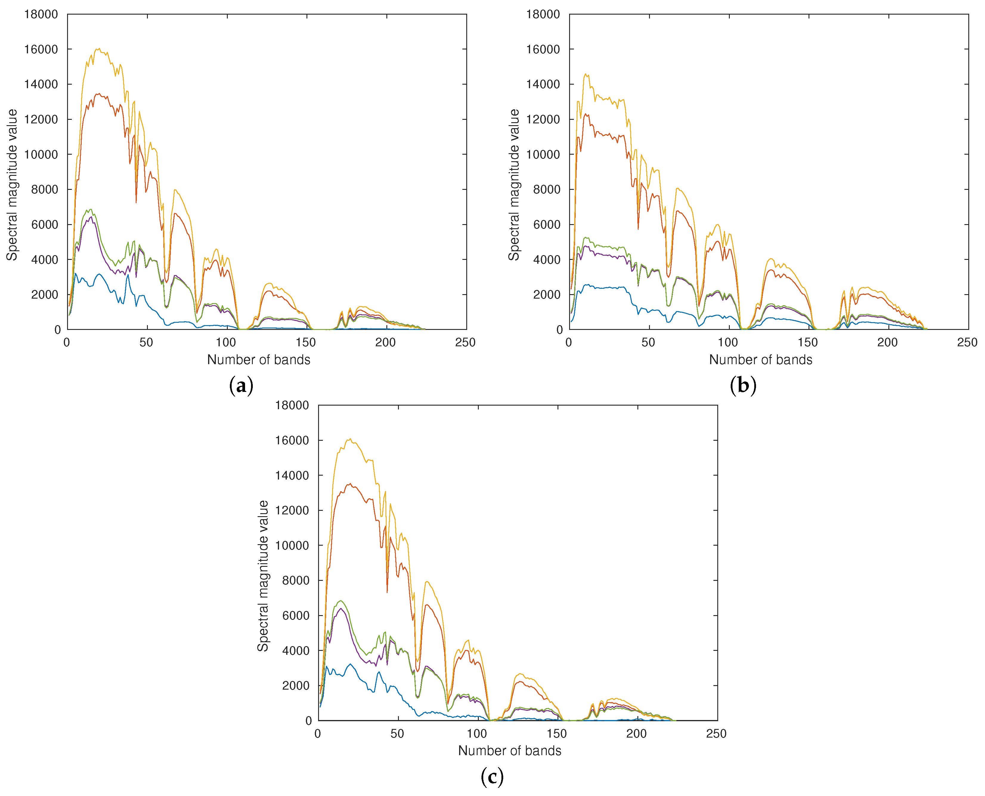
Figure 4.
Parameters for each layer of the designed similarity discrimination-convolutional neural network (SD-CNN).
Figure 4.
Parameters for each layer of the designed similarity discrimination-convolutional neural network (SD-CNN).
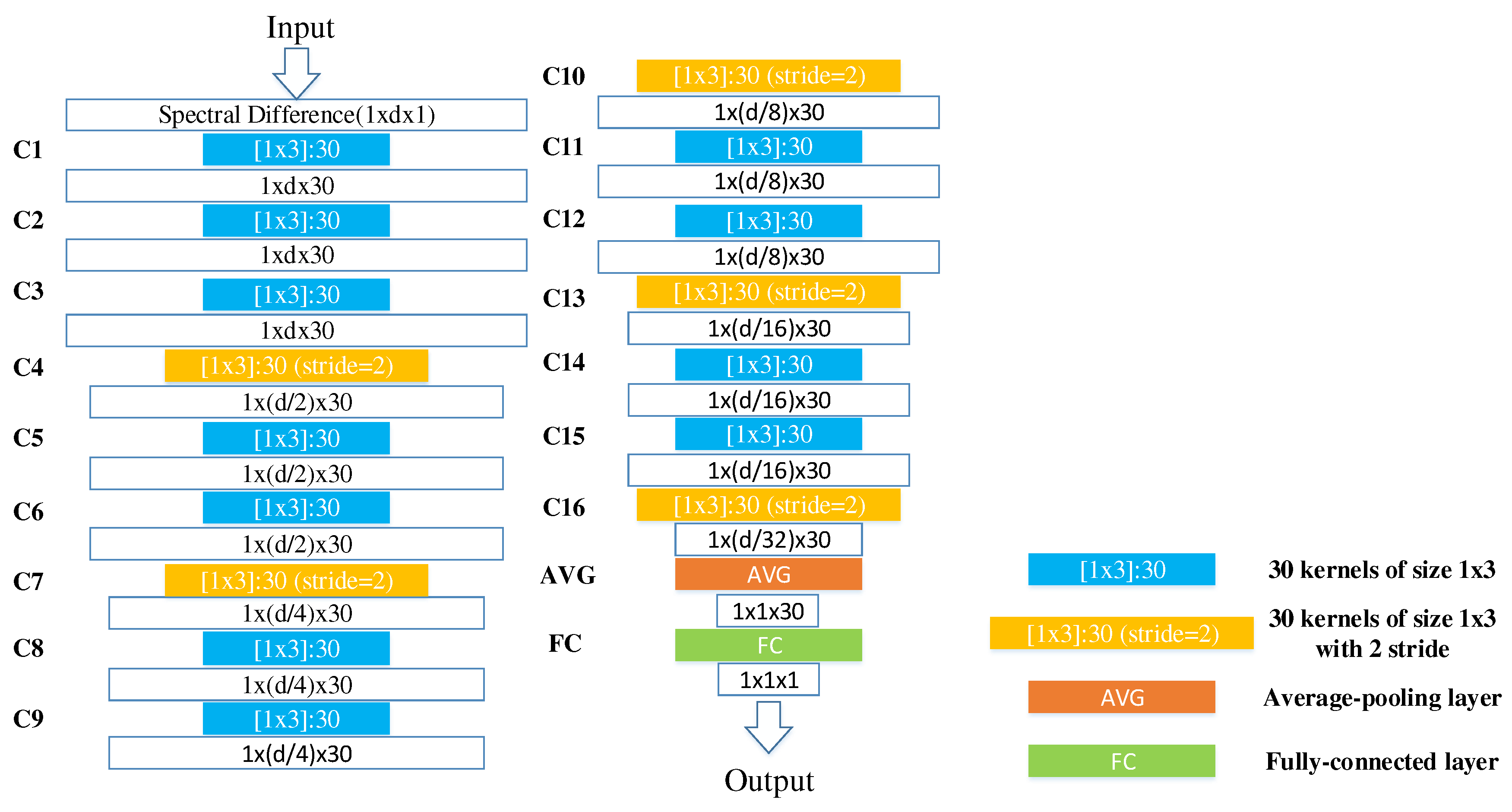
Figure 5.
Architecture of the designed SD-CNN.

Figure 6.
The Moffett Field scene with 59 target pixels (a) Pseudo-color Image (b) ground-truth map.
Figure 6.
The Moffett Field scene with 59 target pixels (a) Pseudo-color Image (b) ground-truth map.

Figure 7.
The World Trade Center (WTC) scene with 91 anomalous pixels (a) Pseudo-color Image (b) ground-truth map.
Figure 7.
The World Trade Center (WTC) scene with 91 anomalous pixels (a) Pseudo-color Image (b) ground-truth map.

Figure 8.
The Hydice Forest scene with 19 target pixels (a) Pseudo-color Image. (b) ground-truth map.
Figure 8.
The Hydice Forest scene with 19 target pixels (a) Pseudo-color Image. (b) ground-truth map.
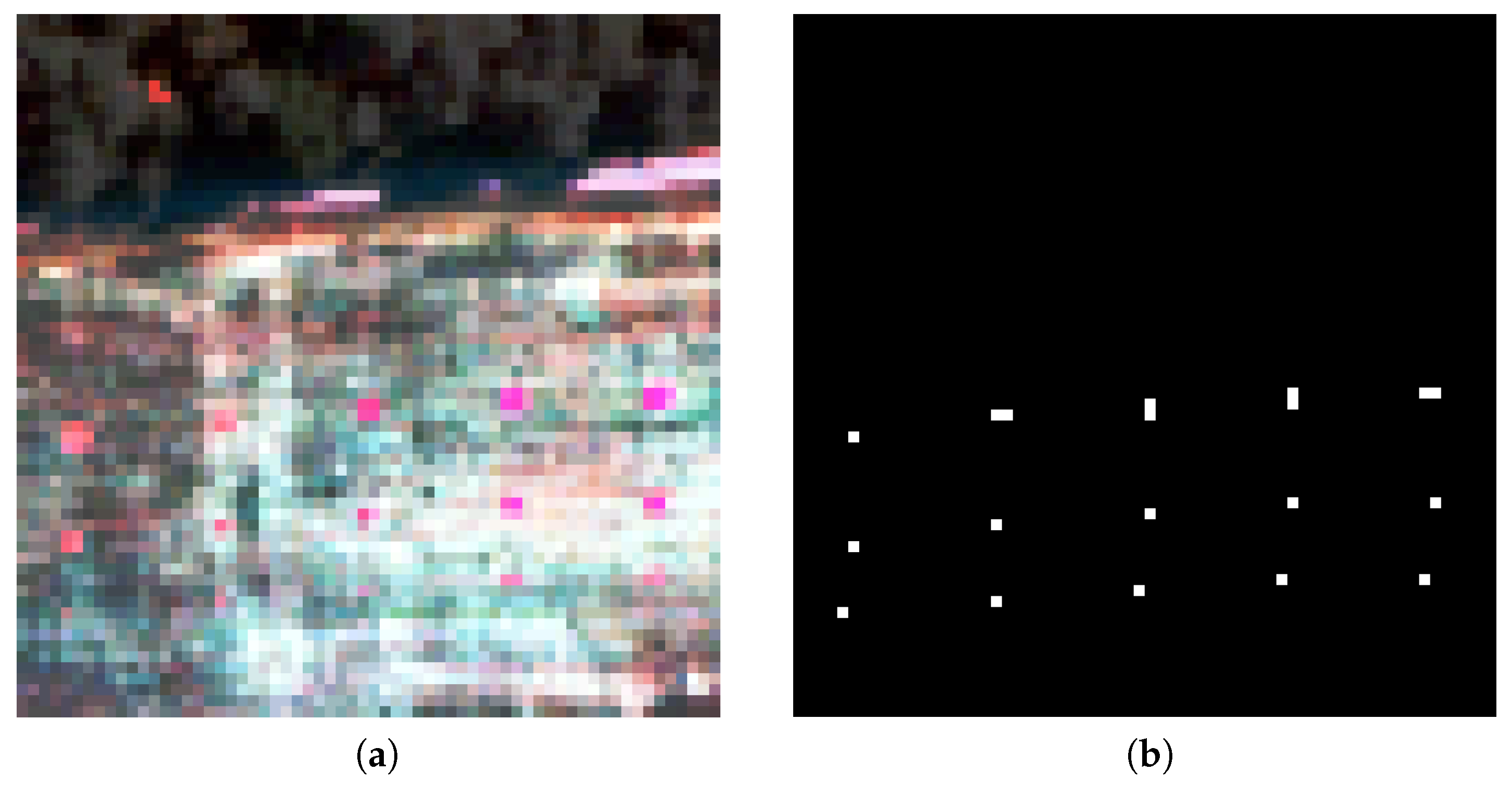
Figure 9.
The HyMap scene with 118 target pixels (a) Pseudo-color Image. (b) ground-truth map.

Figure 10.
Receiver-operating-characteristic (ROC) comparison of the two regression models for the Moffett Filed data.
Figure 10.
Receiver-operating-characteristic (ROC) comparison of the two regression models for the Moffett Filed data.

Figure 11.
ROC comparison of the two regression models for the WTC data.

Figure 12.
ROC comparison of the two regression models for the Hydice Forest data.
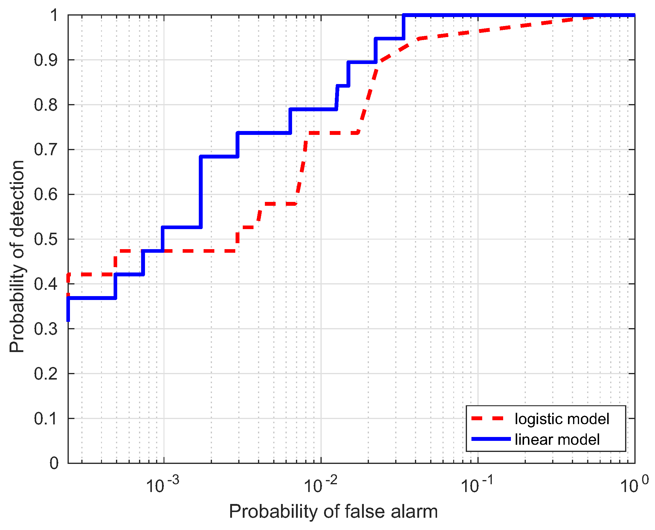
Figure 13.
ROC comparison of the two regression models for the HyMap data.

Figure 14.
ROC performance of the proposed method for the Moffett Filed data.

Figure 15.
ROC performance of the proposed method for the WTC data.
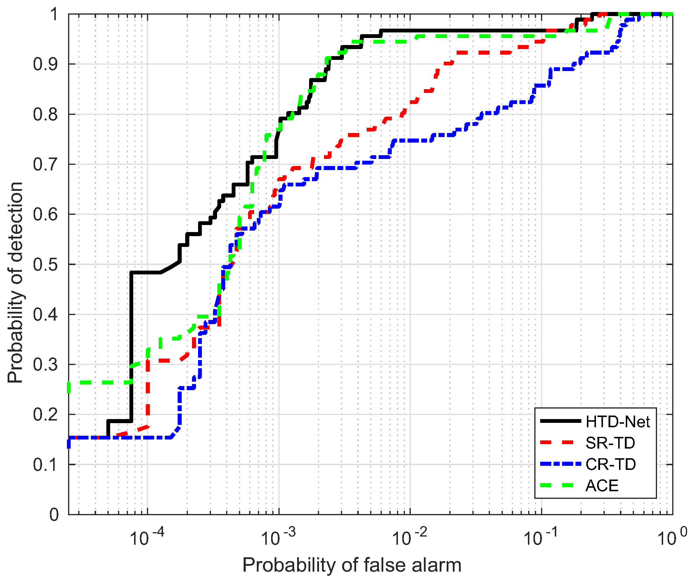
Figure 16.
ROC performance of the proposed method for the Hydice Forest data.
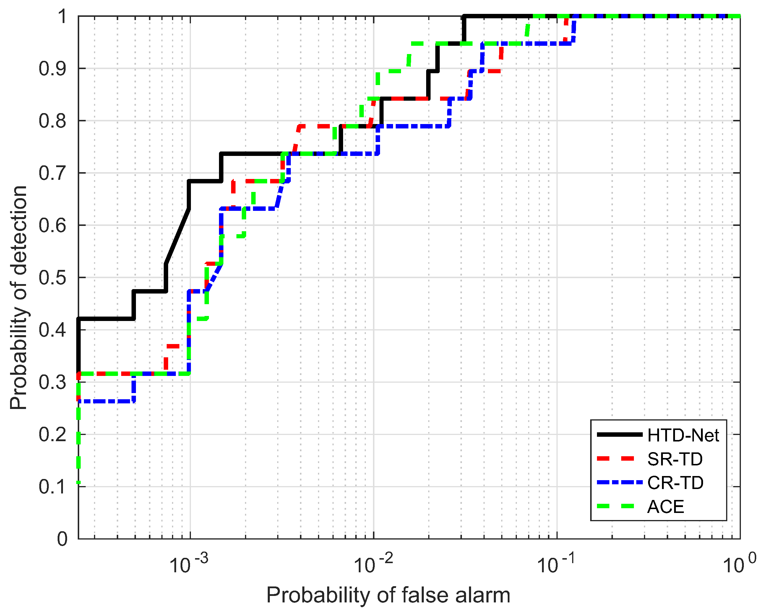
Figure 17.
ROC performance of the proposed method for the HyMap data.
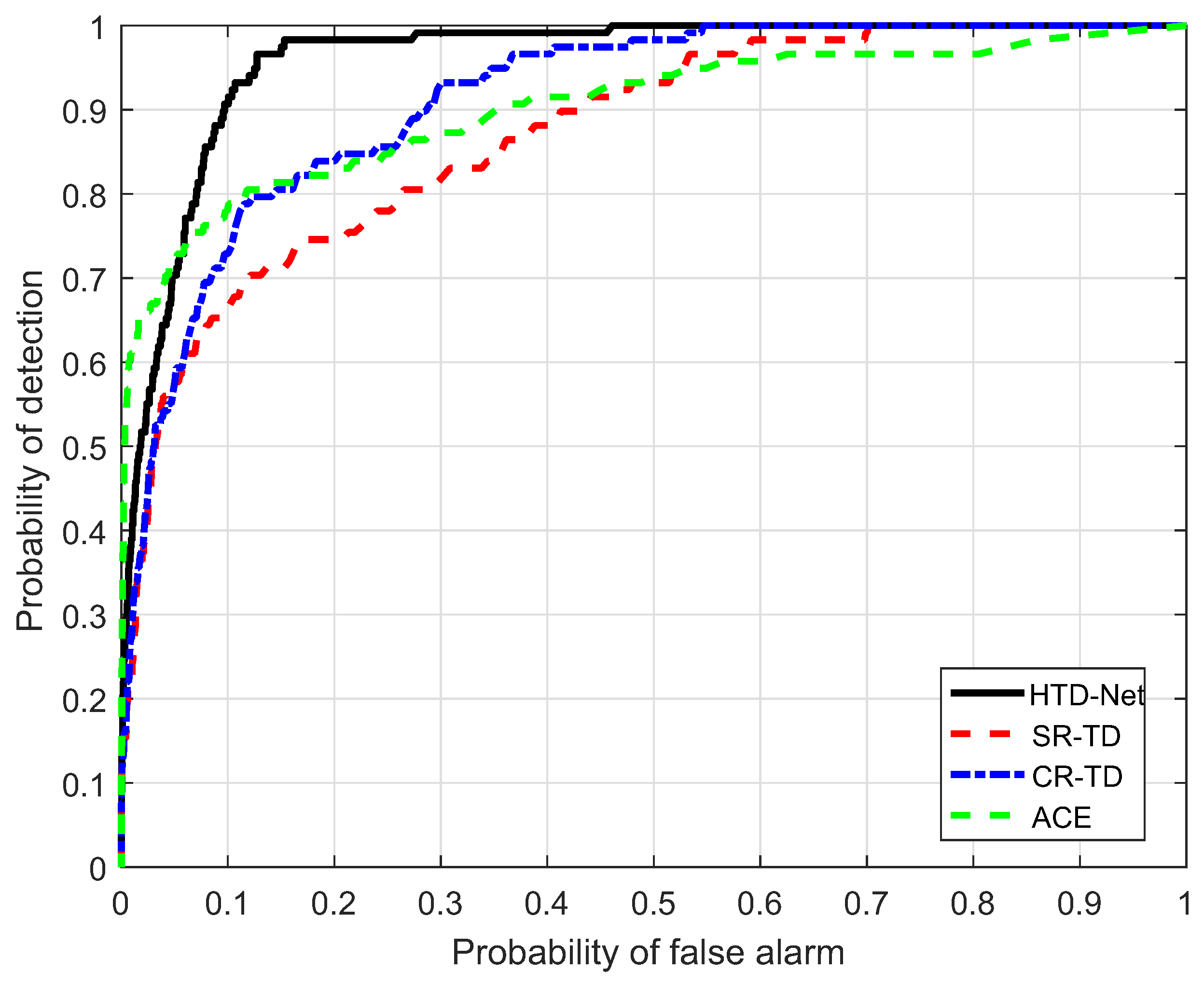
Figure 18.
Detection maps for the Moffett Filed image, is set to 0.0001. (a) adaptive coherence estimator (ACE): . (b) sparse representation-based target detector (SR-TD): . (c) collaborative representation-based target detection (CR-TD): . (d) HTD-Net: .
Figure 18.
Detection maps for the Moffett Filed image, is set to 0.0001. (a) adaptive coherence estimator (ACE): . (b) sparse representation-based target detector (SR-TD): . (c) collaborative representation-based target detection (CR-TD): . (d) HTD-Net: .
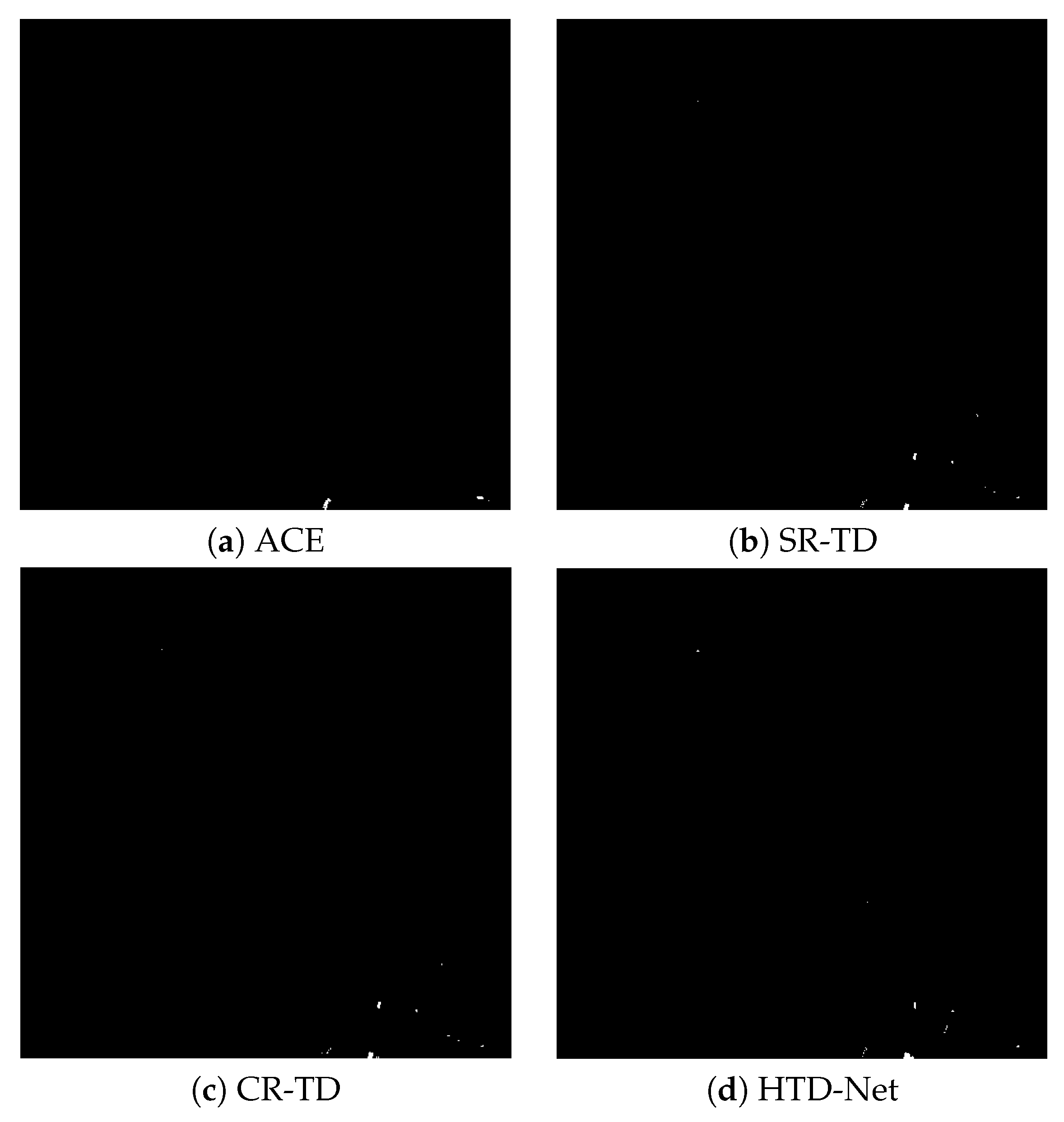
Figure 19.
Detection maps for the WTC image, is set to 0.003. (a) ACE: . (b) SR-TD: . (c) CR-TD: . (d) HTD-Net: .
Figure 19.
Detection maps for the WTC image, is set to 0.003. (a) ACE: . (b) SR-TD: . (c) CR-TD: . (d) HTD-Net: .
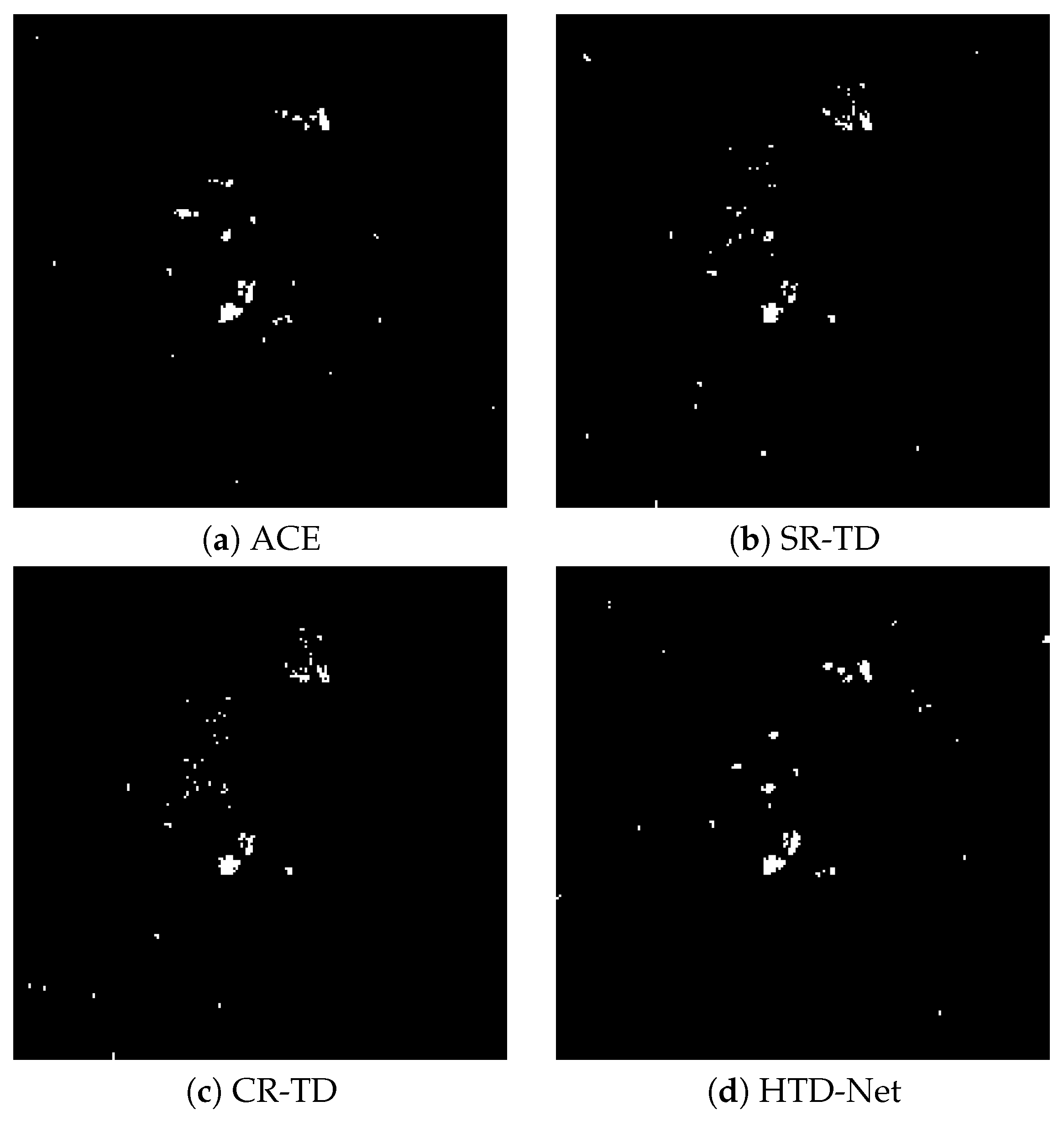
Figure 20.
Detection maps for the Hydice Forest image, is set to 0.002. (a) ACE: . (b) SR-TD: . (c) CR-TD: . (d) HTD-Net: .
Figure 20.
Detection maps for the Hydice Forest image, is set to 0.002. (a) ACE: . (b) SR-TD: . (c) CR-TD: . (d) HTD-Net: .


Table 1.
Area under the curve (AUC) performance (%) comparison of the two regression models for the four experimental data.
Table 1.
Area under the curve (AUC) performance (%) comparison of the two regression models for the four experimental data.
| Data | Model | Target Samples | Background Samples | Combined Samples |
|---|---|---|---|---|
| Moffett Filed | Logistic | 98.12 | 64.39 | 99.72 |
| Linear | 99.8 | 72.24 | 99.91 | |
| WTC | Logistic | 84.77 | 67.63 | 84.19 |
| Linear | 85.59 | 91.57 | 99.31 | |
| Hydice Forest | Logistic | 93.80 | 70.74 | 97.47 |
| Linear | 98.50 | 86.72 | 99.49 | |
| HyMap | Logistic | 72.64 | 70.60 | 80.47 |
| Linear | 95.34 | 90.27 | 96.03 |
Table 2.
AUC performance (%) comparison of the four detectors.
| Data | Detectors | |||
|---|---|---|---|---|
| ACE | CR-TD | SR-TD | HTD-Net | |
| Moffett Filed | 97.98 | 98.25 | 98.04 | 99.91 |
| WTC | 98.69 | 95.17 | 98.65 | 99.31 |
| Hydice Forest | 99.32 | 98.68 | 98.82 | 99.49 |
| HyMap | 90.29 | 91.29 | 87.20 | 96.03 |
Table 3.
Statistical significance of the difference between different detectors.
| HTD-Net | AUC (%) | Standard | Z | p | Significant? | Significant? |
|---|---|---|---|---|---|---|
| vs. | Difference | Error | Statistic | Value | (95% Confidence) | (99% Confidence) |
| Moffett Filed | ||||||
| ACE | 1.93 | 0.0026 | 7.415 | <0.0001 | Yes | Yes |
| CR-TD | 1.66 | 0.0022 | 7.533 | <0.0001 | Yes | Yes |
| SR-TD | 1.87 | 0.0025 | 7.471 | <0.0001 | Yes | Yes |
| WTC | ||||||
| ACE | 0.62 | 0.0016 | 3.873 | <0.0001 | Yes | Yes |
| CR-TD | 4.14 | 0.0049 | 8.345 | <0.0001 | Yes | Yes |
| SR-TD | 0.66 | 0.0017 | 3.908 | 0.0001 | Yes | Yes |
| Hydice Forest | ||||||
| ACE | 0.17 | 0.0023 | 0.745 | 0.745 | No | No |
| CR-TD | 0.81 | 0.0036 | 2.260 | 0.0238 | Yes | No |
| SR-TD | 0.67 | 0.0032 | 2.081 | 0.0375 | Yes | No |
| HyMap | ||||||
| ACE | 5.74 | 0.0089 | 6.410 | <0.0001 | Yes | Yes |
| CR-TD | 4.74 | 0.0082 | 5.760 | <0.0001 | Yes | Yes |
| SR-TD | 8.83 | 0.0110 | 8.023 | <0.0001 | Yes | Yes |
Table 4.
Comparison of the execution time of different detectors (in seconds).
| Data | Detectors | |||
|---|---|---|---|---|
| ACE | CR-TD | SR-TD | HTD-Net | |
| Moffett Filed | 4.68 | 10.38 | 15.53 | 83.33 |
| WTC | 0.71 | 1.83 | 2.49 | 58.35 |
| Hydice Forest | 0.05 | 0.17 | 0.21 | 2.23 |
| HyMap | 0.31 | 1.02 | 1.29 | 28.17 |
© 2020 by the authors. Licensee MDPI, Basel, Switzerland. This article is an open access article distributed under the terms and conditions of the Creative Commons Attribution (CC BY) license (http://creativecommons.org/licenses/by/4.0/).
Share and Cite
MDPI and ACS Style
Zhang, G.; Zhao, S.; Li, W.; Du, Q.; Ran, Q.; Tao, R. HTD-Net: A Deep Convolutional Neural Network for Target Detection in Hyperspectral Imagery. Remote Sens. 2020, 12, 1489. https://0-doi-org.brum.beds.ac.uk/10.3390/rs12091489
AMA Style
Zhang G, Zhao S, Li W, Du Q, Ran Q, Tao R. HTD-Net: A Deep Convolutional Neural Network for Target Detection in Hyperspectral Imagery. Remote Sensing. 2020; 12(9):1489. https://0-doi-org.brum.beds.ac.uk/10.3390/rs12091489
Chicago/Turabian StyleZhang, Gaigai, Shizhi Zhao, Wei Li, Qian Du, Qiong Ran, and Ran Tao. 2020. "HTD-Net: A Deep Convolutional Neural Network for Target Detection in Hyperspectral Imagery" Remote Sensing 12, no. 9: 1489. https://0-doi-org.brum.beds.ac.uk/10.3390/rs12091489
Note that from the first issue of 2016, this journal uses article numbers instead of page numbers. See further details here.