Monitoring the Vertical Land Motion of Tide Gauges and Its Impact on Relative Sea Level Changes in Korean Peninsula Using Sequential SBAS-InSAR Time-Series Analysis

Abstract

The relative sea-level changes from tide gauges in the Korean peninsula provide essential information to understand the regional and global mean sea-level changes. Several corrections to raw tide gauge records are required to account for coastal vertical land motion (VLM), regional and local coastal variability. However, due to the lack of in-situ measurements such as leveling data and the Global Navigation Satellite System (GNSS), making precise assessments of VLM at the tide gauges is still challenging. This study aims to address the above limitation to assess the VLM in the Korean tide gauges using the time-series Interferometric Synthetic Aperture Radar (InSAR) technique. For 10 tide gauges selected in the Korean peninsula, we applied the Stanford Method for Persistent Scatterers (StaMPS)—Small Baseline Subset (SBAS) method to C-band Sentinel-1 A/B Synthetic Aperture Radar (SAR) data acquired during 2014/10–2020/05, with the novel sequential interferograms pair selection approach to increase the slowly decorrelating filtered phase (SDFP) pixels density near the tide gauges. Our findings show that overall the tide gauges in the Korean peninsula are stable, besides the largest VLM observed at Pohang tide gauge station (East Sea) of about −26.02 mm/year; also, higher rates of uplift (>1 mm/year) were observed along the coast of Yellow Sea (Incheon TG and Boryeong TG) and higher rates of subsidence (<−2 mm/year) were observed at Jeju TG and Seogwipo TG. Our approach estimates the rate of VLM at selected tide gauges with an unprecedented spatial and temporal resolution and is applicable when the in-situ and GNSS observations are not available.

1. Introduction

The vulnerability of coastal areas due to sea-level rise inundation has received increasing attention in the years since the rise of the global mean sea level of about 11–16 cm in the 20th century [1]. Meanwhile, the sea level is forecasted to rise about 0.5 m to 2 m in the 21st century due to climate change that is driven by carbon emissions and Antarctica’s ice sheet instability [1,2,3]. Since the sea-level rise has direct impacts on small islands and low-lying coastal regions where immense growth of population is taking place, reliable sea-level projections are extremely important for mitigation planning from flooding and coastal erosion [4].

Global monitoring of oceans for sea-level changes is mainly accomplished by tide gauge records [5,6] and satellite altimetry estimates [7,8]. Since 1992, satellite radar altimetry has provided near-global measurements of sea surface height (SSH) with reference to geocentric frame [8,9]. Before the satellite altimetry, the network of tide gauges distributed on the world coasts and inland played a vital role in understanding sea-level changes [9]. Since 1901, tide gauges have provided long-term instrumental records of relative sea-level (RSL) with reference to local benchmarks [6,10]. Several approaches have been performed to reconstruct the global mean sea level (GMSL) using long-term RSL from tide gauge networks [6,9,11]. However, often the rate of RSL changes show inconsistency among the neighboring tide gauges. Tide gauges records in the coastal areas comprise global mean rise, regional variability, ocean processes, and local vertical land motions [12]. In particular, vertical land motion (VLM) in the vicinity of tide gauges and coastlines exacerbated the relative sea-level changes from tide gauge records, especially in the delta regions or basins which are vulnerable to rapid compaction of sediments [12,13]. In the context of global mean sea-level studies, the influence of local vertical land motion is an essential component that needs to be removed from tide gauge records for improved sea-level estimates [14,15]. Over the years, the number of permanent Global Navigation Satellite System (GNSS) was co-located at a tide gauge to provide high-quality estimates of vertical land motion [16,17]. VLM estimates from co-located GNSS stations were found to be acceptable supplemental information for sea-level estimates [16]. However, only 14% of tide gauge stations in the Global Sea Level Observing System (GLOSS) tide gauge stations are directly equipped with permanent GNSS stations [13,18].

On the other hand, the Interferometric Synthetic Aperture Radar (InSAR) technique is employed to estimate the ground motion at tide gauges for compensating the VLM component in the relative sea-level changes [14,19,20]. Time-series InSAR techniques utilize the Synthetic Aperture Radar (SAR) data to measure the differential ground motion of the earth’s surface during the period of acquisitions with a sub-millimeter level of accuracy [21,22]. Nonetheless, the retrieval of the deformation signal from time-series InSAR data is limited by several decorrelation factors including atmospheric delay, geometrical, temporal, orbital inaccuracies, and topographic errors [23,24]. To overcome this limitation, the persistent scatterers InSAR (PS-InSAR) [24,25] and small baseline subsets (SBAS) methods [26,27] have been introduced with recent advancements in time-series InSAR analysis such as SqueeSAR [28] and sequential estimator [29,30]. With the large archive of current generation SAR acquisitions such as Sentinel-1 A/B, Cosmo-SkyMed, and TerraSAR-X, multi-temporal InSAR analysis has gained further notice in monitoring the vertical ground motions over large areas [31]. It is worth noting that European Space Agency’s (ESAs) Sentinel-1 A/B constellation is a C-band SAR that has Interferometric Wide-swath (IW) acquisitions and high-revisit frequency enables the possibility of monitoring the targeted areas on a routine basis.

In this study, we focus on the 10 tide gauges that have exhibited abnormal sea-level trends in the last decade to assess the coastal vertical land motion at the precision of sub-millimeter per year. Until now, except for the Pohang tide gauge station, the relative sea-level changes were not corrected for vertical land motion. We, therefore, aim to investigate the vertical land motion (VLM) of tide gauges in the Korean Peninsula using the multi-temporal InSAR analysis as a representative exploration toward the open oceanic conditions and shallow seas. Additionally, our approach of using sequential-InSAR pair selection will complement the StaMPS-SBAS algorithm to address the question of increasing the initial slowly decorrelating filtered phase (SDFP) pixels density around the coastal region. For the first time, this study examines the capability of multi-track (ascending and descending mode) Sentinel-1 ground displacements for VLM estimates at multiple tide gauges over the entire coast of the Korean Peninsula. For this, we acquired sentinel-1 SAR data from six ascending and six descending frames over the study area, from October 2014 to May 2020. Section 2 presents a brief overview of the acquisition of SAR datasets and the relative sea-level changes from tide gauges and GPS data. A sequential pair selection-based approach to StaMPS-SBAS for estimating VLM at tide gauges using C-band Sentinel-1 A/B SAR data is presented in Section 3. Section 4 presents the experiment result of vertical land motions at each case study tide gauges. In Section 5 and Section 6, the results of vertical land motion at case study tide gauges are discussed and finally, the conclusions are summarized.

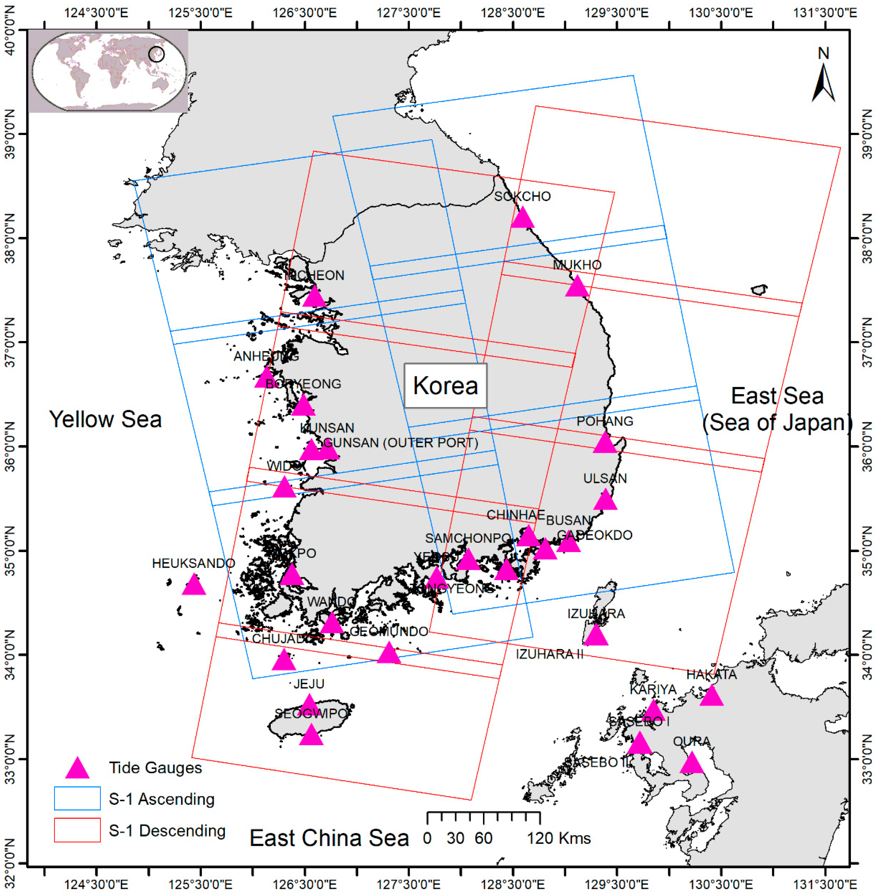
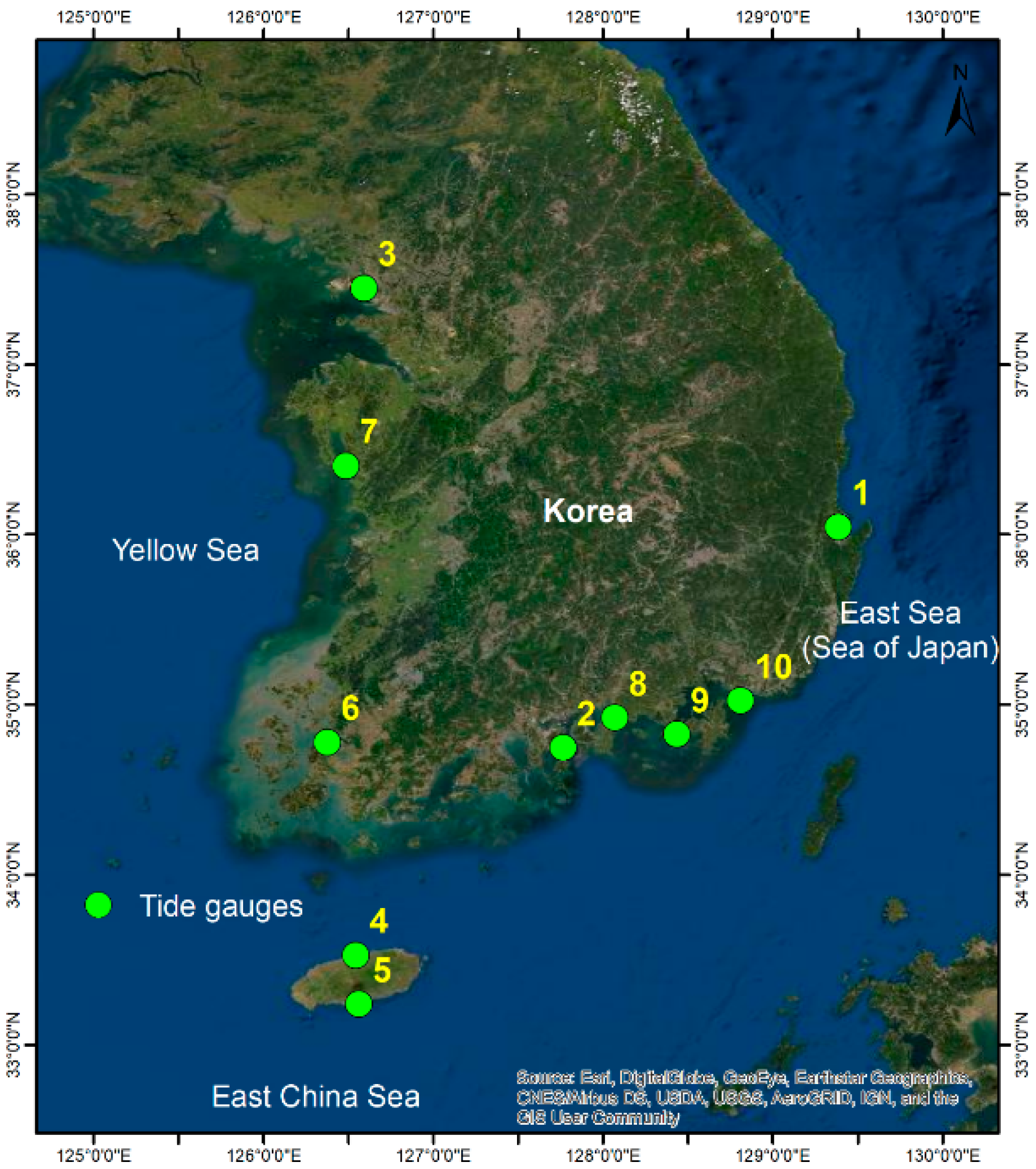
2. Study Area and Data Used

Here, we chose the Korean Peninsula as the case study area to estimate the VLM trend at tide gauges using multi-temporal Sentinel-1 SAR data. The Korean Peninsula is located in East Asia and is surrounded by the three marginal seas: East Sea/Japan Sea, East China Sea, and the Yellow Sea as shown in Figure 1. This coastal region was selected because the diverse and complicated hydrodynamic setting of these seas provides a unique opportunity to represent regional differences for understanding global changes. According to the Intergovernmental Panel on Climate Change (IPCC) report, the sea-level rise around the Korean peninsula is higher than the global mean sea-level trend [32]. The rate of sea-level rise in the East Sea is relatively higher than that in the Yellow Sea and the East China Sea, and sea-level rise for the East China Sea and Yellow Sea is similar. Based on the linear analysis of 19 tide gauge records around the Korean peninsula, the long-term relative sea-level changes were comparatively smaller along the western coast (~2.0 mm/year) than the eastern coast and around Jeju island (~3.6 mm/year and ~3.8 mm/year, respectively) [32]. The East/Japan Sea is one of the marginal seas on the northwestern pacific but it has subtropical and subarctic circulations bounded by a sub-arctic front similar to the open oceans. This East/Japan Sea has peculiar deep water called proper water and the upper portion of this water mass is produced by deep convection, which is also called open-ocean convection that is observed in the Mediterranean Sea and Antarctic Ocean. The Yellow Sea and the East China Sea are the semi-enclosed shallow marginal seas (average depth of 40 m) between China mainland and the Korean Peninsula that have been found to be warming steadily in the last century [32]. This warming trend of Sea Surface Temperature (SST) is more than the global mean SST, which eventually can cause sea-level rise and change in ocean currents.

2.1. Interferometric SAR Data

The Synthetic Aperture Radar (SAR) dataset over the Korean Peninsula was acquired by the C-band Sentinel-1 A/B satellite from October 2014 to May 2020. The acquisitions consisted of six frames each in ascending and descending mode (50 to 65 scenes for each frame). The number of acquisitions for each path and frame is shown in Figure 1. European Space Agency’s (ESA) Sentinel-1 A/B satellite has the IW acquisition mode, also referred to as Terrain Observation with Progressive Scans (TOPS) with a 6-day revisit time. Each IW scene comprised three sub-swaths that cover the area in the range of 250 km and the single-look spatial resolution for this dataset is 5 m in range and 20 m in azimuth.

2.2. Tide Gauge and GPS Data

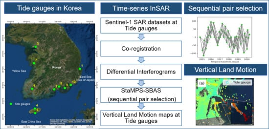
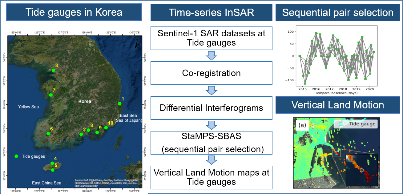
Monthly mean sea-level observation data for the tide gauges shown in Figure 2 were collected from KOOFS of Korean Hydrographic and Oceanographic Agency (KHOA) [33] http://www.khoa.go.kr/oceangrid/khoa/koofs.do). The hourly observed sea-level measurements at 21 tide gauge stations with long-term tidal records were acquired during 2009–2018 and processed to generate monthly data, then were provided to the Permanent Service for Mean Sea Level (PSMSL) [5]. We used the sea-level data from 10 stations as listed in

Table 1. Tide gauge stations used in the interferometric analysis.

S.No	Station Name	Latitude	Longitude
1.	Pohang	36.047222	129.383889
2.	Yeosu	34.747198	127.765873
3.	Incheon	37.451944	126.592222
4.	Jeju	33.5275	126.543056
5.	Seogwipo	33.24	126.561667
6.	Mokpo	34.779722	126.375556
7.	Boryeong	36.406389	126.486111
8.	Samchonpo	34.92416667	128.06972222
9.	Tongyeong	34.8275	128.434722
10.	Gadeokdo	35.025	128.811

. We calculated the long-term trend of sea-level change around the Korean coast based on the arithmetically averaging method, which combines the interpolated value of harmonic analysis [34]. The seasonal cycles of the tide gauge records were removed and a simple linear regression model was used to estimate the linear trend that represents the rate of sea-level rise [35]. The rate of sea-level rise was calculated for a period of 10 years (2009–2018) as shown in supplemental Figure S1. We collected the GPS observation from the co-located GPS station equipped with tidal stations, which were provided by KHOA.

3. Methods

For the multi-temporal InSAR analysis, we employed the StaMPS-Small Baseline Subset (StaMPS-SBAS) time-series analysis of single-look slowly-decorrelating filtered phase (SDFP) pixels in a single-look interferograms [27,36,37]. StaMPS-SBAS has the ability to identify the isolated SDFP pixels surrounded by completely decorrelated pixels. Whereas the standard SBAS methods process with interferograms that are multi-looked, filtered, and unwrapped the phase individually [26]. Additionally, a statistical cost flow 3D phase unwrapping (space and time) algorithm is applied to unwrapping the phase of SDFP pixels in the time-series multiple master interferograms [38].

Fundamentally, a network of multiple master interferograms is constructed based on small baseline methods that have minimized perpendicular, temporal, and Doppler baselines to reduce the decorrelation effects due to geometrical, temporal, and topographic errors. Further, spectral filtering in the range is applied to reduce the phase decorrelation and discard the non-overlapping Doppler frequencies in azimuth [27,39].

StaMPS-SBAS method uses the amplitude difference dispersion index ($D_{∆,A}$) as the proxy for detecting the initial subset of SDFP pixels candidates through the analysis of amplitudes, to reduce the computational burden. The amplitude difference dispersion index (as stated in Equation (1)), which is similar to the amplitude dispersion index $D_A$, is considered a better indicator for the phase stability when spectral filtering is applied in range [27].

$$D_{∆,A}=\frac{{\sigma }_{∆A}}{{\mu }_A}=\frac{\sqrt{\frac{{\sum }_{i=1}^N{(\left|M_i\right|-\left|S_i\right|)}^2}{N}}}{\frac{1}{2N}{\sum }_{i=1}^N\left|s_i\right|},$$

(1)

where,${\sigma }_{∆A}$ is the standard deviation of the difference in amplitude between master and slave, and $s_i$ is the amplitude of the pixel in the ith image, and N is the number of images. The simple thresholding of Amplitude Dispersion Index (ADI) $D_A$ is used to select the point scatterers i.e., PS pixels [25]; however, $D_{∆,A}$ is a better estimate of SDFP pixels [27]. In this method, the pixels having the lower $D_{∆,A}$ value than the commonly used threshold value ($D_{∆,A}$ < 0.6) are selected as initial PS candidates for selecting SDFP pixels.

Following that, a phase stability analysis is performed for each selected SDFP candidate by subtracting the spatially correlated and spatially uncorrelated components. Eventually, the final SDFP pixels are selected among the candidates by estimating the temporal coherence (${\gamma }_x)$ as proposed by [38],

$${\gamma }_x= \frac{1}{N} \left|{\sum }_{i=1}^N{e}^{j\left({\phi }_{x,i}-{\overline{\phi }}_{x,i}- ∆\widehat{\phi }\begin{array}{c}u\\ x,i\end{array}\right)}\right|,$$

(2)

where N is the number of interferograms, ${\phi }_{x,i}$ is the differential interferometric phase of x pixel in the ith interferogram.${\overline{\phi }}_{x,i}$ is the spatially correlated terms including deformation, atmospheric contribution, orbital error, and spatially correlated topographic phase due to DEM error which are computed iteratively using a combined low pass and adaptive phase filters. $∆\widehat{\phi }\begin{array}{c}u\\ x,i\end{array}$ is the spatially uncorrelated part of the topographic phase that correlates with perpendicular baseline. Finally, the PS points are selected from PS candidates by considering their amplitude dispersion value and temporal coherence. A threshold on gamma as a function of dispersion index and the percentage density of random (non-PS) pixels is set using the probability function.

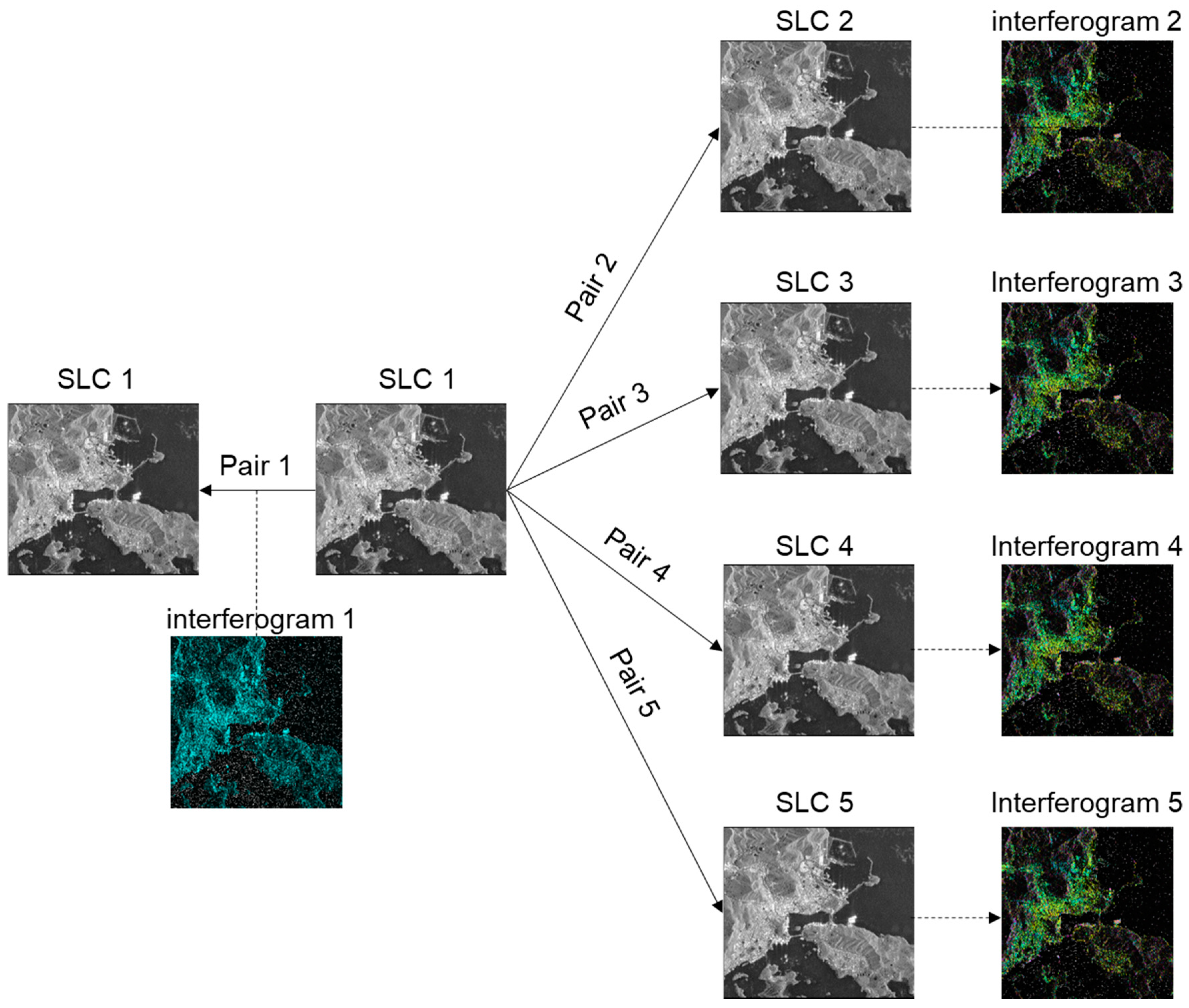
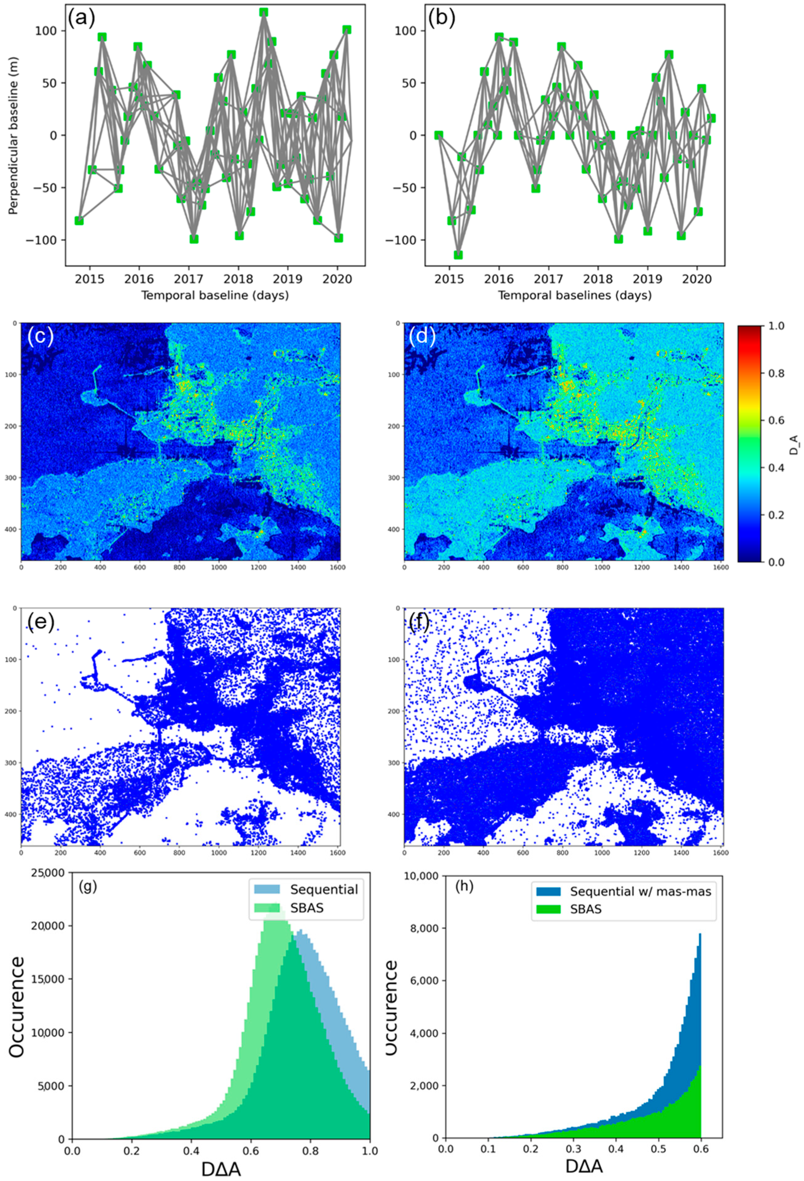
3.1. Sequential Pair Selection

In this study, a modified approach for the selection of interferograms is proposed to extend the amplitude difference dispersion index and optimize its measure to increase the density of SDFP candidates. To minimize the $D_{∆,A}$ criterion, we form the time-series interferograms in the sequential order (n = 5) for the StaMPS-SBAS algorithm, rather than standard StaMPS small baseline interferograms as shown in Figure S2. The approach is referred to as sequential InSAR pair selection for StaMPS-SBAS. In this study, M SAR images are assumed to be connected to N interferograms and N = (M × n) − n under the condition of n = 5 sequential SAR scenes. For SAR scene 1, the n interferograms are formed; this includes master–master interferograms as shown in Figure 3. We then apply temporal coherence ${\gamma }_x$ (Equation (2)) to identify the SDFP pixels. The main objective of this approach is to minimize the $D_{∆,A}$value of a pixel according to the Equation (1). To demonstrate the efficiency of this sequential pair selection approach, we conduct the comparative study using standard SBAS pair selection and sequential pair selection for StaMPS-SBAS as described in Section 3.1.1.

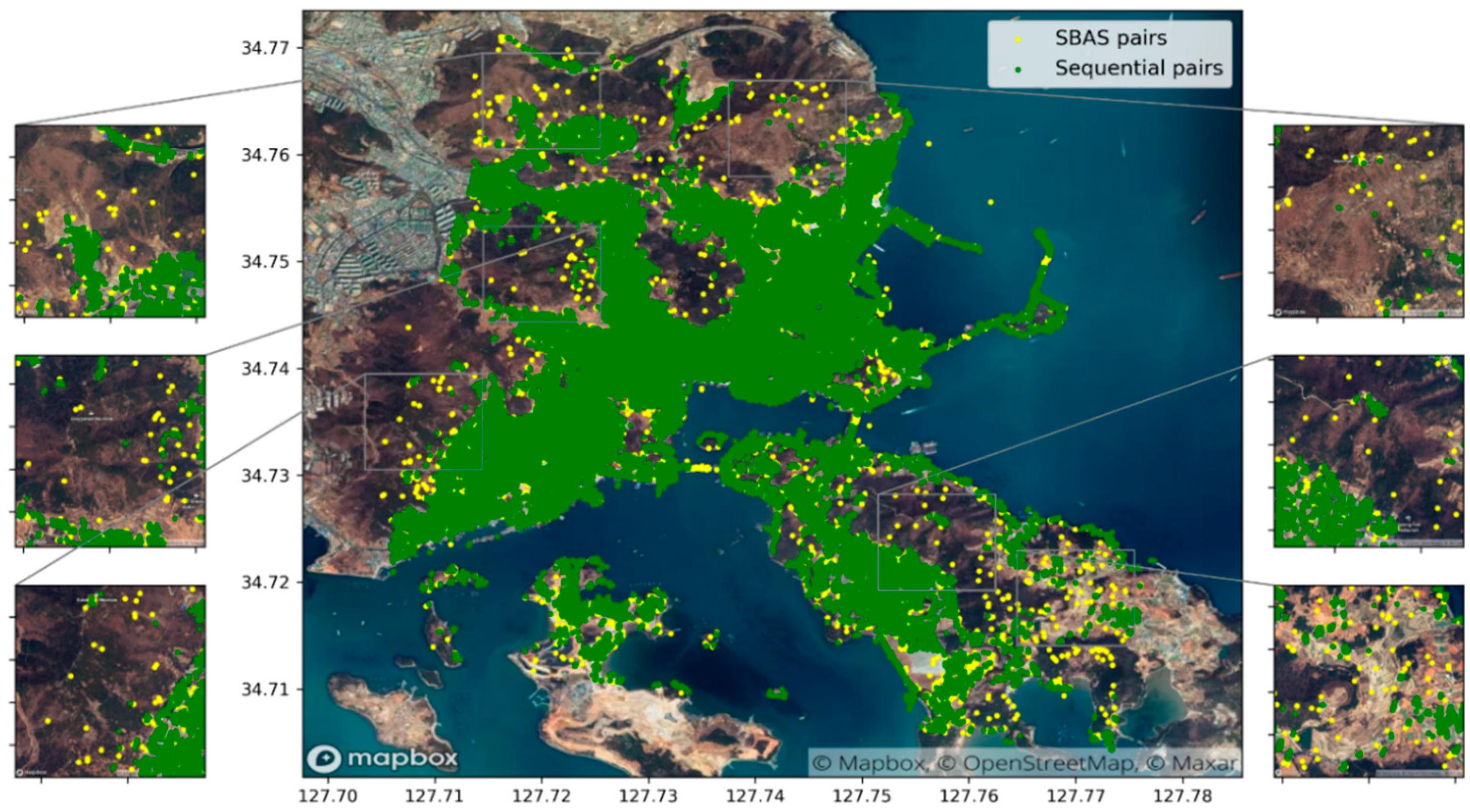
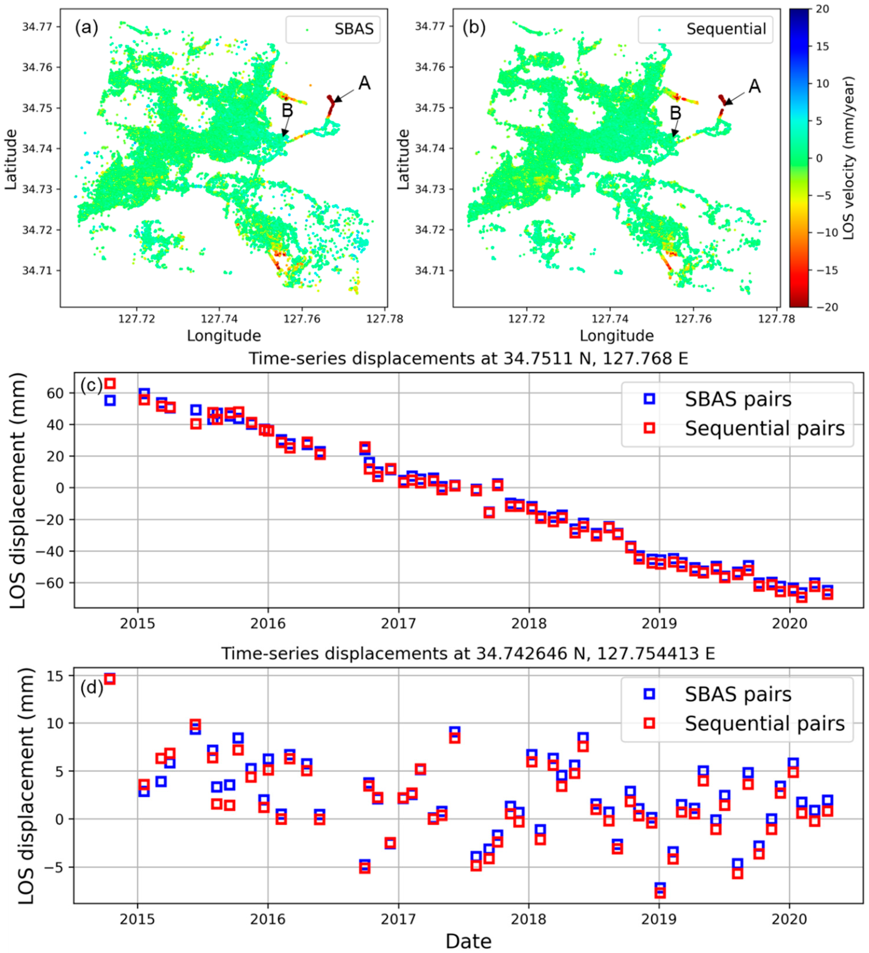
3.1.1. Experimental Results

To evaluate the approach, we applied the sequential pair selection in the StaMPS-SBAS algorithm as outlined in the previous section to the Yeosu region, located in the southern part of the Korean Peninsula. In this method, we processed 60 scenes of Sentinel-1 A/B single-look complex (SLC) scenes acquired during November 2014 and April 2019 in the descending mode. The TOPS stack Sentinel processor was implemented in this study using InSAR Scientific Computing Environment (ISCE) software [21,40,41] to generate a stack of co-registered SLC images and was resampled with respect to a master acquisition (the first scene in the acquisition). Sentinel-1 Precise orbit data and 1-arc second Digital Elevation Model (DEM) from Shuttle Radar Topography Mission (SRTM) were used in this processing to remove the topographic phase. To preserve the high-resolution phase information, we skipped the multi-looking step. Next, we generated a network of single-look interferograms for the subset area (1614 × 461 pixels) based on two cases (1) Standard StaMPS-SBAS pairs and (2) Sequential pair selection, n = 5 as described in Section 3.1. For the standard SBAS approach, we form the interferogram pairs with the thresholds of perpendicular baseline (Bperp) < ±250 m and temporal baseline (Btemp) < 250 days, which generates about 194 interferograms. On the other hand, for a sequential network, we form the interferograms with nearest neighbor images of 5 connections. This includes master–master, master–slave1, master–slave2, master–slave3 and master–slave4, which generates 290 interferograms (Figure 4). The parameters used for StaMPS-based SBAS InSAR processing are shown in supplemental Table S1. As shown in Figure 4, by applying the proposed approach the histogram of $D_{∆,A}$ values in sequential pair selection approach are skewed to the lower values of $D_{∆,A}$ compared to standard SBAS. By applying the thresholding value $D_{∆,A}$ less than 0.6, more SDFP candidates that have low amplitude pixels are selected in the sequential pair selection compared to standard SBAS pair selection.

Subsequently, SDFP pixels are selected based on both ${\gamma }_x$ and $D_{∆,A}$ values, having a minimum $D_{∆,A}$ and maximum ${\gamma }_x$ value fixed as the threshold [27]. The comparison of $D_{∆,A}$ and ${\gamma }_x$ of selected SDFP pixels between two approaches are shown in Figure S3. The total number of SDFP candidates for sequential pair selection is ~2 times as much as the standard SBAS pair selection. Considering the final selection of SDFP pixels for the sequential approach the number increased by ~1.2 times in comparison to the standard SBAS pair selection as illustrated in

Table 2. Comparison of slowly decorrelating filtered phase (SDFP) pixels statistics between StaMPS-SBAS and sequential pair selection approach.

S.No.	Description	StaMPS-SBAS	Sequential StaMPS-SBAS
1.	Initial SDFP selected candidates	60,731	124,467
2.	SDFP density (pixels/km2)	1230	2520
3.	Initial gamma threshold	0.3	0.3
4.	Re-estimated gamma threshold	0.002	0.265
5.	Selected SDFP pixels	55,515	66,792

.

Since the $D_{∆,A}$ value of almost every pixel is reduced to its minimum value by incorporating the master–master interferograms to the stack, the selection of SDFP pixel density was increased significantly (Figure 4). Eventually, this included SDFP pixel candidates over water regions that have low-amplitude pixels. In comparison to the SDFP candidates with standard StaMPS-SBAS, there is an improvement in the density of SDFP pixels over the port areas as shown in Figure 4e,f. Similarly, more numerous SDFP candidates were identified in the non-urban regions in the sequential pair selection approach.

As described in Table 2, the sequential pair selection approach selects about 1.2 times more SDFP pixels than the standard SBAS approach. Figure 5 illustrates the selected SDFP pixels overlaid on the OpenStreetMap© image. It is clearly shown that both approaches detect SDFP pixels commonly in the urban regions. However, taking a closer look at the zoomed inset images in Figure 5 shows that numerous SDFP pixels over the vegetation areas were retained in the standard SBAS approach, which could be false alarms, whereas our approach has the capability to drop SDFP pixels over dense vegetation and increased ~1.2 times the amount of SDFP pixels in the coastal areas, especially along the coasts.

Lastly, the comparison of mean velocity from the experimental results is presented in Figure 6. In a larger view, the major deformation signals exist in both approaches. It is worth noting that the line-of-sight (LOS) displacements in the final mean velocity maps comprise a considerable amount of noisy SDFP pixels in the standard StaMPS-SBAS, whereas in the sequential StaMPS-SBAS those noisy SDFP pixels were dropped in the spatially uncorrelated error estimation and phase stability analysis. Figure 6 shows that the time-series results derived from the sequential pair selection approach are quite consistent with standard StaMPS-SBAS. The time-series LOS displacements of pixel A, which is located in the significant ground motion region (Figure 6c) and pixel B, located in the slow deformation region (Figure 6d), reveal that the LOS displacements from the two approaches are consistent as well.

3.2. Experimental Setup

Based on the time-series interferometric analysis described in Section 3.1, we performed the StaMPS-SBAS analysis on the selected 10 tide gauge sites in the Korean Peninsula. The station information is listed in Table 1. Since this study aims to monitor the local ground motion at tide gauges and to reduce the computational time, we only processed the ground area that covers the tide gauge station and its vicinity rather than processing the entire scene, approximately about 0.04° × 0.04° size on the ground in the range and azimuth direction, respectively. The processing workflow for each station that is applied in this section is summarized in

Table 3. Processing workflow of StaMPS-SBAS for vertical land motion at each tide gauge.

Step	Processing Step	Product Output
1.	Acquisition of Sentinel-1 SAR data for each tide gauge station	SLCs stack for ascending and descending
2.	ISCE TOPS stack processor	Co-registered SLC stack, N
3.	Sequential pair selection (Section 3.1)	M sequential interferograms
4.	ISCE2StaMPS	Initial SDFP candidates
5.	StaMPS time-series analysis	Mean LOS velocity and time-series displacements
6.	LOS2VH decomposition	Vertical and horizontal velocity and time-series displacements

.

3.3. Vertical Land Motion

Using sequentially selected interferograms pairs in StaMPS-SBAS analysis, we estimated the one-dimensional (1D) mean velocity of SDFP pixels along the LOS direction for each SAR dataset (S1 ascending and S1 descending). As described in Equation (3), the mean LOS velocity results from ascending and descending datasets were combined to decompose the two-dimensional (2D) displacement vectors [19]. The 2D decomposition results provide the vertical (upward-downward) and horizontal (east-west) components over the overlapping acquisition date ranges and spatial coverage of viewing geometries.

$$\left[\begin{array}{c}{d}_{asc}\\ d_{desc}\end{array}\right]= \left[\begin{array}{cc}\cos {\theta }_{asc}& -\cos {\alpha }_{asc}\sin {\theta }_{asc}\\ \cos {\theta }_{desc}& -\cos {\alpha }_{desc}\sin {\theta }_{desc}\end{array}\right] \left[\begin{array}{c}{d}_{vert}\\ d_{hor}\end{array}\right],$$

(3)

4. Results

4.1. Vertical Land Motion at Tide Gauges in the Korean Peninsula

In this section, we present the results that were processed using the sequential pair selection for the StaMPS-SBAS approach as presented in Section 3.1. We present the processing results that resulted when we applied this method to 10 selected tide gauges stations around the coast of the Korean Peninsula as listed in Table 1. In this section, we present the mean vertical displacement rate of the selected tide gauge stations processed using StaMPS-SBAS with sequential interferogram pairs during the 2016–2020 SAR periods. The mean displacement rate map is superimposed on the satellite style base map from Mapbox.

We were able to acquire both ascending and descending track SAR data for 10 selected tide gauges; however, there is only descending track SAR data for 2 tide gauge stations (i.e., Jeju and Seogwipo). In the following sub-sections, the mean velocities and time-series InSAR displacements are presented for 5 tide gauges that showed significant sea-level change variations in the recent decade, namely, Pohang, Yeosu, Incheon, Jeju, and Seogwipo. The InSAR results for the remaining tide gauges are presented in the supplementary material (Figures S4–S8). The positive values in the mean velocity map indicate that the surface is uplifting, whereas the negative values indicate the subsidence in the vertical direction. The presented mean displacement rates map shows high-resolution InSAR derived ground motion at tide gauges and its vicinity. Since the spatial coverage of InSAR results in a small and adequate number of SAR scenes, the mean velocity maps are not affected by atmospheric noise or by orbital errors and ensure the reliability of the InSAR displacements.

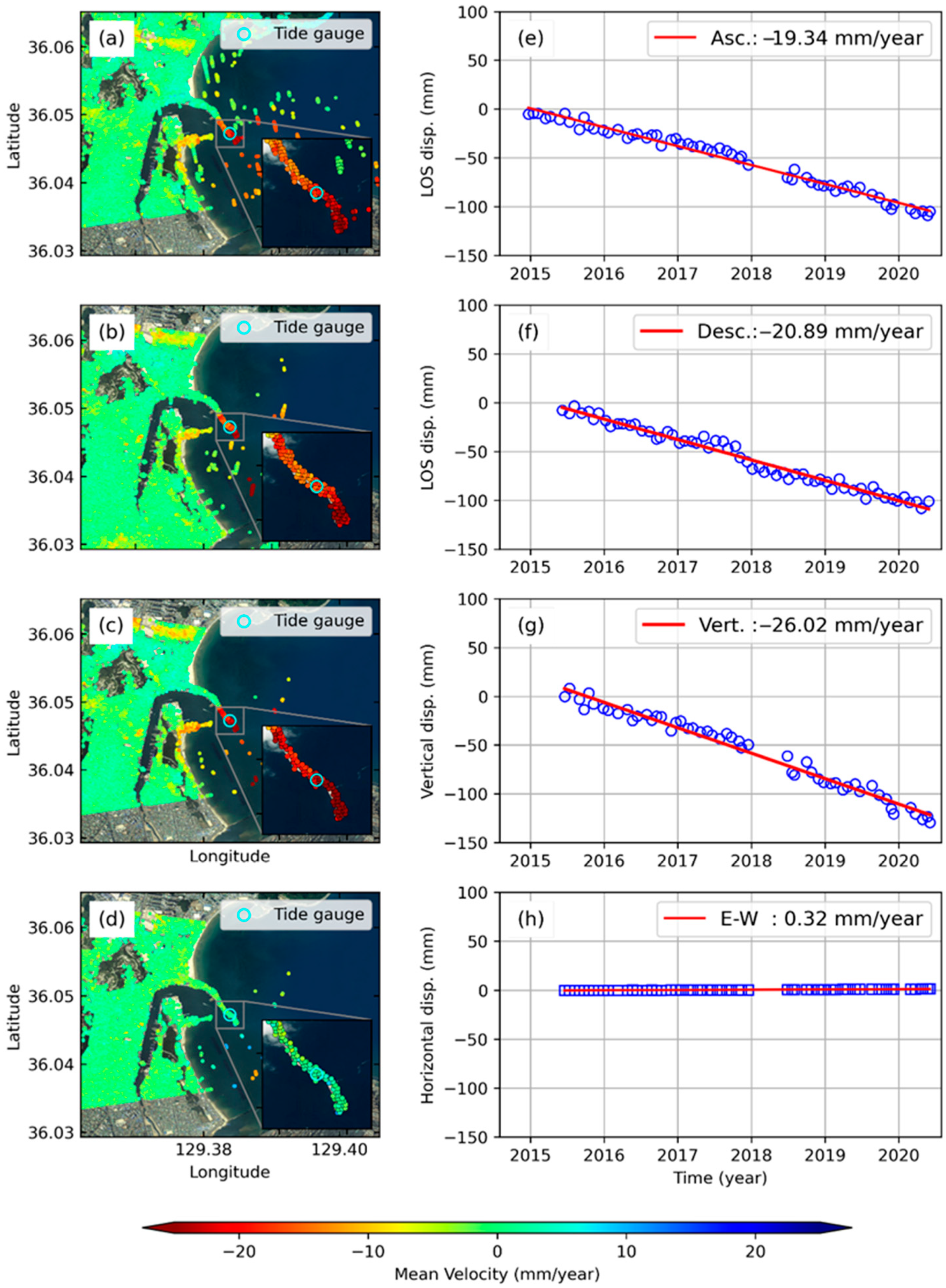
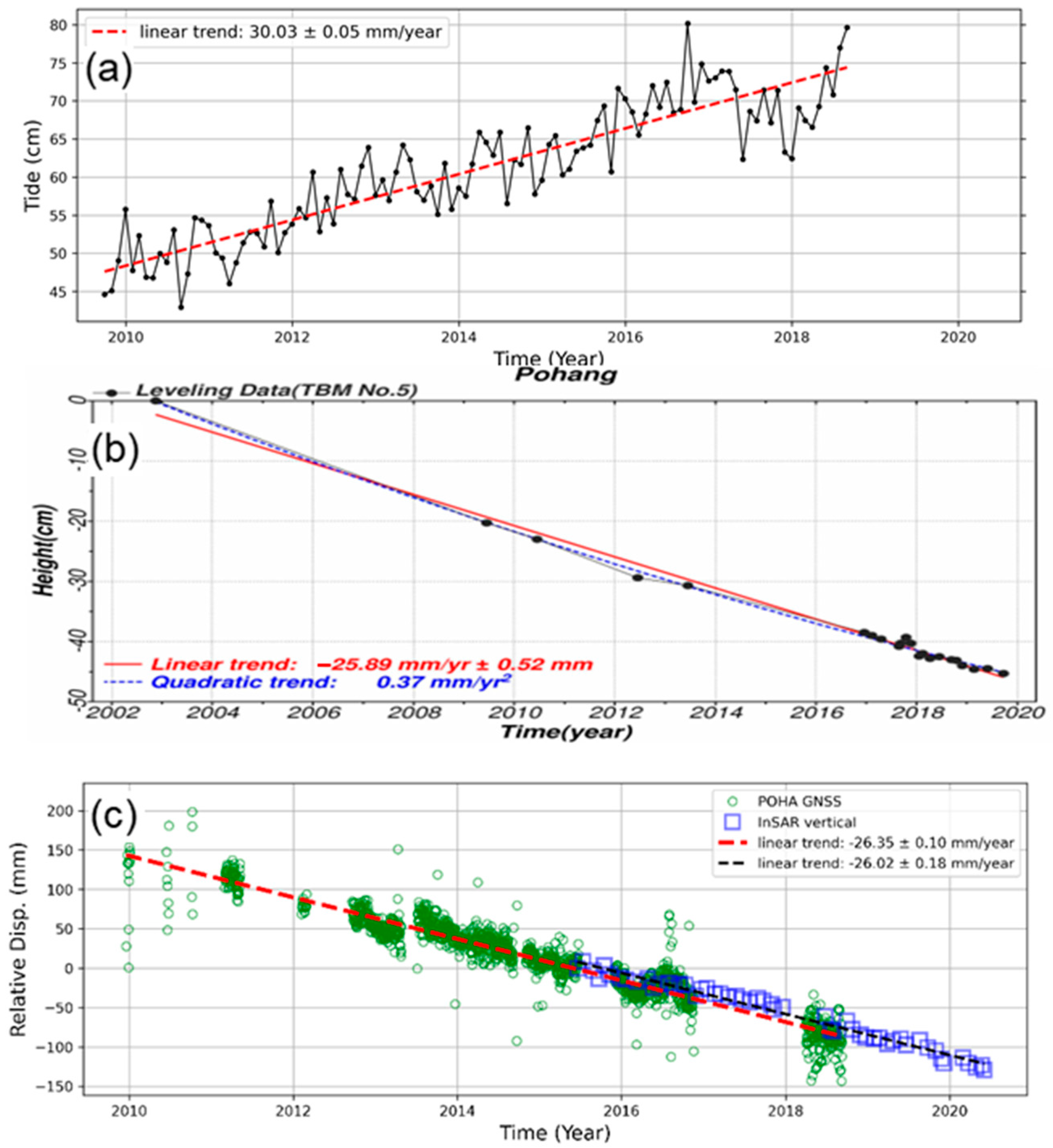
4.1.1. Pohang Tide Gauge

Pohang tide gauge station is located in the southeast of the Korean Peninsula on the coast of the East Sea. Figure 7 shows the spatial distribution of vertical ground motion at Pohang tide gauge, which was observed as significant sea-level changes in recent years. The Pohang tide gauge is situated on the breakwater as shown in Figure 7. For the first time, [19] reported the linear vertical land motion of the Pohang tide gauge using StaMPS PS-InSAR analysis and we applied the sequential pair selection for StaMPS-SBAS with additional recent datasets and observed continuous linear ground motion at the tide gauge station. The velocity maps reveal the linear displacement rates in the Pohang tide gauge station, about −19.34 mm/year, and −20.89 mm/year for ascending and descending track, respectively. On the other hand, the ground motion is quite stable in the inland areas. The InSAR derived vertical velocity was estimated at −26.02 mm/year and horizontal velocity along E–W direction as ±0.32 mm/year (Figure 7).

The relative sea-level changes obtained over the past 10 years (2010–2019) at the Pohang tide gauge station are illustrated in Figure 8a–c. The temporal variability of sea-level rise at Pohang TG is highlighted with decadal analysis. The Pohang TG has recorded the highest sea-level change fluctuation in the Korean Peninsula. Over the last 30 years, the sea-level rise at Pohang TG has significantly accelerated, and more importantly in the recent decade, the sea-level rise is estimated at 30.03 mm/year ± 0.05 mm, which is double the global mean sea-level rise value [42]. On the other hand, a permanent GNSS station co-located with Pohang TG has been available from 2010 to 2020. Some discontinuities in the time-series observation notwithstanding, the linear velocity is observed over the observation period.

By considering, the long-term sea-level trend obtained from tide gauge records, the tide gauge exhibits significant sea-level rise since the Pohang TG was relocated to the current location in the year 2002 [43] (https://www.gloss-sealevel.org/sites/gloss/files/publications/documents/Korea-National-Report-2019.pdf, last accessed on 18 September 2020). Since then, a linear increase in the sea-level rise was observed; therefore, KHOA applied de-trending for VLM using the leveling data observed about −25.89 mm/year (Figure 8b). It is worth noting that the vertical land motion derived from our SBAS-InSAR, co-located GNSS (Figure 8c), and leveling measurements are highly consistent with each other.

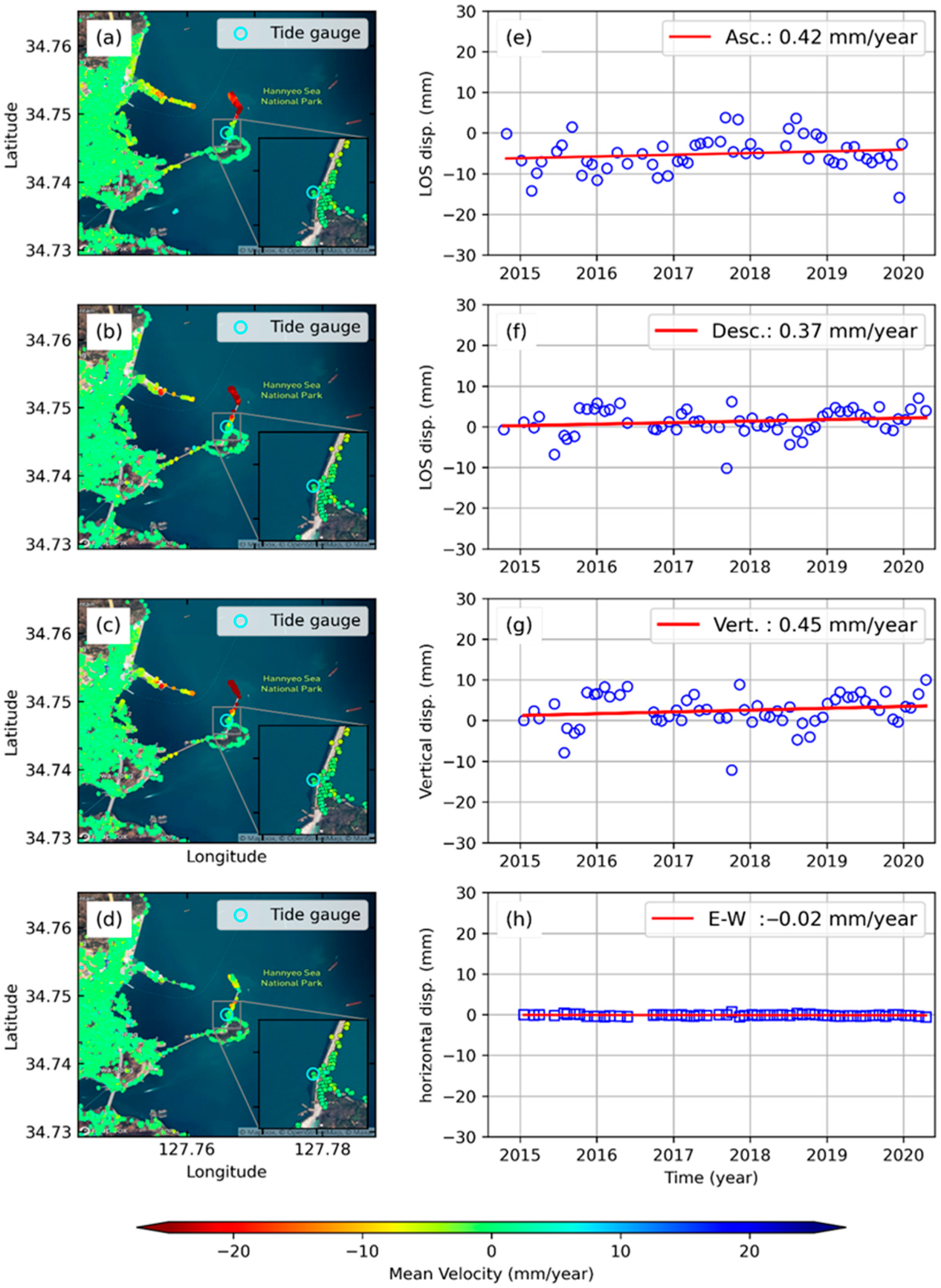
4.1.2. Yeosu Tide Gauge

Figure 9 illustrates the mean velocity maps and time-series displacements over the Yeosu tide gauge region located in the south of the Korean Peninsula on the coast of the East China Sea. Yeosu tide gauge is situated on the structure constructed on Odongdo island precisely on the point where the island meets breakwater. Most of the Yeosu region showed a fairly stable displacement rate, whereas the breakwater showed significant subsidence. However, the InSAR derived displacement rate at Yeosu TG showed slight uplift of about 0.45 mm/year (Figure 9). The time-series displacements reveal slight non-linear velocity at Yeosu TG (Figure 9g).

The Yeosu TG was chosen for demonstrating the effectiveness of sequential pair selection for StaMPS-SBAS analysis as described in Section 3. The relatively higher SDFP pixel density than ordinary StaMPS-SBAS, obtained using our approach showed the variation of displacement rate at high-resolution.

In contrast with Pohang TG, the monthly sea-level changes at Yeosu TG showed slight variability in sea-level rise over the 10 years between 2009 and 2018 (Figure S1). In the recent decade, the rate of sea-level change is estimated at 1.34 mm/year ± 1.29 mm, which is lower than the global mean sea-level rise. With no permanent GPS station and in-situ leveling data at Yeosu TG, the InSAR derived estimates provide the VLM estimates.

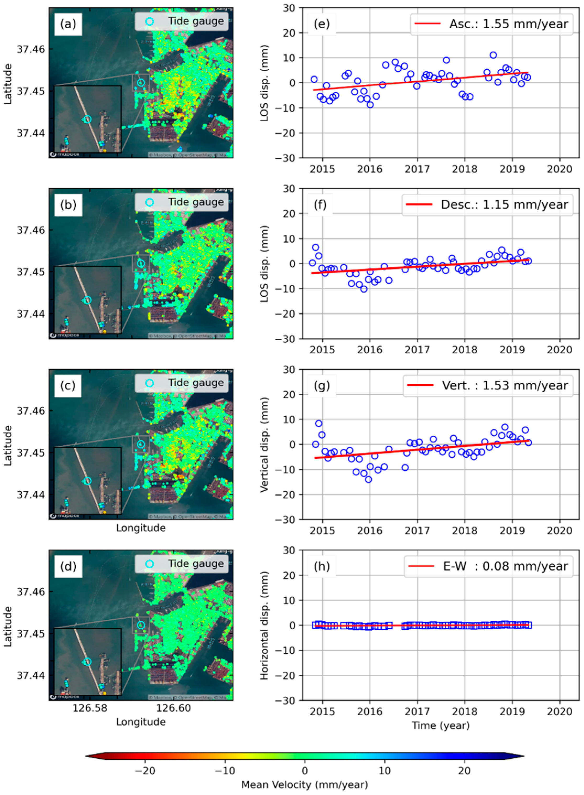
4.1.3. Incheon Tide Gauge

The Incheon tide gauge station is located in the west of the Korean Peninsula on the coast of the Yellow Sea. The tide gauge station is precisely located on the jetty at the port of Incheon. Figure 10 illustrates the InSAR derived mean velocity maps and time-series displacements estimated at Incheon TG. The StaMPS-SBAS analysis reveals the uplift in the LOS direction of about 1.55 mm/year and 1.15 mm/year in the ascending and descending track, respectively. The vertical land motion estimated at Incheon TG is +1.53 mm/year and 0.08 mm/year (E–W). The west coast of the Korean Peninsula has a vast tidal flat that was produced by high tidal amplitude [44]. The entire coastal harbor including Incheon TG is built on the reclaimed land.

Figure S1 shows the temporal variability of the sea-level change in the Incheon TG station. It is worth mentioning that the linear trend of sea-level change has been decreasing in recent years. The linear rate of sea-level change was lowered to 2.12 mm/year ± 1.23 mm during 2009–2018. The nearest GPS station is located approximately 31.5 km away from Incheon TG; therefore, it will not represent the local land motion directly at the tide gauge.

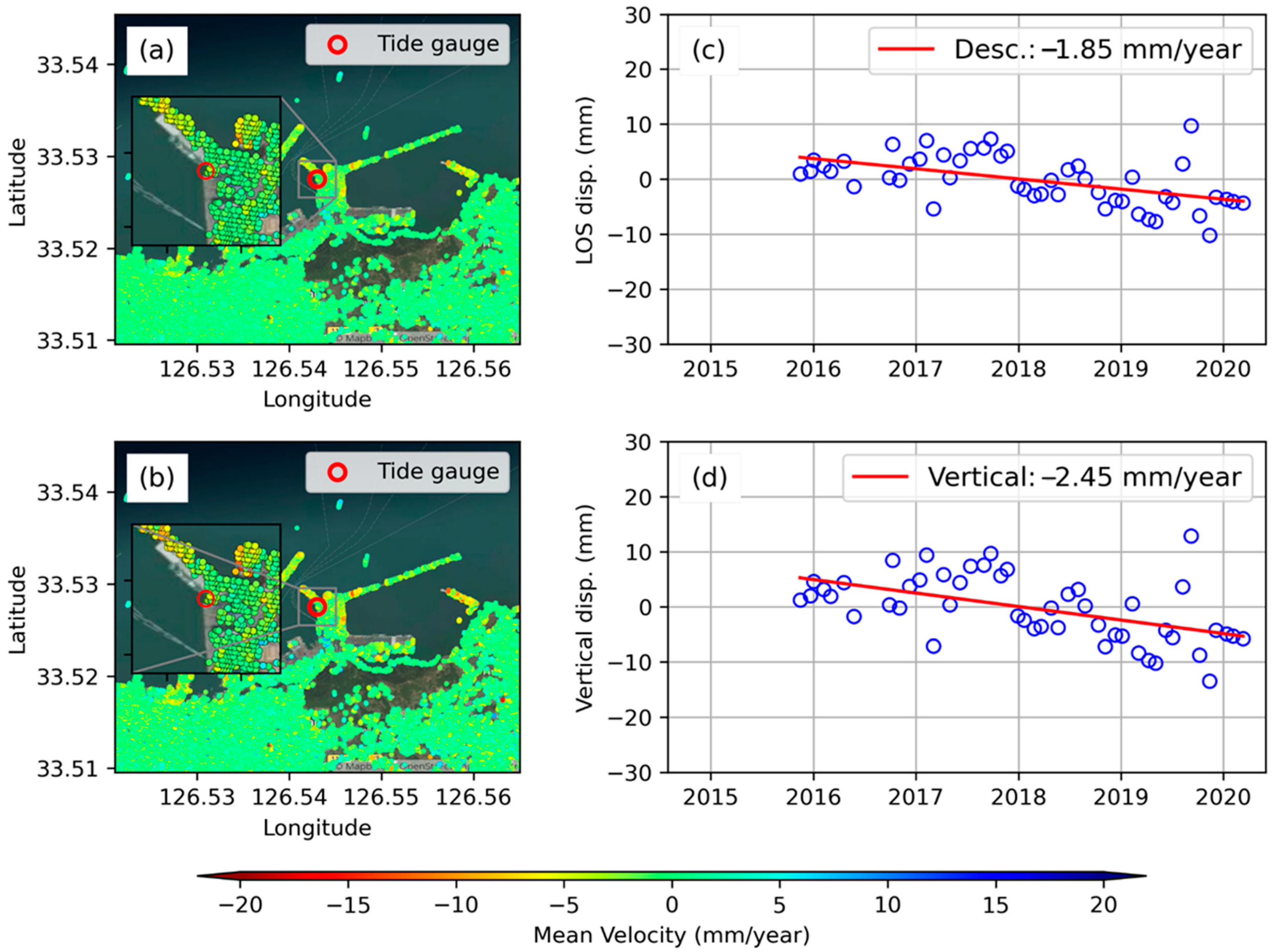
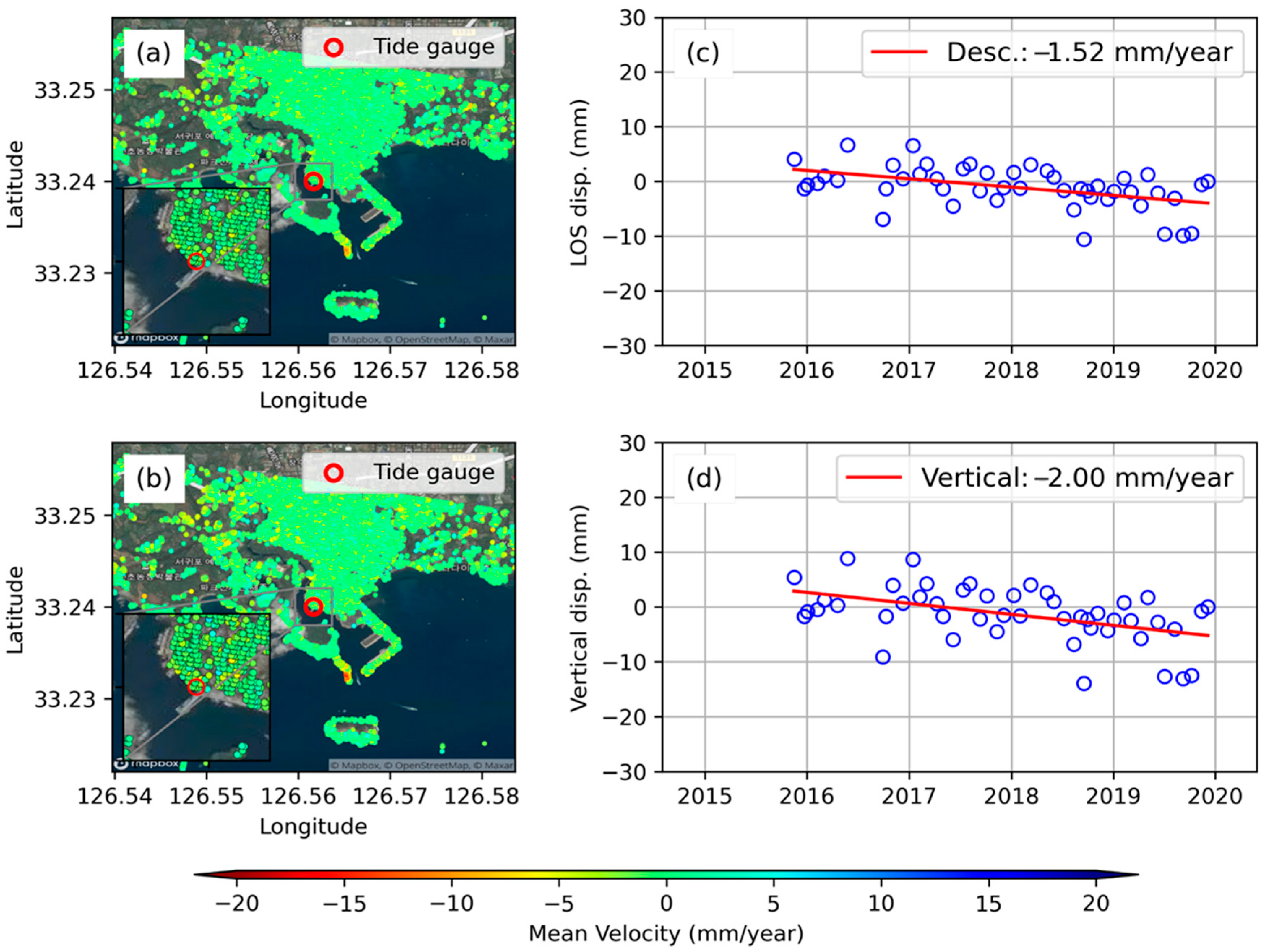
4.1.4. Jeju and Seogwipo Tide Gauges

Figure 11 and Figure 12 show the mean velocity maps and time-series displacements for Jeju TG and Seogwipo TG. These two stations are located on Jeju island, south of the Korean Peninsula. As mentioned in Section 2.1, we acquired Sentinel-1 data over Jeju island in descending mode only (ascending mode was not available). Therefore, it is not possible to estimate vertical and horizontal displacements as described in Section 3.3. However, we estimated the vertical displacement by dividing the LOS displacement by the cosine of the SAR incidence angle by ignoring the contribution of the horizontal component to LOS displacement [45]. The mean velocity maps reveal −2.45 mm/year and −2.0 mm/year displacement rate at Jeju TG and Seogwipo TG, respectively. For sea-level related studies, the common assumption is the VLM generally occurs in a near-linear trend. The linear downward ground motion trend in Seogwipo TG correlates with the sea-level rise observed in the last decade (Figure S1).

5. Discussion

We presented in this work a simple approach by sequential pair selection for estimating the vertical land motion of tide gauges selected in the Korean Peninsula using StaMPS-SBAS. Our experimental results demonstrate that incorporating the sequential pair selection with master–master interferograms minimizes the amplitude dispersion criterion and therefore it has the capability of selecting a higher number of initial PS candidates than the traditional StaMPS-SBAS approach (approx. 2 times).

Vertical Land Motion

Our results demonstrate the significance of time-series StaMPS-SBAS analysis for measuring VLM estimates of tide gauges in the Korean peninsula at unprecedentedly high spatial resolution. The overall vertical land motion of the selected tide gauges and its vicinity were assessed. By using the single-look and sequential interferograms, we were able to increase the SDFP pixel density and identified at least one SDFP pixel on the tide gauges, so the vertical displacement of the SDFP pixels was believed to represent the ground motion of the tide gauges. The VLM of the selected tide gauge and the rate of sea-level rise are listed in

Table 4. Comparison between sea-level change rates and VLM.

S.No		Tide Gauge Station	Rate of Sea-Level Change (2009–2018) mm/year	InSAR VLM (mm/year)	GPS Velocity (mm/year)
1.	East	Pohang	30.03	−26.02	−26.35
2.	West	Incheon	2.12	+1.53	N/A
3.		Boryeong	1.48	+1.85	N/A
4.		Mokpo	−1.00	+0.67	N/A
5.	South	Tongyeong	3.3	+1.14	+2.21
6.		Yeosu	1.34	+0.45	N/A
7.		Samchonpo	N/A	−3.59	N/A
8.		Gadeokdo	8.51	No pixels	N/A
9.	Jeju	Jeju	−0.78	−2.45	N/A
10.		Seogwipo	6.18	−2.0	N/A

.

The InSAR processing results revealed downward VLM in the following tide gauges: (1) Pohang TG (−26.02 mm/year), (2) Seogwipo (−2.0 mm/year), (3) Jeju (−2.45 mm/year), and (4) Samchonpo TG (−3.59 mm/year); whereas there was upward VLM in tides such as (1) Incheon TG (+1.53 mm/year), (2) Yeosu TG (+0.45 mm/year), and (3) Mokpo TG (+0.77 mm/year). The results presented in this study address the VLM of tide gauge, primarily the recent coastal variability due to anthropogenic processes such as land reclamation [14], and natural processes such as sediment erosion/deposition and the uplift force on breakwater [46]. Other contemporary studies using SAR interferometry addressed similar ground motion processes linked with land reclamation [14]. Firstly, the largest VLM was observed at Pohang TG during 2015–2020, which agrees well with the co-located POHA GNSS observations (Figure 8c) and with our previous study using StaMPS PS-InSAR analysis during 2015–2018 [19]. Since the Pohang TG that is located on the breakwater that is built on the reclaimed land exhibits the continuous linear VLM, it seriously contaminates the sea-level change observation of Pohang TG. Secondly, the tide gauges located in the west on the coast of the Yellow Sea revealed upward VLM; for instance, Incheon TG showed linear VLM (Figure 10) that is consistent with the slow rate of sea-level change over time (Figure S1). This VLM is consistent with the difference between the rate of relative linear sea-level trend during 2009–2018 and the rate of global mean sea-level rise [47].

Interestingly, the Samcheonpo TG that operated only during 2015–2017 with no available records of sea-level change revealed a VLM of about −3.59 mm/year (Figure S6). With no in-situ GPS or leveling data and sea-level change records, it is unknown whether the VLM dominates the sea-level changes observation at Samcheonpo TG. Unexpectedly, at Jeju station, the InSAR VLM and linear sea-level changes trend during 2009–2018 do not consistently indicate the opposite trend. This might have been either because of the presence of non-linear VLM (Figure 11) or the non-linear subsidence that occurred during the period 2009–2018. There are no Sentinel-1 A/B datasets in the ascending track to understand the discrepancies. However, the InSAR derived VLM was consistent with sea-level change records at most of the cases, except for some stations.

We demonstrated the estimation of high-resolution VLM at tide gauges and revealed the significant upward and downward VLM at the selected tide gauge for the first time. Previously, the VLM at tide gauges were recognized only at the Pohang tide gauge station using leveling and GNSS data; our study further reveals VLM at additional tide gauges in the Korean peninsula. It is interesting to note that Watson [48,49] has identified four tide gauges showing high subsidence (Mokpo, Jeju, Geomundo, and Pohang) and a high rate of uplift (Incheon, Anheung, Wido, and Heuksando) using the improved ALT-TG (Satellite Altimetry minus Tide gauge). The major limitation of this approach is when the tide gauge stations are located in areas such as dense vegetation terrain; unstable coherent targets such as containers in the port often lose the stable coherent targets, leading to phase unwrapping error. For instance, we processed the Gadeokdo station, which is a small island with vegetation terrain; there were not enough pixels found to estimate the VLM at tide gauges (Figure S8). As the volume of SAR data has grown rapidly with the launch of Sentinel-1 A/B and other future missions, we believe that our method could be used to reveal the VLM at tide gauges where the in-situ measurements such as GNSS and leveling measurements are not available.

6. Conclusions

The relative sea changes derived from tide gauges are affected by vertical land motion and GNSS vertical velocities at collocated tide gauge stations and in-situ leveling provide insight into such ground motions. A sequential pair selection based time-series Interferometric SAR method was used to estimate the vertical land motion at 10 tide gauge stations along the coasts of the Korean peninsula. The method was demonstrated to increase the spatial density along with the coastal areas and estimated VLM at tide gauges with unprecedented spatial resolution. The highest rate of vertical land motion was estimated at Pohang tide gauge station at −26.02 mm/year and has a good agreement when compared to linear trends of collocated GNSS vertical velocities (−26.35 mm/year) and in-situ leveling measurements (−25.89 mm/year). We also observed an uplift of the Incheon tide gauge (+1.53 mm/year) and subsidence at Jeju (−2.4 mm/year) and Seogwipo (−2.0 mm/year). Due to the limited existence of collocated GNSS stations, the vertical land motions were unveiled at these tide gauges in the Korean peninsula. Our findings suggest that the time-series SAR Interferometry method has taken the advantage of large spatial coverage and high repeat cycle for monitoring of vertical land motion over the study area to a millimeter level accuracy. Further, this study reveals the importance of VLM in the Korean tide gauges, and therefore it is essential to correct the VLM affected tide gauge records in the future using InSAR velocity estimates. Additionally, our approach is expected to apply beyond the Korean peninsula, especially at tide gauges in which vertical land motions are not monitored. However, it is necessary to highlight that there is a need for further developments to mitigate the InSAR derived vertical land motion at relative sea-level changes for future sea-level projections.

References

1. Kulp, S.A.; Strauss, B.H. New elevation data triple estimates of global vulnerability to sea-level rise and coastal flooding. Nat. Commun. 2019, 10, 4844. [Google Scholar] [CrossRef] [PubMed] [Green Version]
2. Jackson, L.P.; Jevrejeva, S. A probabilistic approach to 21st century regional sea-level projections using RCP and High-end scenarios. Glob. Planet. Chang. 2016, 146, 179–189. [Google Scholar] [CrossRef] [Green Version]
3. Clark, P.U.; Shakun, J.D.; Marcott, S.A.; Mix, A.C.; Eby, M.; Kulp, S.; Levermann, A.; Milne, G.A.; Pfister, P.L.; Santer, B.D.; et al. Consequences of twenty-first-century policy for multi-millennial climate and sea-level change. Nat. Clim. Chang. 2016, 6, 360. [Google Scholar] [CrossRef]
4. Hallegatte, S.; Green, C.; Nicholls, R.J.; Corfee-Morlot, J. Future flood losses in major coastal cities. Nat. Clim. Chang. 2013, 3, 802–806. [Google Scholar] [CrossRef]
5. Holgate, S.J.; Matthews, A.; Woodworth, P.L.; Rickards, L.J.; Tamisiea, M.E.; Bradshaw, E.; Foden, P.R.; Gordon, K.M.; Jevrejeva, S.; Pugh, J. New Data Systems and Products at the Permanent Service for Mean Sea Level. J. Coast. Res. 2013, 29, 493–504. [Google Scholar]
6. Church, J.A.; Clark, P.U.; Cazenave, A.; Gregory, J.M.; Jevrejeva, S.; Levermann, A.; Merrifield, M.A.; Milne, G.A.; Nerem, R.S.; Nunn, P.D.; et al. Sea-level rise by 2100. Science 2013, 342, 1445. [Google Scholar] [CrossRef] [Green Version]
7. Cazenave, A.; Palanisamy, H.; Ablain, M. Contemporary sea level changes from satellite altimetry: What have we learned? What are the new challenges? Adv. Space Res. 2018, 62, 1639–1653. [Google Scholar] [CrossRef]
8. Nerem, R.S.; Beckley, B.D.; Fasullo, J.T.; Hamlington, B.D.; Masters, D.; Mitchum, G.T. Climate-change–driven accelerated sea-level rise detected in the altimeter era. Proc. Natl. Acad. Sci. USA 2018, 115, 2022–2025. [Google Scholar] [CrossRef] [Green Version]
9. Church, J.A.; White, N.J. Sea-level rise from the late 19th to the early 21st century. Surv. Geophys. 2011, 32, 585–602. [Google Scholar] [CrossRef] [Green Version]
10. Peltier, W.R.; Tushingham, A.M. Influence of glacial isostatic adjustment on tide gauge measurements of secular sea level change. J. Geophys. Res. Solid Earth 1991, 96, 6779–6796. [Google Scholar] [CrossRef]
11. Jevrejeva, S.; Moore, J.C.; Grinsted, A.; Woodworth, P.L. Recent global sea level acceleration started over 200 years ago? Geophys. Res. Lett. 2008, 35, L08715. [Google Scholar] [CrossRef]
12. Cazenave, A.; Le Cozannet, G.; Benveniste, J.; Woodworth, P.; Champollion, N. Monitoring coastal zone changes from space. Eos 2017, 98. [Google Scholar] [CrossRef]
13. Wöppelmann, G.; Marcos, M. Vertical land motion as a key to understanding sea level change and variability. Rev. Geophys. 2016, 54, 64–92. [Google Scholar] [CrossRef] [Green Version]
14. Poitevin, C.; Wöppelmann, G.; Raucoules, D.; Le Cozannet, G.; Marcos, M.; Testut, L. Vertical land motion and relative sea level changes along the coastline of Brest (France) from combined space-borne geodetic methods. Remote Sens. Environ. 2019, 222, 275–285. [Google Scholar] [CrossRef]
15. Santamaría-Gómez, A.; Gravelle, M.; Wöppelmann, G. Long-term vertical land motion from double-differenced tide gauge and satellite altimetry data. J. Geod. 2014, 88, 207–222. [Google Scholar] [CrossRef]
16. Blewitt, G.; Altamimi, Z.; Davis, J.; Gross, R.; Kuo, C.-Y.; Lemoine, F.G.; Moore, A.W.; Neilan, R.E.; Plag, H.-P.; Rothacher, M.; et al. Geodetic observations and global reference frame contributions to understanding sea-level rise and variability. Underst. Sea Level Rise Var. 2010, 256–284. [Google Scholar]
17. Schöne, T.; Schön, N.; Thaller, D. IGS Tide Gauge Benchmark Monitoring Pilot Project (TIGA): Scientific benefits. J. Geod. 2009, 83, 249–261. [Google Scholar] [CrossRef]
18. Benveniste, J.; Cazenave, A.; Vignudelli, S.; Fenoglio-Marc, L.; Shah, R.; Almar, R.; Andersen, O.; Birol, F.; Bonnefond, P.; Bouffard, J.; et al. Requirements for a coastal hazards observing system. Front. Mar. Sci. 2019, 6, 348. [Google Scholar] [CrossRef] [Green Version]
19. Palanisamy Vadivel, S.K.; Kim, D.-j.; Jung, J.; Cho, Y.-K.; Han, K.-J.; Jeong, K.-Y. Sinking Tide Gauge revealed by space-borne insar: Implications for sea level acceleration at Pohang, South Korea. Remote Sens. 2019, 11, 277. [Google Scholar] [CrossRef] [Green Version]
20. Wöppelmann, G.; Le Cozannet, G.; Michele, M.; Raucoules, D.; Cazenave, A.; Garcin, M.; Hanson, S.; Marcos, M.; Santamaría-Gómez, A. Is land subsidence increasing the exposure to sea level rise in Alexandria, Egypt? Geophys. Res. Lett. 2013, 40, 2953–2957. [Google Scholar] [CrossRef] [Green Version]
21. Bekaert, D.P.S.; Hamlington, B.D.; Buzzanga, B.; Jones, C.E. spaceborne synthetic aperture radar survey of subsidence in hampton roads, Virginia (USA). Sci. Rep. 2017, 7, 14752. [Google Scholar] [CrossRef] [PubMed] [Green Version]
22. Bekaert, D.P.S.; Jones, C.E.; An, K.; Huang, M.-H. Exploiting UAVSAR for a comprehensive analysis of subsidence in the Sacramento Delta. Remote Sens. Environ. 2019, 220, 124–134. [Google Scholar] [CrossRef]
23. Morishita, Y.; Hanssen, R.F. Temporal decorrelation in L-, C-, and X-band satellite radar interferometry for pasture on drained peat soils. IEEE Trans. Geosci. Remote Sens. 2015, 53, 1096–1104. [Google Scholar] [CrossRef]
24. Hooper, A.; Zebker, H.; Segall, P.; Kampes, B. A new method for measuring deformation on volcanoes and other natural terrains using InSAR persistent scatterers. Geophys. Res. Lett. 2004, 31, L23611. [Google Scholar] [CrossRef]
25. Ferretti, A.; Prati, C.; Rocca, F. Permanent scatterers in SAR interferometry. IEEE Trans. Geosci. Remote Sens. 2001, 39, 8–20. [Google Scholar] [CrossRef]
26. Berardino, P.; Fornaro, G.; Lanari, R.; Sansosti, E. A new algorithm for surface deformation monitoring based on small baseline differential SAR interferograms. IEEE Trans. Geosci. Remote Sens. 2002, 40, 2375–2383. [Google Scholar] [CrossRef] [Green Version]
27. Hooper, A. A multi-temporal InSAR method incorporating both persistent scatterer and small baseline approaches. Geophys. Res. Lett. 2008, 35, L16302. [Google Scholar] [CrossRef] [Green Version]
28. Ferretti, A.; Fumagalli, A.; Novali, F.; Prati, C.; Rocca, F.; Rucci, A. A new algorithm for processing interferometric data-stacks: SqueeSAR. IEEE Trans. Geosci. Remote Sens. 2011, 49, 3460–3470. [Google Scholar] [CrossRef]
29. Ansari, H.; Zan, F.D.; Bamler, R. Sequential estimator: Toward efficient InSAR time series analysis. IEEE Trans. Geosci. Remote Sens. 2017, 55, 5637–5652. [Google Scholar] [CrossRef] [Green Version]
30. Wang, B.; Zhao, C.; Zhang, Q.; Lu, Z.; Li, Z.; Liu, Y. Sequential estimation of dynamic deformation parameters for SBAS-InSAR. IEEE Geosci. Remote Sens. Lett. 2020, 17, 1017–1021. [Google Scholar] [CrossRef]
31. Costantini, M.; Ferretti, A.; Minati, F.; Falco, S.; Trillo, F.; Colombo, D.; Novali, F.; Malvarosa, F.; Mammone, C.; Vecchioli, F.; et al. Analysis of surface deformations over the whole Italian territory by interferometric processing of ERS, Envisat and COSMO-SkyMed radar data. Remote Sens. Environ. 2017, 202, 250–275. [Google Scholar] [CrossRef]
32. Yoon, J.-J. Analysis of long-period sea-level variation around the Korean Peninsula. J. Coast. Res. 2016, 75, 1432–1436. [Google Scholar] [CrossRef]
33. Korea Hydrographic and Oceanographic Agency Korea Ocean Observing and Forecasting System. Available online: http://www.khoa.go.kr/oceangrid/khoa/koofs.do (accessed on 1 November 2019).
34. Lim, C.; Park, S.-H.; Kim, D.-Y.; Woo, S.-B.; Jeong, K.-Y. Influence of Steric Effect on the Rapid Sea Level Rise at Jeju Island, Korea. J. Coast. Res. 2017, 79, 189–193. [Google Scholar] [CrossRef]
35. Boon, J.D.; Brubaker, J.M.; Forrest, D.R. Chesapeake Bay Land Subsidence and Sea Level Change: An Evaluation of Past and Present Trends and Future Outlook; Special report in applied marine science and ocean engineering no. 425; Virginia Institute of Marine Science, William & Mary: Gloucester Point, VA, USA, 2010. [Google Scholar] [CrossRef]
36. Sun, Q.; Zhang, L.; Ding, X.L.; Hu, J.; Li, Z.W.; Zhu, J.J. Slope deformation prior to Zhouqu, China landslide from InSAR time series analysis. Remote Sens. Environ. 2015, 156, 45–57. [Google Scholar] [CrossRef]
37. Hooper, A.; Bekaert, D.; Spaans, K.; Arıkan, M. Recent advances in SAR interferometry time series analysis for measuring crustal deformation. Tectonophysics 2012, 514–517, 1–13. [Google Scholar] [CrossRef]
38. Hooper, A. A statistical-cost approach to unwrapping the phase of InSAR time series. In Proceedings of the International Workshop on ERS SAR Interferometry, Frascati, Italy, 30 November–4 December 2009. [Google Scholar]
39. Gatelli, F.; Guamieri, A.M.; Parizzi, F.; Pasquali, P.; Prati, C.; Rocca, F. The wavenumber shift in SAR interferometry. IEEE Trans. Geosci. Remote Sens. 1994, 32, 855–865. [Google Scholar] [CrossRef] [Green Version]
40. Rosen, P.A.; Gurrola, E.; Sacco, G.F.; Zebker, H. The InSAR scientific computing environment. In Proceedings of the EUSAR 2012; 9th European Conference on Synthetic Aperture Radar, Nuremberg, Germany, 23–26 April 2012; pp. 730–733. [Google Scholar]
41. Fattahi, H.; Agram, P.; Simons, M. A Network-Based Enhanced Spectral Diversity Approach for TOPS Time-Series Analysis. IEEE Trans. Geosci. Remote Sens. 2017, 55, 777–786. [Google Scholar] [CrossRef] [Green Version]
42. Cazenave, A.; Dieng, H.-B.; Meyssignac, B.; von Schuckmann, K.; Decharme, B.; Berthier, E. The rate of sea-level rise. Nat. Clim. Chang. 2014, 4, 358–361. [Google Scholar] [CrossRef]
43. Korea Hydrographic and Oceanographic Agency National Report of Korea. Available online: https://www.gloss-sealevel.org/sites/gloss/files/publications/documents/Korea-National-Report-2019.pdf (accessed on 18 September 2020).
44. Kim, J.-s.; Kim, D.-J.; Kim, S.-W.; Won, J.-S.; Moon, W.M. Monitoring of urban land surface subsidence using PSInSAR. Geosci. J. 2007, 11, 59. [Google Scholar] [CrossRef]
45. Jung, J.; Kim, D.-J.; Palanisamy Vadivel, S.K.; Yun, S.-H. Long-term deflection monitoring for bridges using X and C-Band time-series SAR interferometry. Remote Sens. 2019, 11, 1258. [Google Scholar] [CrossRef] [Green Version]
46. Takahashi, H.; Sassa, S.; Morikawa, Y.; Takano, D.; Maruyama, K. Stability of caisson-type breakwater foundation under tsunami-induced seepage. Soils Found. 2014, 54, 789–805. [Google Scholar] [CrossRef] [Green Version]
47. Pörtner, H.-O.; Roberts, D.C.; Masson-Delmotte, V.; Zhai, P.; Tignor, M.; Poloczanska, E.; Mintenbeck, K.; Nicolai, M.; Okem, A.; Petzold, J. IPCC special report on the ocean and cryosphere in a changing climate. IPCC Intergov. Panel Clim. Chang. 2019, in press. [Google Scholar]
48. Watson, P.J. Updated mean sea-level analysis: South Korea. J. Coast. Res. 2019, 35, 241–250. [Google Scholar] [CrossRef]
49. Watson, P.J.; Lim, H.-S. An update on the status of mean sea level rise around the Korean Peninsula. Atmosphere 2020, 11, 1153. [Google Scholar] [CrossRef]
Figure 1. Sentinel-1 Synthetic Aperture Radar (SAR) image acquired over the tide gauges located in the Korean Peninsula.
Remotesensing 13 00018 g001
Figure 2. Tide gauge stations used in this interferometric analysis.
Remotesensing 13 00018 g002
Figure 3. Sequential Interferometric Synthetic Aperture Radar (InSAR) pair selection for Stanford Method for Persistent Scatterers (StaMPS) time-series InSAR analysis.
Remotesensing 13 00018 g003
Figure 4. (a,b) plot between Perpendicular baselines and Temporal baselines for standard StaMPS-Small Baseline Subset (StaMPS-SBAS) and Sequential pair selection, respectively. (c,d) D , A estimated for standard StaMPS-SBAS and sequential pair selection, respectively, (e,f) the initial persistent scatterers (PS) candidates selected based on the threshold value D , A < 0.6. (g,h) histograms of D , A for sequential and standard SBAS pair selection.
Remotesensing 13 00018 g004
Figure 5. Spatial distribution of SDFP pixels obtained from SBAS pair selection and sequential pairs selection.
Remotesensing 13 00018 g005
Figure 6. Comparison of mean line-of-sight (LOS) velocity map (descending) between (a) StaMPS-SBAS and (b) Sequential pair selection, respectively. Time-series displacements between two approaches (c) at pixel A and (d) at pixel B.
Remotesensing 13 00018 g006
Figure 7. Pohang tide gauge station: (ad) Mean InSAR velocity maps for ascending, descending, vertical, and horizontal geometry, respectively. (eh) time-series InSAR displacements for ascending, descending, vertical, and horizontal geometry, respectively.
Remotesensing 13 00018 g007
Figure 8. (a) KHOA’s sea-level changes observed from Pohang tide gauge for the period 2009–2019, (b) In-situ leveling data and (c) comparison of vertical displacements at Pohang tide gauge station between POHA Global Navigation Satellite System (GNSS) observations and InSAR derived vertical land motion (VLM).
Remotesensing 13 00018 g008
Figure 9. Yeosu tide gauge station: (ad) Mean InSAR velocity maps for ascending, descending, vertical, and horizontal geometry, respectively. (eh) time-series InSAR displacements for ascending, descending, vertical, and horizontal geometry, respectively.
Remotesensing 13 00018 g009
Figure 10. Incheon tide gauge station: (ad) Mean InSAR velocity maps for ascending, descending, vertical, and horizontal geometry, respectively. (eh) time-series InSAR displacements for ascending, descending, vertical, and horizontal geometry, respectively.
Remotesensing 13 00018 g010
Figure 11. (a,b) Mean InSAR velocity maps at Jeju along descending and vertical geometry, respectively, and (c,d) time-series InSAR displacements along descending and vertical geometry, respectively.
Remotesensing 13 00018 g011
Figure 12. (a,b) Mean InSAR velocity maps at Seogwipo along descending and vertical geometry, respectively, and (c,d) time-series InSAR displacements along descending and vertical geometry, respectively.
Remotesensing 13 00018 g012