Rethinking the Random Cropping Data Augmentation Method Used in the Training of CNN-Based SAR Image Ship Detector

Abstract

The random cropping data augmentation method is widely used to train convolutional neural network (CNN)-based target detectors to detect targets in optical images (e.g., COCO datasets). It can expand the scale of the dataset dozens of times while consuming only a small amount of calculations when training the neural network detector. In addition, random cropping can also greatly enhance the spatial robustness of the model, because it can make the same target appear in different positions of the sample image. Nowadays, random cropping and random flipping have become the standard configuration for those tasks with limited training data, which makes it natural to introduce them into the training of CNN-based synthetic aperture radar (SAR) image ship detectors. However, in this paper, we show that the introduction of traditional random cropping methods directly in the training of the CNN-based SAR image ship detector may generate a lot of noise in the gradient during back propagation, which hurts the detection performance. In order to eliminate the noise in the training gradient, a simple and effective training method based on feature map mask is proposed. Experiments prove that the proposed method can effectively eliminate the gradient noise introduced by random cropping and significantly improve the detection performance under a variety of evaluation indicators without increasing inference cost.

1. Introduction

Object detection is an important research direction in the field of computer vision. Thanks to the rapid development of deep learning technology, many detection models based on convolutional neural network (CNN) have been designed to achieve high-precision optical image target detection, such as YOLO [1], SSD [2], and Faster-RCNN [3]. At the same time, the prosperity of optical image target detection technology also brings hope for high-precision synthetic aperture radar (SAR) image ship detection tasks. Since simple morphological filtering or traditional detection methods cannot well solve the SAR image ship detection problem in high-resolution nearshore scenes, many researchers have introduced some excellent CNN-based optical image detection models into SAR image ship detection [4,5,6,7]. These studies proved that the performance of CNN-based detection models on SAR ship detection tasks is much better than traditional SAR ship detection algorithm such as CFAR [8].

Since the neural network model is prone to overfitting, it is necessary to perform some data augmentation operations in the training phase in order to obtain a high-precision CNN-based detection model [9]. Random cropping is one of the most effective data augmentation methods when training optical image target detection models, and it is also the basis for other more advanced data augmentation methods, such as mosaic [10] and CutMix [11]. It randomly cuts a slice from the original training image as the input of the model during the training phase, which greatly enriches the diversity of model’s training data. Random cropping ensures that the same target will not always appear in the same position of the corresponding training sample image, which effectively prevents the model from overfitting to the target spatial position. Together with random flipping, random cropping, and its variants are intensively applied to the current research on optical image target detection algorithms [10,11,12].

As researchers continue to introduce excellent optical image target detection models into the SAR image ship detection task, various data augmentation methods including random cropping have also been introduced into the training process of the CNN-based SAR image ship detector [8,13]. However, directly introducing data augmentation methods for optical image datasets into SAR image ship datasets may cause some unexpected problems, which deserve further research.

In this paper, a careful analysis of the geometric characteristics of the ship targets in the SAR image ship detection dataset is performed. A training gradient noise source introduced by the traditional random cropping data augmentation method during the training process of a CNN-based SAR image ship detector is pointed out for the first time. This training gradient noise source is considered to be harmful for the detection performance of the SAR image ship detector. In order to eliminate this training gradient noise, a simple training method is proposed for CNN-based SAR image ship detector training process that utilizes random cropping as its data augmentation method. Experimental results show that removing these gradient noises can significantly improve the detection performance of the model, which in turn proves the necessity of removing these gradient noises.

The main improvements as well as the contributions of this paper are mainly reflected from the following aspects:

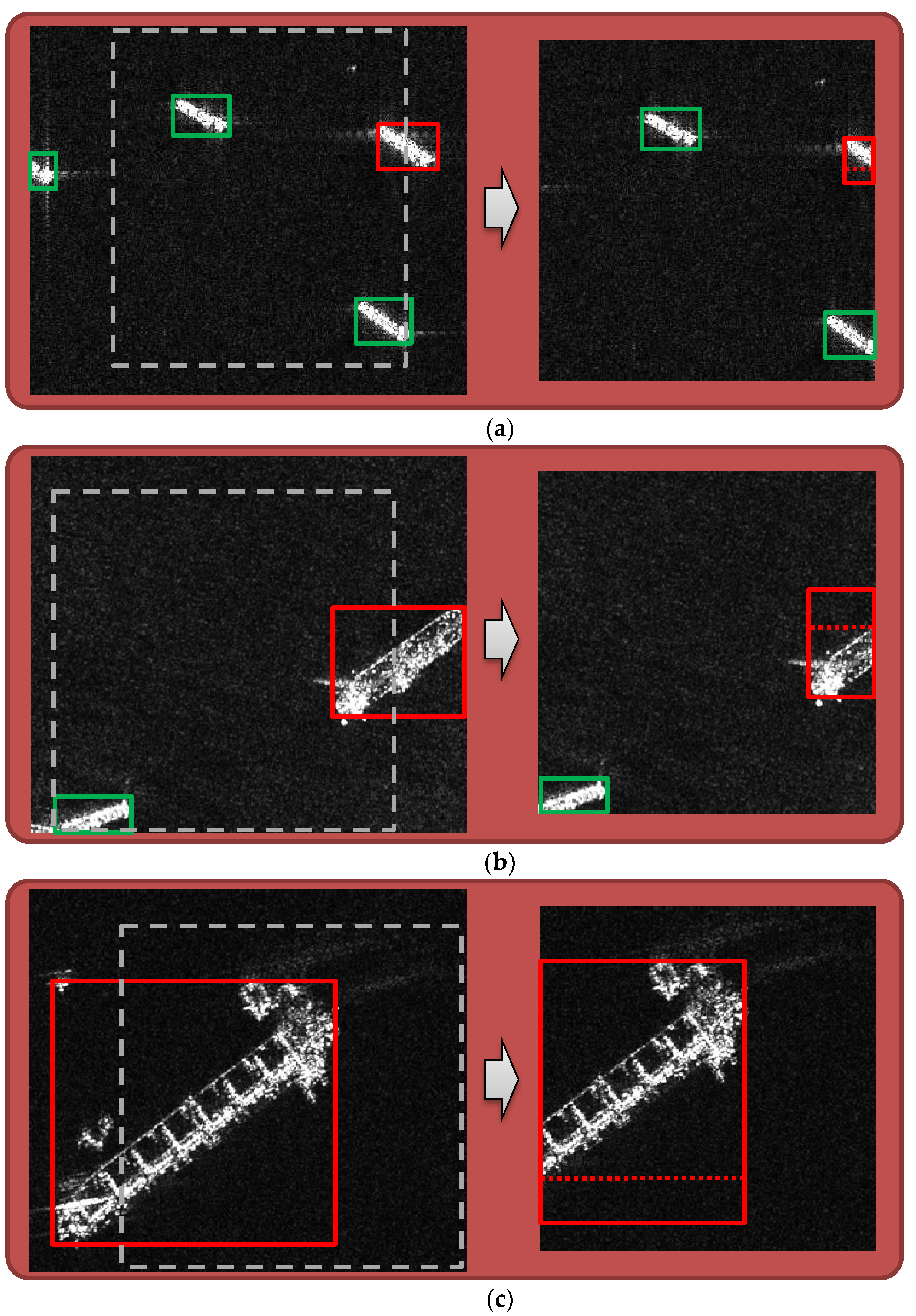
• A hidden source of training gradient noise introduced by the traditional random cropping data augmentation method is pointed out for the first time, which can lead to inaccurate target bounding box regression results and false alarm targets.
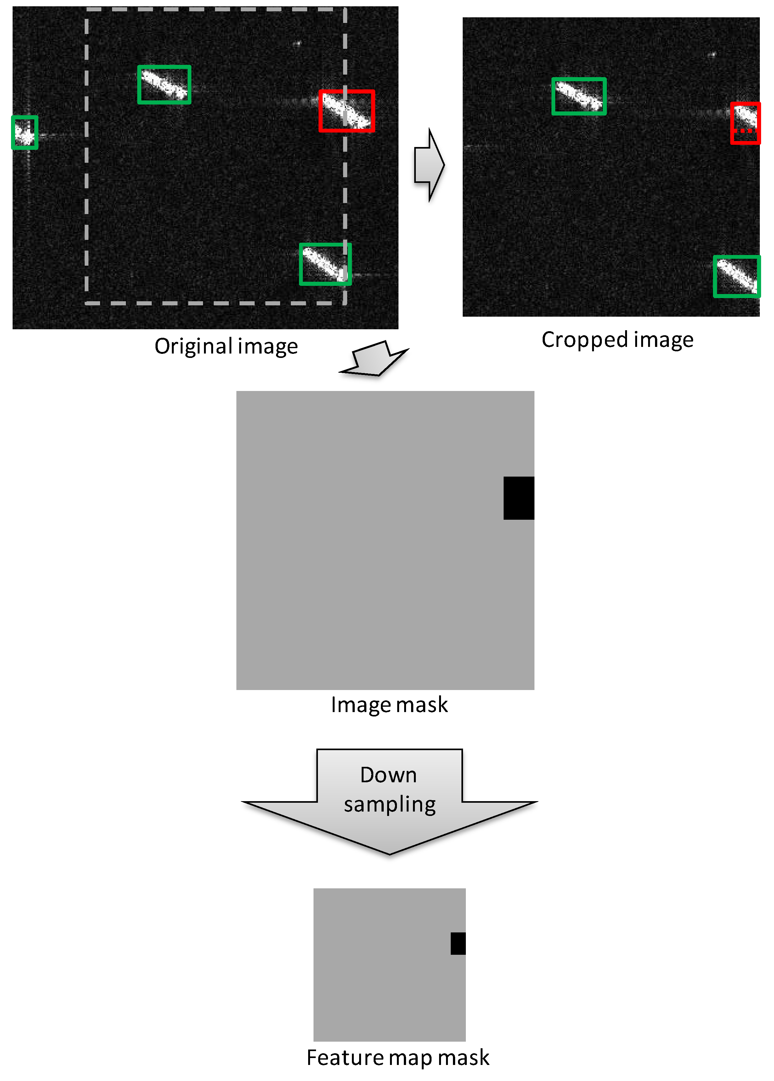
• A simple training method is proposed to suppress the gradient noise introduced by the traditional random cropping algorithm. This method uses a feature map mask to prevent pixels that generate gradient noise from participating in the calculation of training loss. The proposed method is proven to effectively improve the performance of the CNN-based SAR image ship detector, especially for high-precision bounding box regression tasks.

The remainder of the paper is organized as follows: Section 2 introduces the background of the problem, the basic network model used in this paper and the proposed training strategy for random cropping. Section 3 reports the experimental results on public dataset. Section 4 and Section 5 come to a discussion and conclusion.

2. Materials and Methods

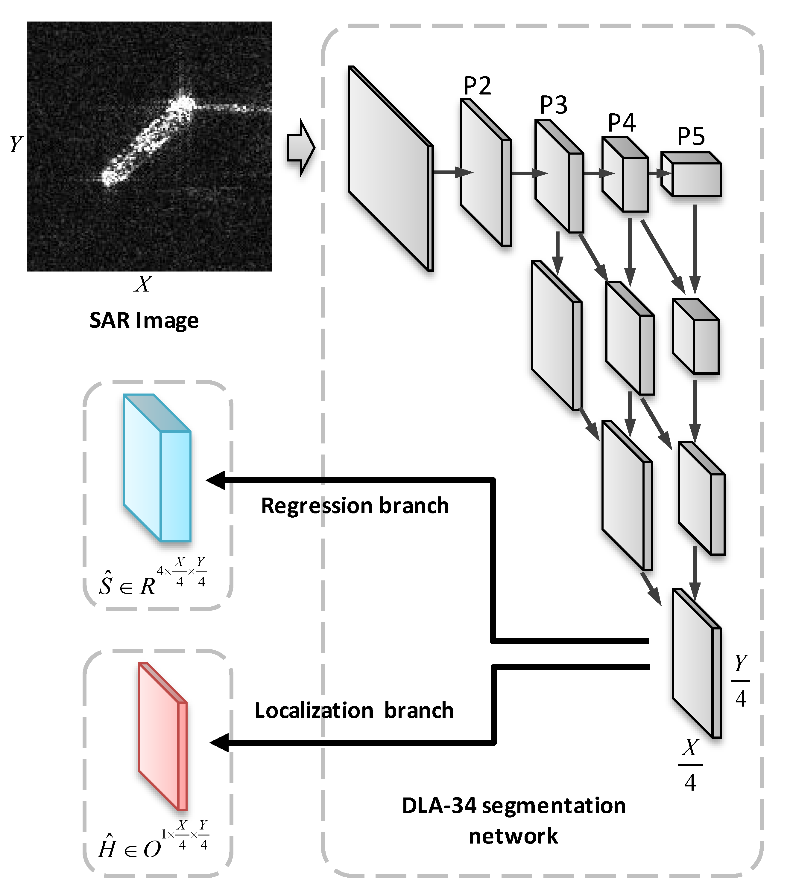
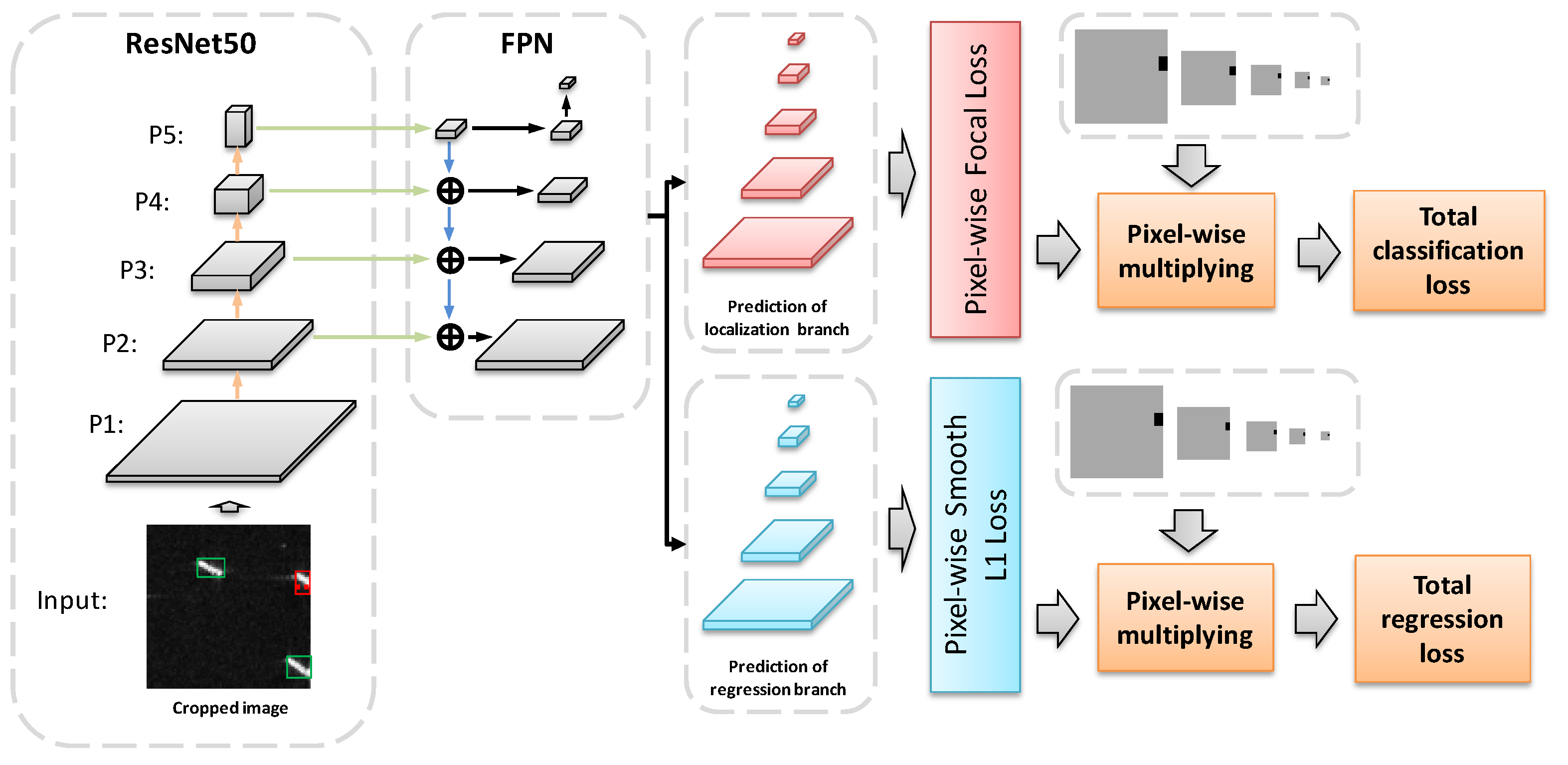
2.1. Basic Detection Model

This paper adopts a simplified CenterNet [12] model as the basic CNN model for testing the proposed training method, and we named our model as ShipDet. ShipDet uses DLA-34 [14] segmentation network as the basic structure. It uses the basic loss calculation method proposed in TTFNet [15] for training. The detailed structure of ShipDet is shown in Figure 1. Assuming the size of the input image is $X\times Y$, the DLA-34 segmentation network first performs feature extraction on the image and generates a feature map with a size of $\frac{X}{4}\times \frac{Y}{4}$. Then, the feature map is sent to two convolutional layers for target localization and bounding box regression, respectively.

The first convolution layer has a $1\times 1$ convolution kernel and 1 channel and it is followed by a sigmoid layer. Let $\widehat{H}$ be the output of this sigmoid layer where $\widehat{H}\in O^{1\times \frac{X}{4}\times \frac{Y}{4}}$, $O\in \left(0,1\right)$. $\widehat{H_{ij}}$ represents the probability that the pixel $(i,j)$ belongs to the center point of a target.

The size of the convolution kernel of the second convolution layer is $1\times 1$, and the number of channels is 4. Let $\widehat{S}$ be the output of the second convolution layer where $\widehat{S}\in R^{4\times \frac{X}{4}\times \frac{Y}{4}}$. If the pixel ($i,j$) is considered to be the center point of a target, ${\widehat{S}}_{ij}$ indicate the distance between the pixel ($i,j$) and the four sides of this bounding box.

In the training phase, the localization loss is calculated with modified focal loss [12] and the regression loss is calculated with L1 loss.

Given $m$-th annotated box, it is firstly linearly mapped to the feature map scale with stride of 4. Then, 2D Gaussian kernel $K_m\left(x,y\right)=exp(-\frac{{(x-x_0)}^2}{2{\sigma }_x^2}-\frac{{(y-y_0)}^2}{2{\sigma }_y^2})$ is adopted to produce $H_m\in R^{1\times \frac{X}{4}\times \frac{Y}{4}}$, where ${\sigma }_x=\frac{w}{12},{\sigma }_y=\frac{h}{12}$. $\left(x_0,y_0\right)$ represents the center point of the $m$-th box under the feature map scale and it is calculated as $\left(\mid \frac{x_m}{4}\mid ,\mid \frac{y_m}{4}\mid \right)$, where $\left(x_m,y_m\right)$ is the center point of the $m$-th box in the original image. $\left(w,h\right)$ are the width and height of the $m$-th box at the feature map scale. Finally, we generate the ground truth $H$ by applying element-wise maximum with $H_m$. Figure 2 shows a typical training image and its corresponding ground truth of localization branch.

Given the prediction $\widehat{H}$ and the ground truth $H$, the localization loss $L_{loc}$ is calculated as:

$$L_{loc}=\frac{1}{N}{\displaystyle \sum }_{x,y}\{\begin{array}{c}(1-{\widehat{H}}_{ij}{)}^{2}log({\widehat{H}}_{ij}),\hspace{1em}if{H}_{ij}=1\\ (1-H_{ij}{)}^4{\widehat{H}}_{ij}^{2}log(1-{\widehat{H}}_{ij}),\hspace{1em}else\end{array}$$

(1)

where $N$ is the number of targets in the training image.

Given $m$-th annotated box in the feature map scale, the ground truth of regression is given by $S\in R^{4\times \frac{X}{4}\times \frac{Y}{4}}$. Given pixel $(i,j)$ located inside the $m$-th annotated box in the feature map scale, $S_{ij}$ can be represented as a 4-dim vector ${(w_l,h_t,w_r,h_b)}_m$, which is defined as the distances from pixel $(i,j)$ to four sides of m-th box in the feature map scale with a normalization coefficient of 4. In other words, the predicted box $(x_1,y_1,x_2,y_2)$ in the original image scale can be represented as:

$$\begin{array}{c}{x}_1=4i-16w_l,y_1=4i-16h_t,\\ x_2=4i+16w_r,y_2=4i+16h_b,\end{array}$$

(2)

Let $A$ be the set of pixels where $H_{ij}>0$, then the regression loss is calculated as:

$$L_{reg}=\frac{1}{N_{reg}}{\displaystyle \sum }_{\left(i,j\right)\in A}L{1}_{loss}\left({\widehat{S}}_{ij},S_{ij}\right)\times W_{ij}$$

(3)

where $N_{reg}$ is the number of pixel where $H_{ij}>0$. $W_{ij}$ is a weight used to balance the loss of bounding boxes of different sizes, which will not affect our subsequent discussion. The calculation method of $W_{ij}$ can be found in [15]. The final total loss can be expressed as:

$$L=w_{loc}{L}_{loc}+w_{reg}{L}_{reg}$$

(4)

where $w_{loc}=1.0$ and $w_{reg}=5.0$ in our setting.

In the test phase, only the pixel corresponding to a peak point in the localization branch output feature map is considered as the center point of a predicted target bounding box, and the output of other pixels in the localization branch will be discarded.

Compared with the traditional anchor-based detection model such as RetinaNet [16] or Faster-RCNN [3], we found that this simplified anchor-free model has faster convergence speed (thanks to its faster inference speed) in the field of SAR ship detection, so we use it as the basic model to analyze our proposed method.

2.2. Training Gradient Noise Introduced by Random Cropping

The traditional random cropping data augmentation method used for target detection first randomly selects a target in the original image before cropping, and then it randomly crops an image slice under the premise that this target is included in the cropped image. After the cropped image slice is obtained, the cropping algorithm will automatically adjust the target bounding boxes in the image slice to ensure that the range of target bounding boxes in the image slice is limited to the range of the image slice.

The traditional random cropping algorithm does not introduce obvious errors in some detection tasks. Taking a vehicle detection training sample in the optical field shown in Figure 3 as an example, the two vehicle targets represented by the red box exceed the cropping range represented by the gray box, so the traditional random cropping algorithm automatically moves the edge of the red bounding box beyond the cropping range to the edge of the image slice. The traditional random cropping algorithm can ensure that the target bounding box at the edge of the image slice has sufficient accuracy for a horizontal target, such as a vehicle, which can be seen from Figure 3.

However, the orientation angle of many ship targets is not horizontal or vertical in the SAR image ship detection task, which makes the bounding boxes of the targets located at the edge of the slice in the randomly cropped image slice no longer accurate. Figure 4 shows three training samples containing ship targets of different scales. It can be seen from the red bounding box in the right column of Figure 4 that the target bounding boxes which cross the cropping boundary will be adjusted by the traditional random cropping algorithm. However, these target bounding boxes may still be inaccurate after the automatic adjustment. Part of the edge of the red bounding box should be adjusted to the red dotted line after random cropping. However, this operation cannot be done automatically by the random cropping algorithm, because the random cropping algorithm does not know the true boundary of each target.

If these training image slices generated by the traditional random cropping algorithm are used when training the SAR image ship detection model, those incorrect target borders will cause the model to make errors when calculating the training loss. These errors will introduce noise into the gradient in the back propagation process. Obviously, this gradient noise will hurt the learning process of the model, leading to the deterioration of model performance.

2.3. Training Method Proposed for SAR Ship Detection Models That Use Random Cropping as Data Augmentation

2.3.1. Feature Map Mask Used for the Guidance of Loss Calculation

Since traditional random cropping algorithm cannot automatically correct inaccurate target bounding boxes caused by random cropping, we can only try to eliminate the contribution of inaccurate target bounding boxes to training loss as much as possible during the model training process, thereby avoiding the introduction of noise into the training gradient. We propose to generate a feature map mask to guide the loss calculation, which is explained in Figure 5. When the random cropping algorithm generates an image slice, we generate a feature mask according to the target distribution in the image slice.

First, we generate a mask $M$ of the same size as the image slice and set the value of each pixel of the mask to 1.

Next, assuming that the $i$-th target bounding box in the original image crosses the cropping boundary, let $a_i$ be the area of the $i$-th target bounding box in the original image, and $b_i$ is the area of the $i$-th target bounding box automatically adjusted by the random cropping algorithm. If there is:

$$\frac{b_i}{a_i}<T_c$$

(5)

then, all the mask pixel values corresponding to the inside of the $i$-th target bounding box in the image slice will be set to 0. $T_c$ is used to control the tolerance of the model to the target bounding box error introduced by random cropping. Figure 6 shows an image containing four identical targets and an example of its cropping result. It can be found in Figure 6 that smaller $\frac{b_i}{a_i}$ means larger bounding box error for the same target. Figure 7 shows the corresponding image masks of the cropping result in Figure 6 under different $T_c$. In these masks, gray represents pixels with value 1, and black represents pixels with value 0. It can be seen from Figure 7 that a larger $T_c$ means less error introduced by random cropping in the model loss.

Finally, we downsample the mask $M$ to match the size of the feature map output by the model.

2.3.2. Loss Calculation with Feature Map Mask

After downsampling the mask $M$ to the size of the model output feature map, the mask $M$ will be added to the calculation of the model loss. Taking the simplified CenterNet model used in this paper as an example, the new localization loss $L_{loc}$ of the localization branch is:

$$L_{loc} = \frac{1}{N_1}{\displaystyle \sum }_{x,y}\{\begin{array}{c}(1 - {\widehat{H}}_{ij}{)}^{2}log({\widehat{H}}_{ij})M_{ij},\hspace{1em}if\hspace{0.17em}{H}_{ij} = 1\\ (1-H_{ij}{)}^4{\widehat{H}}_{ij}^{2}log(1-{\widehat{H}}_{ij})M_{ij},\hspace{0.17em}\hspace{1em}else\end{array}$$

(6)

where $N_1$ is equal to the total number of targets in the image slice minus the number of targets with $\frac{b_i}{a_i}<T_c$.

The new regression loss is calculated as:

$$L_{reg}=\frac{1}{N_2}{\displaystyle \sum }_{(i,j)\in A}L{1}_{loss}({\widehat{S}}_{ij},S_{ij})\times W_{ij}\times M_{ij}$$

(7)

where $N_2$ is the number of pixel where $H_{ij}>0$ and $M_{ij}=1$.

It can be seen from the new loss functions that if the $i$-th target in the image slice satisfies $\frac{b_i}{a_i}<T_c$, then the loss contribution of the pixel inside the $i$-th target bounding box in the image slice will be equal to 0, which avoids introducing errors into the total loss.

It should be noted that if the orientation angle of a ship target is vertical or horizontal and its bounding box crosses the cropping boundary, the bounding box of this target still has high accuracy after adjusted by the random clipping algorithm. Although its contribution to the training loss will still be suppressed by the mask when this target box satisfies $\frac{b_i}{a_i}<T_c$, its impact on the model is not obvious, so we do not do special treatment for this situation.

2.4. Implementation Details

2.4.1. Data Preprocessing and Post-Processing

During the training phase, each training image will be randomly cropped into $C\times C$ slices and randomly flipped horizontally. During the test phase, According to [15], a maxpooling layer with a kernel size of $3\times 3$ is used to extract the peak points in the output feature map of the localization branch, and all peak points with a peak value greater than $T_{conf}$ will be considered as positive targets. $T_{conf}$ is set to 0.05 in our experiments. The output results of the regression branch corresponding to the peak points will be used to decode the bounding box position of the targets, according to Equation (2).

2.4.2. Optimizer Setting

All of the models are trained with Stochastic Gradient Descent (SGD) algorithm over an Intel i9-9700k processor and an NVidia GTX1080Ti GPU. The mini-batch size is 4 in each iteration. A small batch size is selected here to increase the total number of iterations as much as possible without increasing too much training time too much, which is beneficial to increase the number of randomly crop times of each image and shown a better compromise between training time and model accuracy in our experiments. All models are trained for 150 epochs. The cosine annealing learning rate scheduling strategy is adopted with an initial learning rate of 0.001.

3. Results

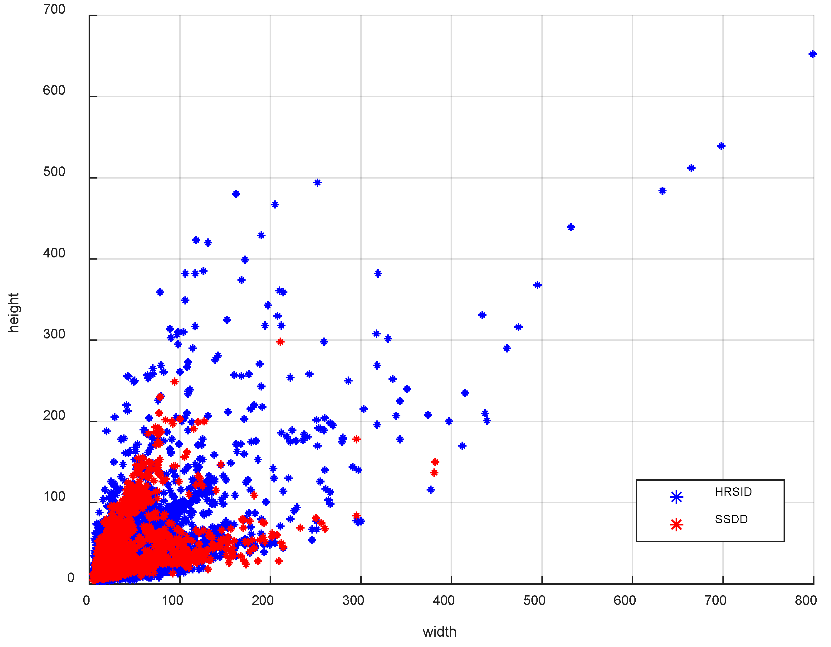
3.1. Experimental Data

In this paper, HRSID [17] dataset is used to test the proposed method. HRSID is a large SAR ship detection dataset published recently which contains multi-scale ships labeled with bounding box in various environments, including different scenes, sensor types and polarization modes. It has more training samples and test samples than classic SAR ship detection dataset SSDD [18], which can help researchers evaluate their methods more accurately. Some important parameters of HRSID are shown in

Table 1. The main parameters of HRSID.

Parameter	Value
Size of images (Pixel)	$800\times 800$
Number of training images	3642
Number of testing images	1962
Resolution (m)	0.5∼3
Polarization	HH, VV, HV
Satellite	Sentinel-1B, TerraSAR-X, TanDEM
Range of incident angle (◦)	20∼60
Background type	Inshore, Offshore
Total number of ships	16,906

. Figure 8 shows the distribution of the length and width of the target bounding boxes in the HRSID and SSDD. It can be seen from the distribution that HRSID has a larger target scale variation range, which brings a greater challenge to the robustness of the detector. More detailed information about HRSID can be found in [17].

3.2. Evaluation Criteria

In order to quantitatively evaluate the effectiveness of the proposed method, standard PASCAL VOC evaluation indicators [19] are used to compare the performance of different configurations.

For typical CNN-based detection models, a specific Intersection-over-Union (IoU) threshold will be used to filter out detection results with low confidence. The precision rate $P_r$ of the model will increase as the threshold increases, but the recall rate $R_r$ of the model will decrease. Recall rate $R_r$ is the ratio of true positive targets (TP) in all ground truths, which is defined as:

$$R_r=\frac{TP}{TP+FN}$$

(8)

where $FN$ means false negative targets. Precision rate $P_r$ is the ratio of TPs in all detected targets. The definition is as follows:

$$P_r=\frac{TP}{TP+FP}$$

(9)

where $FP$ means false positive targets. AP is the standard metric for target detection algorithms, which comprehensively considers the $P_r$ and $R_r$ of the model at different confidence levels and can be expressed as:

$$\mathrm{AP}={{\displaystyle \int }}_0^1{P}_r\left(R_r\right){\mathrm{d}R}_r$$

(10)

The $AP$ of an ideal detector will be equal to 1. Three kinds of AP indicators including mAP, AP50, and AP75 are used in this paper. The meanings of mAP, AP50, and AP75 are shown in

Table 2. Evaluation Metrics used in this paper.

Metrics	Metrics Meaning
mAP	AP average from IoU = 0.50: 0.05: 0.95
AP50	AP at IoU = 0.50
AP75	AP at IoU = 0.75

.

3.3. Evaluation Results of the Proposed Method

In the random cropping process, the size $C$ of the image slice is often fixed to an integer multiple of the maximum downsampling multiple of the model in order to ensure that the feature map is always divisible when performing downsampling operation. Models with $T_c=0.7$ and $C$ from 704 to 416 were trained and tested in order to analyze the robustness of the proposed method under different random crop sizes. The test results of different configurations are summarized in

Table 3. Test results of different configurations. Bold values refer to the best one.

Crop Size	Method	mAP (%)	AP50 (%)	AP75 (%)
800	No random crop	66.43	88.61	76.86
704	Traditional method	67.36	90.16	78.13
	Proposed method	68.21	91.61	79.70
608	Traditional method	67.18	91.04	77.60
	Proposed method	68.17	91.99	79.38
512	Traditional method	67.40	90.94	78.09
	Proposed method	68.50	91.51	79.29
416	Traditional method	67.30	91.31	77.49
	Proposed method	68.23	91.47	78.85

. Figure 9, Figure 10 and Figure 11 show the comparison of model performance on test set under different $C$. $C=800$ means that the model is trained without random cropping.

In order to analyze the impact of different $T_c$ on model performance, models with different $T_c$ under $C=512$ were trained and compared.

Table 4. Test results of different $T_c$.

$T_c$	mAP (%)	AP50 (%)	AP75 (%)
0	67.4	90.94	78.09
0.1	67.65	91.43	77.63
0.2	67.66	91.25	78.03
0.3	67.51	91.19	77.88
0.4	67.79	91.36	78.42
0.5	67.88	91.36	79.04
0.6	68.04	91.61	78.77
0.7	68.50	91.51	79.29
0.8	67.75	91.14	78.53
0.9	67.50	91.04	78.07

gives the summary of the test results under different $T_c$. The visualization results under different metrics are given in Figure 12, Figure 13 and Figure 14. In addition to the detection performance of the models under different $T_c$, we also counted the number of target bounding boxes participating in the loss calculation and the number of target bounding boxes not participating in the loss calculation (suppressed by the mask) in an epoch under different $T_c$. The statistical results are shown in Figure 15.

Figure 16 and Figure 17 show a part of detection results of the models after training with the traditional random cropping algorithm and the proposed method ($T_c=0.7$) when $C=512$. Figure 18 show the enlarged comparison images of some typical targets in Figure 16 and Figure 17 for a clearer view.

In addition to the anchor-free model proposed in the paper, we have also verified the proposed method on typical anchor-based model RetinaNet. Our modified RetinaNet uses feature maps from P2, P3, P4, P5, and P6 for prediction instead of the original P3–P7. The introduction of P2 feature map greatly improved the detection accuracy of the model on HRSID because the feature map from P2 has a higher resolution, which is beneficial to the detection of a large number of small ships in HRSID. Except for the model itself, other implementation details remain the same as in Section 2.4.2. Like ShipDet, the predicted value of each pixel in the output feature map of different scales of RetinaNet will be multiplied by the feature map mask of the corresponding scale after calculating the loss with ground truth, which avoids the pixels inside the target bounding box with large errors to participate in the final loss summation. The detailed loss calculation process of RetinaNet with the proposed method is shown in Figure 19. The experimental results are shown in

Table 5. Experimental results on anchor-based model RetinaNet (ResNet50).

Crop Size	Method	mAP (%)	AP50 (%)	AP75 (%)
800	No random crop	63.61	88.59	74.64
512	Traditional method	66.22	91.20	76.68
	Proposed method ($T_c=0.7$)	67.61	91.89	78.25

.

4. Discussion

4.1. Analysis of the Proposed Method under Different Metrics

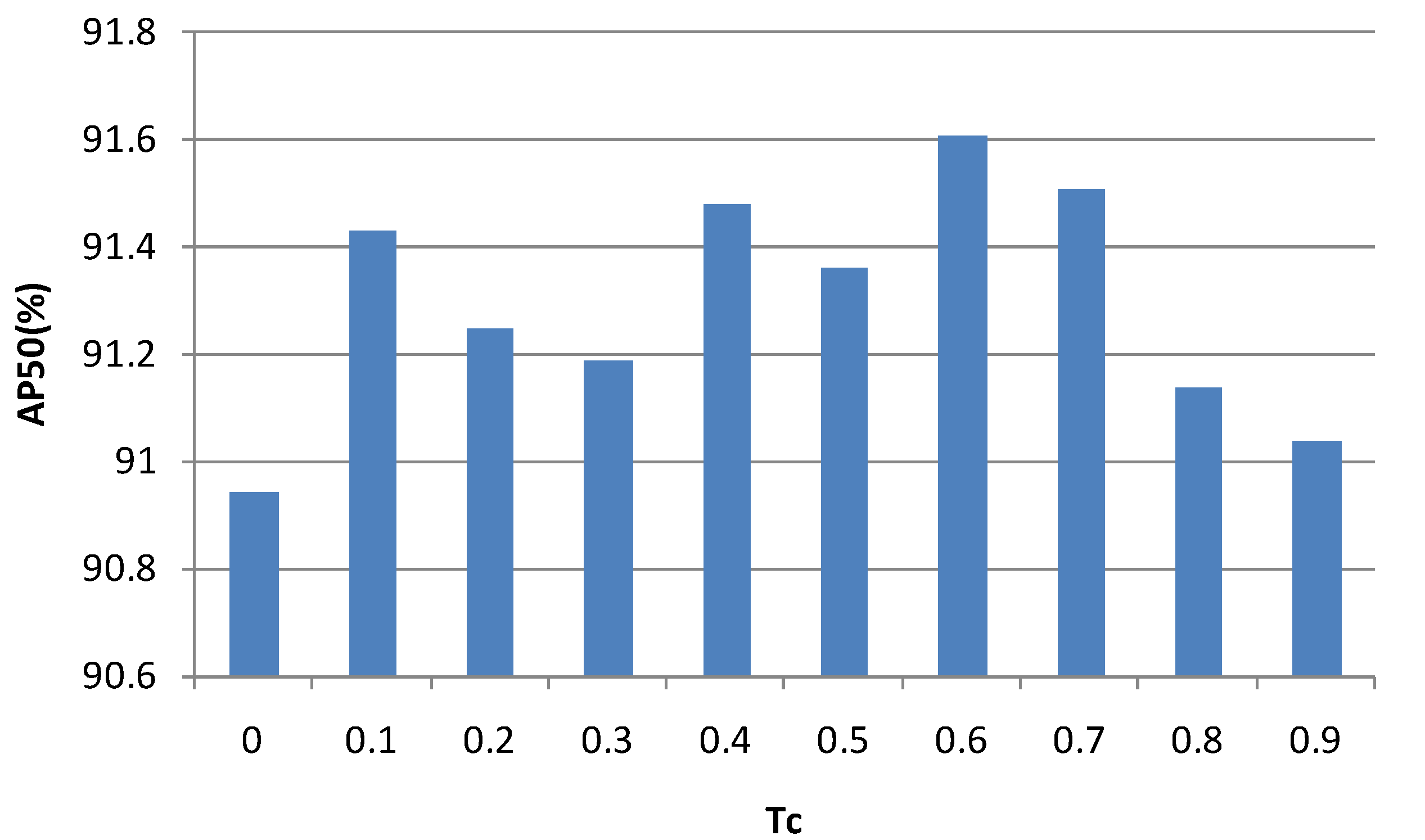
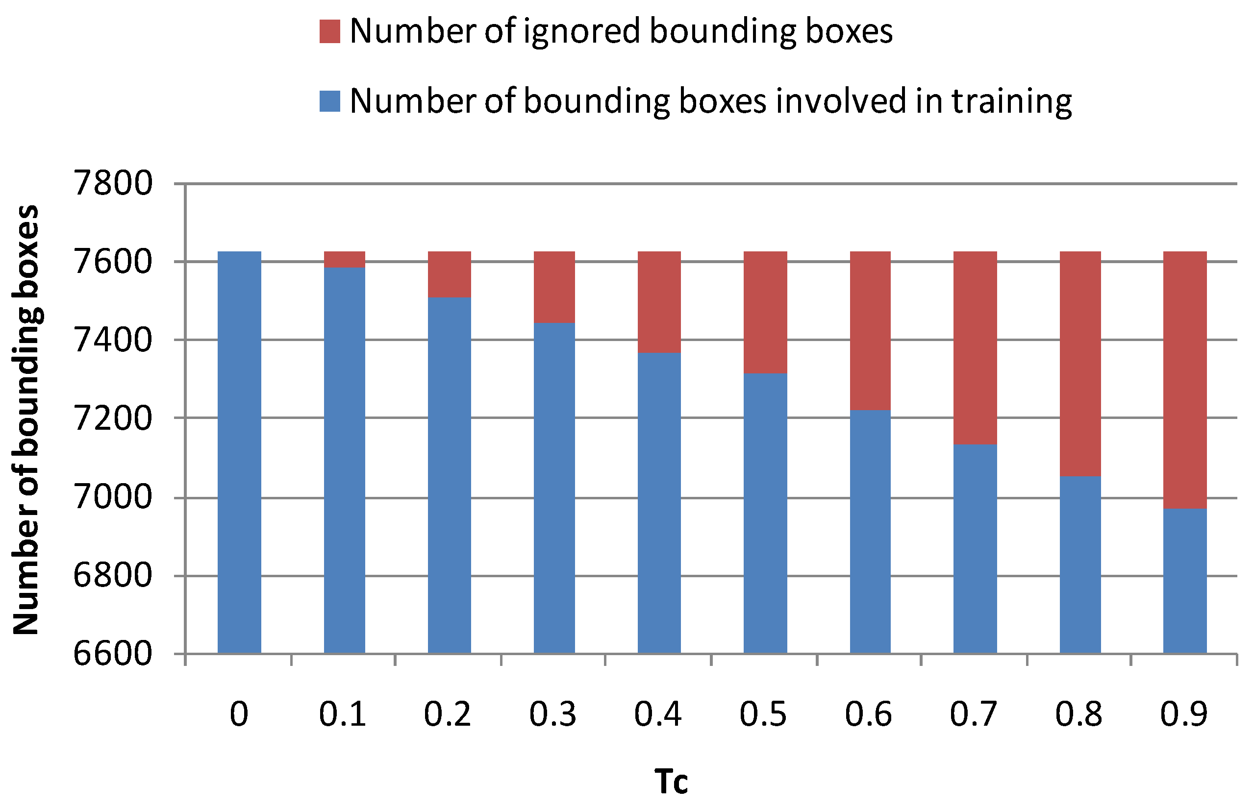
At least three conclusions can be drawn from the comparison results of Figure 9, Figure 10 and Figure 11. First, the use of random cropping can effectively improve the detection performance of the model under different indicators. Second, the proposed method can significantly improve the detection performance of the model under different crop sizes, which not only proves the effectiveness of the proposed method, but also shows that it is inappropriate to ignore the gradient noise introduced by traditional random cropping algorithm. Third, compared with the results of AP50, eliminating the gradient error introduced by the random cropping algorithm can achieve a more obvious and stable performance improvement on AP75, which illustrates that the high-precision bounding box regression task is more sensitive to the gradient error introduced by the random cropping algorithm. In addition, Table 5 also proves that the proposed method is not only applicable to the anchor-free CNN model, but can also bring significant performance improvements in the typical anchor-based CNN model.

4.2. The Influence of Different $T_c$ on the Performance of the Proposed Method

From the change trend of different metrics in Figure 12, Figure 13 and Figure 14, it can be seen that there is a peak of model performance around $T_c=0.7$. In theory, a larger $T_c$ means that the random cropping algorithm introduces less gradient noise. When $T_c$ is large, even if the targets at the edge of the image have a small bounding box error, they will still not be able to participate in the training of the model, which is explained in Figure 6 and Figure 7 and can be proved by Figure 15. However, the experimental results show that the performance of the model declines rapidly when $T_c$ is close to 1, which shows that the target bounding boxes with low error at the edge of the image are still benefit to the model’s learning and it is not appropriate to simply remove the loss contribution of all targets located at the boundary of the image.

4.3. Analysis of the Ship Detection Results

Figure 16 and Figure 17 show examples of detection results for targets of different scales using the model trained with traditional random cropping method and the proposed method. It can be seen from the detection results that the bounding box regression accuracy of the model trained by the proposed method is better than that of the model trained by the traditional random cropping method on many targets at the edge of the image. The detection performance of these two methods in the middle of the image has little difference. This may be because the gradient noise introduced by the traditional random cropping method is mainly from the edges of the training image. In addition, it can be found that the model trained with the traditional random cropping method is also prone to produce many strange false alarm targets at the edge of the image. This shows that the gradient noise introduced by the traditional random cropping method not only affects the model’s box regression ability, but also hurts the ability to determine whether the target exists.

4.4. The Significance of theProposed Method for SAR Image Ship Detection Task

Effective data augmentation methods are essential for the CNN-based model when training data is very limited. Considering that the training data of the SAR image ship detection task is often more limited compared with the optical image detection task, our method has sufficient value for the SAR image ship detection task.

4.5. Applicability of the Proposed Method in Other Fields

The method proposed in this paper is dedicated to suppress the gradient noise when training the CNN-based SAR image ship detector using the traditional random cropping method. However, it is foreseeable that this method is also applicable to other detection scenarios, in which most targets have extremely large aspect ratios and different orientation angles. One of the most intuitive examples is ship detection based on optical remote sensing images.

5. Conclusions

In this paper, the problem of gradient noise introduced by traditional random cropping algorithm when training CNN-based SAR image ship detection model is pointed out for the first time, which has been proven to cause the deterioration of detection performance, especially for high-precision bounding box regression tasks. Then, a simple and effective method is proposed for the suppression of the gradient noise. The experimental results show that the proposed method can effectively eliminate the gradient noise introduced by random cropping, thereby improving the model’s detection performance without affecting the detection efficiency of the model.

References

1. Redmon, J.; Divvala, S.; Girshick, R.; Farhadi, A. You only look once: Unified, real-time object detection. In Proceedings of the IEEE Conference on Computer Vision and Pattern Recognition, Las Vegas, NV, USA, 27–30 June 2016; pp. 779–788. [Google Scholar]
2. Liu, W.; Anguelov, D.; Erhan, D.; Szegedy, C.; Reed, S.; Fu, C.-Y.; Berg, A.C. Ssd: Single shot multi box detector. In European Conference On computer Vision; Springer: Cham, Switzerland, 2016; pp. 21–37. [Google Scholar]
3. Ren, S.; He, K.; Girshick, R.; Sun, J. Faster r-cnn: Towards real-time object detection with region proposal networks. In Proceedings of the Advances in Neural information Processing Systems; MIT Press: Cambridge, MA, USA, 2015; pp. 91–99. [Google Scholar]
4. An, Q.; Pan, Z.; Liu, L.; You, H. Drbox-v2: An improved detector with rotatable boxes for target detection in sar images. IEEE Trans. Geosci. Remote Sens. 2019, 57, 8333–8349. [Google Scholar] [CrossRef]
5. Wang, Y.; Wang, C.; Zhang, H.; Dong, Y.; Wei, S. Automatic ship detection based on retinanet using multi-resolution gaofen-3 imagery. Remote Sens. 2019, 11, 531. [Google Scholar] [CrossRef] [Green Version]
6. Wei, S.; Su, H.; Ming, J.; Wang, C.; Yan, M.; Kumar, D.; Shi, J.; Zhang, X. Precise and robust ship detection for high-resolution sar imagery based on hr-sdnet. Remote Sens. 2020, 12, 167. [Google Scholar] [CrossRef] [Green Version]
7. Zhang, T.; Zhang, X.; Shi, J.; Wei, S. Depth wise separable convolution neural network for high-speed sar ship detection. Remote Sens. 2019, 11, 2483. [Google Scholar] [CrossRef] [Green Version]
8. Cui, Z.; Li, Q.; Cao, Z.; Liu, N. Dense attention pyramid networks for multi-scale ship detection in sar images. In IEEE Transactions on Geoscience and Remote Sensing; IEEE: Piscataway, NJ, USA, 2019; Volume 57, pp. 8983–8997. [Google Scholar]
9. Wu, X.; Sahoo, D.; Hoi, S.C. Recent advances in deep learning for object detection. Neurocomputing 2020. [Google Scholar] [CrossRef] [Green Version]
10. Bochkovskiy, A.; Wang, C.-Y.; Liao, H.-Y.M. Yolov4: Optimal speed and accuracy of object detection. arXiv 2020, arXiv:2004.10934. Available online: https://arxiv.org/abs/2004.10934 (accessed on 29 April 2020).
11. Yun, S.; Han, D.; Oh, S.J.; Chun, S.; Choe, J.; Yoo, Y. Cutmix: Regularization strategy to train strong classifiers with localizable features. In Proceedings of the IEEE International Conference on Computer Vision, Seoul, Korea, 27 October–3 November 2019; pp. 6023–6032. [Google Scholar]
12. Zhou, X.; Wang, D.; Krähenbühl, P. Objects as points. arXiv 2019, arXiv:1904.07850. Available online: https://arxiv.org/abs/1904.07850 (accessed on 16 April 2020).
13. Chen, C.; He, C.; Hu, C.; Pei, H.; Jiao, L. A deep neural network based on an attention mechanism for sar ship detection in multi scale and complex scenarios. IEEE Access 2019, 7, 104848–104863. [Google Scholar] [CrossRef]
14. Yu, F.; Wang, D.; Shelhamer, E.; Darrell, T. Deep layer aggregation. In Proceedings of the IEEE Conference on Computer Vision and Pattern Recognition, Salt Lake City, UT, USA, 18–23 June 2018; pp. 2403–2412. [Google Scholar]
15. Liu, Z.; Zheng, T.; Xu, G.; Yang, Z.; Liu, H.; Cai, D. Training-Time-Friendly Network for Real-Time Object Detection; AAAI: Menlo Park, CA, USA, 2020; pp. 11685–11692. [Google Scholar]
16. Lin, T.-Y.; Goyal, P.; Girshick, R.; He, K.; Dollar, P. Focal loss for dense object detection. In Proceedings of the IEEE International Conference on Computer Vision, Venice, Italy, 22–29 October 2017; pp. 2980–2988. [Google Scholar]
17. Wei, S.; Zeng, X.; Qu, Q.; Wang, M.; Su, H.; Shi, J. Hrsid: A high-resolution sar images dataset for ship detection and instan cesegmentation. IEEE Access 2020, 8, 120234–120254. [Google Scholar] [CrossRef]
18. Li, J.; Qu, C.; Shao, J. Ship detection in sar images based on an improved faster r-cnn. In Proceedings of the 2017 SAR in Big Data Era: Models, Methods and Applications (BIGSARDATA), Beijing, China, 13–14 November 2017; IEEE: Piscataway, NJ, USA, 2017; pp. 1–6. [Google Scholar]
19. Everingham, M.; van Gool, L.; Williams, C.K.; Winn, J.; Zisserman, A. The Pascal Visual Object Classes Challenge 2007 (voc2007) Results. 2007. Available online: http://host.robots.ox.ac.uk/pascal/VOC/voc2007/ (accessed on 29 April 2020).
Figure 1. The architecture of ShipDet.
Remotesensing 13 00034 g001
Figure 2. Training image and its corresponding ground truth of localization branch. (a) A typical training image. (b) The corresponding ground truth of localization branch in original image scale.
Remotesensing 13 00034 g002
Figure 3. A training sample of vehicle detection and an example of its random cropping result.
Remotesensing 13 00034 g003
Figure 4. Three training samples of synthetic aperture radar (SAR) ship detection (left column) and examples of their random cropping results (right column). (a) Sample of small size targets. (b) Sample of medium size targets. (c) Sample of large size target.
Remotesensing 13 00034 g004
Figure 5. Image slice and its corresponding feature map mask.
Remotesensing 13 00034 g005
Figure 6. Bounding box error of different targets.
Remotesensing 13 00034 g006
Figure 7. Masks under different T c .
Remotesensing 13 00034 g007
Figure 8. Distribution of bounding box length and width of HRSID and SSDD.
Remotesensing 13 00034 g008
Figure 9. mAP of different models under different random crop sizes.
Remotesensing 13 00034 g009
Figure 10. AP50 of different models under different random crop sizes.
Remotesensing 13 00034 g010
Figure 11. AP75 of different models under different random crop sizes.
Remotesensing 13 00034 g011
Figure 12. mAP of models under different T c .
Remotesensing 13 00034 g012
Figure 13. AP50 of models under different T c .
Remotesensing 13 00034 g013
Figure 14. AP75 of models under different T c .
Remotesensing 13 00034 g014
Figure 15. The number of bounding boxes involved in loss calculation and the number of bounding boxes of targets not involved in loss calculation (suppressed by the mask) in a training epoch.
Remotesensing 13 00034 g015
Figure 16. Comparison of detection results between traditional random cropping algorithm (left column in each panel) and the proposed method (right column in each panel) on small targets. The green boxes represent the true bounding boxes of the targets that were successfully detected. The blue boxes indicate the true bounding boxes of the targets that were not successfully detected. The red boxes represent the model prediction results, and the number on the red box represents the model’s confidence in this prediction result. (a) Example 1; (b) Example 2; (c) Example 3; (d) Example 4.
Remotesensing 13 00034 g016aRemotesensing 13 00034 g016b
Figure 17. Comparison of detection results between traditional random cropping algorithm (left column in each panel) and the proposed method (right column in each panel) on medium and large targets. The green boxes represent the true bounding boxes of the targets that were successfully detected. The blue boxes indicate the true bounding boxes of the targets that were not successfully detected. The red boxes represent the model prediction results, and the number on the red box represents the model’s confidence in this prediction result. (a) Example 5; (b) Example 6; (c) Example 7; (d) Example 8.
Remotesensing 13 00034 g017aRemotesensing 13 00034 g017b
Figure 18. Enlarged comparison images of some typical targets in Figure 16 and Figure 17 between traditional random cropping algorithm (left column in each panel) and the proposed method (right column in each panel). The green boxes represent the true bounding boxes of the targets that were successfully detected. The blue boxes indicate the true bounding boxes of the targets that were not successfully detected. The red boxes represent the model prediction results, and the number on the red box represents the model’s confidence in this prediction result. (a) Example 9; (b) Example 10; (c) Example 11; (d) Example 12.
Remotesensing 13 00034 g018aRemotesensing 13 00034 g018b
Figure 19. Loss calculation process of RetinaNet with the proposed method.
Remotesensing 13 00034 g019