A Practical Cross-View Image Matching Method between UAV and Satellite for UAV-Based Geo-Localization


1
School of Resources and Environment, Center for Information Geoscience, University of Electronic Science and Technology of China, Chengdu 611731, China
2
The Yangtze Delta Region Institute (Huzhou), University of Electronic Science and Technology of China, Huzhou 313001, China
3
College of Meteorology and Oceanography, National University of Defense Technology, Nanjing 211101, China
*
Author to whom correspondence should be addressed.
Remote Sens. 2021, 13(1), 47; https://0-doi-org.brum.beds.ac.uk/10.3390/rs13010047
Submission received: 8 December 2020
/
Revised: 21 December 2020
/
Accepted: 22 December 2020
/
Published: 24 December 2020
(This article belongs to the Special Issue Computer Vision and Deep Learning for Remote Sensing Applications)
Abstract
:Cross-view image matching has attracted extensive attention due to its huge potential applications, such as localization and navigation. Unmanned aerial vehicle (UAV) technology has been developed rapidly in recent years, and people have more opportunities to obtain and use UAV-view images than ever before. However, the algorithms of cross-view image matching between the UAV view (oblique view) and the satellite view (vertical view) are still in their beginning stage, and the matching accuracy is expected to be further improved when applied in real situations. Within this context, in this study, we proposed a cross-view matching method based on location classification (hereinafter referred to LCM), in which the similarity between UAV and satellite views is considered, and we implemented the method with the newest UAV-based geo-localization dataset (University-1652). LCM is able to solve the imbalance of the input sample number between the satellite images and the UAV images. In the training stage, LCM can simplify the retrieval problem into a classification problem and consider the influence of the feature vector size on the matching accuracy. Compared with one study, LCM shows higher accuracies, and Recall@K (K ∈ {1, 5, 10}) and the average precision (AP) were improved by 5–10%. The expansion of satellite-view images and multiple queries proposed by the LCM are capable of improving the matching accuracy during the experiment. In addition, the influences of different feature sizes on the LCM’s accuracy are determined, and we found that 512 is the optimal feature size. Finally, the LCM model trained based on synthetic UAV-view images was evaluated in real-world situations, and the evaluation result shows that it still has satisfactory matching accuracy. The LCM can realize the bidirectional matching between the UAV-view image and the satellite-view image and can contribute to two applications: (i) UAV-view image localization (i.e., predicting the geographic location of UAV-view images based on satellite-view images with geo-tags) and (ii) UAV navigation (i.e., driving the UAV to the region of interest in the satellite-view image based on the flight record).

1. Introduction
Remote sensing technology has been developed rapidly in the past few decades, and remote sensing platforms have gradually become diversified, such as ground, aerial, and satellite platforms. Satellites, airplanes, and unmanned aerial vehicles (UAVs) have been the main carriers in the acquisition of remote sensing images. In particular, the UAV has the advantages of strong maneuverability, convenient operation, being hardly influenced by cloud, strong data acquisition abilities [1,2,3], etc., which make it widely applied in various fields [4,5,6,7,8,9,10,11,12]. How to efficiently locate the UAV images without geo-tags and navigate the UAV when the positioning system (e.g., GPS) is not available still face great challenges that are expected to be solved. Image-based geo-localization is an emerging technology in cross-view information integration and provides a new idea for UAV image localization and navigation. It is able to locate images without geo-tags based on images with geo-tags, so as to better serve UAV image localization and navigation. The key to solving this problem is the cross-view image matching between the images without geo-tags and the images with geo-tags.
Early studies of cross-view image matching are based on the ground view [13,14,15,16]. However, the ground-view images with geo-tags are usually limited to small spatial and temporal scales and are difficult to obtain. In contrast, satellite-view images have the advantages of wide spatiotemporal coverages and having geo-tags. Some traditional satellite-view image processing methods (e.g., image classification, object detection, and semantic segmentation) simply use the surface feature information captured by satellite images [17,18,19,20,21,22,23,24,25,26], and the geo-tags of the satellite-view image are usually neglected. To make full use of the geo-tags of the satellite-view images to locate images from other views, scientific communities began to pay attention to cross-view image matching between the satellite view and other views. A large series of image datasets for cross-view image matching, which usually come from the ground view and the satellite view, has been released. Lin et al. [27] used public image data sources to construct 78,000 image pairs between aerial images and ground-view images. Inspired by this idea, Tian et al. [28] collected ground-view (street-view) images and aerial-view images of buildings in different cities (including Pittsburg, Orlando, and Manhattan) and produced image pairs. Besides the above two datasets, CVUSA [29] and CVACT [30] are the other two datasets related to cross-view image matching. At the same location in CVUSA and CVACT datasets, there is an image pair, which contains a panoramic ground-view image and a satellite-view image.
Based on these datasets, a series of cross-view image matching methods were developed [29,30,31,32,33,34,35,36,37]. Bansal et al. [31] used the structure of self-similarity of patterns on facades to match ground-view images to an aerial gallery, which demonstrated the feasibility of matching the ground-view image with the aerial-view image. Lin et al. [32] used the mean of aerial image features or ground attribute image features as labels. Then, they used support vector machines (SVMs) to classify ground-view images to realize the cross-view image matching. With the continuous development of deep learning, the convolutional neural network (CNN) has shown good performance in image feature expression [36,38,39,40,41]. Since then, CNN has been widely used for cross-view image matching.
The methods of using CNN can be divided into two types. The first method is to align the image features of one view with the features of another view. Lin et al. [32] used CNN to search for the matching factor between the aerial-view and ground-view images and found the matching accuracy was significantly improved, which laid a good foundation for later scientists to use deep learning technology to realize cross-view image matching. After extracting the building through the method of target detection, Tian et al. [28] used the building as a bridge between the ground-view and the aerial-view images to perform cross-view image matching and achieve the goal of geo-localization in the urban environment. Based on the CVUSA dataset, Zhai et al. [29] proposed a strategy for extracting the semantic features of the satellite view. They first extracted the features of the satellite-view image through CNN and then mapped these extracted features to the ground view to obtain ground-like view features. Finally, the ground-like view features were compared with the semantic features extracted directly from the ground-view image, and the difference was minimized through end-to-end training. The ground-like view features extracted by the model were matched with the ground-view features in the test set to complete the cross-view image matching and realize the geo-localization. Since then, CVUSA has been widely used in cross-view image matching studies, and a series of methods have been proposed. Hu et al. [42] used a two-branch CNN to extract the local features of the ground-view image and the satellite-view image, and then used the Netvlad layer to aggregate the extracted local features to obtain a global description vector [43,44]. Through end-to-end training, the global description vector distance of positive samples between two views is minimized, and the negative sample distance is maximized. Finally, based on the distance of the global description vector of the two views, the cross-view image matching at the same location is realized. Shi et al. [45] also used a two-branch CNN to extract image features from two views. Instead of directly optimizing the distance between positive and negative samples, they recombined ground-view features through feature transport to obtain satellite-like view features. They optimized the distance between the satellite-view feature and the satellite-like view feature. Based on the CVACT dataset, Liu and Li [30] added the orientation information in the panoramic ground-view image to the deep learning network model, which shows an outstanding performance in the matching between the panoramic ground-view image and the satellite-view image. This method provides a novel perspective for the cross-view image matching.
The second method is to map the features of different views to the same space according to the idea of classification. The dataset used in the first method usually has only one image pair at a target location (only one image of each view). Therefore, it is infeasible to use images from different views of a target location as a class to learn the image features of the same location. The images from different views of a target location were used as a class in the second method. Workman and Jacobs [36] found that the classification model trained on the place dataset performed well in the feature recognition of other places. Zheng et al. [46] used two-branch CNN and category labels to match the UAV-view, satellite-view, and ground-view images.
The existing cross-view image matching methods are mostly aimed at the aerial view (including satellite view) and the ground view and use a dataset that only has a single image pair at the target location. However, these methods do not consider the similarity between the satellite-view image and the UAV-view image, which makes them difficult to be used for cross-view image matching between the satellite view and the UAV view. To overcome the shortcomings of existing methods in cross-view image matching between the satellite view and the UAV view, we proposed a cross-view image matching method based on location classification (LCM). In this paper, the impact of expanding a single satellite image, the length of image features, and multiple queries on matching accuracy are also explored.
2. Datasets
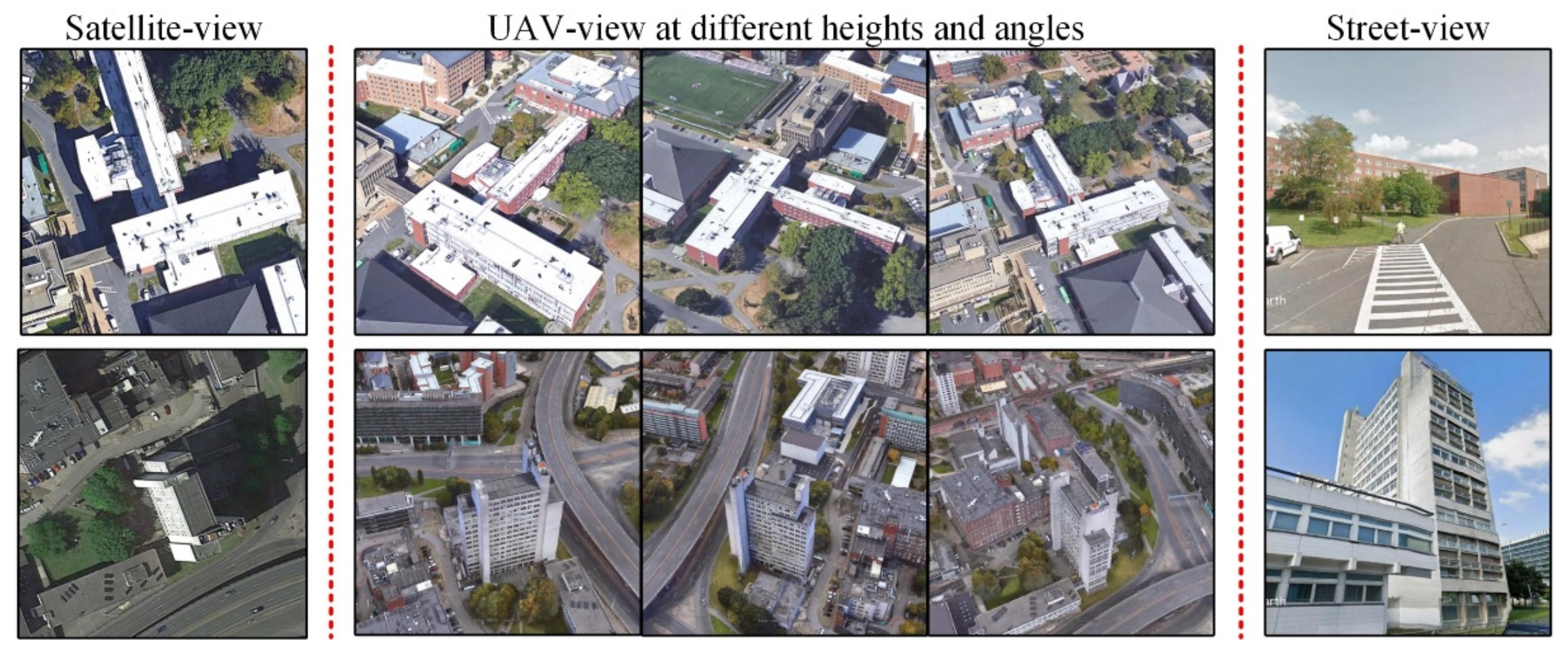
The dataset used in this study is University-1652, released by Zheng et al. [46], which contains 1652 buildings (1652 locations) from 72 universities worldwide. Each building consists of images from three different views, including satellite view, UAV view, and ground view (street view). Additionally, each building in the dataset has only one satellite-view image, 54 UAV-view images from different heights and angles, and one or more ground-view images. Satellite-view images and UAV-view images are adopted in this paper. Please note that the satellite-view images can be satellite images or aerial images because whether a satellite-view image in University-1652 is from a satellite or aircraft is unknown to users. Therefore, considering that the view of the aerial image and the satellite image are close, the “satellite-view image” is used in this study. Besides, the satellite-view image is vertical and the UAV-view image is oblique. Figure 1 shows several images from the three views.
University-1652 was selected as the experimental data for five reasons. First, to the best of our knowledge, it is the only dataset containing both UAV-view and satellite-view images to date. Second, it contains many scenes that are widely distributed and is suitable to be used to train and test models. Third, the target buildings in the images are all ordinary buildings without landmarks, which excludes the influence of special styles on the experiment. Fourth, it has enough image samples for each target building. Fifth, the scales of the satellite-view images and the UAV-view images are similar.
The satellite-view images with geo-tags are from Google Maps. The images of Google Map have high spatial resolutions (from level 18 to level 20, the spatial resolution ranges from 1.07 m to 0.27 m), which have a similar scale to the UAV images. This feature is beneficial to the cross-view image matching of the UAV view and the satellite view. Satellite-view image acquisition is divided into three steps. Firstly, the data owner obtains the metadata (building names and affiliations) of the university building from the websites. Secondly, the data owner obtains the geo-tag (longitude and latitude, in WGS84 coordinate system) of the geometric center of the building on Google Maps based on the metadata. Finally, the data owner acquires the satellite-view images containing the target building and surrounding environment based on the geo-tags.
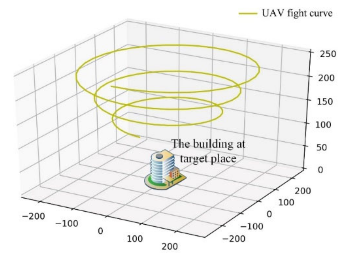
Due to the airspace control and high cost, real UAV-view images of 1652 buildings are difficult to obtain by actual flight. An alternative solution was using the synthetic UAV-view image obtained through simulation to replace the real UAV-view images. The synthetic UAV-view images are obtained by simulating UAV flight based on the 3D building model on Google Earth through the following steps. First, the 3D model of the corresponding building was found according to the name and geo-tag. Second, the UAV simulation video of the 3D building and surrounding environment was obtained according to the pre-set UAV flight path. The schematic diagram of the UAV simulation flight is shown in Figure 2. In order to make the synthesized images contain the multi-angle information of buildings, the UAV flight path is set to a spiral curve. Throughout the simulation process, the flight height is reduced from 256 to 121.5 m. This flight path can make the synthesized image close to the real situation [47,48]. We call synthetic UAV-view image UAV-view images (please note that it is not “UAV images”) because these images were obtained based on the simulated UAV view and are therefore close to the real UAV images. It should be noted that only 1402 buildings out of 1652 buildings have 3D models, and the remaining 250 buildings lack 3D models or street-view images. In addition, real UAV images of ten buildings were additionally provided.
3. Methodology
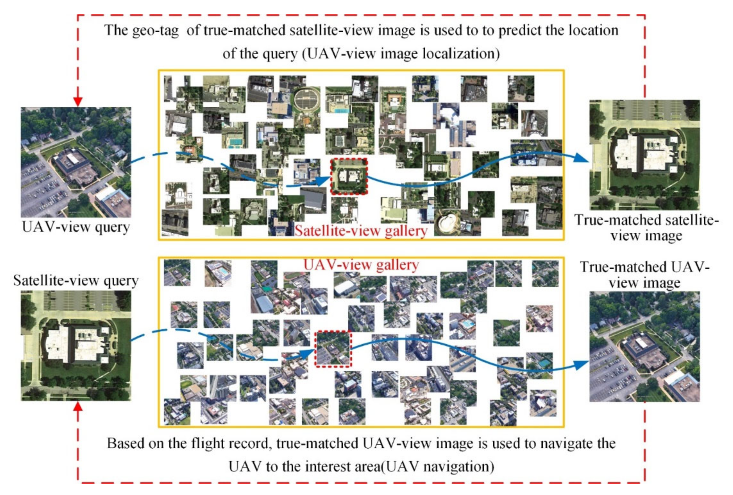
A schematic diagram of the cross-view image matching for UAV-view image localization and UAV navigation is shown in Figure 3. When locating a UAV-view image of a target location, the UAV-view image is first used as a query, and an image of the same target location is then retrieved from the satellite-view gallery (hereinafter referred to as UAV-to-satellite). The geo-tag of the retrieved satellite-view image is used to predict the location of the query image. When navigating the UAV to a target location, a satellite-view image is first used as a query, and an image of the same target location is then retrieved from the UAV-view gallery (hereinafter referred to as satellite-to-UAV). The UAV can recognize where it is by correlating the images it takes with geo-tagged satellite images and is then driven to the target location based on the flight record (the UAV image of the interest area has been acquired by the UAV, and these images are included in the flight record). The key to solving the problems of the UAV-view image localization and UAV navigation is to accurately match the UAV-view image and the satellite-view image.
3.1. Method Framework
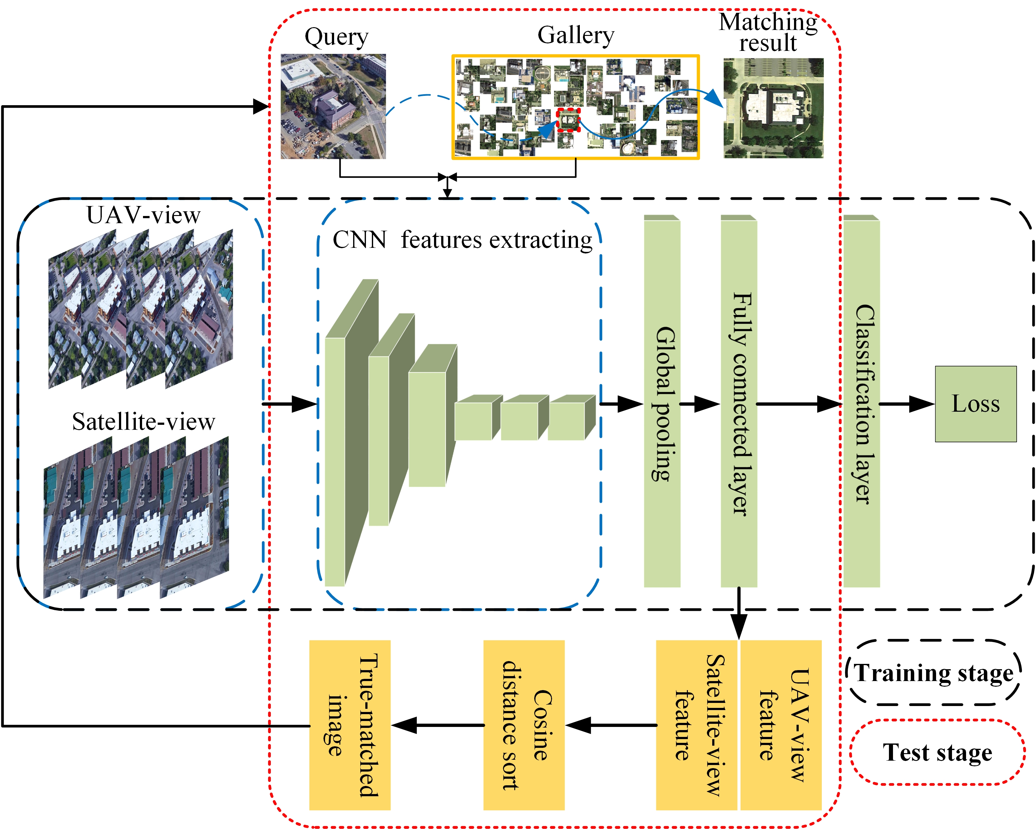
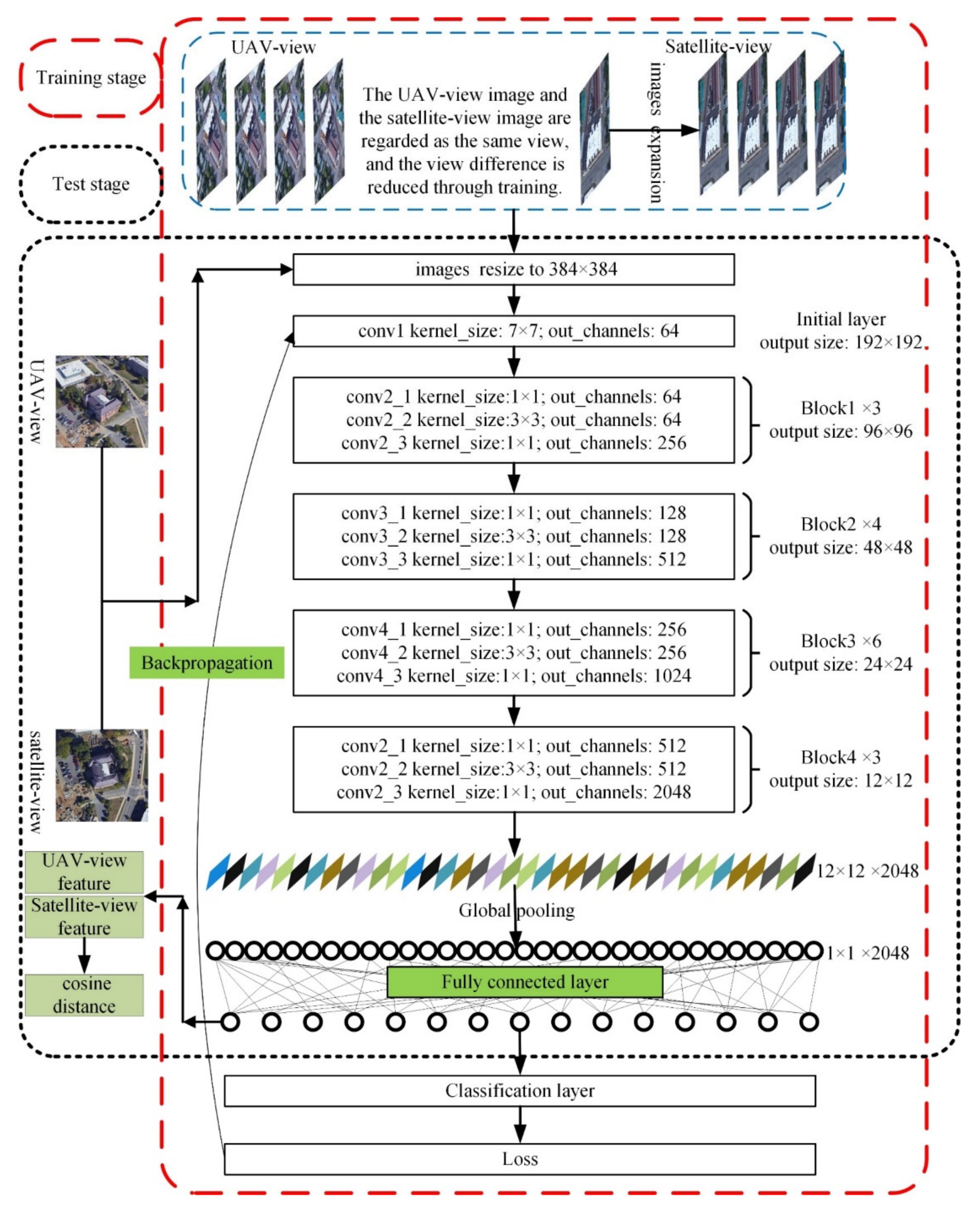
University-1652 has 54 UAV-view images and one satellite-view image of each target building (target location), which means that each target building has enough image samples for training the method. Besides, the UAV-view image and the satellite-view image have certain similarities. Based on the data’s characteristics, we suppose that each target location (target building) is a class. We can regard the cross-view image matching between the UAV-view image and the satellite-view image as a classification task with an unknown number of classes in model training. Based on the above background, a location classification is adopted to propose a cross-view matching method (LCM). The network framework of the LCM is shown in Figure 4. The LCM is divided into two stages: training and test.
A classification framework is built in the training stage. To reduce the difference between the features of the UAV-view image and the satellite-view image, we ignore the view difference between the UAV view and the satellite view and assign the same classification label to the image from the two views at the same target location. In the LCM training, the features of UAV-view images and satellite-view images are mapped to the same feature space through continuous optimization of loss and classification errors. In recent years, the residual network (ResNet) has been widely used in image processing because of its good performance [26,49,50]. The satisfactory classification performance of ResNet-50 on ImageNet has been demonstrated; thus, the pre-trained ResNet-50 model is used as our backbone network to extract image features [51]. The original classification layer in the ResNet-50 network is removed, and then the rest layers in ResNet-50 are used to extract high-level image features. The network architecture is shown in Figure 4. ResNet-50 contains convolutional layers, residual layers, pooling layers, and activation layers. Due to the limitation of figure size, we only show the key convolutional layers, newly added pooling layer, newly added fully connected layer, and newly added classification layer in the figure. He et al. [49] introduced a detailed network structure of ResNet-50. Convolutional layers are usually used to extract the features of the image. The size of the convolution kernels used in ResNet-50 is 3 × 3 and 1 × 1. The convolution formula with a convolution kernel size of 3 × 3 is shown in Equation (1):
where is the input; is the output feature; and bd are the weight of the d-th convolution kernel; c is the number of channels of the input feature map.
The activation layer performs a nonlinear transformation on the output of the convolutional layer to ensure that the model can learn and characterize more complex features. The activation function used in ResNet-50 is ReLU and its formula is:
The residual layer solves the network degradation problem by learning residual features instead of directly learning the underlying features. The residual formula is:
where [O-3]w,h,d is the input features of the residual unit; [O-1]w,h,d is the feature of [O-3]w,h,d after two convolutional layers; and Ow,h,d is the output feature of the residual unit.
Considering that the number of satellite-view images is too small, we expand satellite-view images to a larger number by performing random rotation, cropping, and erasing operations on the original image. The satellite-view image and the UAV-view image are resampled to 384 × 384 and then input to the classification model. After passing through the convolutional layers of ResNet50, the feature dimension of a 384 × 384 × 3 image is 12 × 12 × 2048. Next, we use the global pooling method to change the image feature into a feature vector with a dimension of 2048 [46]. To change the size of the feature vector, a fully connected layer is added after the pooling layer. This fully connected layer can change the image feature size flexibly. After the feature size is changed, it is input to the newly added classification layer to predict the final classification result. Finally, we optimize the loss function according to the classification results and classification labels. During training, the location classification can reduce the difference between the satellite-view image and the UAV-view image, and the location label will make the image with the same label continuously align to the same feature space. The network that we used as the LCM’s baseline model is set as follows: ResNet-50 is used as the backbone network; the output dimension of the fully connected layer size is set to 512; the new classification layer is added after the fully connected layer.
Because the test dataset’s target location does not appear in the training dataset (the location label of the test dataset is not included in the training dataset’s location label), we cannot match the UAV-view image with the satellite-view image by predicting the class in the testing stage. Therefore, the trained classification model cannot be directly used to match the UAV-view image with the satellite-view image. We can only use the image feature in the classification model to implement the cross-view image matching.
In the test stage, the query image (A) from one view (UAV view or satellite view) and the gallery (B) from another view (satellite view or UAV view) are input into the trained classification model. The image features of A and B extracted by the classification model are obtained before the classification layer. Our purpose is to find the image C most relevant to A (at the same location) from B. Therefore, we need an indicator to measure the correlation between A and the images in B. In this framework, the cosine similarity (CS) is adopted to measure the correlation between the features of image A and the features of the image in B [46]. The larger CS means a smaller distance between the two features and a greater correlation between the corresponding images. The CS is determined by Equation (4):
where fA and fB are the feature vectors of A and the images in B; fAi and fBi are the components of feature vectors.
3.2. Loss Function
For the loss function, because the training process is actually a learning process of a classification model, the cross entropy that is often used in multi-classification problems is adopted as the loss function in the model. Cross entropy is mainly used to determine how close the actual output is to the expected output, i.e., the smaller the cross entropy between the network output and the label the better the classification ability of the network. The cross-entropy function of this study is expressed in Equation (5):
where p is a vector that denotes the probability distribution of the sample images with several known classes in the training dataset. For example, when a sample image belongs to the i-th class, the i-th element of p is 1 (i.e., p(xi) = 1) while the other elements are 0; q is a vector that denotes the probability distribution of the predicted class (p(xi) ∈ [0,1]).
3.3. Evaluation Strategy
3.3.1. Test Dataset Split
The LCM is compared with the model of Zheng et al. (hereinafter referred to as the Zheng model), which is the only study using the University-1652 dataset for cross-view image matching to date [46]. For a fair and reliable comparison, this data division in this study is consistent with the Zheng model. Besides, the case in this study, where only the matching of UAV images with satellite images is considered, is also consistent with the Zheng model. The specific data division is shown in Table 1. The 1402 buildings with 3D models were divided into two parts, which were used as a training dataset and query data in the test dataset. To make the test dataset closer to the real situation, the remaining 250 buildings without 3D models or street-view images were used as interference data, which were added to the satellite-view gallery and UAV-view gallery. Therefore, both the UAV-view candidate gallery and the satellite-view candidate gallery contain 951 buildings, while the satellite-view and UAV-view query image contain 701 buildings. Based on this division, the training dataset has a total of 38,555 independent satellite-view images and UAV-view images. Thus, the training dataset is sufficient to train a CNN network. Besides, the training dataset and the test dataset do not have any overlapping buildings and images. This can avoid the case where the network remembers certain buildings in the training dataset and then significantly affects the test results.
3.3.2. Evaluation Indicators
In previous studies on cross-view image matching, the Recall@K is a widely adopted indicator [30,35,46]. If the true-matched image of the query image appears before the (K + 1)-th images in the ranking of the matching result, the value of Recall@K is set to 1. Otherwise, it is set to 0. In the analysis of experimental results, K was set to 1, 5, 10, and 1% of the number of images in the candidate image gallery. The Recall@K of the test dataset is calculated as one of the accuracy evaluation indicators. Recall@K is very sensitive to the position of the first true-matched image appearing in the ranking of the matching result. Therefore, it is suitable for a test dataset that contains only one true-matched image in the candidate gallery. Recall@K is expressed by Equation (6):
where ordertrue-matched is the position of the first true-matched image in the ranking of the matching result.
For satellite-to-UAV, a satellite-view query has 54 true-matched images in the UAV-view gallery. Therefore, to quantitatively evaluate the matching results as comprehensively as possible, the average precision (AP) was used as the other evaluation indicator. The AP is the area under the precision–recall (PR) curve, which considers the position of all true-matched images in the evaluation. The AP of the test dataset is calculated as one of our evaluation indicators. AP is formulated as follows:
where m is the number of true-matched image for a query; Th and Fh are the number of true-matched images and false-matched images before the (i + 1)-th true-matched image in the matching.
4. Experiments Results and Discussions
4.1. Matching Accuracy of LCM’s Baseline Model
In the LCM’s baseline model, the output size of the fully connected layer behind the backbone network is set to 512. Although that the fully connected layer (feature size) is set to different dimensions in Section 4.3, the output size of the fully connected layer in other experiments defaults to 512. The initial learning rates of the backbone network and newly added layers are set to 0.001 and 0.01, respectively. During the training, we gradually decay the learning rate every 80 epochs. The decay rate is 0.1. The dropout rate is set to 0.5. The model optimization method is a stochastic gradient descent with a momentum of 0.9. In addition, all images are resampled to 384 × 384 before being input to the network.
As mentioned above, there is only one satellite-view image of each target location, but there are 54 UAV-view images. Therefore, the satellite-view image accounts for a very low proportion of the training sample (this proportion is 1.8%). Thus, the model has fewer chances to learn feature expressions from satellite-view images during the training. The model that is trained based on the training dataset with unbalanced samples may not fully express the features of the satellite-view image, which may decrease the matching accuracy. The number of satellite-view images of a target location has been expanded from 1 to 54 by generating new satellite-view images through randomly rotating, cropping, and erasing. Through the strategy above, the target location of the training dataset has 54 UAV-view images and 54 satellite-view images.
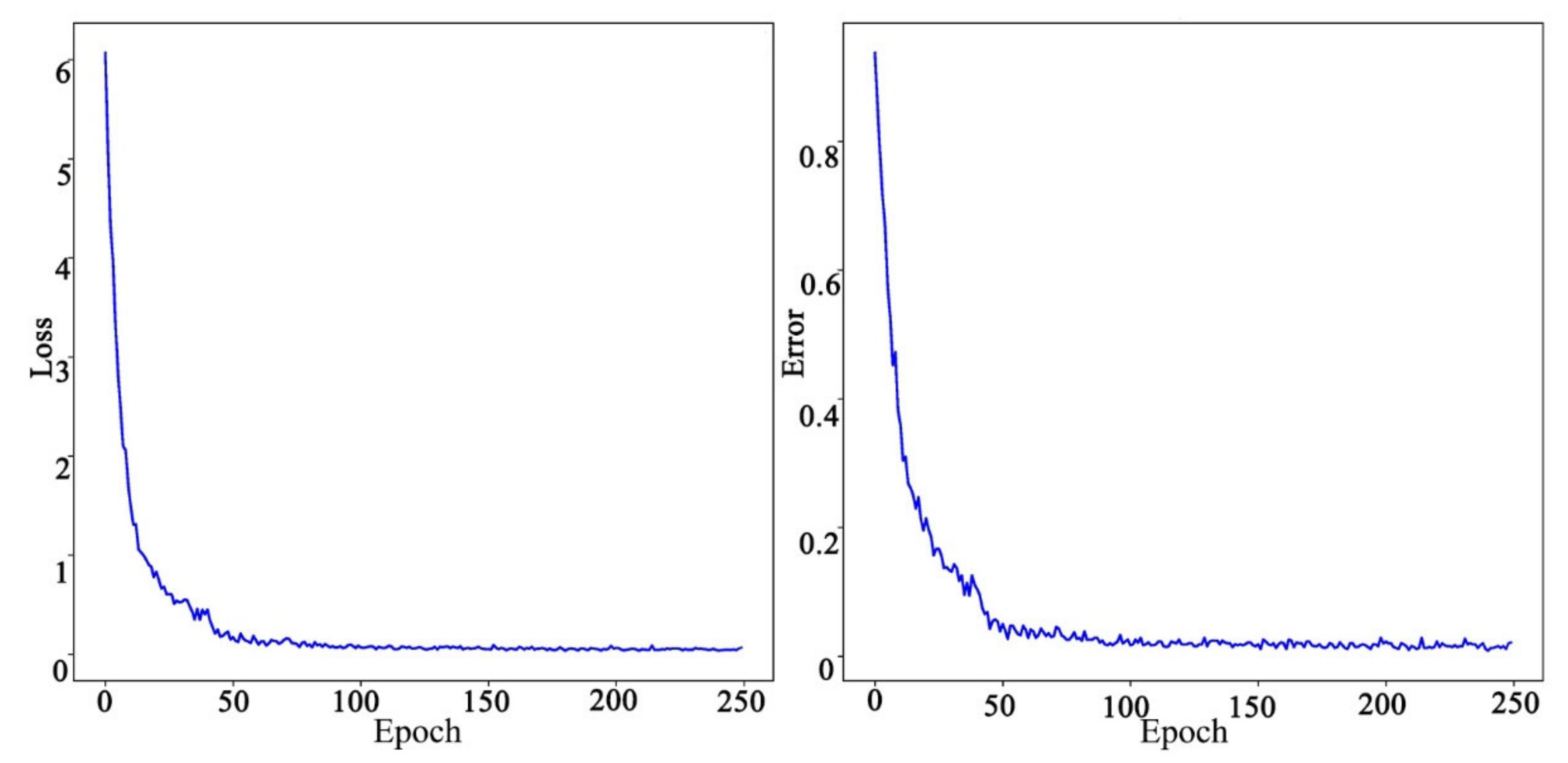
The variations of the two significant parameters, i.e., loss and classification error, during the training process are shown in Figure 5. Loss is the average value of the cross entropy; classification error is the average probability of the image being misclassified. Because the LCM is not a classification model, the loss and classification error in the test dataset cannot be calculated. To enable the model to learn the optimal parameters, 250 epochs are used in this study. The smaller loss and classification error means that the model can more classify satellite-view images and UAV-view images of the same target location into one class accurately, which suggests that the model can map image features from two views to the same space. Besides, if a target building is included in the training dataset, the method is able to classify images of the building with the same origin (both UAV or both satellite) into the same class. If a target building is not included in the training dataset, the method will classify images of the building with the same origin (both UAV or both satellite) into the same class by relying on the feature similarity between the image of the target building and the image in the relevant gallery. After 50 epochs, loss and classification errors are quickly reduced to 0.198 and 3.56%, respectively. After 100 epochs, loss and classification errors tend to converge. After 250 epochs (approximately 58 min), loss and classification error were reduced to 0.045 and 1.16%, respectively. These results show that LCM model has the advantages of fast convergence and short training time. In addition, the results also indicate that inputting the satellite view and UAV view of the same target location to the classification model without differences performs well. In other words, the proposed LCM can map image features from two different views to the same space through classification.
The comparison results of the LCM’s baseline model and Zheng model are shown in Table 2. When single satellite-view images are used as the query, the Recall@1, Recall@10, and AP of the LCM are higher by 5.42%, 6.65%, and 5.93% than the Zheng model, respectively. When single UAV-view images are used as the query, the Recall@1, Recall@10, and AP of our model are also higher by 8.16%, 4.79%, and 7.69% than those of the Zheng model, respectively. Overall, the LCM can more effectively extract the image features of the two views, thereby improving the matching accuracy. In addition, the Recall@1 and AP in UAV-to-satellite are more significantly improved than satellite-to-UAV.
At present, the probability that the first image in the ranking of the matching result is the exact true-matched image of the query image cannot be 100%. When the first image in the ranking of the matching result is not the true-matched image, we need to manually find the true-matched image of the query image according to the ranking of the matching results. Table 2 shows that, for the LCM, the probability of finding the true-matched image of the query in the top ten of the ranking of the matching result is higher than 90%. This means that although the LCM cannot automatically give the correct location of the query in some cases, it still allows us to find the true-matched image and significantly improves the accuracy of the matching with high efficiency.
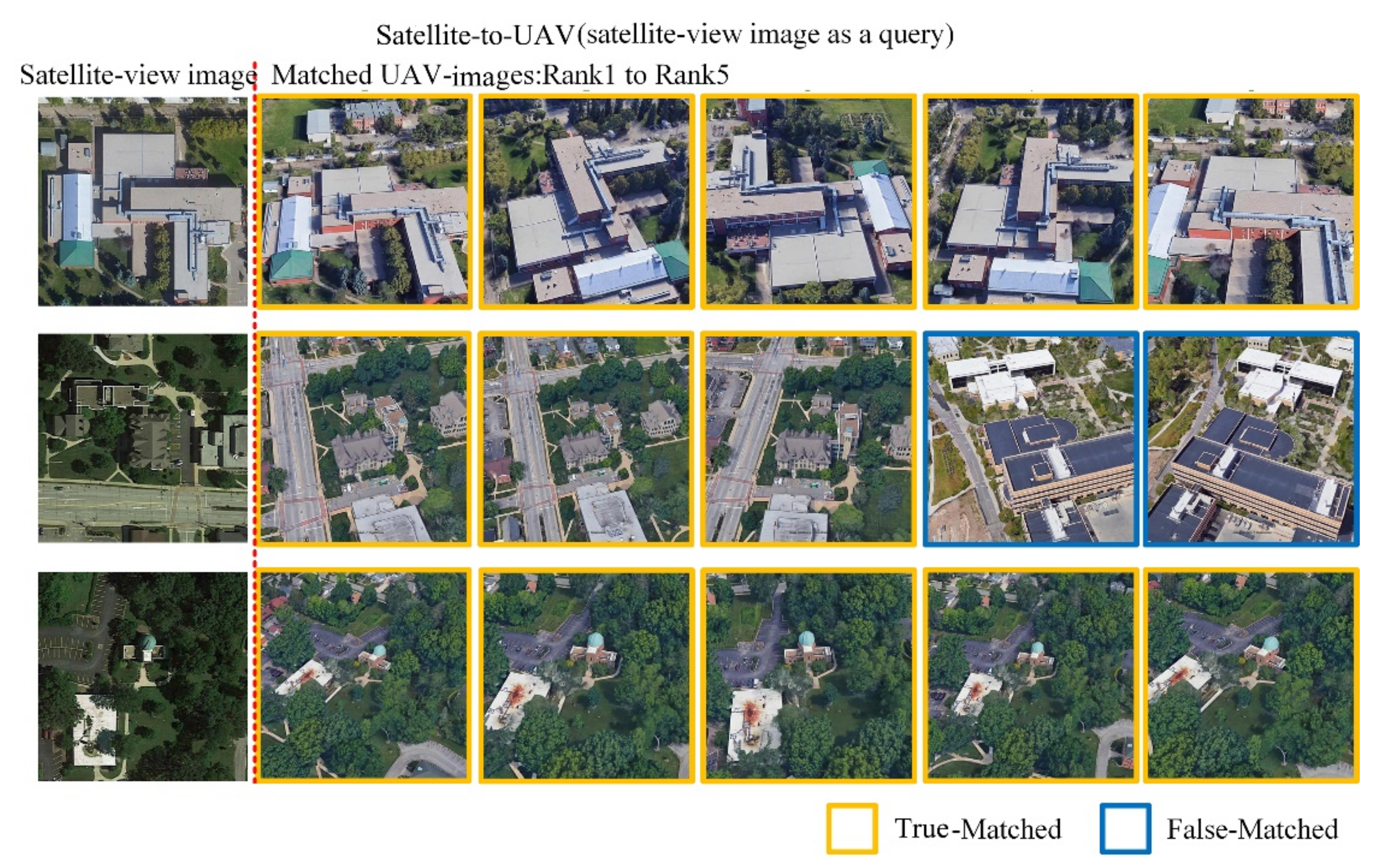
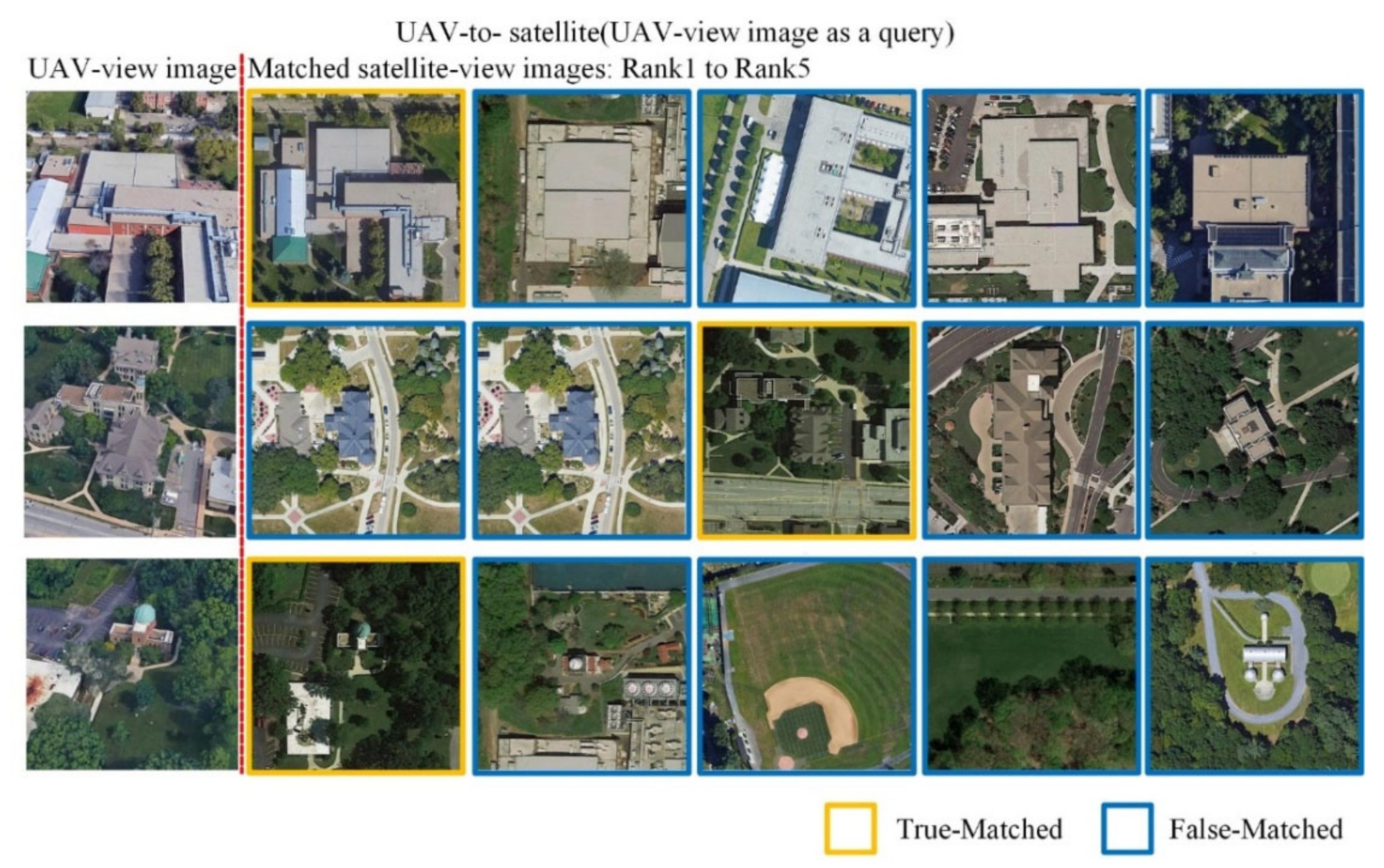
To further quantitatively evaluate the LCM’s baseline model, the visualization results of two cases are shown in Figure 6 and Figure 7. For each location (a line of images), the image on the left of the red line in the figure is the query image, and the five images on the right of the red line are the top five images in the ranking of the matching result.
For satellite-to-UAV (Figure 6), the LCM baseline model can find the images at the same target location as the query image in the UAV-view gallery. For satellite-to-UAV, Figure 6 shows that the top five images in the ranking of matching result have multiple true-matched images. The reason is that there are 54 images that can be correctly matched with each satellite image in the UAV-view gallery. For UAV-to-satellite, Figure 7 shows that the top five images in the ranking of the matching result have only one true-matched image. The reason is that there is only one image that can be correctly matched with each UAV image in the satellite-view gallery. A closer look at Figure 7 shows that these false-matched images have similar structures and features to the query images. This indicates that the LCM’s baseline model can effectively capture images with similar characteristics to the query image, and therefore benefit the cross-view image matching.
To further compare and analyze the influence of different types and depths of CNNs on the LCM, we used ResNet-50, VGG-16, and DensNet-121 as the LCM’s backbone network [52,53]. The matching accuracies of the LCM using these three different backbone networks are shown in Table 3. VGG-16 has the worst performance among the three backbone networks. For satellite-to-UAV (UAV-to-satellite), the Recall@1, Recall@5, Recall@10, and AP of the LCM are lower by 11.84% (18.46%), 7.31% (12.24%), 7.01% (9.67%), and 17.55% (11.37%), respectively, when VGG-16 rather than ResNet-50 is used as the backbone network. The possible reason is that the VGG-16 network has fewer layers, resulting in its weaker ability of feature expression than ResNet-50. The accuracy of DensNet-121 is slightly lower than ResNet-50. For satellite-to-UAV (UAV-to-satellite), the Recall@1, Recall@5, Recall@10, and AP of LCM are lower by 2.14% (1.64%), 12.24% (0.3%), 0.59% (1.15%), and 6.12% (1.33%), respectively, when the DensNet-121 rather than ResNet-50 is used as the backbone network. Although DensNet-121 has more network layers, it does not perform better than ResNet-50 in this task. The possible reason is that the features extracted by DensNet-121 are not suitable for the LCM. This conclusion shows that the networks that are deeper and more complex than ResNet-50 cannot improve the accuracy of the LCM’s baseline. ResNet-50 has the best and most stable performance in the three backbone networks for the LCM’s baseline. In the following experiments, if we do not specify otherwise, ResNet-50 will serve as our backbone network.
4.2. Influence of Satellite Image Expansion on the Matching Accuracy
In the LCM’s baseline model, we expanded the number of satellite-view images to 54 (the same number as the UAV-view images) of a target location. Will different numbers of satellite-view images affect matching accuracy? Do 54 satellite images of each target location as a training dataset have the best matching accuracy for the LCM? To answer the above questions, we conducted the following comparative experiment. Random rotation, cropping, and erasing operations were performed on a satellite-view image of each target location (it is consistent with the satellite-view image expansion method in the LCM’s baseline model). In this way, new satellite-view images were generated by increasing the number of images associated with each target location in several ways, namely to 1, 3, 9, 18, 27, 54, and 81 images per target. These training datasets containing different numbers of satellite-view images of a target location were used to train models. The matching accuracies of these models on the test dataset were also tested, and the test results are shown in Table 4.
According to Table 4, it is clear that when we do not expand the number of the satellite-view images (namely, only using one satellite image of each target location), the LCM model has the lowest matching accuracy. With the increase in satellite-view image samples, Recall@K and AP gradually increase and the upward trend gradually slows down. When the numbers of satellite-view images and the UAV-view images of a target location are the same, Recall@K and AP reach their maximum values. When the number of satellite-view images at a target location increases from 1 to 54 for satellite-to-UAV, Recall@1, Recall@5, Recall@10, and AP increase by 9.99%, 8.60%, 8.31%, and 6.94%, respectively; for UAV-to-satellite, Recall@1, Recall@5, Recall@10, and AP increase by 7.04%, 5.65%, 5.09%, and 6.71%, respectively. When the number of satellite-view images of a target location increases from 54 to 81, Recall@K and AP show a slight decrease. For satellite-to-UAV, Recall@1, Recall@5, Recall@10, and AP decrease by 0.29%, 0.46%, 0.59%, and 1.29%, respectively; for UAV-to-satellite, Recall@1, Recall@5, Recall@10, and AP decrease by 2.03%, 1.24%, 1.60%, and 1.89%. The possible reason for this phenomenon is the imbalance of the image samples of the two views. When there are more image samples of view A than of view B, the feature expressed by the classification model will be closer to the feature space of view A.
In general, the Recall@K of satellite-to-UAV is higher than that of UAV-to-satellite, especially Recall@1. This phenomenon can be attributed to the difference in the number of true-matched images of the two views at the same target location. For satellite-to-UAV, when we use a satellite-view image as the query, there are 54 true-matched images in the UAV-view gallery. In this case, if any of the 54 true-matched images appear before the (K + 1)-th images in the ranking of the matching result, we can set Recall@K to 1. For UAV-to-satellite, when we use a UAV-view image as the query, there is only one true-matched image in the satellite-view gallery. In this case, we can set Recall@K to 1 only if this true-matched satellite-view image appears before the (K + 1)-th images in the ranking of the matching result. Therefore, the Recall@K of satellite-to-UAV is expected to be higher than the Recall@K of UAV-to-satellite in the same test dataset.
According to the above comparative experiment, it is evident that when the number of the satellite-view images at a target location is expanded to 54 (the number is the same as the number of UAV-view images), the trained model will show the best performance.
4.3. Matching Accuracy of Different Feature Sizes
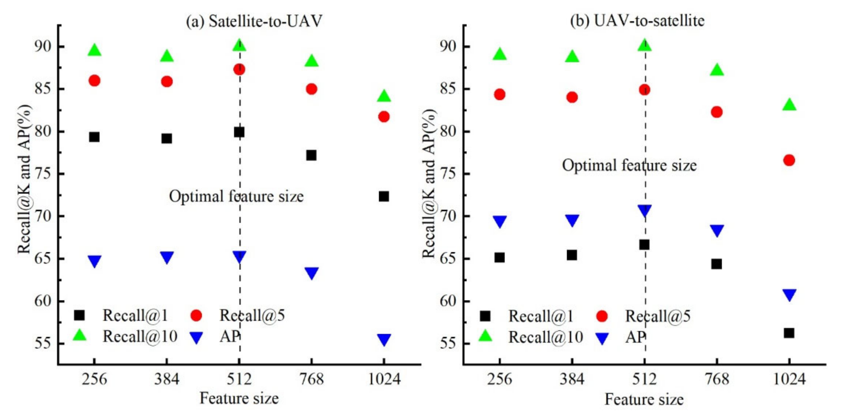
In Section 4.1, the size of the feature vector we used to calculate the CS is 512 dimensions (the output size of the fully connected layer after the backbone network is 512 dimensions). Thus, we want to explore the following questions: does the size of the feature vector used to calculate the CS have an effect on the experimental results? To answer the question, we embedded the fully connected layers with different output sizes into the LCM and trained them. Finally, the obtained models were used to test. Feature vectors of five sizes of 256, 384, 512, 768, and 1024 are selected for comparison. Figure 8 shows the relationship between the cross-view matching accuracy and the feature size.
As shown in Figure 8, we cannot find the phenomenon that a larger feature vector size can lead to a higher Recall@K and AP. The relationship between the matching accuracy and the feature size can be divided into two cases. The first case is when the feature size ranges from 256 to 512, Recall@K and the AP become larger as the feature size increases. When the feature size is 512, the LCM has an optimal matching accuracy. However, the matching accuracy exhibits relatively low variations in this case. For satellite-to-UAV, Recall@1, Recall@5, Recall@10, and AP increase by 0.57%, 1.32%, 0.59%, and 0.51%, respectively; for UAV-to-satellite, Recall@1, Recall@5, Recall@10, and AP increase by 1.51%, 0.57%, 1.07%, and 1.29%, respectively. In the second case, when the feature size ranges from 512 to 1024, Recall@K and AP decrease as the feature size increases. When the feature size is set to 1024, the lowest matching accuracy is shown. Compared with the first case, the matching accuracy varies relatively more rapidly in this case. For satellite-to-UAV, Recall@1, Recall@5, Recall@10, and AP decrease by 7.56%, 5.60%, 6.01%, and 9.77%, respectively; for UAV-to-satellite, Recall@1, Recall@5, Recall@10, and AP decrease by approximately 10.42%, 8.32%, 7.01%, and 9.91%, respectively. Obviously, 512 is the optimal feature size. This is why we used this feature size in the LCM model (see Section 4.1).
4.4. Matching Accuracy of Multiple Queries
In previous matching experiments, a single UAV-view image was used as a query for UAV-to-satellite. In University-1652, the synthesized UAV-view images were viewed obliquely all around the target building; thus, it is difficult for a single UAV-view query to provide comprehensive information about the target building. Fortunately, University-1652 provides synthetic UAV images at different heights and angles for each target building. These UAV-view images from different viewpoints can provide comprehensive information and characteristics of each target building. This means that for UAV-to-satellite, we can use multiple UAV-view images as a query at the same time. To explore whether multiple queries can improve the matching accuracy of UAV-to-satellite, all synthetic UAV images of a target building were used as the query, and then the image of the same location as the query in the satellite-view gallery was retrieved.
To facilitate the measurement of the correlation between the multi-query images and the image in the gallery, the feature of multiple queries is set as the mean value of the single image feature of a target building. In our experiment, the features of 54 UAV-view images were averaged and used as the feature of multiple queries. The test accuracy of multiple queries is shown in Table 5. From the table, it is clear that compared with the original single query, the matching accuracy of multiple queries can be improved by about 10% in both Recall@1 and AP. Besides, Recall@5 and Recall@10 are also significantly improved. We also compared the matching results of multiple queries of the LCM with the results of the Zheng model. The comparison results show that the LCM performs better than the Zheng model when using multiple queries: Recall@1, Recall@5, Recall@10, and AP are increased by 8.56%, 4.57%, 3.42%, and 7.91%, respectively.
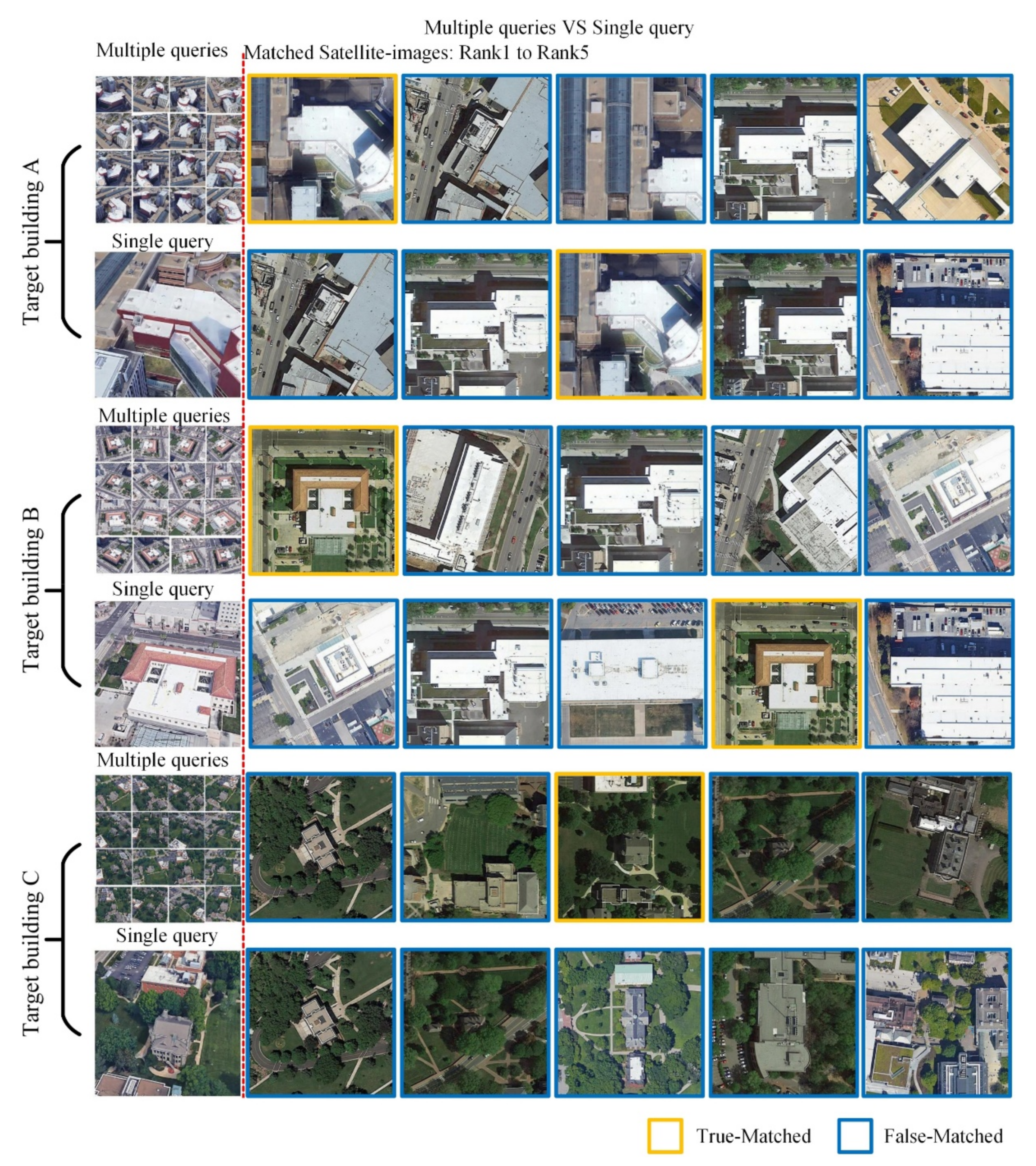
To investigate the effectiveness of using multiple queries more clearly, we visualized the matching results of multiple queries and a single query of three target buildings (targets A, B, and C). The visual details are shown in Figure 9. For the target buildings A and B, the true-matched satellite-view images appeared in the third and fourth position in the ranking of the matching results when we use a single query. When we use multiple queries, the true-matched satellite-view images all appeared in the first position in the ranking of the matching results. For target building C, the true-matched satellite-view image does not appear in the top five in the ranking of the matching results. When we use multiple queries, the true-matched satellite-view image appeared in the third position in the ranking of the matching results. These results demonstrate that multiple queries can indeed improve the matching accuracy of UAV-to-satellite when we use the LCM. For satellite-to-UAV, because only one satellite-view image can be used as a query of the target location, the experiments of multiple queries cannot be conducted.
4.5. Matching Result of the Real UAV-View Image
In previous experiments, the UAV-view images used in the training and testing of the model were all synthetic UAV-view images based on 3D buildings. To further evaluate the performance of the LCM on real UAV-view images, we conducted the following two experiments. Firstly, we used the real UAV-view query to match the synthetic UAV-view images of the same location (hereinafter referred to as RUAV-to-SUAV). Secondly, we used real UAV-view queries to match the satellite-view images of the same location (hereinafter referred to as RUAV-to-Sat). Real UAV-view images are also provided by University-1652. Due to the restrictions of airspace control and privacy protection policies, there are only 10 real UAV-view images; therefore, we only selected a few target buildings with real UAV-view images for experiments. Because there are few real UAV-view images that can be used as queries, Recall@K and AP were not employed as quantitative evaluation indicators here. We only show the visual matching results of the two experiments.
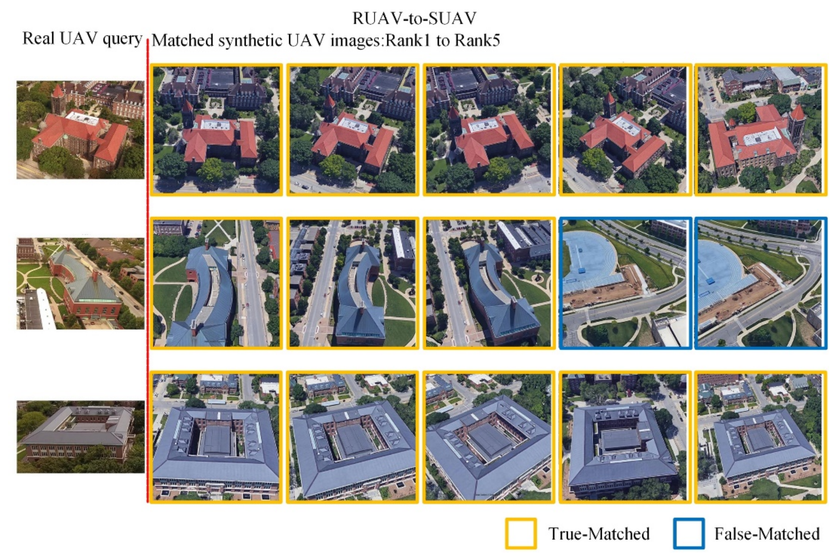
Figure 10 shows the matching results of RUAV-to-SUAV. When real UAV-view images are used as the query, the LCM can accurately match the images of the same location in the synthetic UAV-view gallery. This result not only shows that the LCM is effective in the feature expression of the real UAV-view images but also shows that the synthetic UAV-view images in University-1652 are close to the real scenes.
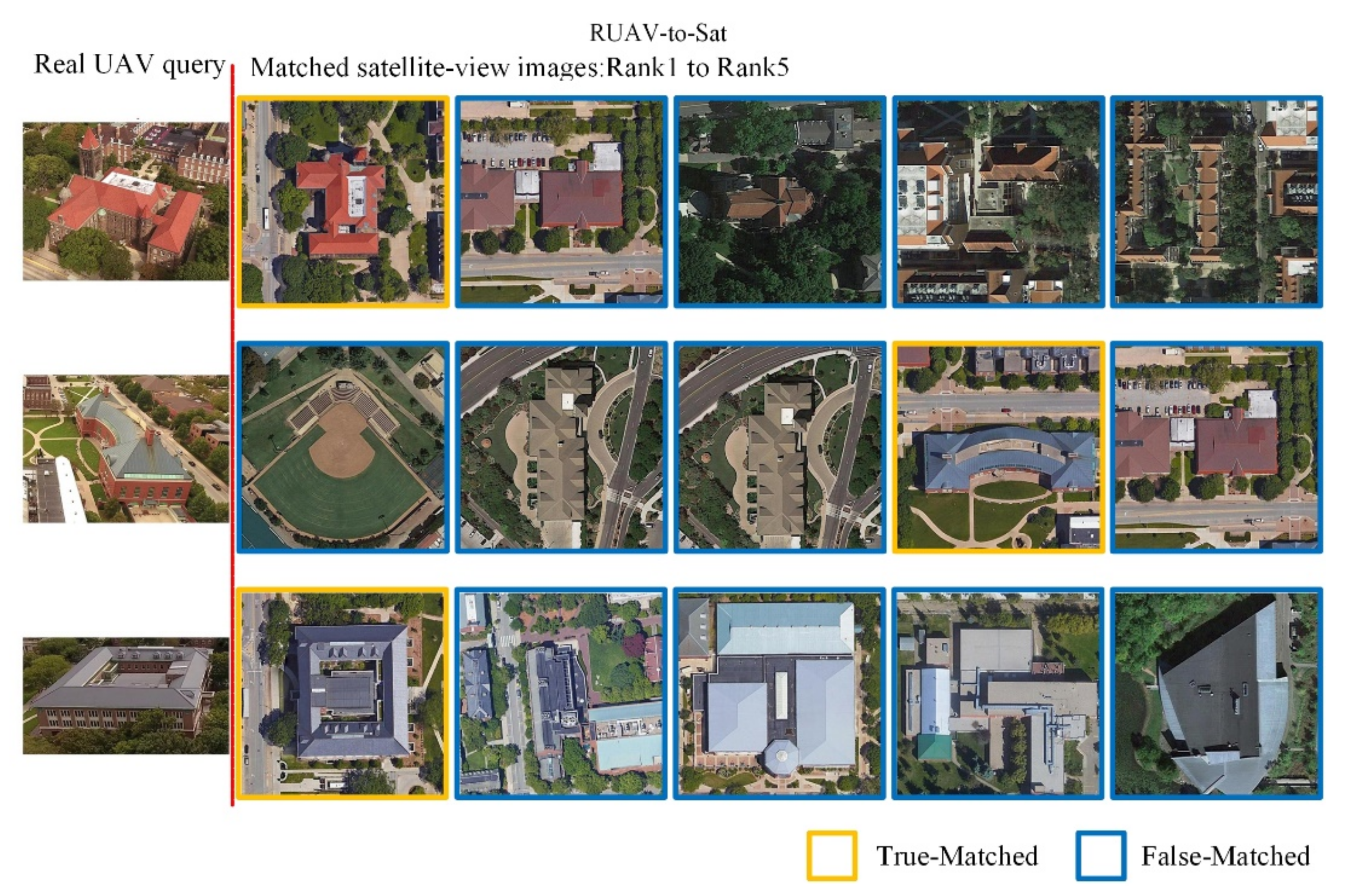
The matching results of RUAV-to-Sat are shown in Figure 11. The performance of the experimental results is consistent with the one in which we use the synthetic UAV-view image as a query to match the satellite-view image. The LCM can successfully match the real UAV-view images with the satellite-view images. The false-matched satellite-view image and the true-matched satellite-view image have similar structural and color features. It further shows that the LCM trained based on the synthetic UAV-view images also has a good matching performance in the real images.
Because the University-1652 dataset does not provide the height and angle of the UAV-view images, we cannot obtain the scale differences of different UAV-view images and the scale differences between satellite-view and UAV-view images. In addition, the scale of different UAV-view images from different heights and the scale of satellite-view and UAV-view images used in this study are close. Therefore, the influence of the scale difference was not considered. However, the scale difference is important for cross-view image matching. Therefore, we will consider the issue in the practical application of the method in future studies.
5. Conclusions
UAV technology has been developed rapidly in recent years. The localization of UAV images without geo-tags and UAV navigation without geographic coordinates are crucial for users. Cross-view image matching is an effective method to realize UAV-view image localization and UAV navigation. However, the algorithms of cross-view image matching between the UAV view and the satellite view are still in their beginning stage, and the matching accuracy is expected to be further improved when applied in real situations.
This study explores the problem of cross-view image matching between UAV-view images and satellite-view images. Based on University-1652, a cross-view image matching method (LCM) for UAV-view image localization and UAV navigation was proposed. The LCM is based on the idea of classification and has the advantages of fast training and high matching accuracy. There are two findings from the experiment: (1) expanding the satellite-view image can improve the sample imbalance between the satellite-view image and the UAV-view image, thereby improving the matching accuracy of the LCM; (2) appropriate feature dimensions and multiple queries can significantly improve the matching accuracy of the LCM. In addition, the LCM trained based on synthetic UAV-view images also shows a good performance in matching real UAV-view images and satellite-view images. Compared with one previous study, various accuracy indicators of matching the UAV-view image and the satellite-view image based on the LCM have been improved by about 5–10%. Therefore, the LCM can better serve the UAV-view image localization and UAV navigation. In the future, we will continue to explore how to further improve the matching accuracy of UAV-view images and satellite-view images and how to use UAV images as an intermediate bridge to improve the matching accuracy of general street-view images and satellite-view images. In addition, please note that the UAV height in University-1652 is unrealistic for practical applications due to airspace regulations. Therefore, in the future, we will consider this issue and simulate the UAV images at a lower flight height.
Author Contributions
Conceptualization, L.D. and J.Z.; methodology, L.D. and L.M.; software, Z.L. and L.D.; investigation, Z.L. and L.D.; resources, J.Z.; data curation, L.D.; writing—original draft preparation, L.D.; writing—review and editing, J.Z. and L.D.; visualization, L.D. and L.M.; supervision, J.Z.; project administration, J.Z.; funding acquisition, J.Z. All authors have read and agreed to the published version of the manuscript.
Funding
This work was supported by the Sichuan Province Science and Technology Plan Applied Basic Research Project (grant number: 2019YJ0205), and by the Fundamental Research Funds for the Central Universities of China (grant number: ZYGX2019J069).
Institutional Review Board Statement
Not applicable.
Informed Consent Statement
Not applicable.
Data Availability Statement
Data sharing not applicable.
Acknowledgments
The authors would like to thank Zheng Zhedong from the Reler laboratory, University of Technology Sydney for providing the Universty-1652 dataset and open source code.
Conflicts of Interest
The authors declare no conflict of interest.
References
- Mesas-Carrascosa, F.J.; Notario-García, M.D.; de Larriva, J.E.M.; de la Orden, M.S.; Porras, A.G.-F. Validation of Measurements of Land Plot Area Using UAV Imagery. Int. J. Appl. Earth Obs. Geoinf. 2014, 33, 270–279. [Google Scholar] [CrossRef]
- Wu, Z.; Ni, M.; Hu, Z.; Wang, J.; Li, Q.; Wu, G. Mapping Invasive Plant with UAV-Derived 3D Mesh Model in Mountain Area—A Case Study in Shenzhen Coast, China. Int. J. Appl. Earth Obs. Geoinf. 2019, 77, 129–139. [Google Scholar] [CrossRef]
- Deng, L.; Mao, Z.; Li, X.; Hu, Z.; Duan, F.; Yan, Y. UAV-Based Multispectral Remote Sensing for Precision Agriculture: A Comparison between Different Cameras. ISPRS J. Photogramm. Remote Sens. 2018, 146, 124–136. [Google Scholar] [CrossRef]
- Alexander, C.; Korstjens, A.H.; Hankinson, E.; Usher, G.; Harrison, N.; Nowak, M.G.; Abdullah, A.; Wich, S.A.; Hill, R.A. Locating Emergent Trees in a Tropical Rainforest Using Data from an Unmanned Aerial Vehicle (UAV). Int. J. Appl. Earth Obs. Geoinf. 2018, 72, 86–90. [Google Scholar] [CrossRef]
- Dehkordi, R.H.; Denis, A.; Fouche, J.; Burgeon, V.; Cornelis, J.T.; Tychon, B.; Gomez, E.P.; Meersmans, J. Remotely-Sensed Assessment of the Impact of Century-Old Biochar on Chicory Crop Growth Using High-Resolution UAV-Based Imagery. Int. J. Appl. Earth Obs. Geoinf. 2020, 91, 102147. [Google Scholar] [CrossRef]
- Hamylton, S.M.; Morris, R.H.; Carvalho, R.C.; Roder, N.; Barlow, P.; Mills, K.; Wang, L. Evaluating Techniques for Mapping Island Vegetation from Unmanned Aerial Vehicle (UAV) Images: Pixel Classification, Visual Interpretation and Machine Learning Approaches. Int. J. Appl. Earth Obs. Geoinf. 2020, 89, 102085. [Google Scholar] [CrossRef]
- Ji, L.; Zhu, L.; Wang, L.; Xi, Y.; Yu, K.; Geng, X. FastVGBS: A Fast Version of the Volume-Gradient-Based Band Selection Method for Hyperspectral Imagery. IEEE Geosci. Remote Sens. Lett. 2020, 1–4. [Google Scholar] [CrossRef]
- Ammour, N.; Alhichri, H.; Bazi, Y.; Benjdira, B.; Alajlan, N.; Zuair, M. Deep Learning Approach for Car Detection in UAV Imagery. Remote Sens. 2017, 9, 312. [Google Scholar] [CrossRef] [Green Version]
- Ferrer-González, E.; Agüera-Vega, F.; Carvajal-Ramírez, F.; Martínez-Carricondo, P. UAV Photogrammetry Accuracy Assessment for Corridor Mapping Based on the Number and Distribution of Ground Control Points. Remote Sens. 2020, 12, 2447. [Google Scholar] [CrossRef]
- Lin, Y.-C.; Cheng, Y.-T.; Zhou, T.; Ravi, R.; Hasheminasab, S.M.; Flatt, J.E.; Troy, C.; Habib, A. Evaluation of UAV LiDAR for Mapping Coastal Environments. Remote Sens. 2019, 11, 2893. [Google Scholar] [CrossRef] [Green Version]
- Yan, Y.; Deng, L.; Liu, X.; Zhu, L. Application of UAV-Based Multi-Angle Hyperspectral Remote Sensing in Fine Vegetation Classification. Remote Sens. 2019, 11, 2753. [Google Scholar] [CrossRef] [Green Version]
- Liu, W.; Yang, M.; Xie, M.; Guo, Z.; Li, E.; Zhang, L.; Pei, T.; Wang, D. Accurate Building Extraction from Fused DSM and UAV Images Using a Chain Fully Convolutional Neural Network. Remote Sens. 2019, 11, 2912. [Google Scholar] [CrossRef] [Green Version]
- Hays, J.; Efros, A.A. IM2GPS: Estimating geographic information from a single image. In Proceedings of the 2008 IEEE Conference on Computer Vision and Pattern Recognition, Anchorage, AK, USA, 23–28 June 2008; pp. 1–8. [Google Scholar]
- Sattler, T.; Havlena, M.; Schindler, K.; Pollefeys, M. Large-scale location recognition and the geometric burstiness problem. In Proceedings of the IEEE Conference on Computer Vision and Pattern Recognition, Las Vegas, NV, USA, 27–30 June 2016; pp. 1582–1590. [Google Scholar]
- Vo, N.; Jacobs, N.; Hays, J. Revisiting im2gps in the deep learning era. In Proceedings of the IEEE International Conference on Computer Vision, Venice, Italy, 22–29 October 2017; pp. 2621–2630. [Google Scholar]
- Zamir, A.R.; Shah, M. Image geo-localization based on multiplenearest neighbor feature matching usinggeneralized graphs. IEEE Trans. Pattern Anal. Mach. Intell. 2014, 36, 1546–1558. [Google Scholar] [CrossRef]
- Fu, K.; Chang, Z.; Zhang, Y.; Xu, G.; Zhang, K.; Sun, X. Rotation-aware and multi-scale convolutional neural network for object detection in remote sensing images. ISPRS J. Photogramm. Remote Sens. 2020, 161, 294–308. [Google Scholar] [CrossRef]
- Li, K.; Wan, G.; Cheng, G.; Meng, L.; Han, J. Object Detection in Optical Remote Sensing Images: A Survey and a New Benchmark. ISPRS J. Photogramm. Remote Sens. 2020, 159, 296–307. [Google Scholar] [CrossRef]
- Mao, T.; Tang, H.; Huang, W. Unsupervised Classification of Multispectral Images Embedded With a Segmentation of Panchromatic Images Using Localized Clusters. IEEE Trans. Geosci. Remote Sens. 2019, 57, 8732–8744. [Google Scholar] [CrossRef]
- Mi, L.; Chen, Z. Superpixel-Enhanced Deep Neural Forest for Remote Sensing Image Semantic Segmentation. ISPRS J. Photogramm. Remote Sens. 2020, 159, 140–152. [Google Scholar] [CrossRef]
- Zhang, X.; Xiao, P.; Feng, X. Object-Specific Optimization of Hierarchical Multiscale Segmentations for High-Spatial Resolution Remote Sensing Images. ISPRS J. Photogramm. Remote Sens. 2020, 159, 308–321. [Google Scholar] [CrossRef]
- Sedona, R.; Cavallaro, G.; Jitsev, J.; Strube, A.; Riedel, M.; Benediktsson, J.A. Remote Sensing Big Data Classification with High Performance Distributed Deep Learning. Remote Sens. 2019, 11, 3056. [Google Scholar] [CrossRef] [Green Version]
- Lv, Y.; Zhang, X.; Xiong, W.; Cui, Y.; Cai, M. An End-to-End Local-Global-Fusion Feature Extraction Network for Remote Sensing Image Scene Classification. Remote Sens. 2019, 11, 3006. [Google Scholar] [CrossRef] [Green Version]
- Peng, D.; Zhang, Y.; Guan, H. End-to-End Change Detection for High Resolution Satellite Images Using Improved Unet++. Remote Sens. 2019, 11, 1382. [Google Scholar] [CrossRef] [Green Version]
- Chang, Y.-L.; Anagaw, A.; Chang, L.; Wang, Y.C.; Hsiao, C.-Y.; Lee, W.-H. Ship Detection Based on YOLOv2 for SAR Imagery. Remote Sens. 2019, 11, 786. [Google Scholar] [CrossRef] [Green Version]
- Meng, L.; Peng, Z.; Zhou, J.; Zhang, J.; Lu, Z.; Baumann, A.; Du, Y. Real-Time Detection of Ground Objects Based on Unmanned Aerial Vehicle Remote Sensing with Deep Learning: Application in Excavator Detection for Pipeline Safety. Remote Sens. 2020, 12, 182. [Google Scholar] [CrossRef] [Green Version]
- Lin, T.-Y.; Cui, Y.; Belongie, S.; Hays, J. Learning deep representations for ground-to-aerial geolocalization. In Proceedings of the IEEE Conference on Computer Vision and Pattern Recognition, Boston, MA, USA, 7–12 June 2015; pp. 5007–5015. [Google Scholar]
- Tian, Y.; Chen, C.; Shah, M. Cross-view image matching for geo-localization in urban environments. In Proceedings of the IEEE Conference on Computer Vision and Pattern Recognition, Honolulu, HI, USA, 21–26 July 2017; pp. 3608–3616. [Google Scholar]
- Zhai, M.; Bessinger, Z.; Workman, S.; Jacobs, N. Predicting ground-level scene layout from aerial imagery. In Proceedings of the IEEE Conference on Computer Vision and Pattern Recognition, Honolulu, HI, USA, 21–26 July 2017; pp. 867–875. [Google Scholar]
- Liu, L.; Li, H. Lending orientation to neural networks for cross-view geo-localization. In Proceedings of the 2019 IEEE/CVF Conference on Computer Vision and Pattern Recognition (CVPR), Long Beach, CA, USA, 15–20 June 2019. [Google Scholar]
- Bansal, M.; Daniilidis, K.; Sawhney, H. Ultra-wide baseline facade matching for geo-localization. In Proceedings of the European Conference on Computer Vision, Florence, Italy, 7–13 October 2012; pp. 175–186. [Google Scholar]
- Lin, T.-Y.; Belongie, S.; Hays, J. Cross-view image geolocalization. In Proceedings of the IEEE Conference on Computer Vision and Pattern Recognition, Portland, OR, USA, 23–28 June 2013; pp. 891–898. [Google Scholar]
- Shan, Q.; Wu, C.; Curless, B.; Furukawa, Y.; Hernandez, C.; Seitz, S.M. Accurate geo-registration by ground-to-aerial image matching. In Proceedings of the 2014 2nd International Conference on 3D Vision, Tokyo, Japan, 8–11 December 2014; Volume 1, pp. 525–532. [Google Scholar]
- Stumm, E.; Mei, C.; Lacroix, S.; Nieto, J.; Hutter, M.; Siegwart, R. Robust visual place recognition with graph kernels. In Proceedings of the IEEE Conference on Computer Vision and Pattern Recognition, Las Vegas, NV, USA, 27–30 June 2016; pp. 4535–4544. [Google Scholar]
- Vo, N.N.; Hays, J. Localizing and orienting street views using overhead imagery. In Proceedings of the European Conference on Computer Vision, Amsterdam, The Netherlands, 11–14 October 2016; Springer: Berlin/Heidelberg, Germany, 2016; pp. 494–509. [Google Scholar]
- Workman, S.; Jacobs, N. On the location dependence of convolutional neural network features. In Proceedings of the IEEE Conference on Computer Vision and Pattern Recognition Workshops, Boston, MA, USA, 7–12 June 2015; pp. 70–78. [Google Scholar]
- Workman, S.; Souvenir, R.; Jacobs, N. Wide-area image geolocalization with aerial reference imagery. In Proceedings of the IEEE International Conference on Computer Vision, Santiago, Chile, 7–13 December 2015; pp. 3961–3969. [Google Scholar]
- Osco, L.P.; Arruda, M.D.S.D.; Junior, J.M.; Da Silva, N.B.; Ramos, A.P.M.; Moryia, É.A.S.; Imai, N.N.; Pereira, D.R.; Creste, J.E.; Matsubara, E.T.; et al. A convolutional neural network approach for counting and geolocating citrus-trees in UAV multispectral imagery. ISPRS J. Photogramm. Remote Sens. 2020, 160, 97–106. [Google Scholar] [CrossRef]
- Yang, N.; Tang, H.; Yue, J.; Yang, X.; Xu, Z. Accelerating the Training Process of Convolutional Neural Networks for Image Classification by Dropping Training Samples Out. IEEE Access 2020, 8, 142393–142403. [Google Scholar] [CrossRef]
- Yue, K.; Yang, L.; Li, R.; Hu, W.; Zhang, F.; Li, W. TreeUNet: Adaptive Tree Convolutional Neural Networks for Subdecimeter Aerial Image Segmentation. ISPRS J. Photogramm. Remote Sens. 2019, 156, 1–13. [Google Scholar] [CrossRef]
- Wang, S.; Zhou, J.; Lei, T.; Wu, H.; Zhang, X.; Ma, J.; Zhong, H. Estimating Land Surface Temperature from Satellite Passive Microwave Observations with the Traditional Neural Network, Deep Belief Network, and Convolutional Neural Network. Remote Sens. 2020, 12, 2691. [Google Scholar] [CrossRef]
- Hu, S.; Feng, M.; Nguyen, R.M.; Hee Lee, G. Cvm-net: Cross-view matching network for image-based ground-to-aerial geo-localization. In Proceedings of the IEEE Conference on Computer Vision and Pattern Recognition, Salt Lake City, UT, USA, 18–22 June 2018; pp. 7258–7267. [Google Scholar]
- Arandjelovic, R.; Gronat, P.; Torii, A.; Pajdla, T.; Sivic, J. NetVLAD: CNN architecture for weakly supervised place recognition. In Proceedings of the IEEE Conference on Computer Vision and Pattern Recognition, Las Vegas, NV, USA, 26 June–1 July 2016; pp. 5297–5307. [Google Scholar]
- Jégou, H.; Douze, M.; Schmid, C.; Pérez, P. Aggregating local descriptors into a compact image representation. In Proceedings of the 2010 IEEE computer society conference on computer vision and pattern recognition, San Francisco, CA, USA, 13–18 June 2010; pp. 3304–3311. [Google Scholar]
- Shi, Y.; Yu, X.; Liu, L.; Zhang, T.; Li, H. Optimal Feature Transport for Cross-View Image Geo-Localization. In Proceedings of the AAAI, New York, NY, USA, 7–12 February 2020; pp. 11990–11997. [Google Scholar]
- Zheng, Z.; Wei, Y.; Yang, Y. University-1652: A Multi-View Multi-Source Benchmark for Drone-Based Geo-Localization. In Proceedings of the 28th ACM International Conference on Multimedia, Seattle, WA, USA, October 2020; Association for Computing Machinery: New York, NY, USA, 2020; pp. 1395–1403. [Google Scholar]
- Brar, S.; Rabbat, R.; Raithatha, V.; Runcie, G.; Yu, A. Drones for deliveries. Sutardja Cent. Entrep. Technol. Univ. Calif. Berkeley Tech. Rep. 2015, 8, 2015. [Google Scholar]
- Rule, T.A. Airspace in an Age of Drones. BUL Rev. 2015, 95, 155. [Google Scholar]
- He, K.; Zhang, X.; Ren, S.; Sun, J. Deep residual learning for image recognition. In Proceedings of the IEEE conference on computer vision and pattern recognition, Las Vegas, NV, USA, 27–30 June 2016; pp. 770–778. [Google Scholar]
- Ma, L.; Liu, Y.; Zhang, X.; Ye, Y.; Yin, G.; Johnson, B.A. Deep Learning in Remote Sensing Applications: A Meta-Analysis and Review. ISPRS J. Photogramm. Remote Sens. 2019, 152, 166–177. [Google Scholar] [CrossRef]
- Deng, J.; Dong, W.; Socher, R.; Li, L.-J.; Li, K.; Fei-Fei, L. Imagenet: A large-scale hierarchical image database. In Proceedings of the 2009 IEEE conference on computer vision and pattern recognition, Miami, FL, USA, 20–25 June 2009; pp. 248–255. [Google Scholar]
- Huang, G.; Liu, Z.; Maaten, L.V.D.; Weinberger, K.Q. Densely connected convolutional networks. In Proceedings of the 2017 IEEE Conference on Computer Vision and Pattern Recognition (CVPR), Honolulu, HI, USA, 21–26 July 2017; pp. 2261–2269. [Google Scholar]
- Liu, S.; Deng, W. Very deep convolutional neural network based image classification using small training sample size. In Proceedings of the 2015 3rd IAPR Asian Conference on Pattern Recognition (ACPR), Kuala Lumpur, Malaysia, 3–6 November 2015; pp. 730–734. [Google Scholar]
Figure 1.
The images of different views from University-1652 (the left column, the middle column, and the right column are satellite-view images, unmanned aerial vehicle (UAV)-view images, and street-view images, respectively).
Figure 1.
The images of different views from University-1652 (the left column, the middle column, and the right column are satellite-view images, unmanned aerial vehicle (UAV)-view images, and street-view images, respectively).

Figure 2.
The flight trajectory of synthesized UAV image.

Figure 3.
A schematic diagram of cross-view image matching for UAV image localization and UAV navigation.
Figure 3.
A schematic diagram of cross-view image matching for UAV image localization and UAV navigation.

Figure 4.
The cross-view matching method framework of UAV-view images and satellite-view images. Due to the limitation of figure size, we only show the key convolutional layers, newly added pooling layer, newly added fully connected layer, and newly added classification layer in the figure.
Figure 4.
The cross-view matching method framework of UAV-view images and satellite-view images. Due to the limitation of figure size, we only show the key convolutional layers, newly added pooling layer, newly added fully connected layer, and newly added classification layer in the figure.

Figure 5.
The loss and classification error during the training process (the number of satellite-view images of a target location is 54).
Figure 5.
The loss and classification error during the training process (the number of satellite-view images of a target location is 54).

Figure 6.
The top five images in the ranking of the matching result for satellite-to-UAV when a single satellite-view image is used as the query.
Figure 6.
The top five images in the ranking of the matching result for satellite-to-UAV when a single satellite-view image is used as the query.

Figure 7.
The top five images in the ranking of the matching result for UAV-to-satellite when a single UAV-view image is used as the query.
Figure 7.
The top five images in the ranking of the matching result for UAV-to-satellite when a single UAV-view image is used as the query.

Figure 8.
The test results of optimal feature size.

Figure 9.
The matching results of multiple queries for UAV-to-satellite (the features of 54 UAV-view images are averaged as features of multiple queries).
Figure 9.
The matching results of multiple queries for UAV-to-satellite (the features of 54 UAV-view images are averaged as features of multiple queries).

Figure 10.
The matching result for RUAV-to-SUAV (the real UAV-view image as a query to match the synthetic UAV-view image).
Figure 10.
The matching result for RUAV-to-SUAV (the real UAV-view image as a query to match the synthetic UAV-view image).

Figure 11.
The matching results for RUAV-to-Sat (the real UAV-view image as a query to match the satellite-view image).
Figure 11.
The matching results for RUAV-to-Sat (the real UAV-view image as a query to match the satellite-view image).


Table 1.
Experimental data division results.
| Training Dataset | |||
| Split | Number of universities | Number of buildings | Number of images |
| UAV | 33 | 701 | 37,854 |
| Satellite | 33 | 701 | 701 |
| Test Dataset | |||
| Split | Number of universities | Number of buildings | Number of images |
| UAVquery | 39 | 701 | 37,854 |
| Satellitequery | 39 | 701 | 701 |
| UAVgallery | 39 | 951 | 51,355 |
| Satellitegallery | 39 | 951 | 951 |
Table 2.
Comparison of matching accuracy (%) between the location classification method (LCM) baseline model and Zheng model (a single image is used as the query).
Table 2.
Comparison of matching accuracy (%) between the location classification method (LCM) baseline model and Zheng model (a single image is used as the query).
| Case | Method | Recall@1 | Recall@5 | Recall@10 | AP |
|---|---|---|---|---|---|
| Satellite-to-UAV | Zheng model | 74.47 | - | 83.38 | 59.45 |
| LCM (ours) | 79.89 | 87.34 | 90.03 | 65.38 | |
| UAV-to-satellite | Zheng model | 58.49 | - | 85.23 | 63.13 |
| LCM (ours) | 66.65 | 84.93 | 90.02 | 70.82 |
Table 3.
Comparison of matching accuracy of three different backbone networks after being used in LCM (a single image is used as the query).
Table 3.
Comparison of matching accuracy of three different backbone networks after being used in LCM (a single image is used as the query).
| Case | Case | Recall@1 | Recall@5 | Recall@10 | AP |
|---|---|---|---|---|---|
| ResNet-50 | Satellite-to-UAV | 79.89 | 87.34 | 90.03 | 65.38 |
| UAV-to-satellite | 66.65 | 84.93 | 90.02 | 70.82 | |
| VGG-16 | Satellite-to-UAV | 68.05 | 80.03 | 83.02 | 47.83 |
| UAV-to-satellite | 48.19 | 72.69 | 80.35 | 59.45 | |
| DensNet-121 | Satellite-to-UAV | 77.75 | 87.59 | 89.44 | 59.26 |
| UAV-to-satellite | 65.1 | 84.63 | 88.87 | 69.49 |
Table 4.
The matching accuracy (%) of different numbers of satellite-view images of a target location in the training dataset.
Table 4.
The matching accuracy (%) of different numbers of satellite-view images of a target location in the training dataset.
| Satellite-to-UAV (UAV Navigation) | |||||
| Number of Satellite Images | Recall@1 | Recall@5 | Recall@10 | Recall@top1% | AP |
| 1 | 69.90 | 78.74 | 81.74 | 95.72 | 58.44 |
| 3 | 71.33 | 78.89 | 83.02 | 96.58 | 58.80 |
| 9 | 74.32 | 82.31 | 85.31 | 97.43 | 63.55 |
| 18 | 76.75 | 85.02 | 88.02 | 97.29 | 63.14 |
| 27 | 79.46 | 87.16 | 89.16 | 97.00 | 65.12 |
| 54 | 79.89 | 87.34 | 90.03 | 97.57 | 65.38 |
| 81 | 79.60 | 86.88 | 89.44 | 97.54 | 64.09 |
| UAV-to-Satellite (UAV-View Image Localization) | |||||
| Number of Satellite Images | Recall@1 | Recall@5 | Recall@10 | Recall@top1% | AP |
| 1 | 59.61 | 79.28 | 84.93 | 85.65 | 64.11 |
| 3 | 60.74 | 80.86 | 86.13 | 86.81 | 65.36 |
| 9 | 63.83 | 82.46 | 87.56 | 88.10 | 68.11 |
| 18 | 64.65 | 82.91 | 87.74 | 88.28 | 68.80 |
| 27 | 65.95 | 83.34 | 88.20 | 89.87 | 69.63 |
| 54 | 66.65 | 84.93 | 90.02 | 90.45 | 70.82 |
| 81 | 64.62 | 83.69 | 88.42 | 88.92 | 68.93 |
Table 5.
The matching accuracy (%) of multiple queries based on the LCM.
| Case | Recall@1 | Recall@5 | Recall@10 | AP |
|---|---|---|---|---|
| LCM (our model) single query | 66.65 | 84.93 | 90.02 | 70.82 |
| LCM (our model) multi-query | 77.89 | 91.30 | 94.58 | 81.05 |
| Zheng model multi-query | 69.33 | 86.73 | 91.16 | 73.14 |
Publisher’s Note: MDPI stays neutral with regard to jurisdictional claims in published maps and institutional affiliations. |
© 2020 by the authors. Licensee MDPI, Basel, Switzerland. This article is an open access article distributed under the terms and conditions of the Creative Commons Attribution (CC BY) license (http://creativecommons.org/licenses/by/4.0/).
Share and Cite
MDPI and ACS Style
Ding, L.; Zhou, J.; Meng, L.; Long, Z. A Practical Cross-View Image Matching Method between UAV and Satellite for UAV-Based Geo-Localization. Remote Sens. 2021, 13, 47. https://0-doi-org.brum.beds.ac.uk/10.3390/rs13010047
AMA Style
Ding L, Zhou J, Meng L, Long Z. A Practical Cross-View Image Matching Method between UAV and Satellite for UAV-Based Geo-Localization. Remote Sensing. 2021; 13(1):47. https://0-doi-org.brum.beds.ac.uk/10.3390/rs13010047
Chicago/Turabian StyleDing, Lirong, Ji Zhou, Lingxuan Meng, and Zhiyong Long. 2021. "A Practical Cross-View Image Matching Method between UAV and Satellite for UAV-Based Geo-Localization" Remote Sensing 13, no. 1: 47. https://0-doi-org.brum.beds.ac.uk/10.3390/rs13010047
Note that from the first issue of 2016, this journal uses article numbers instead of page numbers. See further details here.