Damage Detection Based on 3D Point Cloud Data Processing from Laser Scanning of Conveyor Belt Surface


Department of Mining and Geodesy, Faculty of Geoengineering, Mining and Geology, Wrocław University of Science and Technology, Na Grobli 15, 50-421 Wroclaw, Poland
*
Author to whom correspondence should be addressed.
Remote Sens. 2021, 13(1), 55; https://0-doi-org.brum.beds.ac.uk/10.3390/rs13010055
Submission received: 3 November 2020
/
Revised: 26 November 2020
/
Accepted: 18 December 2020
/
Published: 25 December 2020
(This article belongs to the Special Issue Data Fusion, Integration and Advances of Non-destructive Testing Methods in Engineering and Geosciences)
Abstract
:Usually, substantial part of a mine haulage system is based on belt conveyors. Reliability of such system is significant in terms of mining operation continuity and profitability. Numerous methods for conveyor belt monitoring have been developed, although many of them require physical presence of the monitoring staff in the dangerous environment. In this paper, a remote sensing method for assessing a conveyor belt condition using the Terrestrial Laser Scanner (TLS) system has been described. For this purpose a methodology of semi-automatic processing of point cloud data for obtaining the belt geometry has been developed. The sample data has been collected in a test laboratory and processed with the proposed algorithms. Damaged belt surface areas have been successfully identified and edge defects were investigated. The proposed non-destructive testing methodology has been found to be suitable for monitoring the general condition of the conveyor belt and could be exceptionally successful and cost-effective if combined with an unmanned, robotic inspection system.
1. Introduction
1.1. Belt Conveyor Maintenance
Belt conveyors are commonly used in various applications to transport bulk materials. A typical conveyor consists of drive unit(s), conveyor route, thousands of idlers, meters of belts and other auxiliary devices. All these elements have been considered as interesting objects from optimisation, testing and predictive maintenance perspectives. Maintenance of belt conveyor elements have been focused on drive units diagnostics, namely pulley’s bearings [1], gearboxes ([2], see review [3]), idlers [4,5,6,7], belt diagnostics [8,9,10,11,12,13], belt wear [14], belt optimisation [15] and others (efficiency, control [16]). Any failure of a component may stop operation of the conveyor, as well as the whole network of conveyors as they work in series. Critical case may also lead to fire [17]. To support maintenance procedures, one may use SCADA systems [18], portable devices based on termography [19], vibration measurements [1,2], Internet of Things components [20] or robotic systems for inspection [21,22,23]. Summary on the maintenance of belt conveyors may be found in [24].
One of the most challenging issues is the evaluation of conveyor belt condition. There are two main classes of belts: textile belts and belts with steel cords hidden inside the rubber belt. In case of belts with steel cords, diagnostic approaches are mostly focused on non-destructive testing (NDT) of the belt using magnetic methods [9,10,11,12,25]. However, evaluation of the condition of the belt is more complex that just steel cord quality. Any damage to the surface of the belt (especially top cover, which is exposed to damages due to sharp pieces of transported material falling down on the belt) may lead to core degradation or the geometry of the left or right edging of the conveyor belt getting ragged or destroyed due to contact of the moving belt with the stationary parts of the conveyor route. In summary, it should be highlighted that the geometry of the belt is critically important from its maintenance perspective. Until now, evaluation of the surface of the belt has been performed by visual inspection. Some trials with automatic image acquisition and analysis have been studied, but due to varying lighting, harsh condition (humidity, dust, etc.) of the mine, it was not very successful.
1.2. Laser Scanning
Laser scanning is a technology allowing rapid acquisition of precise and dense spatial data. It involves using LiDAR (Light Detection and Ranging) active sensor, which spinning at high frequency, determines the distance to the objects hit by the laser beam. Depending on whether the LiDAR emits short pulses or sends a continuous signal, it is done through measuring Time-of-Flight (ToF) of the beam or phase-shift estimation of the returned electromagnetic wave. Generally, ToF Terrestrial Laser Scanners (TLSs) have better sensing range, but phase-based devices provide higher accuracy. The final product of laser scanner measurements is the point cloud: a set of 3D coordinates of points. Usually, some additional attributes of the reflected beam are acquired, e.g., reflectance and intensity. Moreover, multiple reflections with different strength of the same, scattered beam can be captured by the LiDAR, which allows more advanced signal analysis [26].
There are multiple variants of laser scanning applications. They are often divided based on the type of platform utilized to acquire the data. TLSs are used in land surveying for monitoring of various engineering structures, e.g., historical buildings [27], dams [28] and industrial chimneys [29]. Airborne Laser Scanning (ALS) is an established method of development of accurate Digital Elevation Models (DEMs) and Digital Surface Models (DSMs, [30]). It is often utilized in geology [31], archaeology [32], forestry [33], agriculture [34] and atmosphere research [35]. Both 2D and 3D laser scanners are common equipment of mobile robots and autonomous vehicles [36,37].
LiDAR sensors are also utilized in multiple areas of mining. They have been successfully applied to volumetric measurements of stockpiles in surface mining [38] and haul truck load volume estimation [39]. Kukutsch et al. [40] and Kajzar [41] studied TLS application for convergence measurement of gates in an underground mine, while the latter additionally evaluated feasibility of TLS application for e.g., deformation modelling and 3D modelling for documentation purposes. Zeng et al. [42] applied laser scanning to estimate the volume of bulk material, transported by the belt conveyor. Fengyun and Hongquan [43] discussed numerous areas of possible laser scanning application in mining. Applications of robotic systems with laser scanning in mining are growing in significance. Neumann et al. [44] studied applicability of laser scanners mounted on a mobile robots for 3D map creation. Zimroz et al. [21] outlined the utility of mobile robotic solutions for monitoring and diagnostic of mining machinery.
1.3. Motivation
In this paper we propose to use laser scanning approach for the evaluation of conveyor belt condition. Laser scanning allows to precisely measure the location of thousands points per second and thanks to the combination of the advanced data processing algorithms, one may extract information about surface or edges’ deformations. At this stage, the experiments have been realised in lab condition. We propose method of semi-automated data processing in order to extract meaningful features for belt condition evaluation. Our approach tackles the issues of:
- extracting only point representing the belt surface from the full point cloud of the surroundings,
- detecting and evaluating local damage to the belt surface,
- identifying belt edges defects and analysing edge straightness.
Considering that our goal is to attain the highest possible automation of the whole process and that the subsequent algorithms used to control the condition of the belt are utilizing data extracted by the previous procedures, a high robustness, especially of the belt extraction process, is needed. Standard approach in point cloud segmentation and classification often involves employing methods such as geometrical primitive fitting, region growing or machine learning [45]. However, the majority of research concerning point cloud semantic interpretation aims to assign each distinctive point cluster to one of many object classes. Achieving high classification accuracy for multiple classes, often with overlapping geometrical characteristics, is a complex problem. In our study, due to the need to extract only points representing the belt geometry from the full dataset, multiple methods are combined to provide high robustness of the proposed methodology.
The paper is organised as follows: Section 2 thoroughly describes the methodology, developed for monitoring the conveyor belt surface condition. Requirements regarding the source data are discussed and the complete data processing workflow is provided. The test measurements, carried out in the Wrocław University of Science and Technology (WUST) belt conveyor lab, are described at the end of this section. Results of these tests are presented in Section 3 and they are discussed in Section 4. Finally, Section 5 contains conclusions of the research.
2. Materials and Methods
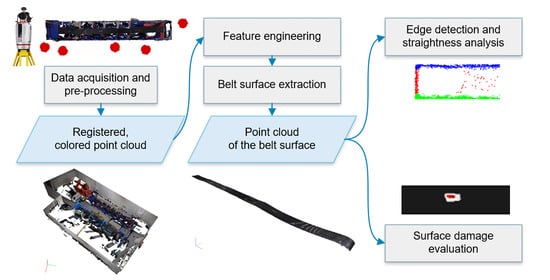
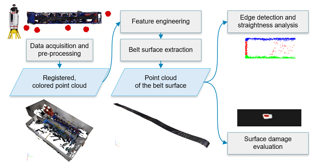
The general outline of proposed workflow of conveyor belt surface inspection based on point cloud data is shown in Figure 1.
Subsequent steps of this workflow are described in detail further in this section and also presented as comprehensive flowcharts in Figure 2, Figure 3, Figure 4 and Figure 5.
2.1. Methodology of Conveyor Belt Geometry Measurement
2.1.1. Data Acquisition
Data acquisition is not the pivotal piece of this study, since multiple measuring devices and methods may be successfully employed to capture the geometrical data in the form of a point cloud. Nevertheless, further processing techniques have specific requirements regarding the input data. Desired input to the processing pipeline should consist of a precise, dense and colored point cloud data with the auxiliary information about reflected laser beam intensity. It may be possible for the described algorithms to work without providing color and intensity data in few cases, although we believe their presence robustifies the process [46,47] through addition of more features to the machine learning classification and easing the operator interpretation of the point cloud during the train data selection. Such data can be collected in various ways. In particular, other than stationary TLS utilized in this study, photogrammetrical and LiDAR measurements carried out with UAV and UGV robots should be considered as suitable solutions.
2.1.2. Point Cloud Data Pre-Processing
Since supervised classification is a vital part of the workflow, distinctive features describing each point and its neighborhood must be calculated first. Feature engineering employed in this paper mostly follows the workflow described in [48] and is presented in Figure 2.
To account for varying point cloud density, geometrical features are computed with respect to the constant k number of closest neighbors for each point. K-d tree of the point cloud is constructed and utilized to compute k-nearest neighbors for every point in the dataset. The number of closest point, determining the size of the neighborhood used in calculations, influences the results of further steps, hence it has to be tuned for specific application. Point cloud resolution, which depends on the instruments and methods used for data collection, will be the major factor affecting size of the neighborhood. Local geometrical features are computed, based on points normal vectors (), eigenvectors and eigenvalues (ordered that ) derived from the point neighborhood [48,49]. Since computing and storing information about k-nearest neighbors for each point in case of processing large point clouds and high values of k may be memory intensive beyond the limits of a standard computer, it is advised that at this step the point cloud is downsampled, e.g., using voxelgrid filter of the chosen spatial resolution. In this study such a filter, implemented in [50], has been employed to downsample the point cloud to the resolution, which allows to carry out the computations on the laptop. Features deemed viable for the classification process and selected for this study are listed in Table 1.
Together with other point cloud scalar fields (RGB colors, intensity), those features will be used as input variables in the supervised classification process. They are then scaled using min-max normalization [51] to the (0, 1) range and the Principal Component Analysis (PCA) is performed on them. Projected features’ usefulness for classification is evaluated using explained variance ratio: the number of components included in the model is chosen in such a way that the cumulative explained variance ratio, attributed by them, amounts to at least 95% of total variance. This contributes both to denoising the data and to simplification of the machine learning model. Thereafter, the pre-processed dataset is ready for the classification process.
2.1.3. Point Cloud Supervised Classification and Segmentation
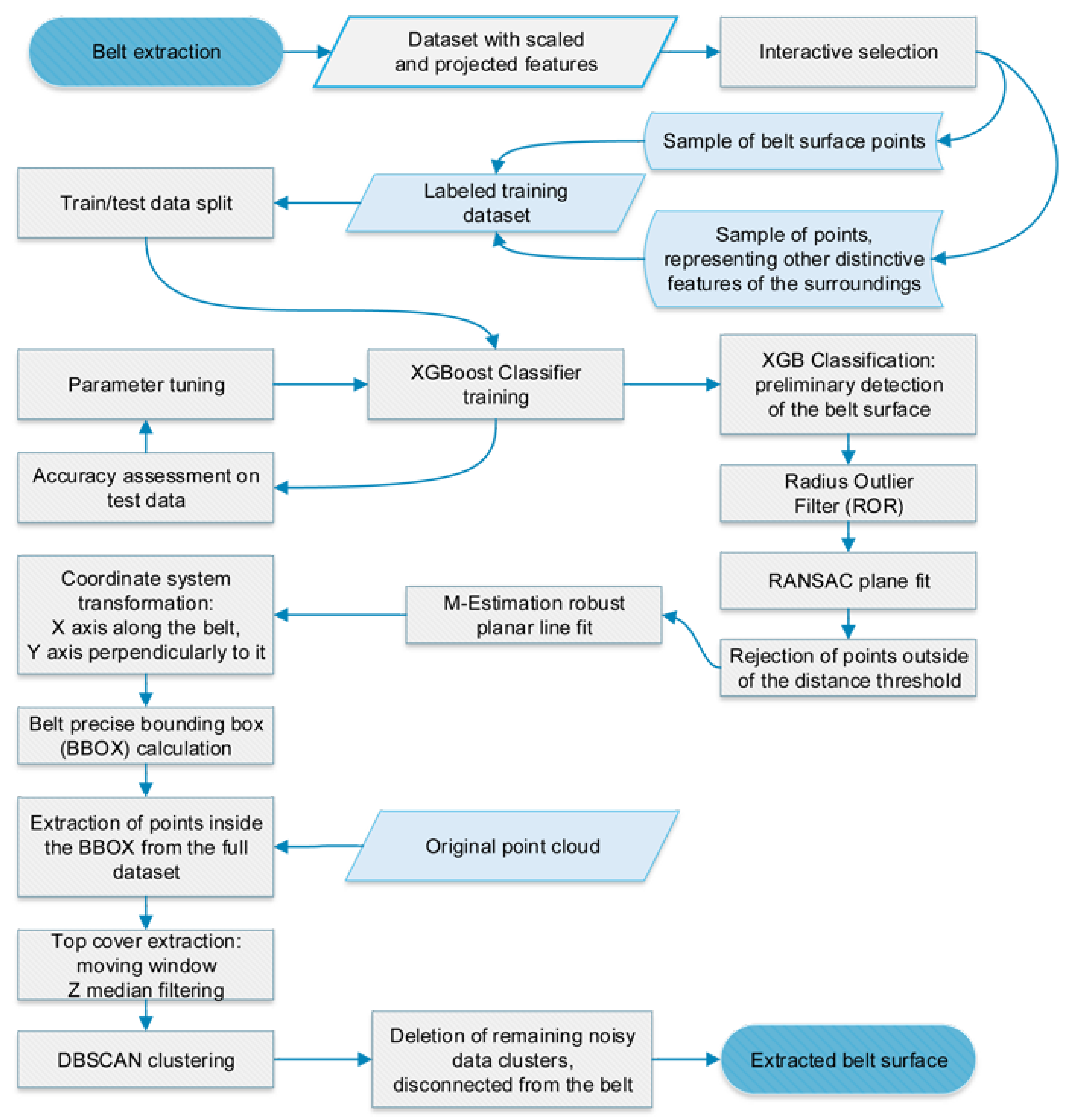
The process of extracting the belt geometry from the point cloud (Figure 3) starts with the supervised classification. Two small training subsets of the colored point cloud are selected interactively by the operator: the former including part of the belt surface and the latter representing distinctive parts of the surroundings such as floor, walls, idlers and other mechanical elements of the belt conveyor. Binary values are then assigned to points accordingly, defining the target variable of the classification, and selected sample is randomly divided into training and test sets in the 4:1 ratio.
Afterwards, training of the eXtreme-Gradient Boosting (XGBoost, [52]) classifier begins. Tree-based model, gbtree, has been employed as a base learner in an ensemble model. Trained model is used to predict labels on the test data and its accuracy is evaluated on metrics such as precision, recall and F score, which are computed as (1), (2) and (3) respectively [51]. Even though the supervised classification is not meant to produce the final differentiation between points representing the belt surface and other elements of the environment, one should assure that the aforementioned metrics are balanced and within reasonable limits. Otherwise, classifier parameters should be iteratively retuned and along with the learning process and its evaluation, they have to be repeated until satisfactory results are achieved.
where:
TP: number of correctly classified points of the belt surface (true positives),
FP: number of points of surroundings incorrectly classified as the belt surface (false positives),
FN: number of points of belt surface incorrectly classified as the surroundings (false negatives).
Radius Outlier Removal (ROR) filter is then used on the belt surface points detected by the XGBoost in order to exclude noise in the form of isolated small groups of points. To further improve quality of belt surface definition, a plane is fit with RANSAC algorithm [53] and points located farther than the threshold are discarded. This step aims to eliminate large groups of false-positive points, which are distant to the belt. The value of the threshold is set to approximately match the height variation of the belt surface.
In the next step, the coordinates are transformed from the former, local coordinate system to the system defined by the major axes of the belt conveyor. Coordinates of preliminarily selected belt points make a basis to create a definition of this reference frame: the x-axis is oriented in the direction of longitudinal dimension of the belt and the y-axis is perpendicular to it. Z-axis remains unchanged. Angle of rotation, required for calculating this transform, is estimated through a line fit into the planar coordinates of abovementioned selection of belt surface points. To minimize influence of possible small number of outliers, line fitting is carried out with Huber robust regressor [54].
At this point, preliminary selection of belt surface points defines the approximation of the real extent of the conveyor belt sufficiently well so that its bounding box can be computed. However, some data may be missing in the interior of the surface due to slightly different properties of splices or damaged areas. To retrieve this information and also enhance spatial resolution of representation of the conveyor belt, original point cloud is loaded again and cropped to the spatial extent defined by the described classification and the nominal width of the belt. This extent, defined by the bounding box, is in a form of a cuboid, hence some data from under the belt (such as parts of idlers), may also get included. To prevent this, a moving window filtering is employed in the next step. The belt is divided into narrow, crosswise strips, and the height median in every strip is calculated. Points lying further from the median height than the presumed accuracy of the data acquisition method are discarded. Lastly, integrity of the belt surface is checked with the Density-Based Spatial Clustering of Applications with Noise (DBSCAN) unsupervised classification algorithm [55]. Only the point cloud coordinates are analyzed. The largest cluster represents the final model of the belt surface. Smaller clusters are ignored, since they represent remaining noise, separated from the belt.
2.2. Belt Geometry Condition Monitoring
2.2.1. Belt Surface Damage Detection
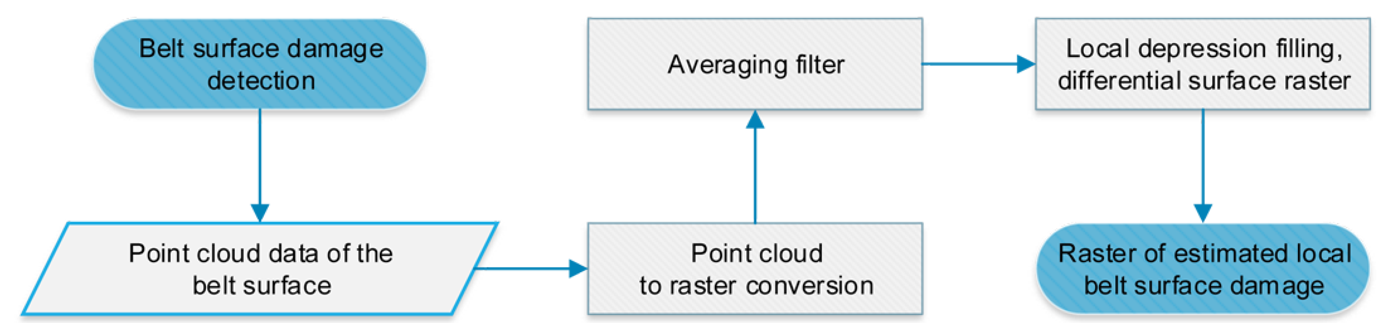
To evaluate condition of the conveyor belt, two main aspects of its representation in the form of a point cloud are analyzed: detection of damaged areas in the belt top cover (Figure 4) and identification of edges’ imperfections (Figure 5). The former examination starts with the conversion of the point cloud into the elevation raster of the belt surface. An averaging filter with a small kernel is then employed to fill missing values in the interior of the raster and reduce the influence of potential outliers. The elevation raster may be interpreted by the operator to manually find damaged areas, although we propose an approximate method for objective damage estimation, based on techniques used in Digital Elevation Model (DEM) analysis. Depression filling algorithm [56,57] is applied to estimate the ideal condition of the belt surface. The difference of this approximation and the raster based on the measurements represents the metric estimate of the top cover damage.
2.2.2. Belt Edges Condition Evaluation
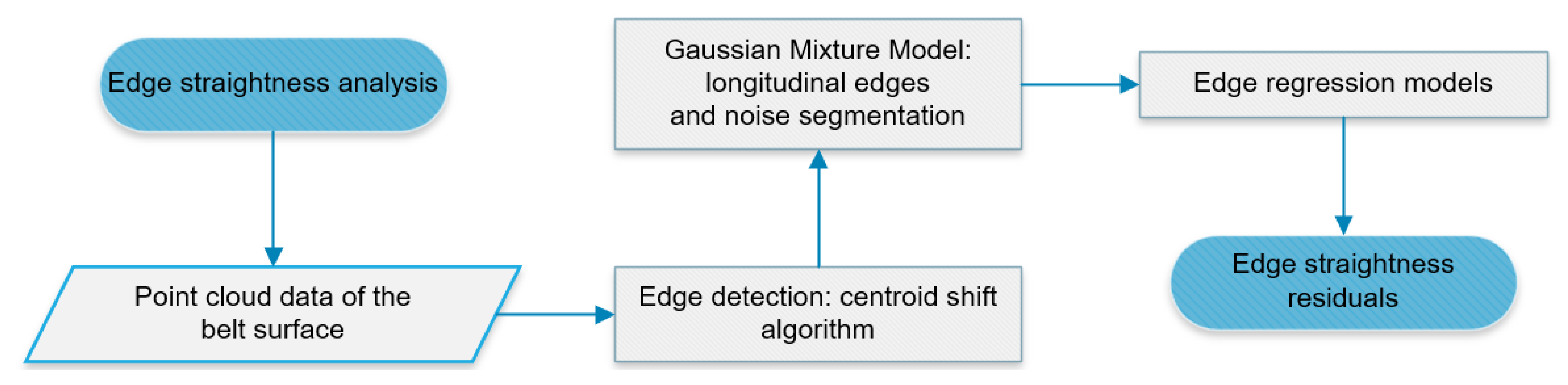
Deformation of the belt edges starts with the algorithm extracting the edges from the conveyor belt point cloud. A centroid shift algorithm, presented in [58] has been applied in our study. One of its advantages is the ability to adjust the width of the detected edges through parameter tuning, which enables retaining edge continuity. Since only the longitudinal edges (top and bottom edges in the belt coordinate system) are the objects of interest, they have to be extracted from all points classified as edges by the abovementioned algorithm. Theoretically, they should be concentrated around two y values, differing by the value of the belt width, with the residuals assumed to be normally distributed. This property is utilized by fitting Gaussian Mixture Model (GMM) unsupervised classifier [59] to the y coordinates of detected edge points. It allows to identify 3 clusters: two main, representing longitudinal belt edges, and the third, containing the noise between them. For evaluating deformations of the edges, residuals from the linear fit are computed for each of them to assess possible deviations from their straight course.
2.3. Test Environment
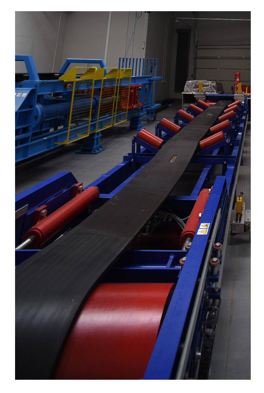
Conveyor belt in the test lab is a steel cord belt with a rubber top cover (Figure 6). It was in overall good condition, since it was used only in the lab environment. Its edges were intact. However, for testing various NDT belt inspection methods, top cover and steel cords in several areas of the belt has been purposely damaged. During our tests 3 main damaged areas were visible: 2 bigger regions, each approximately 25 cm long, 15 cm wide and 1.5 cm deep, and one smaller, which is a 20 cm long, 5 cm wide and 1 cm deep shallow cutout. Moreover, first two areas also had parts of the steel cords extracted, which results in roughly 1 cm of additional cutout depth on a 10 cm long, central part of damaged region (Figure 7). Slow, abrasive wear and non-visible cord breakage are two of the most frequent types of conveyor belt damage, which would be hard to detect with laser scanning. However, Fedorko et al. [60] showed that even when the impact to the belt does not destroy the structure of top cover (no visible cracks), the geometry of the belt is deformed. Furthermore, in hard rock mining, which is our main field of focus, there are cases of serious conveyor belt impact damage, even to the top cover. Damage induced to the belt in the lab, described above, was aimed to simulate such incidents.
For the test measurements, Riegl VZ-400i Figure 8) has been utilized. It is a ToF-based TLS, which can measure up to 500,000 points per second with the angular resolution of 2.5 vertically and 1.8 horizontally. In the device specification [61] the producer states the single point position accuracy to be up to 5 mm. Additionally, photos from the integrated high-resolution panoramic camera (Nikon D810) were taken to add RGB information to the point cloud data in the course of subsequent data processing. In total, five 360 scans with panoramic photos were captured in the lab. Subsequent positions of the laser scanner are shown in the Figure 9. The data was imported into RiSCAN PRO software, where the point clouds were automatically registered and colored. Then, they were exported to a .ply file. Resulting data contains XYZ point coordinates, RGB values describing their color and the value of laser beam intensity. The data has been loaded into Python, where further processing described in Section 2 has been carried out. Several open-source libraries have been utilized: pandas [62], matplotlib [63], scipy [64], scikit-learn [65], PyntCloud [66] and pptk [67].
3. Results
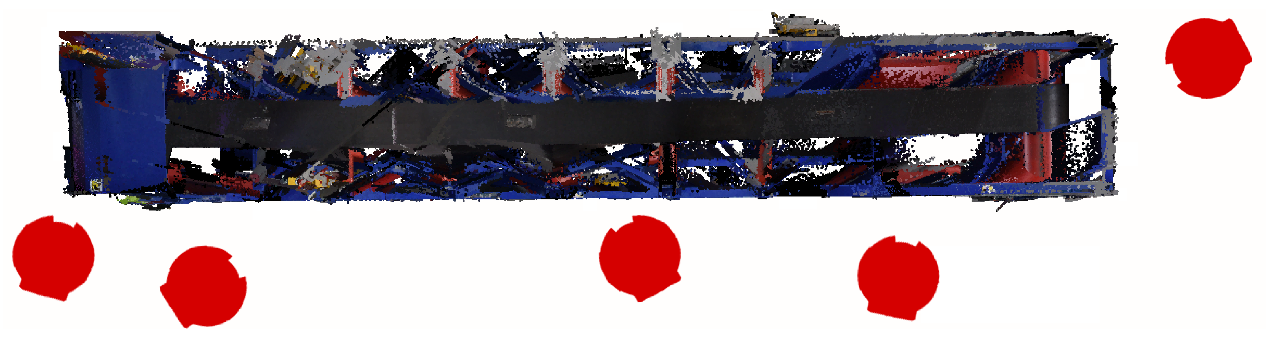
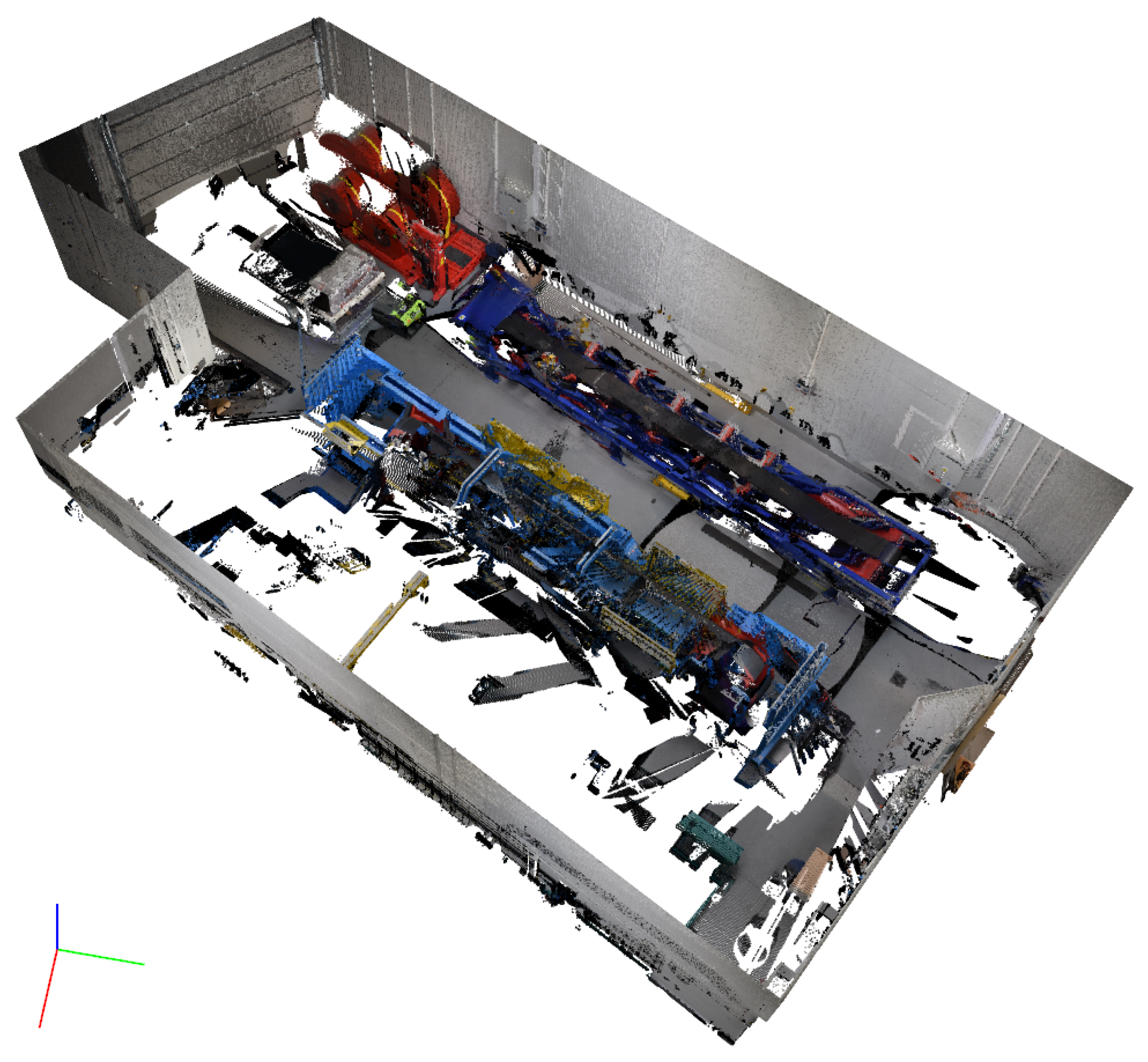
The point cloud data was acquired with the laser scanner from 5 locations, situated in the lab along the belt conveyor (Figure 9). Images were captured with a digital camera, attached to the TLS. The adjustment of the measurements was carried out in the Riegl RiSCAN Pro software in the automatic process. Tie points and planar patches were detected and matched, yielding the final root mean square error (RMSE) of point 3D position of 9.1 mm. Photos were undistorted and joined into panoramic images, which were in turn used for coloring the point cloud data. The resulting dataset consisted of 129,219,560 points and contained information of their 3D coordinates (X, Y and Z in a local coordinate system), laser beam intensity and RGB values. Visualization of the dataset is shown in the Figure 10.
The data was then downsampled with a voxelgrid filter to achieve the resolution of 1.5 cm due to the memory constrains of the processing machine. Filtered dataset consisted of 7,742,055 points. Normal vectors were estimated and geometrical features were calculated based on the neighborhood geometry of each point. The number of neighbors k for a knn algorithm was chosen to be 200. The features were scaled and the PCA was performed. From the initial 14 variables (3 RGB values, intensity and 10 geometrical features), 7 principal components, accounting for 95% of total variance, were extracted. The data was then displayed as in Figure 10 and the operator marked sample areas of the belt surface and other distinctive elements of the surroundings (idlers, wall, floor). Those datasets contained 4527 and 72,425 points respectively. They were randomly split into training and test datasets at a ratio of 4 to 1. Training data was input to the XGB Classifier. The outcomes of its learning were evaluated on selected metrics, which are presented in the Table 2. Although the default parameter values were used in the first iteration of the classifier training, resulting metrics’ values were more than sufficient for the purpose of this first segmenting step of the entire belt extraction process. Over 98% of the belt surface points from the test dataset was correctly detected. In turn, the classification accuracy was deemed to be satisfactory and parameters were not adjusted further. The outcome of this preliminary belt selection can be seen in the Figure 11. In the next step, the main plane of the conveyor belt was estimated using the RANSAC algorithm. The plane containing the most points within the distance of 10 cm was approximated. Points outside of this distance threshold were discarded from further processing (Figure 12).
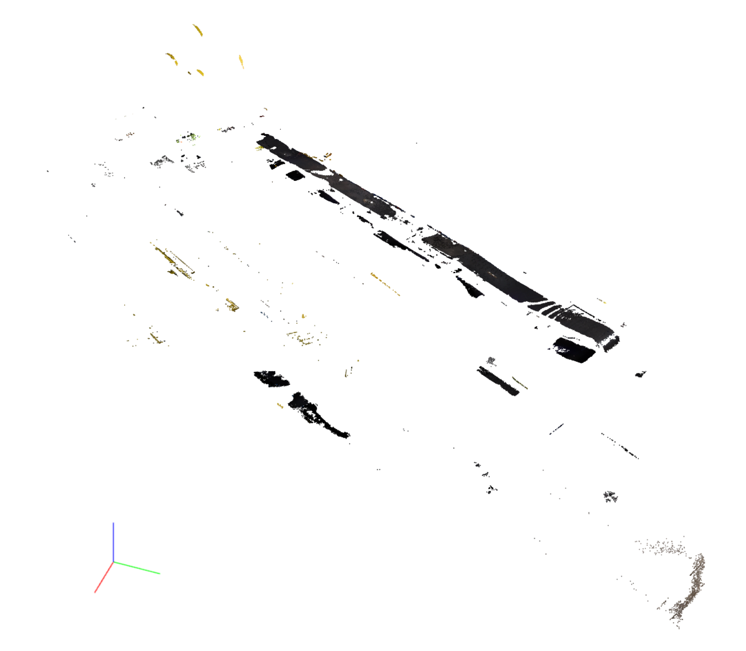
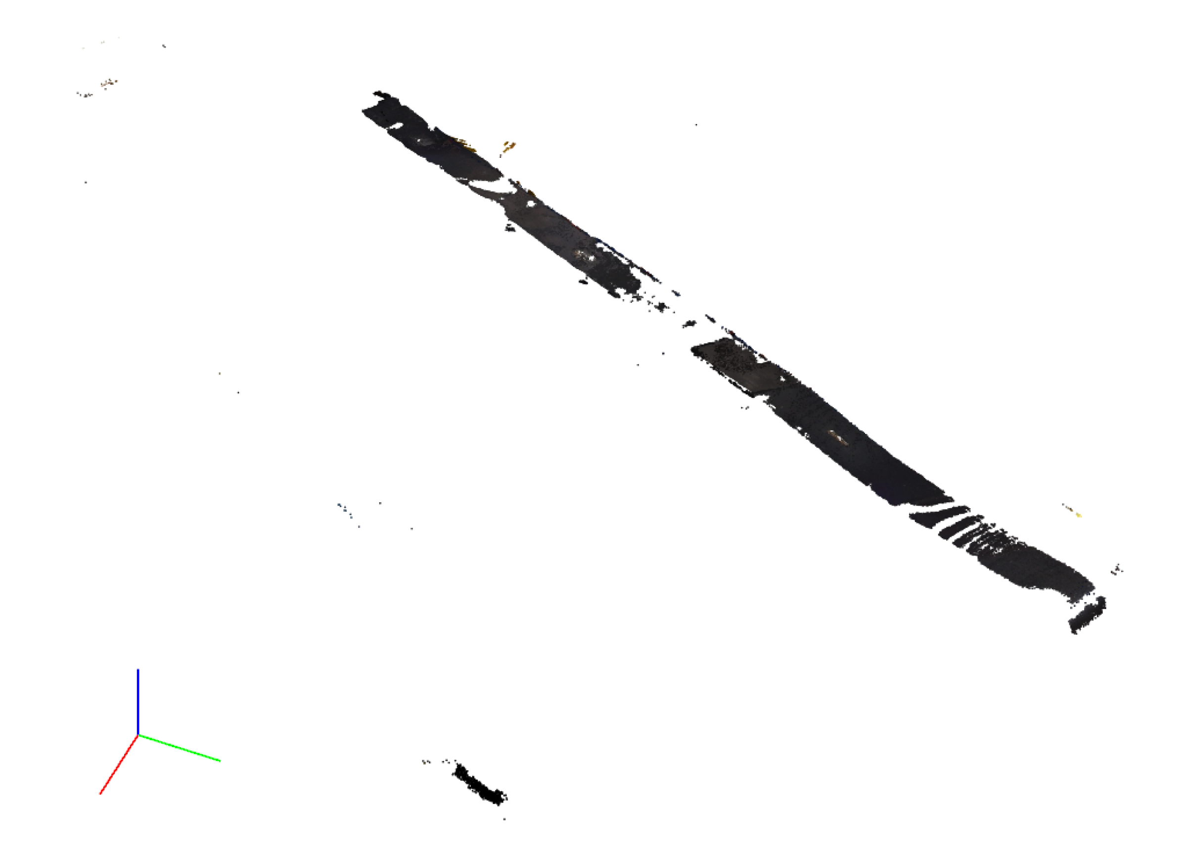
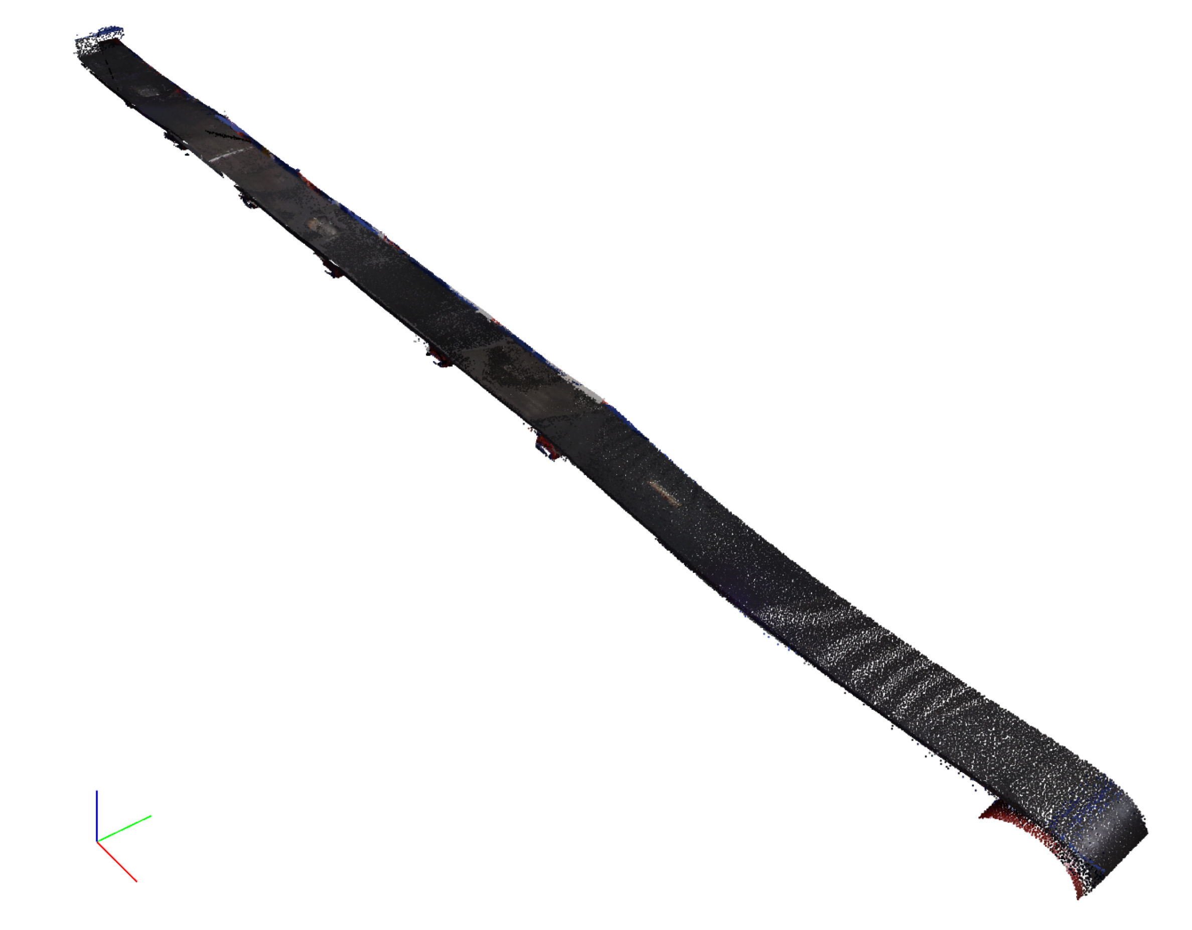
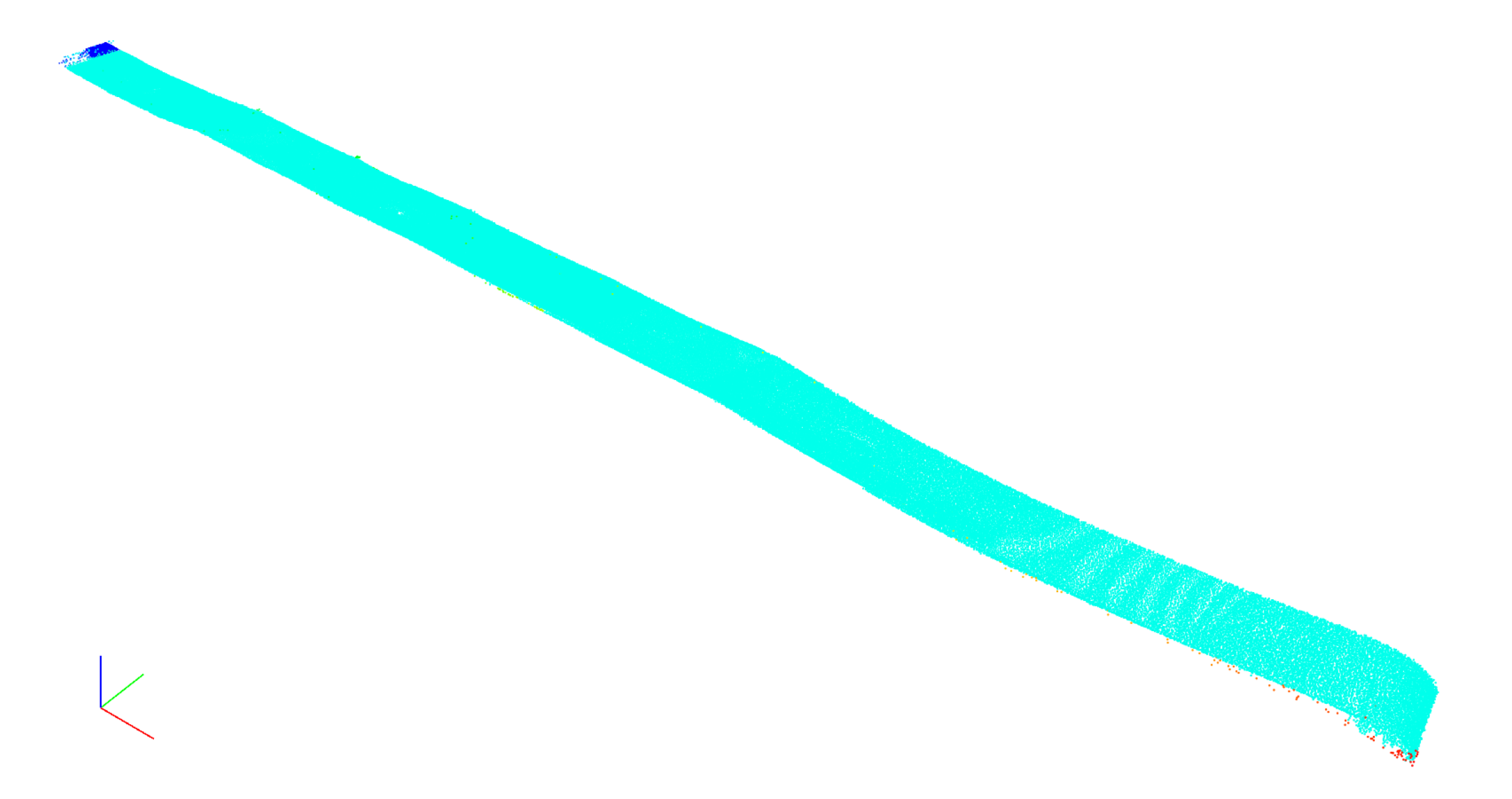
Next, the Huber M-estimator was used for fitting the linear model to the remaining data. This model served as a basis for the coordinate transformation from the local coordinate frame of the TLS to a frame associated with the conveyor belt. The bounding box of point cloud processed in this manner was determined and the initial point cloud was loaded again and cropped to the bounding box limits (Figure 13). The points representing the top cover surface were selected using the moving window filtering procedure and the DBSCAN algorithm was used to discard the remaining points (Figure 14). The final extracted point cloud of the conveyor belt surface is presented in the Figure 15.
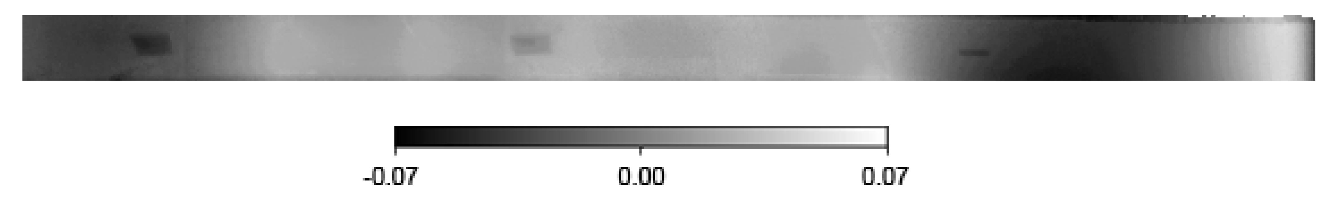
Extracted point cloud of the belt surface was transformed into an elevation raster dataset using binning, i.e., grouping points in a rectangular, planar grid and averaging their Z coordinates in each cell. The resolution of the meshgrid was chosen to be 1 cm. The data was then averaged with a minimal, 3 × 3 kernel to fill any possible voids and eliminate outliers. For presentation purposes, mean elevation was calculated and subtracted from the raster (Figure 16). DEM filling technique was adopted to approximate the belt top cover surface in the ideal condition. Elevation raster from the measurements was subsequently subtracted from this approximation and therefore, local top cover defects, shown in the Figure 17, were estimated. Since the accuracy of single point location, determined by the Riegl VZ-400i TLS measurements, is 5 mm, any damage smaller than 5 mm was deemed to be insignificant and is not indicated in the results. As a result, all of the three test damage areas were correctly detected with the proposed method. However, only a part of the smallest cut has been marked as a damaged belt area. Possible reasons for this have been discussed in the next section.
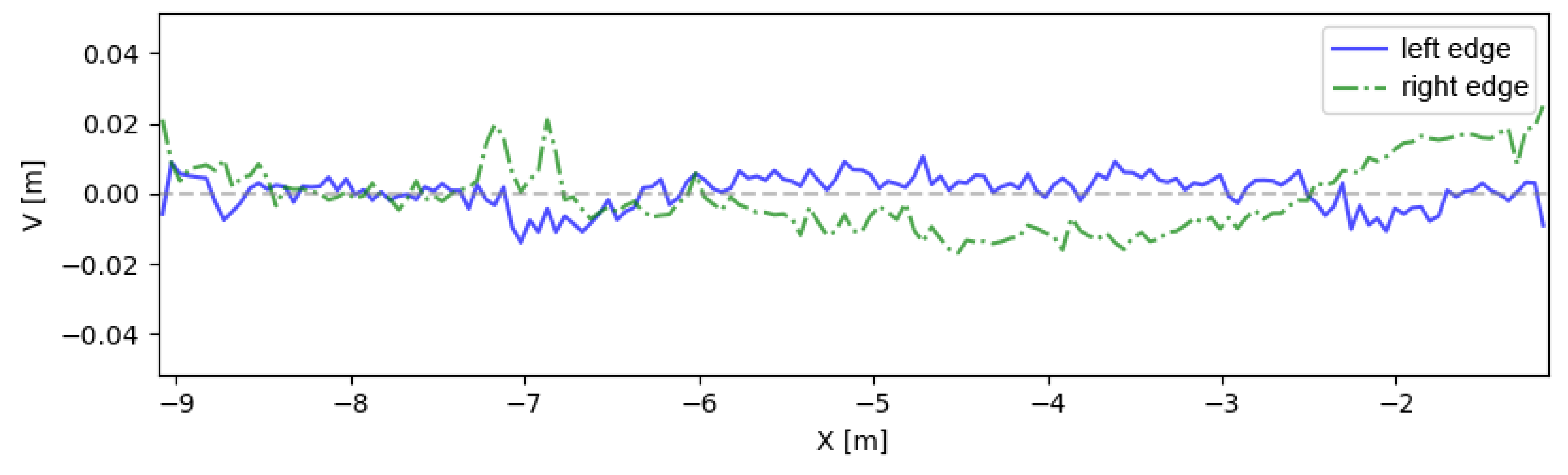
Extracted point cloud data was also used to test the possibility of inspecting the condition of the belt edges. The procedure proposed and implemented in this study consisted of detecting edges with the centroid shift algorithm and segmenting them with GMM classification. In this step, k number of point neighbors for knn search was set at the value of 600 and the method parameter was determined to be 6. Detected and separated edges of the belt, marked in 3 distinctive colors, are depicted in the Figure 18. Finally, points representing longitudinal edges were used to fit two separate linear models. The residuals were calculated, binned and averaged in 5 cm long intervals of the x coordinate for the visualization purposes. The results are presented in the Figure 19. Since no damage was induced to the edges of the conveyor belt in the test lab and considering the accuracy of TLS measurements and further data processing, maximum achieved deviations from the straight line, reaching 2 cm, should be considered the precision of the proposed inspection method. Moreover, as in the case of investigating surface damage on the elevation raster, edges’ condition can be additionally verified through manual examination of extracted and classified point cloud, shown in the Figure 18.
4. Discussion
We believe that our approach utilising rapid construction of a detailed geometric model of the belt surface method is an advancement and enhancement of presently used techniques in the mining industry for conveyor belt surface inspection and evaluation, such as visual methods, magnetic methods with signal processing, applicable for steel cord belts [9,10,11] or detection of belt’s tear with ultrasonic sensors [12]. The proposed method of semi-automatic point cloud data processing obtained with TLS for inspection of conveyor belts provides accuracy appropriate for identification of damage induced to belt’s surface during haulage of material in underground and open-cast mine environment. The procedure has been successfully tested in laboratory conditions. The test proved that our approach is suitable for detecting damaged areas of the belt surface, which were at least 1 cm deep. The biggest factor, limiting the accuracy of the proposed method during the test measurements, was the accuracy of the ToF-based TLS. As stated in the Section 1, TLS using phase-shift estimation usually provide better accuracy of point location than ToF-based TLS. Therefore, it may be possible to further enhance the accuracy and sensitivity of our method through using such a device.
Another issue, indicated previously in the Section 3, is that for the narrowest of the damaged areas, only a part of it was correctly detected. This could be the consequence of carrying out the TLS measurements at an acute angle, from the side of the belt conveyor. Data captured from higher elevation, e.g., from a sensor mounted on a drone flying over the conveyor, might be better suited for detecting such damage. This should minimize any occlusions of damaged areas and as a result, prevent underestimations of surface damage. The limitation of the methodology is also that it requires the stationarity of the belt, while the sensor capturing the data is the one changing position. This may not always be the disadvantage, although it is contrary to the majority of the other methods for conveyor belt condition evaluation, where the sensor is usually mounted in a fixed position and the belt is moving underneath or above it. However, during the mining operation cycle, there are periods when the conveyor is not operating and not carrying any bulk material. Currently, during this temporary halt, visual inspection is often manually being performed by the maintenance staff. This is also when measurements with our method can be performed on the stationary belt without disruption to the mining process.
The presented methodology is designed to provide only the information about the surface and the edges of the conveyor belt. Even though this components of conveyors are the ones of the most susceptible to getting damaged, other elements of the belt conveyor system, such as internal parts of the belt (e.g., steel cords), bearings or idlers, must be monitored with other methods, described in Section 1. However, our methodology can be combined with those other NDT techniques. Known NDT methods studied and used for steel cord belts monitoring are based on electromagnetic measurements and include: inductive, reluctance, induced voltage, X-ray and ultrasonic techniques. Whereas, in case of fabric belts capacitive, ultrasonic and X-ray methods have been applied [24]. Fusing those methods with our approach would provide more comprehensive information for better understanding of conveyor belt characteristics and improved design and construction of conveyor belt systems. Thus, it could lead to reduction of system’s maintenance costs, shorter downtime and increased system’s life.
Special attention must be paid to the conditions of the target application site, i.e., an underground mine. Although we conducted our tests in a controlled lab environment, influence of selected environmental factors, present in a mine, should be considered. The most dangerous factor seems to be dust, which could potentially both harm the sensor and introduce additional noise in collected data. To mitigate the former problem, a device with appropriate Ingress Protection (IP) Rating should be used (sensor employed in this study complies to the IP64 norm) or alternatively, a High Efficiency Particulate Air (HEPA) filter may be used in ventilation system of a TLS. The latter issue is for the most part alleviated through using outlier filters during the point cloud processing, mentioned in Section 2. They should prevent the influence of incorrect points, caused by the laser beam hitting dust particles in the air, on the processing results. It should be noted, that in such environment the main source of dusting is the moving conveyor itself. Thus, its stationarity greatly reduces dustiness during the measurements. Nonetheless, presence of heavy dust would lead to slight deterioration of sensor accuracy and as a result, lowering the damage size, which we would be able to detect.
Another factor, important for any visual inspection method, is lightning. In underground mine corridors with conveyors, it is usually poor and uneven. This is problematic for many visual 3D modelling methods, e.g., based on photogrammetry. For laser scanning, this is not an issue, since scene illumination is not necessary for reconstructing its geometry. Simultaneous image acquisition may be carried out, but because it provides only a supplementary information about points’ colors, uneven exposure or weak lightning should not significantly affect proposed method.
5. Conclusions
In the paper a novel approach for belt geometry identification and its interpretation in the context of conveyor belt condition evaluation is proposed. We have used laser scanning to acquire point cloud data and create the geometrical model of the belt conveyor in the laboratory conditions and with simulated damages. Thanks to developed algorithms, we were able to extract data that describe shape of the belt and detect its surface irregularities and evaluate the roughness of the edges. Such information is important for maintenance staff and until now, it has been acquired by visual inspection only. Objective and metric methods of belt condition evaluation, such as the one presented in this paper, are more reliable than human interpretation. Moreover, it can be compared with subsequent measurements in order to evaluate the progress in damage development. The created 3D model of the conveyor belt can be stored in case of the need to carry out additional measurements and investigation of the conveyor belt condition in the future. Further research of presented methodology will be focused on its application in the harsh environment of a real underground mine and additional possibilities of input data sources, such as drone imagery or mobile laser scanning, for data acquisition.
Author Contributions
Conceptualization: P.T., R.Z.; Methodology: P.T.; Investigation: P.T.; Software: P.T.; Formal analysis: P.T.; Visualization: P.T.; Resources: R.B.; Writing—Original Draft: P.T. R.Z.; Writing—Review & Editing: J.B., R.Z., R.B.; Supervision: R.Z., J.B.; Funding acquisition: R.Z. All authors have read and agreed to the published version of the manuscript.
Funding
This activity has received funding from European Institute of Innovation and Technology (EIT), a body of the European Union, under the Horizon 2020, the EU Framework Programme for Research and Innovation. This work is supported by EIT RawMaterials GmbH under Framework Partnership Agreement No. 19018 (AMICOS. Autonomous Monitoring and Control System for Mining Plants).
Conflicts of Interest
The authors declare no conflict of interest. The funders had no role in the design of the study; in the collection, analyses, or interpretation of data; in the writing of the manuscript, or in the decision to publish the results.
References
- Wodecki, J.; Zdunek, R.; Wyłomańska, A.; Zimroz, R. Local fault detection of rolling element bearing components by spectrogram clustering with Semi-Binary NMF. Diagnostyka 2017, 18, 3–8. [Google Scholar]
- Wodecki, J.; Michalak, A.; Zimroz, R.; Wyłomańska, A. Separation of multiple local-damage-related components from vibration data using Nonnegative Matrix Factorization and multichannel data fusion. Mech. Syst. Signal Process. 2020, 145. [Google Scholar] [CrossRef]
- Obuchowski, J.; Wylomańska, A.; Zimroz, R. Recent developments in vibration based diagnostics of gear and bearings used in belt conveyors. Appl. Mech. Mater. 2014, 683, 171–176. [Google Scholar] [CrossRef]
- Gładysiewicz, L.; Król, R.; Kisielewski, W. Measurements of loads on belt conveyor idlers operated in real conditions. Meas. J. Int. Meas. Confed. 2019, 134, 336–344. [Google Scholar] [CrossRef]
- Król, R.; Kisielewski, W.; Kaszuba, D.; Gładysiewicz, L. Testing belt conveyor resistance to motion in underground mine conditions. Int. J. Min. Reclam. Environ. 2017, 31, 78–90. [Google Scholar] [CrossRef]
- Molnar, V.; Fedorko, G.; Honus, S.; Andrejiova, M.; Grincova, A.; Michalik, P.; Palenčár, J. Research in Placement of Measuring Sensors on Hexagonal Idler Housing with regard to Requirements of Pipe Conveyor Failure Analysis. Eng. Fail. Anal. 2020, 116, 104703. [Google Scholar] [CrossRef]
- Molnár, V.; Fedorko, G.; Homolka, L.; Michalik, P.; Tučková, Z. Utilisation of measurements to predict the relationship between contact forces on the pipe conveyor idler rollers and the tension force of the conveyor belt. Measurement 2019, 136, 735–744. [Google Scholar] [CrossRef]
- Kozłowski, T.; Wodecki, J.; Zimroz, R.; Błażej, R.; Hardygóra, M. A Diagnostics of Conveyor Belt Splices. Appl. Sci. 2020, 10, 6259. [Google Scholar] [CrossRef]
- Blazej, R.; Jurdziak, L.; Zimroz, R. Novel approaches for processing of multi-channels NDT signals for damage detection in conveyor belts with steel cords. Key Eng. Mater. 2013, 569–570, 978–985. [Google Scholar] [CrossRef]
- Kozłowski, T.; Błażej, R.; Jurdziak, L.; Kirjanów-Błażej, A. Magnetic methods in monitoring changes of the technical condition of splices in steel cord conveyor belts. Eng. Fail. Anal. 2019, 104, 462–470. [Google Scholar] [CrossRef]
- Błażej, R.; Jurdziak, L.; Kozłowski, T.; Kirjanów, A. The use of magnetic sensors in monitoring the condition of the core in steel cord conveyor belts—Tests of the measuring probe and the design of the DiagBelt system. Meas. J. Int. Meas. Confed. 2018, 123, 48–53. [Google Scholar] [CrossRef]
- Błazej, R.; Jurdziak, L.; Kirjanów, A.; Kozłowski, T. A device for measuring conveyor belt thickness and for evaluating the changes in belt transverse and longitudinal profile. Diagnostyka 2017, 18, 97–102. [Google Scholar]
- Valis, D.; Mazurkiewicz, D.; Forbelska, M. Modelling of a transport belt degradation using state space model. In Proceedings of the 2017 IEEE International Conference on Industrial Engineering and Engineering Management (IEEM), Singapore, 10–13 December 2017; pp. 949–953. [Google Scholar]
- Doroszuk, B.; Król, R. Analysis of conveyor belt wear caused by material acceleration in transfer stations. Min. Sci. 2019, 26, 189–201. [Google Scholar] [CrossRef]
- Bajda, M.; Błażej, R.; Hardygóra, M. Optimizing splice geometry in multiply conveyor belts| with respect to stress in adhesive bonds. Min. Sci. 2018, 25, 195–206. [Google Scholar] [CrossRef]
- Zhang, S.; Xia, X. Optimal control of operation efficiency of belt conveyor systems. Appl. Energy 2010, 87, 1929–1937. [Google Scholar] [CrossRef]
- Zhang, X.; Fan, T. The Research of Distribute Temperature Monitoring System Early Warning Fire in Coal Belt Conveyor. Adv. Mater. Res. 2012, 548, 890–892. [Google Scholar] [CrossRef]
- Sawicki, M.; Zimroz, R.; Wyłomańska, A.; Obuchowski, J.; Stefaniak, P.; Żak, G. An Automatic Procedure for Multidimensional Temperature Signal Analysis of a SCADA System with Application to Belt Conveyor Components. Procedia Earth Planet. Sci. 2015, 15, 781–790. [Google Scholar] [CrossRef] [Green Version]
- Michalik, P.; Zajac, J. Use of thermovision for monitoring temperature conveyor belt of pipe conveyor. Appl. Mech. Mater. 2014, 683, 238–242. [Google Scholar] [CrossRef]
- Liu, X.; Pang, Y.; Lodewijks, G.; He, D. Experimental research on condition monitoring of belt conveyor idlers. Measurement 2018, 127, 277–282. [Google Scholar] [CrossRef]
- Zimroz, R.; Hutter, M.; Mistry, M.; Stefaniak, P.; Walas, K.; Wodecki, J. Why Should Inspection Robots be used in Deep Underground Mines? In Proceedings of the 27th International Symposium on Mine Planning and Equipment Selection—MPES 2018; Widzyk-Capehart, E., Hekmat, A., Singhal, R., Eds.; Springer International Publishing: Cham, Switzerland, 2019; pp. 497–507. [Google Scholar]
- Carvalho, R.; Nascimento, R.; D’Angelo, T.; Delabrida, S.; Bianchi, A.G.C.; Oliveira, R.A.; Azpúrua, H.; Uzeda Garcia, L.G. A UAV-Based Framework for Semi-Automated Thermographic Inspection of Belt Conveyors in the Mining Industry. Sensors 2020, 20, 2243. [Google Scholar] [CrossRef] [Green Version]
- Szrek, J.; Wodecki, J.; Błażej, R.; Zimroz, R. An Inspection Robot for Belt Conveyor Maintenance in Underground Mine—Infrared Thermography for Overheated Idlers Detection. Appl. Sci. 2020, 10, 4984. [Google Scholar] [CrossRef]
- Zimroz, R.; Hardygóra, M.; Blazej, R. Maintenance of Belt Conveyor Systems in Poland—An Overview. In Proceedings of the 12th International Symposium Continuous Surface Mining—Aachen 2014; Niemann-Delius, C., Ed.; Springer International Publishing: Cham, Switzerland, 2015; pp. 21–30. [Google Scholar]
- Blazej, R.; Zimroz, R.; Jurdziak, L.; Hardygora, M.; Kawalec, W. Conveyor belt condition evaluation via non-destructive testing techniques. In Mine Planning And Equipment Selection; Springer: Cham, Switzerland, 2014; pp. 1119–1126. [Google Scholar]
- Chauve, A.; Mallet, C.; Bretar, F.; Durrieu, S.; Deseilligny, M.P.; Puech, W. Processing full-waveform lidar data: Modelling raw signals. Int. Arch. Photogramm. Remote Sens. Spat. Inf. Sci. 2006, 36.3/W52, 102–107. [Google Scholar]
- Fregonese, L.; Barbieri, G.; Biolzi, L.; Bocciarelli, M.; Frigeri, A.; Taffurelli, L. Surveying and monitoring for vulnerability assessment of an ancient building. Sensors 2013, 13, 9747–9773. [Google Scholar] [CrossRef] [PubMed]
- Alba, M.; Fregonese, L.; Prandi, F.; Scaioni, M.; Valgoi, P. Structural monitoring of a large dam by terrestrial laser scanning. Int. Arch. Photogramm. Remote Sens. Spat. Inf. Sci. 2006, 36, 6. [Google Scholar]
- Muszynski, Z.; Milczarek, W. Application of terrestrial laser scanning to study the geometry of slender objects. IOP Conf. Ser. Earth Environ. Sci. 2017, 95, 42–69. [Google Scholar] [CrossRef] [Green Version]
- Wehr, A.; Lohr, U. Airborne laser scanning—An introduction and overview. ISPRS J. Photogramm. Remote Sens. 1999, 54, 68–82. [Google Scholar] [CrossRef]
- Bellian, J.A.; Kerans, C.; Jennette, D.C. Digital outcrop models: Applications of terrestrial scanning lidar technology in stratigraphic modeling. J. Sediment. Res. 2005, 75, 166–176. [Google Scholar] [CrossRef] [Green Version]
- Fernández-Lozano, J.; Gutiérrez-Alonso, G.; Fernández-Morán, M.Á. Using airborne LiDAR sensing technology and aerial orthoimages to unravel roman water supply systems and gold works in NW Spain (Eria valley, León). J. Archaeol. Sci. 2015, 53, 356–373. [Google Scholar] [CrossRef]
- Dubayah, R.O.; Drake, J.B. Lidar remote sensing for forestry. J. For. 2000, 98, 44–46. [Google Scholar]
- Rosell, J.; Sanz, R. A review of methods and applications of the geometric characterization of tree crops in agricultural activities. Comput. Electron. Agric. 2012, 81, 124–141. [Google Scholar] [CrossRef] [Green Version]
- Weitkamp, C. (Ed.) Lidar: Range-Resolved Optical Remote Sensing of the Atmosphere; Springer: New York, NY, USA, 2006. [Google Scholar]
- Cheng, Y.; Wang, G.Y. Mobile robot navigation based on lidar. In Proceedings of the 2018 Chinese Control And Decision Conference (CCDC), Shenyang, China, 9–11 June 2018; pp. 1243–1246. [Google Scholar]
- Biber, P.; Andreasson, H.; Duckett, T.; Schilling, A. 3D modeling of indoor environments by a mobile robot with a laser scanner and panoramic camera. In Proceedings of the 2004 IEEE/RSJ International Conference on Intelligent Robots and Systems (IROS) (IEEE Cat. No. 04CH37566), Sendai, Japan, 28 September–2 October 2004; Volume 4, pp. 3430–3435. [Google Scholar]
- Zhang, W.; Yang, D. Lidar-Based Fast 3D Stockpile Modeling. In Proceedings of the 2019 International Conference on Intelligent Computing, Automation and Systems (ICICAS), Chongqing, China, 6–8 December 2019; pp. 703–707. [Google Scholar]
- Duff, E. Automated volume estimation of haul-truck loads. In Proceedings of the Australian Conference on Robotics and Automation, Melbourne, Australia, 30 August–1 September 2000; CSIRO: Melbourne, Australia, 2000; pp. 179–184. [Google Scholar]
- Kukutsch, R.; Konicek, P.; Waclawik, P.; Ptáček, J.; Kajzar, V. Possibility of convergence measurement of gates in coal mining using terrestrial 3D laser scanner. J. Sustain. Min. 2015, 14. [Google Scholar] [CrossRef] [Green Version]
- Kajzar, V. Verifying the possibilities of using a 3D laser scanner in the mining underground. Acta Geodyn. Geomater. 2015, 51–58. [Google Scholar] [CrossRef] [Green Version]
- Zeng, F.; Wu, Q.; Chu, X.; Yue, Z. Measurement of bulk material flow based on laser scanning technology for the energy efficiency improvement of belt conveyors. Measurement 2015, 75, 230–243. [Google Scholar] [CrossRef]
- Fengyun, G.; Hongquan, X. Status and development trend of 3D laser scanning technology in the mining field. In Proceedings of the 2013 the International Conference on Remote Sensing, Environment and Transportation Engineering (RSETE 2013), Nanjing, China, 26–28 July 2013; Atlantis Press: Paris, France, 2013; pp. 405–408. [Google Scholar] [CrossRef]
- Neumann, T.; Ferrein, A.; Kallweit, S.; Scholl, I. Towards a mobile mapping robot for underground mines. In Proceedings of the 2014 PRASA, RobMech and AfLaI Int. Joint Symposium, Cape Town, South Africa, 27–28 November 2014. [Google Scholar]
- Grilli, E.; Menna, F.; Remondino, F. A review of point clouds segmentation and classification algorithms. Int. Arch. Photogramm. Remote Sens. Spat. Inf. Sci. 2017, 42, 339. [Google Scholar] [CrossRef] [Green Version]
- Strom, J.; Richardson, A.; Olson, E. Graph-based segmentation for colored 3D laser point clouds. In 2010 IEEE/RSJ International Conference on Intelligent Robots and Systems; IEEE: Piscataway, NJ, USA, 2010; pp. 2131–2136. [Google Scholar]
- Reymann, C.; Lacroix, S. Improving LiDAR point cloud classification using intensities and multiple echoes. In Proceedings of the 2015 IEEE/RSJ International Conference on Intelligent Robots and Systems (IROS), Hamburg, Germany, 28 September–3 October 2015; pp. 5122–5128. [Google Scholar]
- Weinmann, M.; Jutzi, B.; Hinz, S.; Mallet, C. Semantic point cloud interpretation based on optimal neighborhoods, relevant features and efficient classifiers. ISPRS J. Photogramm. Remote Sens. 2015, 105, 286–304. [Google Scholar] [CrossRef]
- Weinmann, M.; Weinmann, M.; Mallet, C.; Brédif, M. A classification-segmentation framework for the detection of individual trees in dense MMS point cloud data acquired in urban areas. Remote Sens. 2017, 9, 277. [Google Scholar] [CrossRef] [Green Version]
- Zhou, Q.Y.; Park, J.; Koltun, V. Open3D: A Modern Library for 3D Data Processing. arXiv 2018, arXiv:1801.09847. [Google Scholar]
- Géron, A. Hands-on Machine Learning with Scikit-Learn, Keras, and TensorFlow: Concepts, Tools, and Techniques to Build Intelligent Systems; O’Reilly Media: Sebastopol, CA, USA, 2019. [Google Scholar]
- Chen, T.; Guestrin, C. XGBoost: A Scalable Tree Boosting System. In Proceedings of the 22nd ACM SIGKDD International Conference on Knowledge Discovery and Data Mining (KDD ’16), San Francisco, CA, USA, 13–17 August 2016; ACM: New York, NY, USA, 2016; pp. 785–794. [Google Scholar] [CrossRef] [Green Version]
- Schnabel, R.; Wahl, R.; Klein, R. Efficient RANSAC for point-cloud shape detection. Comput. Graph. Forum 2007, 26, 214–226. [Google Scholar] [CrossRef]
- Huber, P.J. Robust Statistics; Wiley: Hoboken, NJ, USA, 2004; Volume 523. [Google Scholar]
- Schubert, E.; Sander, J.; Ester, M.; Kriegel, H.P.; Xu, X. DBSCAN revisited, revisited: Why and how you should (still) use DBSCAN. ACM Trans. Database Syst. (TODS) 2017, 42, 1–21. [Google Scholar] [CrossRef]
- Barnes, R. RichDEM: Terrain Analysis Software. 2016. Available online: http://github.com/r-barnes/richdem (accessed on 31 October 2020).
- Zhou, G.; Sun, Z.; Fu, S. An efficient variant of the priority-flood algorithm for filling depressions in raster digital elevation models. Comput. Geosci. 2016, 90, 87–96. [Google Scholar] [CrossRef]
- Ahmed, S.M.; Tan, Y.Z.; Chew, C.M.; Al Mamun, A.; Wong, F.S. Edge and corner detection for unorganized 3D point clouds with application to robotic welding. In Proceedings of the 2018 IEEE/RSJ International Conference on Intelligent Robots and Systems (IROS), Madrid, Spain, 1–5 October 2018; pp. 7350–7355. [Google Scholar]
- Reynolds, D.A. Gaussian Mixture Models. Encycl. Biom. 2009, 741. [Google Scholar]
- Fedorko, G.; Molnar, V.; Marasova, D.; Grincova, A.; Dovica, M.; Zivcak, J.; Toth, T.; Husakova, N. Failure analysis of belt conveyor damage caused by the falling material. Part II: Application of computer metrotomography. Eng. Fail. Anal. 2013, 34, 431–442. [Google Scholar] [CrossRef]
- RIEGL VZ-400i Datasheet. 2019. Available online: http://www.riegl.com/uploads/tx_pxpriegldownloads/RIEGL_VZ-400i_Datasheet_2020-10-06.pdf (accessed on 31 October 2020).
- McKinney, W. Data Structures for Statistical Computing in Python. In Proceedings of the 9th Python in Science Conference, Austin, TX, USA, 28–30 June 2010; pp. 51–56. [Google Scholar]
- Hunter, J.D. Matplotlib: A 2D graphics environment. Comput. Sci. Eng. 2007, 9, 90–95. [Google Scholar] [CrossRef]
- Virtanen, P.; Gommers, R.; Oliphant, T.E.; Haberland, M.; Reddy, T.; Cournapeau, D.; Burovski, E.; Peterson, P.; Weckesser, W.; Bright, J.; et al. SciPy 1.0: Fundamental Algorithms for Scientific Computing in Python. Nat. Methods 2020. [Google Scholar] [CrossRef] [PubMed] [Green Version]
- Pedregosa, F.; Varoquaux, G.; Gramfort, A.; Michel, V.; Thirion, B.; Grisel, O.; Blondel, M.; Prettenhofer, P.; Weiss, R.; Dubourg, V.; et al. Scikit-learn: Machine Learning in Python. J. Mach. Learn. Res. 2011, 12, 2825–2830. [Google Scholar]
- de la Iglesia Castro, D. PyntCloud. 2019. Available online: https://github.com/daavoo/pyntcloud (accessed on 31 October 2020).
- pptk—Point Processing Toolkit. 2018. Available online: https://github.com/heremaps/pptk (accessed on 31 October 2020).
Figure 1.
Data processing overview.
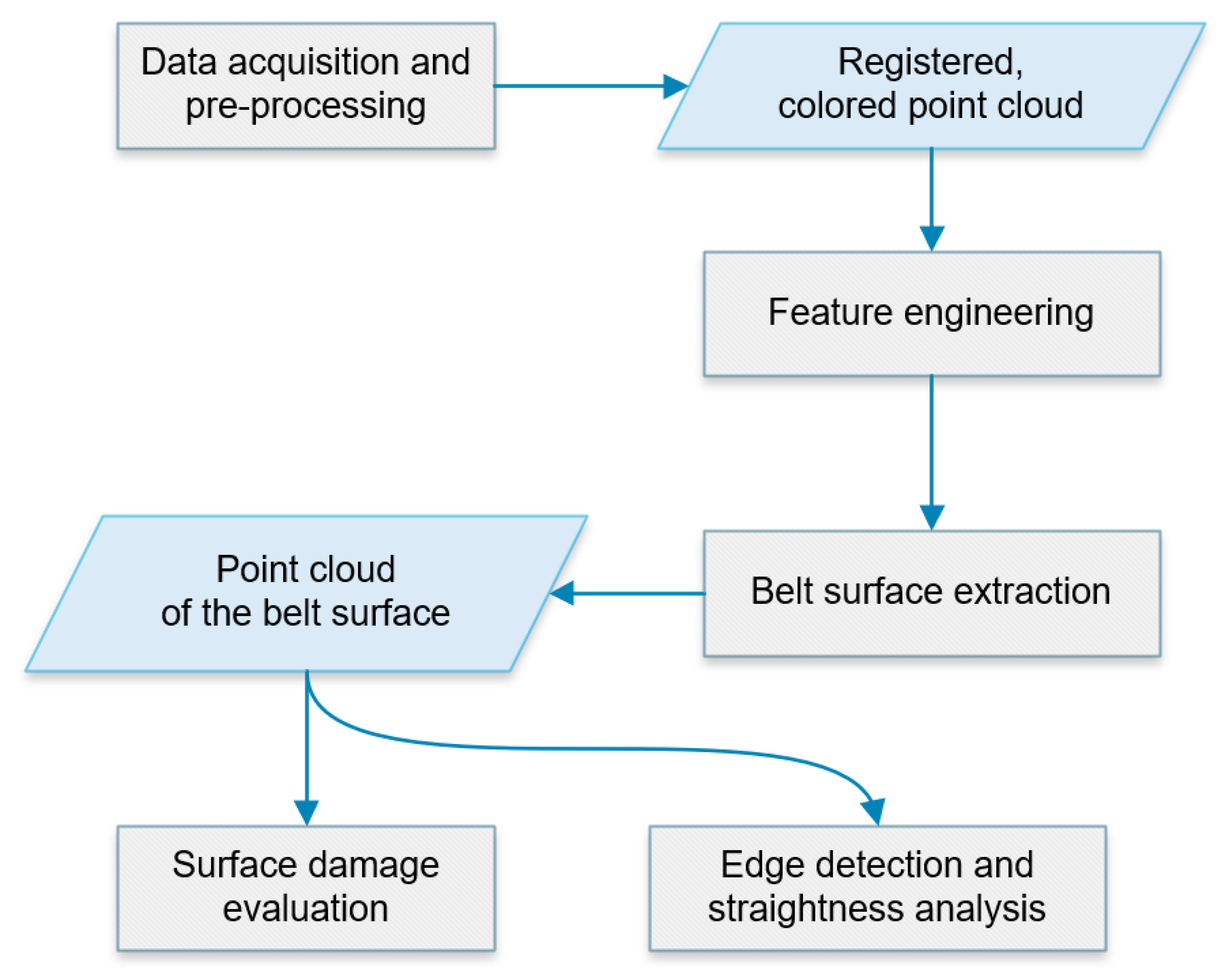
Figure 2.
Feature engineering for classification.
Figure 3.
Workflow of belt extraction procedure.

Figure 4.
Workflow of belt surface local irregularities identification.

Figure 5.
Workflow of belt edge detection and their straightness evaluation.

Figure 6.
Belt conveyor test rig in GEO3EM Research Center at WUST.

Figure 7.
Example of the damage induced to the conveyor belt.
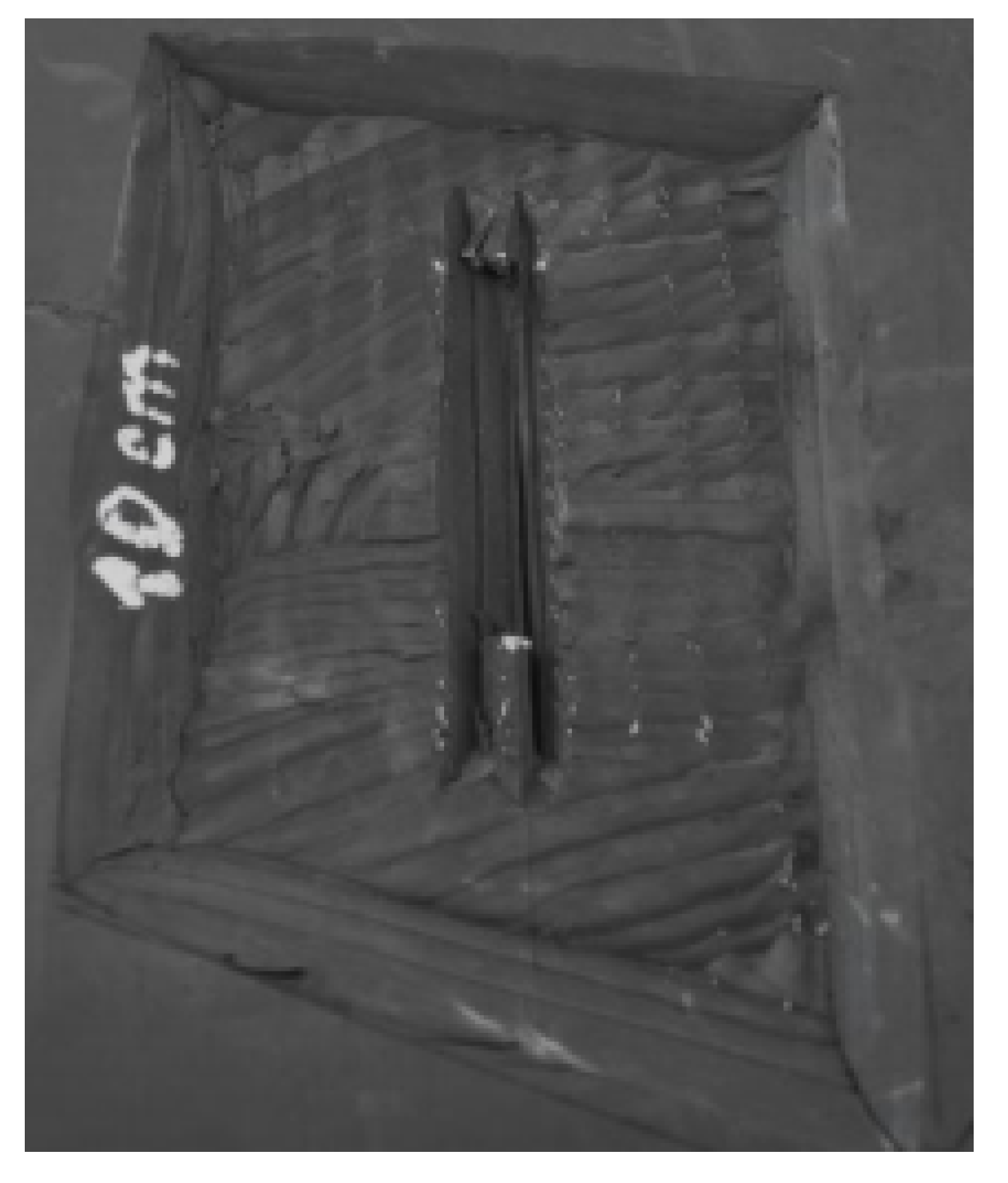
Figure 8.
Riegl VZ-400i TLS [61].
Figure 8.
Riegl VZ-400i TLS [61].
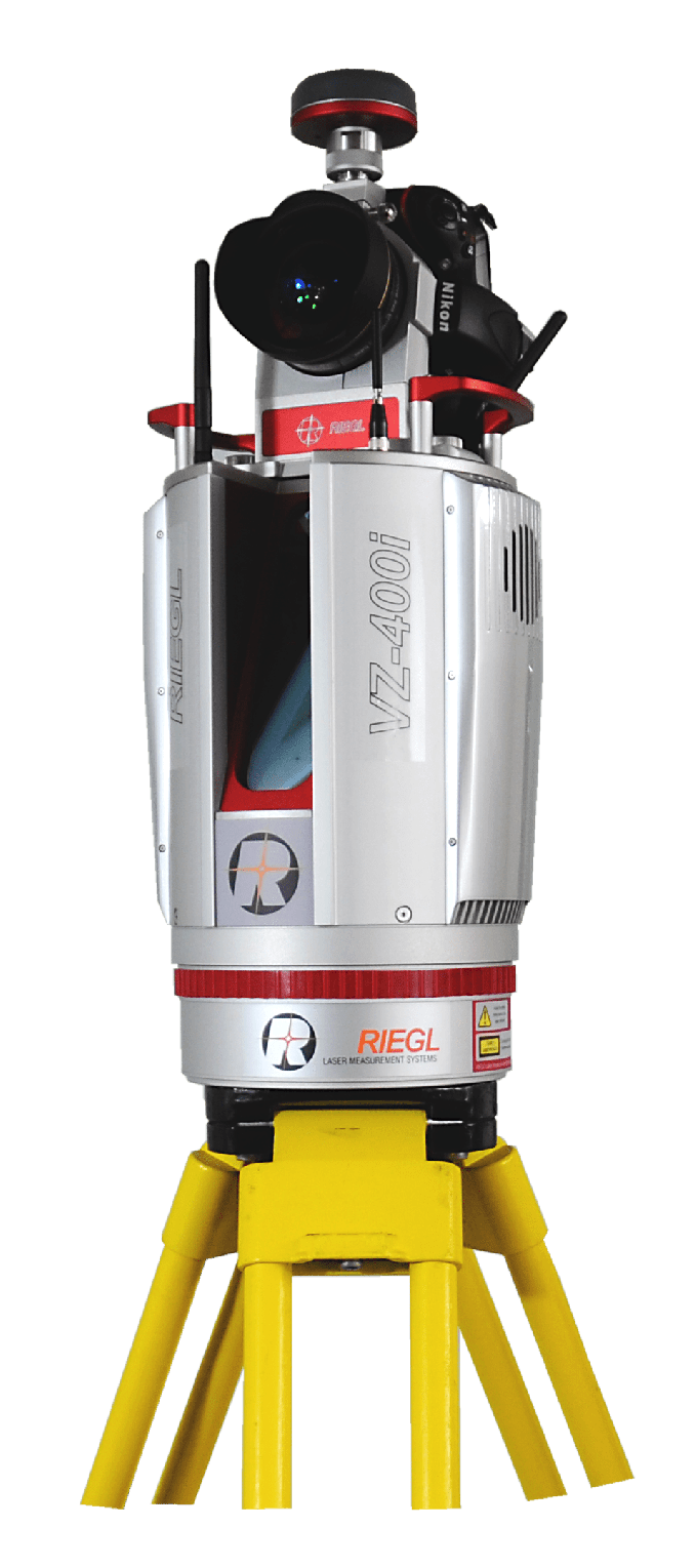
Figure 9.
TLS locations during the test measurements.

Figure 10.
Point cloud of the lab with the belt conveyor.

Figure 11.
Preliminary belt detection with an XGBoost Classifier.

Figure 12.
Belt detection enhanced with RANSAC plane fit.

Figure 13.
Original point cloud clipped to the belt bounding box.

Figure 14.
DBSCAN point cloud segmentation (main cluster in cyan).

Figure 15.
Final point cloud representing the belt surface.
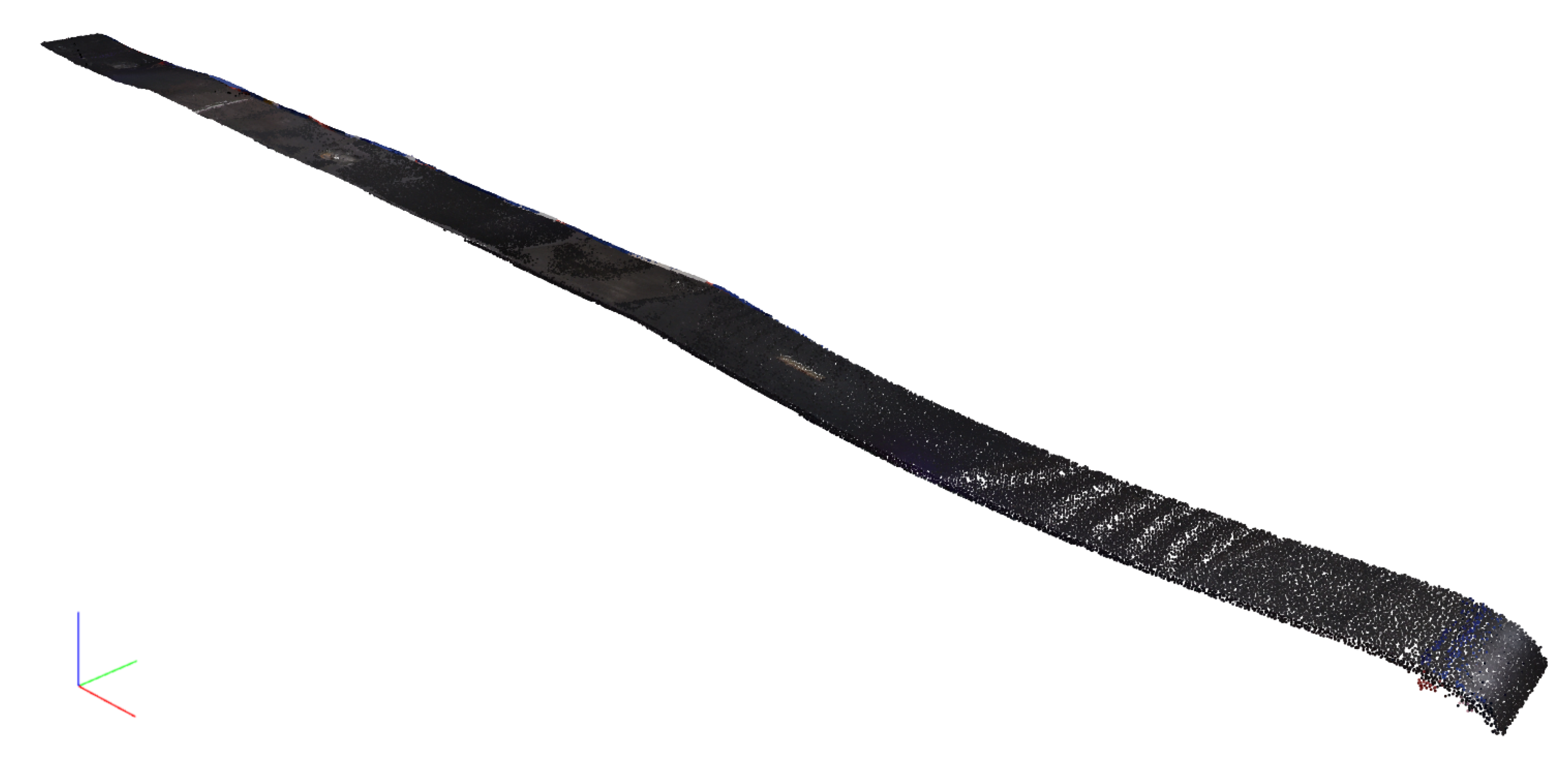
Figure 16.
Raster of relative belt surface elevation (values in meters).

Figure 17.
Estimation of local belt defects (values in meters).

Figure 18.
Segmented points representing belt longitudinal edges (in blue and green) and noise (in red).
Figure 18.
Segmented points representing belt longitudinal edges (in blue and green) and noise (in red).

Figure 19.
Line fit residuals of belt edges points.


Table 1.
3D shape features extracted from the neighborhood geometry [49].
Table 1.
3D shape features extracted from the neighborhood geometry [49].
| Local 3D Shape Descriptor | Definition |
|---|---|
| sum of eigenvalues | |
| planarity | |
| linearity | |
| anisotropy | |
| omnivariance | |
| eigenentropy | |
| first principal component | |
| second principal component | |
| third principal component (curvature) | |
| verticality |
Table 2.
Classification evaluation metrics.
| Class | Precision | Recall | |
|---|---|---|---|
| belt surface points | 0.992 | 0.983 | 0.988 |
| other points | 0.999 | 1.000 | 1.000 |
Publisher’s Note: MDPI stays neutral with regard to jurisdictional claims in published maps and institutional affiliations. |
© 2020 by the authors. Licensee MDPI, Basel, Switzerland. This article is an open access article distributed under the terms and conditions of the Creative Commons Attribution (CC BY) license (http://creativecommons.org/licenses/by/4.0/).
Share and Cite
MDPI and ACS Style
Trybała, P.; Blachowski, J.; Błażej, R.; Zimroz, R. Damage Detection Based on 3D Point Cloud Data Processing from Laser Scanning of Conveyor Belt Surface. Remote Sens. 2021, 13, 55. https://0-doi-org.brum.beds.ac.uk/10.3390/rs13010055
AMA Style
Trybała P, Blachowski J, Błażej R, Zimroz R. Damage Detection Based on 3D Point Cloud Data Processing from Laser Scanning of Conveyor Belt Surface. Remote Sensing. 2021; 13(1):55. https://0-doi-org.brum.beds.ac.uk/10.3390/rs13010055
Chicago/Turabian StyleTrybała, Paweł, Jan Blachowski, Ryszard Błażej, and Radosław Zimroz. 2021. "Damage Detection Based on 3D Point Cloud Data Processing from Laser Scanning of Conveyor Belt Surface" Remote Sensing 13, no. 1: 55. https://0-doi-org.brum.beds.ac.uk/10.3390/rs13010055
Note that from the first issue of 2016, this journal uses article numbers instead of page numbers. See further details here.