LaeNet: A Novel Lightweight Multitask CNN for Automatically Extracting Lake Area and Shoreline from Remote Sensing Images

 , , , , and
Abstract
:
1. Introduction
2. Study Area and Data
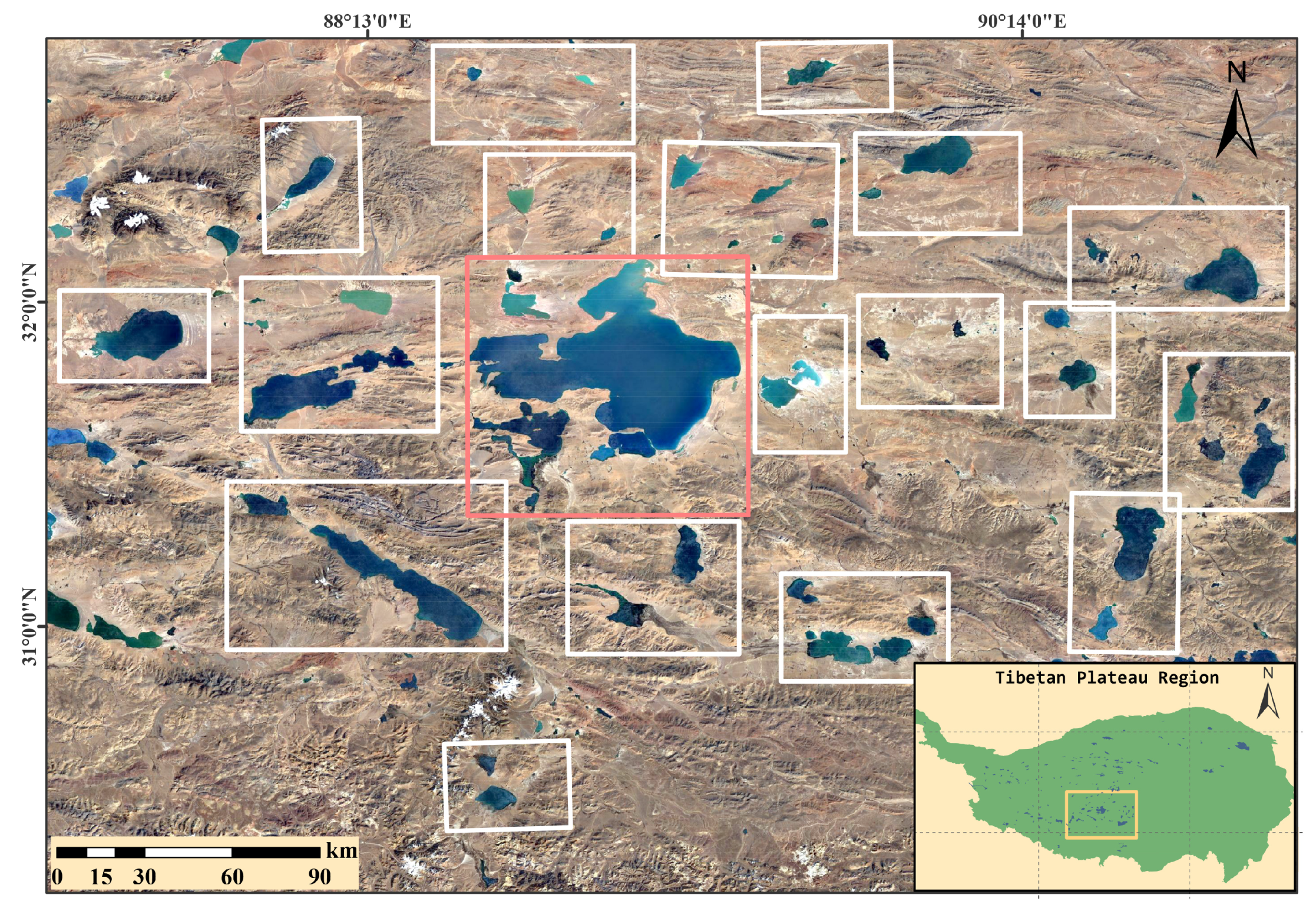
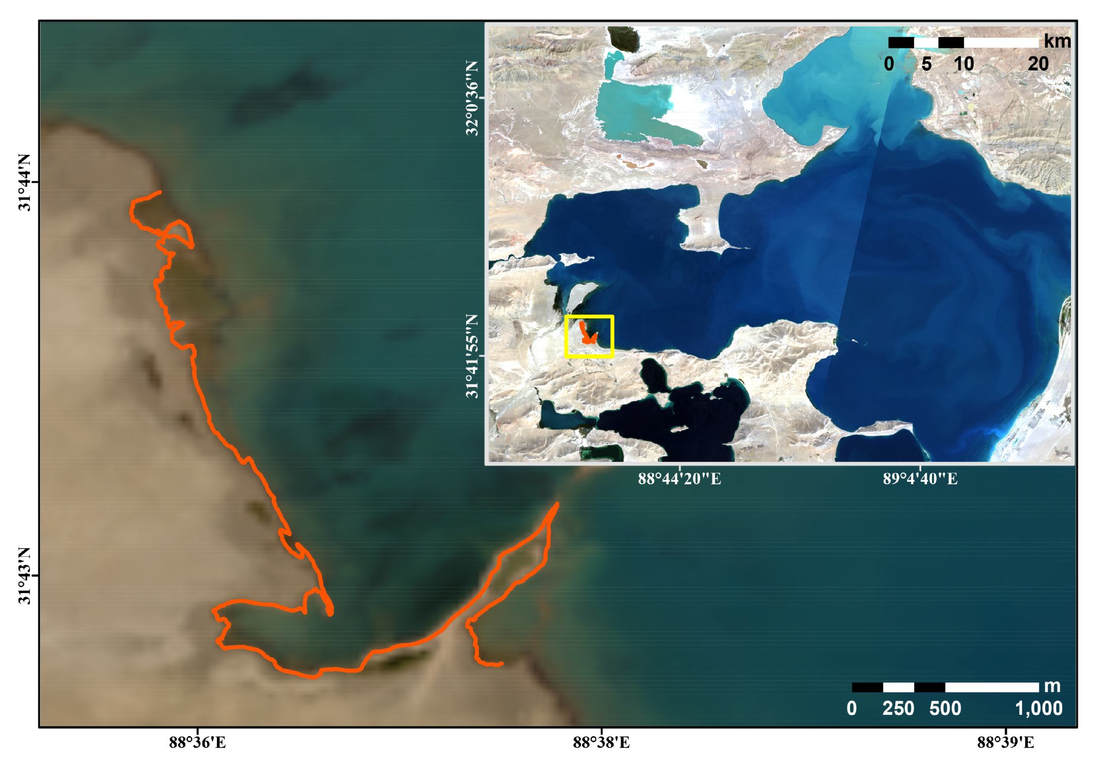
2.1. Study Area
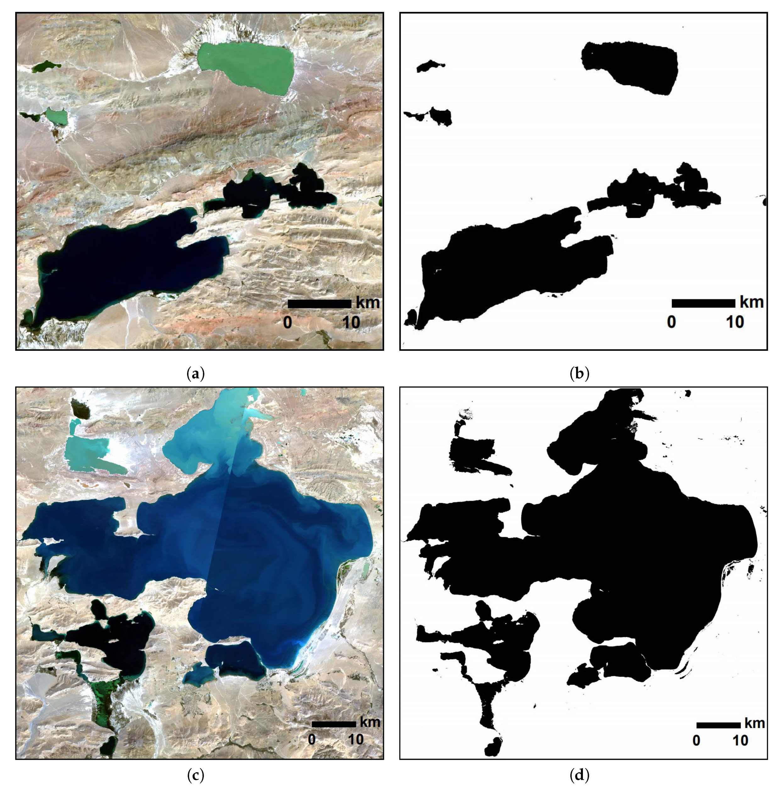
2.2. Landsat Images
2.3. Field-Measured Lakeshore from GPS
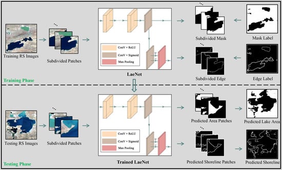
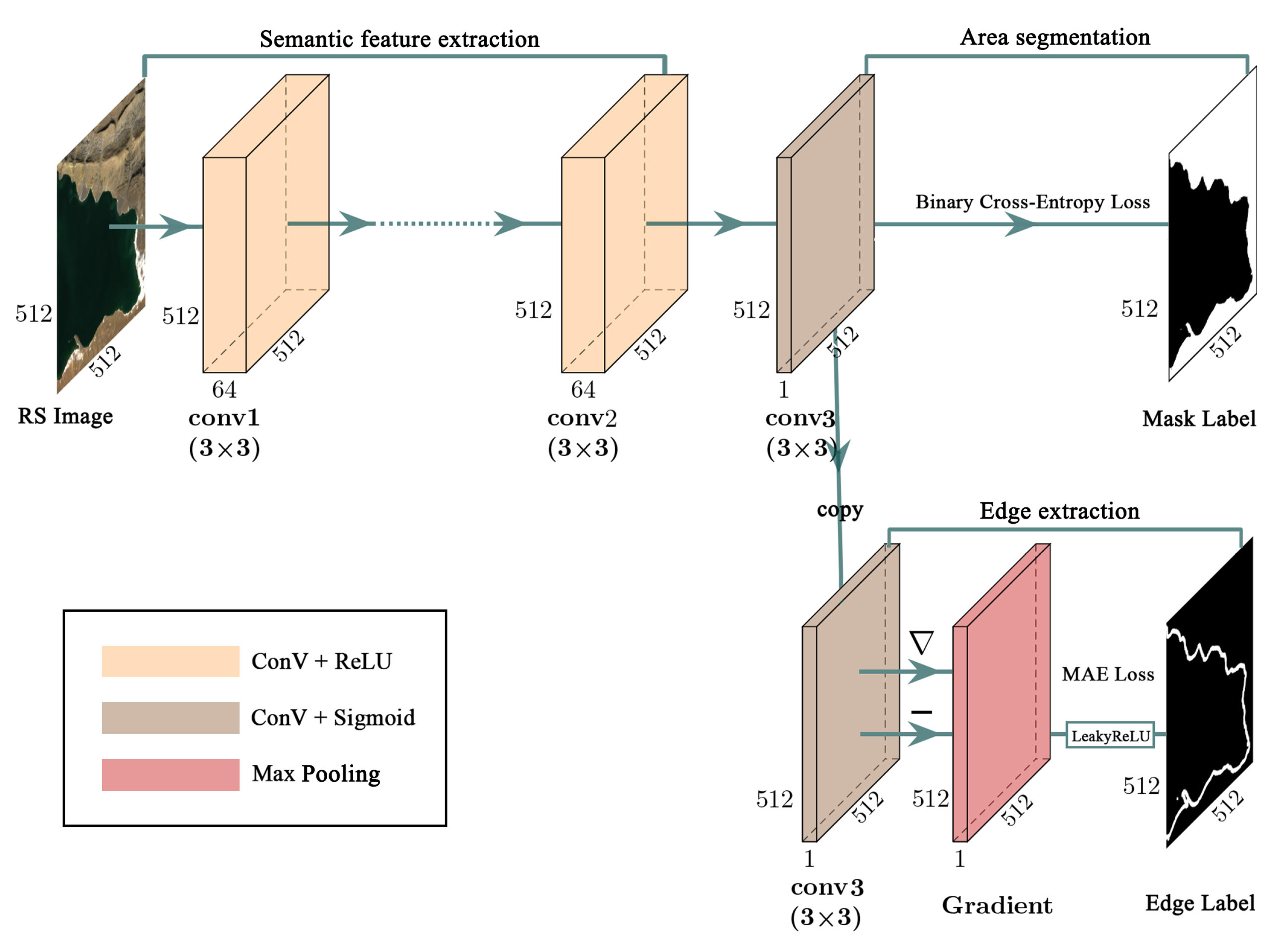
3. LaeNet Model
3.1. Semantic Feature Extraction
3.2. Area Segmentation
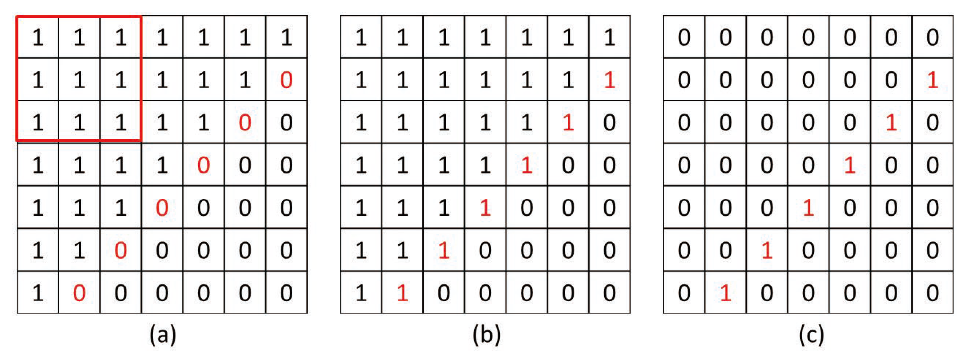
3.3. Edge Extraction
4. Results
4.1. Experimental Settings
4.2. Evaluation Criteria
4.3. Performance Comparison on Band Combination and Different CNN Layers
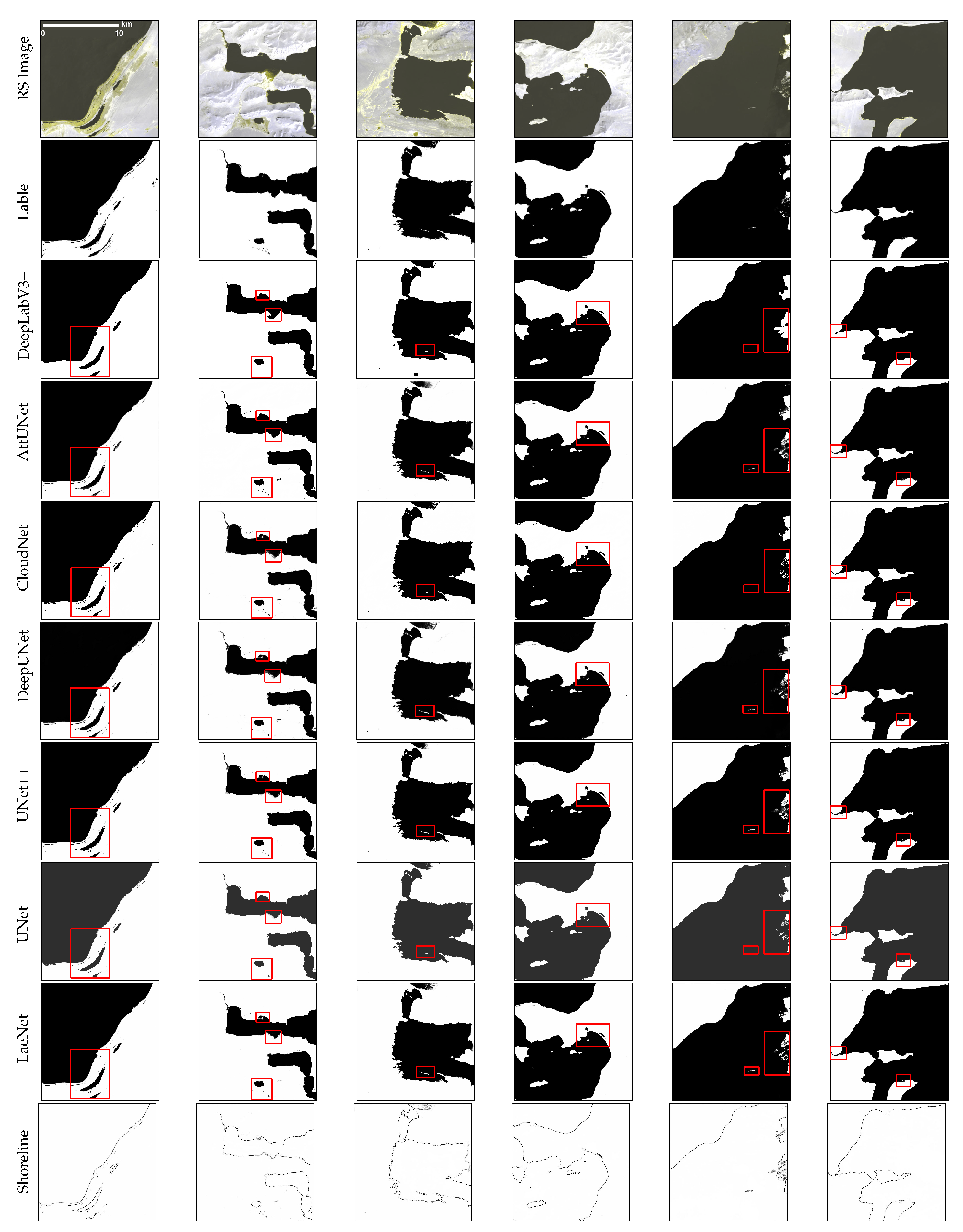
4.4. Performance Comparison with Different Semantic Segmentation Models
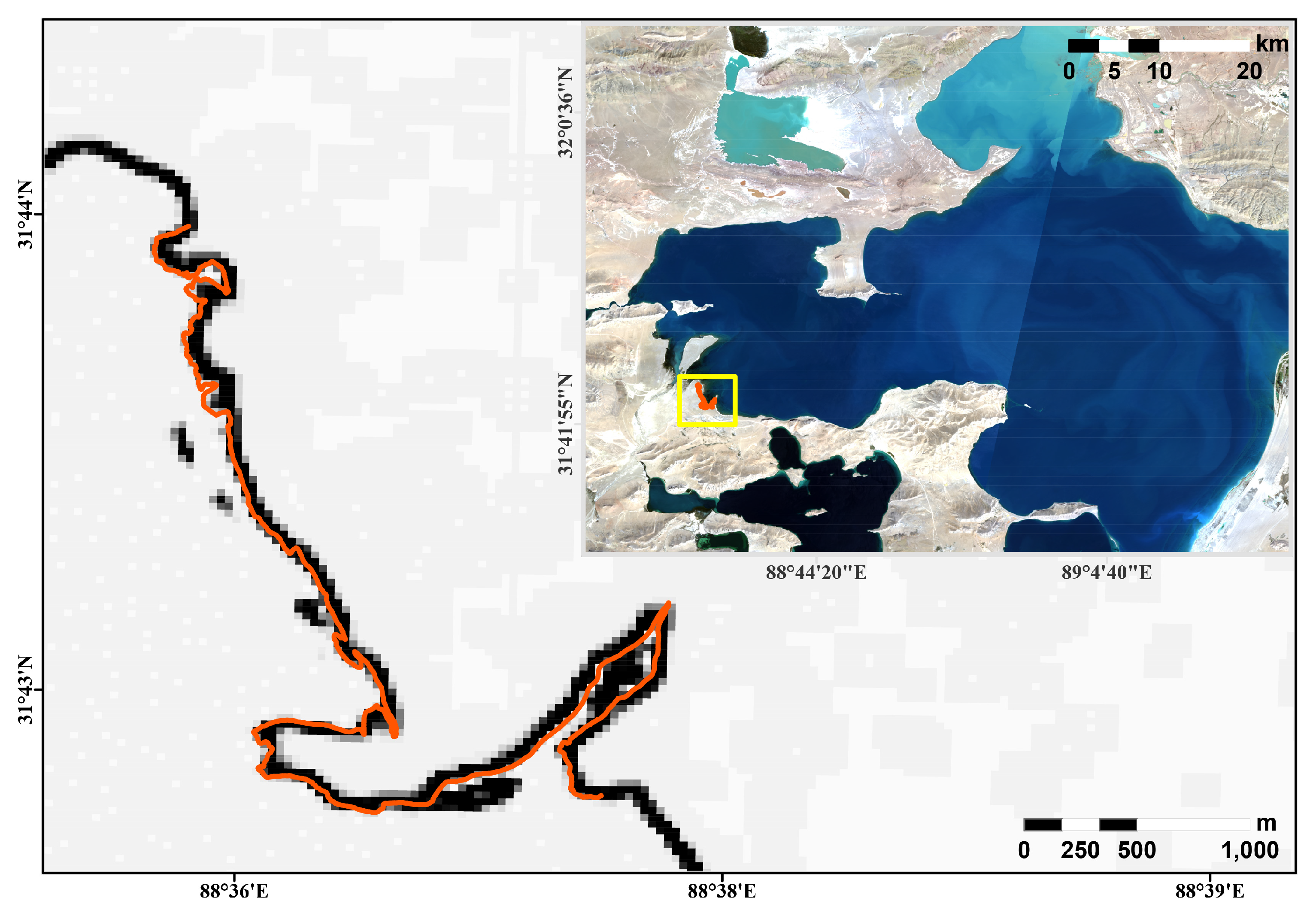
4.5. Performance Comparison with Situ Observed Results
5. Discussion
5.1. Applications on Different Attention Mechanisms
5.2. Effect of Pixel Tolerance on Different Semantic Segmentation Models
5.3. Applications on Images from Different Satellite Sensors
6. Conclusions
Author Contributions
Funding
Institutional Review Board Statement
Informed Consent Statement
Data Availability Statement
Acknowledgments
Conflicts of Interest
References
- Yang, K.; Ye, B.; Zhou, D.; Wu, B.; Foken, T.; Qin, J.; Zhou, Z. Response of hydrological cycle to recent climate changes in the Tibetan Plateau. Clim. Chang. 2011, 109, 517–534. [Google Scholar] [CrossRef]
- Zhu, L.; Wang, J.; Ju, J.; Ma, N.; Zhang, Y.; Liu, C.; Han, B.; Liu, L.; Wang, M.; Ma, Q. Climatic and lake environmental changes in the Serling Co region of Tibet over a variety of timescales. Sci. Bull. 2019, 64, 422–424. [Google Scholar] [CrossRef] [Green Version]
- Zhang, G.; Luo, W.; Chen, W.; Zheng, G. A robust but variable lake expansion on the Tibetan Plateau. Sci. Bull. 2019, 64, 1306–1309. [Google Scholar] [CrossRef] [Green Version]
- Zhang, G.; Yao, T.; Xie, H.; Yang, K.; Zhu, L.; Shum, C.; Bolch, T.; Yi, S.; Allen, S.; Jiang, L. Response of Tibetan Plateau’s lakes to climate changes: Trend, pattern, and mechanisms. Earth-Sci. Rev. 2020, 208, 103269. [Google Scholar] [CrossRef]
- Zhang, G.; Yao, T.; Shum, C.; Yi, S.; Yang, K.; Xie, H.; Feng, W.; Bolch, T.; Wang, L.; Behrangi, A. Lake volume and groundwater storage variations in Tibetan Plateau’s endorheic basin. Geophys. Res. Lett. 2017, 44, 5550–5560. [Google Scholar] [CrossRef]
- Song, C.; Huang, B.; Richards, K.; Ke, L.; Hien Phan, V. Accelerated lake expansion on the Tibetan Plateau in the 2000s: Induced by glacial melting or other processes? Water Resour. Res. 2014, 50, 3170–3186. [Google Scholar] [CrossRef] [Green Version]
- Ma, N.; Szilagyi, J.; Niu, G.Y.; Zhang, Y.; Zhang, T.; Wang, B.; Wu, Y. Evaporation variability of Nam Co Lake in the Tibetan Plateau and its role in recent rapid lake expansion. J. Hydrol. 2016, 537, 27–35. [Google Scholar] [CrossRef]
- Duru, U. Shoreline change assessment using multi-temporal satellite images: A case study of Lake Sapanca, NW Turkey. Environ. Monit. Assess. 2017, 189, 385. [Google Scholar] [CrossRef]
- Li, X.; Long, D.; Huang, Q.; Han, P.; Zhao, F.; Wada, Y. High-temporal-resolution water level and storage change data sets for lakes on the Tibetan Plateau during 2000–2017 using multiple altimetric missions and Landsat-derived lake shoreline positions. Earth Syst. Sci. Data Discuss. 2019, 11, 1603–1627. [Google Scholar] [CrossRef] [Green Version]
- Qiao, B.; Zhu, L.; Yang, R. Temporal-spatial differences in lake water storage changes and their links to climate change throughout the Tibetan Plateau. Remote Sens. Environ. 2019, 222, 232–243. [Google Scholar] [CrossRef]
- Zhang, G.; Xie, H.; Kang, S.; Yi, D.; Ackley, S.F. Monitoring lake level changes on the Tibetan Plateau using ICESat altimetry data (2003–2009). Remote Sens. Environ. 2011, 115, 1733–1742. [Google Scholar] [CrossRef]
- Lei, Y.; Yao, T.; Yang, K.; Sheng, Y.; Kleinherenbrink, M.; Yi, S.; Bird, B.W.; Zhang, X.; Zhu, L.; Zhang, G. Lake seasonality across the Tibetan Plateau and their varying relationship with regional mass changes and local hydrology. Geophys. Res. Lett. 2017, 44, 892–900. [Google Scholar] [CrossRef] [Green Version]
- Wang, H.; Chu, Y.; Huang, Z.; Hwang, C.; Chao, N. Robust, long-term lake level change from multiple satellite altimeters in Tibet: Observing the rapid rise of Ngangzi Co over a new wetland. Remote Sens. 2019, 11, 558. [Google Scholar] [CrossRef] [Green Version]
- Zhang, G.; Yao, T.; Xie, H.; Wang, W.; Yang, W. An inventory of glacial lakes in the Third Pole region and their changes in response to global warming. Glob. Planet. Chang. 2015, 131, 148–157. [Google Scholar] [CrossRef]
- Ye, Q.; Zhu, L.; Zheng, H.; Naruse, R.; Zhang, X.; Kang, S. Glacier and lake variations in the Yamzhog Yumco basin, southern Tibetan Plateau, from 1980 to 2000 using remote-sensing and GIS technologies. J. Glaciol. 2007, 53, 673–676. [Google Scholar] [CrossRef] [Green Version]
- El-Asmar, H.M.; Hereher, M.E.; El Kafrawy, S.B. Surface area change detection of the Burullus Lagoon, North of the Nile Delta, Egypt, using water indices: A remote sensing approach. Egypt. J. Remote Sens. Space Sci. 2013, 16, 119–123. [Google Scholar] [CrossRef] [Green Version]
- Lu, S.; Ouyang, N.; Wu, B.; Wei, Y.; Tesemma, Z. Lake water volume calculation with time series remote-sensing images. Int. J. Remote Sens. 2013, 34, 7962–7973. [Google Scholar] [CrossRef]
- Bolch, T.; Buchroithner, M.F.; Peters, J.; Baessler, M.; Bajracharya, S. Identification of glacier motion and potentially dangerous glacial lakes in the Mt. Everest region/Nepal using spaceborne imagery. Nat. Hazards Earth Syst. Sci. 2008, 8, 1329–1340. [Google Scholar] [CrossRef] [Green Version]
- Salerno, F.; Thakuri, S.; D’Agata, C.; Smiraglia, C.; Manfredi, E.C.; Viviano, G.; Tartari, G. Glacial lake distribution in the Mount Everest region: Uncertainty of measurement and conditions of formation. Glob. Planet. Chang. 2012, 92, 30–39. [Google Scholar] [CrossRef]
- Wang, X.; Ding, Y.; Liu, S.; Jiang, L.; Wu, K.; Jiang, Z.; Guo, W. Changes of glacial lakes and implications in Tian Shan, central Asia, based on remote sensing data from 1990 to 2010. Environ. Res. Lett. 2013, 8, 044052. [Google Scholar] [CrossRef]
- Incekara, A.H.; Seker, D.Z.; Bayram, B. Qualifying the LIDAR-Derived Intensity Image as an Infrared Band in NDWI-Based Shoreline Extraction. IEEE J. Sel. Top. Appl. Earth Obs. Remote Sens. 2018, 11, 5053–5062. [Google Scholar] [CrossRef]
- Ding, X.; Li, X. Shoreline movement monitoring based on SAR images in Shanghai, China. Int. J. Remote Sens. 2014, 35, 3994–4008. [Google Scholar] [CrossRef]
- Shandi, Z.; Helali, H. Investigation of 2019 Rainfall Effects on Urmia Lake Surface and Extraction of Lake Shoreline Changes and Comparison with the Previous Decade Using Remote Sensing Images and GIS. Isprs J. Photogramm. Remote Sens. 2020, 43, 759–766. [Google Scholar] [CrossRef]
- McFeeters, S.K. The use of the Normalized Difference Water Index (NDWI) in the delineation of open water features. Int. J. Remote Sens. 1996, 17, 1425–1432. [Google Scholar] [CrossRef]
- Xu, H. Modification of normalised difference water index (NDWI) to enhance open water features in remotely sensed imagery. Int. J. Remote Sens. 2006, 27, 3025–3033. [Google Scholar] [CrossRef]
- Li, B.; Yang, G.; Wan, R.; Dai, X.; Zhang, Y. Comparison of random forests and other statistical methods for the prediction of lake water level: A case study of the Poyang Lake in China. Nord. Hydrol. 2016, 47, 69–83. [Google Scholar] [CrossRef] [Green Version]
- Khan, M.S.; Coulibaly, P. Application of support vector machine in lake water level prediction. J. Hydrol. Eng. 2006, 11, 199–205. [Google Scholar] [CrossRef]
- Yadav, B.; Eliza, K. A hybrid wavelet-support vector machine model for prediction of lake water level fluctuations using hydro-meteorological data. Measurement 2017, 103, 294–301. [Google Scholar] [CrossRef]
- Minghelli, A.; Spagnoli, J.; Lei, M.; Chami, M.; Charmasson, S. Shoreline Extraction from WorldView2 Satellite Data in the Presence of Foam Pixels Using Multispectral Classification Method. Remote Sens. 2020, 12, 2664. [Google Scholar] [CrossRef]
- Altunkaynak, A. Forecasting surface water level fluctuations of Lake Van by artificial neural networks. Water Resour. Manag. 2007, 21, 399–408. [Google Scholar] [CrossRef]
- Kisi, O.; Shiri, J.; Nikoofar, B. Forecasting daily lake levels using artificial intelligence approaches. Comput. Geosci. 2012, 41, 169–180. [Google Scholar] [CrossRef]
- Young, C.C.; Liu, W.C.; Hsieh, W.L. Predicting the water level fluctuation in an alpine lake using physically based, artificial neural network, and time series forecasting models. Math. Probl. Eng. 2015, 2015. [Google Scholar] [CrossRef] [Green Version]
- Feng, Z.; Huang, G.; Chi, D. Classification of the Complex Agricultural Planting Structure with a Semi-Supervised Extreme Learning Machine Framework. Remote Sens. 2020, 12, 3708. [Google Scholar] [CrossRef]
- Demir, N.; Bayram, B.; Şeker, D.Z.; Oy, S.; İnce, A.; Bozkurt, S. Advanced lake shoreline extraction approach by integration of SAR image and LIDAR data. Mar. Geodesy 2019, 42, 166–185. [Google Scholar] [CrossRef]
- LeCun, Y.; Bengio, Y.; Hinton, G. Deep learning. Nature 2015, 521, 436–444. [Google Scholar] [CrossRef]
- Reichstein, M.; Camps-Valls, G.; Stevens, B.; Jung, M.; Denzler, J.; Carvalhais, N. Deep learning and process understanding for data-driven Earth system science. Nature 2019, 566, 195–204. [Google Scholar] [CrossRef]
- Yuan, J.; Chi, Z.; Cheng, X.; Zhang, T.; Li, T.; Chen, Z. Automatic Extraction of Supraglacial Lakes in Southwest Greenland during the 2014–2018 Melt Seasons Based on Convolutional Neural Network. Water 2020, 12, 891. [Google Scholar] [CrossRef] [Green Version]
- Liang, C.; Li, H.; Lei, M.; Du, Q. Dongting lake water level forecast and its relationship with the three gorges dam based on a long short-term memory network. Water 2018, 10, 1389. [Google Scholar] [CrossRef] [Green Version]
- Pu, F.; Ding, C.; Chao, Z.; Yu, Y.; Xu, X. Water-quality classification of inland lakes using landsat8 images by convolutional neural networks. Remote Sens. 2019, 11, 1674. [Google Scholar] [CrossRef] [Green Version]
- Rostami, M.; Kolouri, S.; Eaton, E.; Kim, K. Deep transfer learning for few-shot sar image classification. Remote Sens. 2019, 11, 1374. [Google Scholar] [CrossRef] [Green Version]
- Ren, Y.; Zhang, X.; Ma, Y.; Yang, Q.; Wang, C.; Liu, H.; Qi, Q. Full Convolutional Neural Network Based on Multi-Scale Feature Fusion for the Class Imbalance Remote Sensing Image Classification. Remote Sens. 2020, 12, 3547. [Google Scholar] [CrossRef]
- Mostajabi, M.; Yadollahpour, P.; Shakhnarovich, G. Feedforward semantic segmentation with zoom-out features. In Proceedings of the IEEE Conference on Computer Vision and Pattern Recognition, Boston, MA, USA, 7–12 June 2015; pp. 3376–3385. [Google Scholar]
- Eigen, D.; Fergus, R. Predicting depth, surface normals and semantic labels with a common multi-scale convolutional architecture. In Proceedings of the IEEE Conference on Computer Vision and Pattern Recognition, Boston, MA, USA, 7–12 June 2015; pp. 2650–2658. [Google Scholar]
- Li, L. Deep Residual Autoencoder with Multiscaling for Semantic Segmentation of Land-Use Images. Remote Sens. 2019, 11, 2142. [Google Scholar] [CrossRef] [Green Version]
- Wang, J.; HQ Ding, C.; Chen, S.; He, C.; Luo, B. Semi-Supervised Remote Sensing Image Semantic Segmentation via Consistency Regularization and Average Update of Pseudo-Label. Remote Sens. 2020, 12, 3603. [Google Scholar] [CrossRef]
- Zhang, E.; Liu, L.; Huang, L. Automatically delineating the calving front of Jakobshavn Isbræ from multitemporal TerraSAR-X images: A deep learning approach. Cryosphere 2019, 13, 1729–1741. [Google Scholar] [CrossRef] [Green Version]
- Huang, L.; Liu, L.; Jiang, L.; Zhang, T. Automatic mapping of thermokarst landforms from remote sensing images using deep learning: A case study in the Northeastern Tibetan Plateau. Remote Sens. 2018, 10, 2067. [Google Scholar] [CrossRef] [Green Version]
- Chen, L.C.; Papandreou, G.; Kokkinos, I.; Murphy, K.; Yuille, A.L. Semantic image segmentation with deep convolutional nets and fully connected crfs. arXiv 2014, arXiv:1412.7062. [Google Scholar]
- Qin, M.; Hu, L.; Du, Z.; Gao, Y.; Qin, L.; Zhang, F.; Liu, R. Achieving Higher Resolution Lake Area from Remote Sensing Images Through an Unsupervised Deep Learning Super-Resolution Method. Remote Sens. 2020, 12, 1937. [Google Scholar] [CrossRef]
- Liu, S.; Ding, W.; Liu, C.; Liu, Y.; Wang, Y.; Li, H. ERN: Edge loss reinforced semantic segmentation network for remote sensing images. Remote Sens. 2018, 10, 1339. [Google Scholar] [CrossRef] [Green Version]
- Ronneberger, O.; Fischer, P.; Brox, T. U-net: Convolutional networks for biomedical image segmentation. In Proceedings of the International Conference on Medical Image Computing and Computer-Assisted Intervention, Munich, Germany, 5–9 October 2015; pp. 234–241. [Google Scholar]
- Waldner, F.; Diakogiannis, F.I. Deep learning on edge: Extracting field boundaries from satellite images with a convolutional neural network. Remote Sens. Environ. 2020, 245, 111741. [Google Scholar] [CrossRef]
- Diakogiannis, F.I.; Waldner, F.; Caccetta, P.; Wu, C. Resunet-a: A deep learning framework for semantic segmentation of remotely sensed data. ISPRS J. Photogramm. Remote Sens. 2020, 162, 94–114. [Google Scholar] [CrossRef] [Green Version]
- Chen, L.C.; Zhu, Y.; Papandreou, G.; Schroff, F.; Adam, H. Encoder-decoder with atrous separable convolution for semantic image segmentation. In Proceedings of the European Conference on Computer Vision (ECCV), Munich, Germany, 8–14 September 2018; pp. 801–818. [Google Scholar]
- Huang, L.; Luo, J.; Lin, Z.; Niu, F.; Liu, L. Using deep learning to map retrogressive thaw slumps in the Beiluhe region (Tibetan Plateau) from CubeSat images. Remote Sens. Environ. 2020, 237, 111534. [Google Scholar] [CrossRef]
- Liu, X.; Chen, B. Climatic warming in the Tibetan Plateau during recent decades. Int. J. Climatol. 2000, 20, 1729–1742. [Google Scholar] [CrossRef]
- Zhang, Y.; Yao, T.; Ma, Y. Climatic changes have led to significant expansion of endorheic lakes in Xizang (Tibet) since 1995. Sci. Cold Arid Reg. 2011, 3, 0463–0467. [Google Scholar]
- Zhou, J.; Wang, L.; Zhang, Y.; Guo, Y.; Li, X.; Liu, W. Exploring the water storage changes in the largest lake (S elin C o) over the T ibetan P lateau during 2003–2012 from a basin-wide hydrological modeling. Water Resour. Res. 2015, 51, 8060–8086. [Google Scholar] [CrossRef] [Green Version]
- Takasu, T.; Yasuda, A. Kalman-filter-based integer ambiguity resolution strategy for long-baseline RTK with ionosphere and troposphere estimation. In Proceedings of the ION GNSS, Portland, OR, USA, 21–24 September 2010; pp. 161–171. [Google Scholar]
- Xu, N.; Price, B.; Cohen, S.; Huang, T. Deep image matting. In Proceedings of the IEEE Conference on Computer Vision and Pattern Recognition, Honolulu, HI, USA, 21–26 July 2017; pp. 2970–2979. [Google Scholar]
- Zhen, M.; Wang, J.; Zhou, L.; Li, S.; Shen, T.; Shang, J.; Fang, T.; Quan, L. Joint Semantic Segmentation and Boundary Detection using Iterative Pyramid Contexts. In Proceedings of the IEEE Conference on Computer Vision and Pattern Recognition, Seattle, WA, USA, 14–19 June 2020; pp. 13666–13675. [Google Scholar]
- Kingma, D.; Ba, J. Adam: A Method for Stochastic Optimization. arXiv 2014, arXiv:1412.6980. [Google Scholar]
- Ozan, O.; Jo, S.; Loic, L.F.; Matthew, L.; Mattias, H.; Kazunari, M.; Kensaku, M.; Steven, M.; Nils Y, H.; Bernhard, K.; et al. Attention U-Net: Learning Where to Look for the Pancreas. arXiv 2018, arXiv:1810.03999. [Google Scholar]
- Mohajerani, S.; Saeedi, P. Cloud-Net: An end-to-end cloud detection algorithm for Landsat 8 imagery. In Proceedings of the IGARSS 2019-2019 IEEE International Geoscience and Remote Sensing Symposium, Yokohama, Japan, 28 July–2 August 2019; pp. 1029–1032. [Google Scholar]
- Li, R.; Liu, W.; Yang, L.; Sun, S.; Hu, W.; Zhang, F.; Li, W. Deepunet: A deep fully convolutional network for pixel-level sea-land segmentation. IEEE J. Sel. Top Appl. Earth Obs. Remote Sens. 2018, 11, 3954–3962. [Google Scholar] [CrossRef] [Green Version]
- Zhou, Z.; Siddiquee, M.M.R.; Tajbakhsh, N.; Liang, J. UNet++: Redesigning Skip Connections to Exploit Multiscale Features in Image Segmentation. IEEE Trans. Med. Imaging 2019, 6, 1856–1867. [Google Scholar] [CrossRef] [Green Version]
- Zhou, Z.; Siddiquee, M.M.R.; Tajbakhsh, N.; Liang, J. Unet++: A Nested U-Net Architecture for Medical Image Segmentation. In Deep Learning in Medical Image Analysis and Multimodal Learning for Clinical Decision Support; Springer: Berlin/Heidelberg, Germany, 2018; pp. 3–11. [Google Scholar]
- Chollet, F. Xception: Deep learning with depthwise separable convolutions. In Proceedings of the IEEE Conference on Computer Vision and Pattern Recognition, Honolulu, HI, USA, 21–26 July 2017; pp. 1251–1258. [Google Scholar]
- Russakovsky, O.; Deng, J.; Su, H.; Krause, J.; Satheesh, S.; Ma, S.; Huang, Z.; Karpathy, A.; Khosla, A. Imagenet large scale visual recognition challenge. Int. J. Comput. Vis. 2015, 115, 211–252. [Google Scholar] [CrossRef] [Green Version]
- Mohajerani, S.; Saeedi, P. Shadow Detection in Single RGB Images Using a Context Preserver Convolutional Neural Network Trained by Multiple Adversarial Examples. IEEE Trans. Image Process 2019, 28, 4117–4129. [Google Scholar] [CrossRef]
- Mou, L.; Zhu, X.X. Learning to pay attention on spectral domain: A spectral attention module-based convolutional network for hyperspectral image classification. IEEE Trans. Geosci. Remote Sens. 2019, 58, 110–122. [Google Scholar] [CrossRef]
- Woo, S.; Park, J.; Lee, J.Y.; So Kweon, I. Cbam: Convolutional block attention module. In Proceedings of the European conference on computer vision (ECCV), Munich, Germany, 8–14 September 2018; pp. 3–19. [Google Scholar]
- Qiao, Y.; Liu, Y.; Yang, X.; Zhou, D.; Xu, M.; Zhang, Q.; Wei, X. Attention-Guided Hierarchical Structure Aggregation for Image Matting. In Proceedings of the IEEE Conference on Computer Vision and Pattern Recognition, Seattle, WA, USA, 14–19 June 2020; pp. 13676–13685. [Google Scholar]
- Augustauskas, R.; Lipnickas, A. Improved Pixel-Level Pavement-Defect Segmentation Using a Deep Autoencoder. Sensors 2020, 20, 2557. [Google Scholar] [CrossRef] [PubMed]
- Lau, S.L.; Wang, X.; Xu, Y.; Chong, E.K. Automated Pavement Crack Segmentation Using Fully Convolutional U-Net with a Pretrained ResNet-34 Encoder. arXiv 2020, arXiv:2001.01912. [Google Scholar]
- Escalona, U.; Arce, F.; Zamora, E.; Sossa Azuela, J.H. Fully convolutional networks for automatic pavement crack segmentation. Comput. Sist. 2019, 23, 451–460. [Google Scholar] [CrossRef]


| Landsat-5 | Landsat-8 | ||||
|---|---|---|---|---|---|
| BandName | WaveLength (m) | Resolution (m) | BandName | WaveLength (m) | Resolution (m) |
| B1(Blue) | 0.45–0.52 | 30 | B2(Blue) | 0.45–0.51 | 30 |
| B2(Green) | 0.52–0.60 | 30 | B3(Green) | 0.53–0.59 | 30 |
| B3(Red) | 0.63–0.69 | 30 | B4(Red) | 0.64–0.67 | 30 |
| B4(NIR) | 0.76–0.90 | 30 | B5(NIR) | 0.85–0.88 | 30 |
| B5(SWIR) | 1.55–1.75 | 30 | B6(SWIR) | 1.57–1.65 | 30 |
| Band | 1 Layer | 2 Layers | 3 Layers |
|---|---|---|---|
| B2 | 0.2331 | 0.2331 | 0.2331 |
| B3 | 0.2331 | 0.2331 | 0.2331 |
| B4 | 0.8971 | 0.8471 | 0.8520 |
| B5 | 0.9832 | 0.9826 | 0.9823 |
| B6 | 0.9855 | 0.9855 | 0.9854 |
| B2 + B3 | 0.8202 | 0.8224 | 0.8396 |
| B2 + B4 | 0.9606 | 0.9574 | 0.9636 |
| B2 + B5 | 0.9837 | 0.9831 | 0.9837 |
| B2 + B5 | 0.9850 | 0.9768 | 0.9827 |
| B3 + B4 | 0.9756 | 0.9756 | 0.9755 |
| B3 + B5 | 0.9838 | 0.9843 | 0.9841 |
| B3 + B6 | 0.9844 | 0.9838 | 0.9829 |
| B4 + B5 | 0.9848 | 0.9839 | 0.9845 |
| B4 + B6 | 0.9848 | 0.9851 | 0.9843 |
| B5 + B6 | 0.9879 | 0.9875 | 0.9867 |
| B2 + B3 + B4 | 0.9747 | 0.9752 | 0.9755 |
| B2 + B3 + B5 | 0.9853 | 0.9836 | 0.9820 |
| B2 + B3 + B6 | 0.9841 | 0.9846 | 0.9840 |
| B2 + B4 + B5 | 0.9853 | 0.9841 | 0.9840 |
| B2 + B4 + B6 | 0.9847 | 0.9844 | 0.9840 |
| B2 + B5 + B6 | 0.9865 | 0.9862 | 0.9857 |
| B3 + B4 + B5 | 0.9849 | 0.9838 | 0.9847 |
| B3 + B4 + B6 | 0.9846 | 0.9843 | 0.9828 |
| B3 + B5 + B6 | 0.9869 | 0.9854 | 0.9856 |
| B4 + B5 + B6 | 0.9873 | 0.9860 | 0.9853 |
| B2 + B3 + B4 + B5 | 0.9847 | 0.9836 | 0.9838 |
| B2 + B3 + B4 + B6 | 0.9838 | 0.9839 | 0.9833 |
| B2 + B3 + B5 + B6 | 0.9858 | 0.9858 | 0.9846 |
| B2 + B4 + B5 + B6 | 0.9866 | 0.9860 | 0.9850 |
| B3 + B4 + B5 + B6 | 0.9861 | 0.9855 | 0.9854 |
| ALL | 0.9852 | 0.9857 | 0.9856 |
| Model | Accuracy | Precision | Recall | F1-Score | mIoU | MSE | MAE | Time | Size |
|---|---|---|---|---|---|---|---|---|---|
| DeepLabV3+ | 0.9711 | 0.9440 | 0.9976 | 0.9701 | 0.9474 | 0.0488 | 0.0536 | 3′09″ | 329.2 MB |
| AttUNet | 0.9960 | 0.9581 | 0.9628 | 0.9604 | 0.9650 | 0.0033 | 0.0048 | 1′55″ | 95.1 MB |
| CloudNet | 0.9962 | 0.9579 | 0.9644 | 0.9611 | 0.9652 | 0.0035 | 0.0038 | 2′46″ | 438.1 MB |
| DeepUNet | 0.9958 | 0.9898 | 0.9955 | 0.9926 | 0.9857 | 0.0038 | 0.0087 | 0′28″ | 416.1 MB |
| UNet++ | 0.9960 | 0.9883 | 0.9986 | 0.9933 | 0.9864 | 0.0035 | 0.0058 | 0′53″ | 27.4 MB |
| UNet | 0.9961 | 0.9907 | 0.9975 | 0.9939 | 0.9875 | 0.0036 | 0.0057 | 1′52″ | 372.6 MB |
| LaeNet | 0.9962 | 0.9912 | 0.9982 | 0.9941 | 0.9879 | 0.0033 | 0.0046 | 0′06″ | 0.047 MB |
| Band | Accuracy | Precision | Recall | F1-Score | mIoU |
|---|---|---|---|---|---|
| ALL | 0.9959 | 0.9901 | 0.9961 | 0.9930 | 0.9863 |
| ALL + spectral attention | 0.9960 | 0.9894 | 0.9971 | 0.9932 | 0.9867 |
| ALL + channel attention | 0.9960 | 0.9911 | 0.9960 | 0.9935 | 0.9869 |
| B5+B6 | 0.9962 | 0.9912 | 0.9982 | 0.9941 | 0.9879 |
| Model | Tolerance in Pixels | Accuracy | Precision | Recall | F1-Score | mIoU |
|---|---|---|---|---|---|---|
| 0 | 0.9531 | 0.9901 | 0.9181 | 0.9340 | 0.9166 | |
| 1 | 0.9529 | 0.9944 | 0.9183 | 0.9357 | 0.9051 | |
| DeepLabV3+ | 2 | 0.9526 | 0.9978 | 0.9183 | 0.9374 | 0.9016 |
| 3 | 0.9513 | 0.9989 | 0.9155 | 0.9366 | 0.8958 | |
| 4 | 0.9498 | 0.9992 | 0.9118 | 0.9349 | 0.8899 | |
| 0 | 0.9938 | 0.9981 | 0.9531 | 0.9668 | 0.9384 | |
| 1 | 0.9931 | 0.9990 | 0.9533 | 0.9672 | 0.9248 | |
| AttUNet | 2 | 0.9921 | 0.9996 | 0.9519 | 0.9668 | 0.9194 |
| 3 | 0.9904 | 0.9997 | 0.9482 | 0.9649 | 0.9128 | |
| 4 | 0.9885 | 0.9998 | 0.9439 | 0.9626 | 0.9064 | |
| 0 | 0.9933 | 0.9968 | 0.9516 | 0.9622 | 0.9346 | |
| 1 | 0.9934 | 0.9983 | 0.9513 | 0.9627 | 0.9204 | |
| CloudNet | 2 | 0.9921 | 0.9990 | 0.9493 | 0.9621 | 0.9138 |
| 3 | 0.9903 | 0.9993 | 0.9453 | 0.9602 | 0.9129 | |
| 4 | 0.9884 | 0.9993 | 0.9407 | 0.9578 | 0.9052 | |
| 0 | 0.9933 | 0.9979 | 0.9518 | 0.9663 | 0.9361 | |
| 1 | 0.9928 | 0.9991 | 0.9526 | 0.9672 | 0.9234 | |
| DeepUNet | 2 | 0.9922 | 0.9996 | 0.9529 | 0.9677 | 0.9195 |
| 3 | 0.9906 | 0.9996 | 0.9494 | 0.9639 | 0.9070 | |
| 4 | 0.9888 | 0.9996 | 0.9453 | 0.9639 | 0.9070 | |
| 0 | 0.9939 | 0.9985 | 0.9533 | 0.9664 | 0.9393 | |
| 1 | 0.9930 | 0.9993 | 0.9523 | 0.9662 | 0.9243 | |
| UNet++ | 2 | 0.9918 | 0.9996 | 0.9503 | 0.9653 | 0.9184 |
| 3 | 0.9901 | 0.9997 | 0.9464 | 0.9633 | 0.9116 | |
| 4 | 0.9883 | 0.9997 | 0.9422 | 0.9610 | 0.9053 | |
| 0 | 0.9941 | 0.9990 | 0.9530 | 0.9658 | 0.9397 | |
| 1 | 0.9931 | 0.9997 | 0.9520 | 0.9656 | 0.9245 | |
| UNet | 2 | 0.9918 | 0.9998 | 0.9499 | 0.9646 | 0.9183 |
| 3 | 0.9901 | 0.9999 | 0.9460 | 0.9625 | 0.9115 | |
| 4 | 0.9882 | 0.9999 | 0.9416 | 0.9601 | 0.9050 | |
| 0 | 0.9943 | 0.9987 | 0.9549 | 0.9676 | 0.9406 | |
| 1 | 0.9935 | 0.9994 | 0.9546 | 0.9676 | 0.9258 | |
| LaeNet | 2 | 0.9924 | 0.9996 | 0.9532 | 0.9670 | 0.9202 |
| 3 | 0.9907 | 0.9996 | 0.9495 | 0.9651 | 0.9136 | |
| 4 | 0.9888 | 0.9996 | 0.9452 | 0.9628 | 0.9072 |
Publisher’s Note: MDPI stays neutral with regard to jurisdictional claims in published maps and institutional affiliations. |
© 2020 by the authors. Licensee MDPI, Basel, Switzerland. This article is an open access article distributed under the terms and conditions of the Creative Commons Attribution (CC BY) license (http://creativecommons.org/licenses/by/4.0/).
Share and Cite
Liu, W.; Chen, X.; Ran, J.; Liu, L.; Wang, Q.; Xin, L.; Li, G. LaeNet: A Novel Lightweight Multitask CNN for Automatically Extracting Lake Area and Shoreline from Remote Sensing Images. Remote Sens. 2021, 13, 56. https://0-doi-org.brum.beds.ac.uk/10.3390/rs13010056
Liu W, Chen X, Ran J, Liu L, Wang Q, Xin L, Li G. LaeNet: A Novel Lightweight Multitask CNN for Automatically Extracting Lake Area and Shoreline from Remote Sensing Images. Remote Sensing. 2021; 13(1):56. https://0-doi-org.brum.beds.ac.uk/10.3390/rs13010056
Chicago/Turabian StyleLiu, Wei, Xingyu Chen, Jiangjun Ran, Lin Liu, Qiang Wang, Linyang Xin, and Gang Li. 2021. "LaeNet: A Novel Lightweight Multitask CNN for Automatically Extracting Lake Area and Shoreline from Remote Sensing Images" Remote Sensing 13, no. 1: 56. https://0-doi-org.brum.beds.ac.uk/10.3390/rs13010056