SARAL-AltiKa Wind and Significant Wave Height for Offshore Wind Energy Applications in the New England Region


Department of Civil and Environmental Engineering, School of Engineering, University of Connecticut, Storrs, CT 06263, USA
*
Author to whom correspondence should be addressed.
Remote Sens. 2021, 13(1), 57; https://0-doi-org.brum.beds.ac.uk/10.3390/rs13010057
Submission received: 2 December 2020
/
Revised: 14 December 2020
/
Accepted: 16 December 2020
/
Published: 25 December 2020
Abstract
:The SARAL-AltiKa dataset was evaluated for refined offshore wind energy resources assessment and potential metocean monitoring capability in the Southern New England region. Surface wind speed and Significant Wave Height () products were assessed with corresponding variables from buoy observations for 2014–2019. To increase the sample size, this study analyzed and applied an approach to collect data around the reference buoys beyond the satellite footprint at the expense of a bias increment. The study corroborated the accuracy of the SARAL-AltiKa measurements for the offshore area of interest and added details for stations closer to the coast compared with past studies. A proportional bias with underestimation of high values of was found in coastal sites. Wind speed estimates on the other hand appear to be less sensitive to the closeness to the coast. The empirical relationship between wind strength and in the buoy observations is reproduced to a large extent by the AltiKa measurements in locations where land contamination is minimal. The histograms of surface wind and are well described by the Weibull distribution and the shape and scale parameters closely resemble those of the histograms of the collocated in situ observations. We use these results to extrapolate the winds to a target domain with no in situ observations for wind energy resource estimation.
1. Introduction
Offshore wind is an abundant power resource with promising significant economic benefits in various regions of the world. In the U.S. New England region, over 70% of the population lives in coastal counties [1], making commercial-scale offshore wind power facilities strategically convenient to supply large amounts of energy near the centers of demand. One of the more favorable areas for wind energy production in the U.S. is located off the coast of southeastern Massachusetts and Rhode Island [2], with an estimated annual average wind speed above 7 m/s and the highest capacity factors among renewable energy resources. The Bureau of Ocean Energy Management (BOEM) has designated areas for energy development [3] that cover a northwest to southeast oriented strip between Block Island and Martha’s Vineyard Island. High quality and high resolution meteorological and oceanographic measurements over coastal and oceanic environments are in great demand for the development phases of offshore wind energy projects in the area.
Wind resource calculations are typically based on reanalysis [4] and retrospective high-resolution models validated with buoy observations and, more recently, with satellite-based measurements [5]. Current products are still too coarse in space and time to be used for site characterization, thus approaches to extend the available measurements through numerical or statistical modeling are necessary. A previous wind assessment [6] to support the development of Block Island’s offshore wind plant depicted the complexity of the problem. Compared to its onshore counterpart, offshore wind energy assessments tend to have fewer in situ ground truth sites per area, and thus the ocean global coverage of satellite remote sensing data measurements has an enormous potential for mesoscale wind characterization and monitoring. The complexity of the offshore marine environments makes it a challenge for modeling at local and mesoscale scales. A breakthrough for oceanographic measurements of wind and waves has been the radar altimeter sensors onboard satellites [7]. The quality of space-borne radar altimetry data to measure oceanographic variables [8] has shown great potential for filling the data gap in coastal areas far from buoy observations [9].
With the utilization of altimeter technology, surface wind and wave modeling has achieved a high degree of reliability. Ocean modeling from operation centers regularly provides precise data that allow individuals to derive forecasts and analyses. However, this does not always extend to restricted (coastal and semi-enclosed) seas. Land, orography and the presence of shallow water can have a substantial impact on the air–sea interface, thereby affecting local wind fields and wave conditions [10]. Empirical buoy data gathered from the Chesapeake Bay indicate a strong positive non-linear relationship between wind speed and wave height [11,12]. As a result, we hypothesize that the wind and the wave height distribution for both buoy and satellite measurements in enclosed areas in the offshore southern New England, such as the Long Island Sound, are different to those in the open ocean measurements. This research investigated the use of the AltiKa products for wind and wave characterization for wind energy resource assessment. Figure 1 shows the area of interest and the in situ station array, which serve as a reference. Table 1 displays the availability of wind speed and data for each buoy, as indicated with a check mark.
This study utilized available hourly and wind speed data from stations listed in Table 1 and displayed in Figure 1. All are buoy stations, except for BUZM3, which is a Coastal-Marine Automated Network (C-MAN) meteorological station. The six reference stations can be separated into two groups, three near the coast and three in the open ocean. Two stations in the first group are located in Long Island Sound. The wind and wave characteristics in the sound based on in situ observations are documented in [13]. A wind energy resource assessment was carried out during the planning phase, prior to 2010, of the Block Island wind plant [14]. The analysis concluded that annual mean values at 65 m above sea level were about 6.8 m/s at coastal stations and about 8.1 m/s at offshore stations.
This study began with evaluating the statistical consistency between in situ observations and altimeter estimations of and to determine any systematic differences. Then, we assessed the extent to which the relationship between and in the in situ observations is maintained in the AltiKa data. The relationship provides insight into the air–sea interaction parameters such as aerodynamics roughness length [15] and was used as a guide for expected sea-wave conditions associated with marine surface wind predictions [11]. After the evaluation was performed, we assessed the energy density and the expected power output in a hypothetical wind farm in the area.
This paper is organized as follows. In Section 2, a description of the data and method is provided. In Section 3, the results of the evaluation are discussed. Section 4 illustrates an application of the AltiKa data to estimate the wind energy resources in a target area. In Section 5, discussion and conclusions are provided.
2. The AltiKa Data
This study focused on the use of the altimeter data from the SARAL (Satellite with ARgos and AltiKa) mission. This mission is a cooperative between the Indian Space Research Organization (ISRO) and the French Centre National d’Études Spatiales (CNES) [16]. The satellite was launched in February 2013 into a 35-day repeat cycle—there are 501 orbits within each cycle—with a 99.85 inclination. The payload includes AltiKa, the first Ka-band radar altimeter to be flown in space. A major advantage for Ka-band altimetry is its higher along-track spatial resolution with lower range noise. The increase in the signal frequency of the Ka-band allows the antenna of the altimeter instrument to have a smaller beamwidth, thus providing a smaller footprint in the target area. At an orbital altitude of 800 km, the 6 dB circular footprint is between 2 and 7 km in diameter at the nadir for the AltiKa, compared to 30 km for the TOPEX/Poseidon satellite, for instance. The temporal and distance between two consecutive measurements along the track are less than 1 s and 7 km, respectively [17]. Hence, we can expect more accurate measurements in the offshore regions compared to previous generation satellites including Jason-2 [18]. After completing its nominal three-year mission on the European Remote-sensing Satellite (ERS) in 2016, the SARAL satellite was set into a drifting phase orbit where the satellite altitude is no longer maintained [19]. The drifting renders a spatially dense data coverage that permits validation of satellite measurements with in situ observations. Limitations of the Ka-band include increased sensitivity to water vapor and liquid water in the atmosphere with the potential for significant data loss in rainy areas. The wind speed estimates require that attenuation effects are properly accounted for in the underlying wind speed model [20]. Nonetheless, the data return is remarkably high with few missing data [21]. Assessment reports of the quality of the AltiKa products [22] show that their accuracy is similar to the more recent satellite missions (Jason 3 and Sentinel 3a). While AltiKa measures primarily sea surface height, and ocean surface wind speed represent important secondary measurements for operational maritime monitoring.
In this section, we describe the type of data used and how they were processed for this study. A thorough description of the SARAL/AltiKa data can be found in its handbook [9]. In the SARAL/AltiKa archive, there are three levels of processed data: Telemetry data (raw data or level 0), Sensor Data Records (engineering units or level 1) and Geophysical Data Records (GDR; geophysical units or level 2). There are two modes of data distribution, each with its own data processing methods. One is the real-time distribution, which generates the Operation Geophysical data record (OGDR), and the other is the delayed-mode distribution, which generates both the Interim Geophysical data record (IGDR) and the Geophysical data record (GDR). The OGDR are available from the satellite with a latency of 3–5 h, whereas the IGDR are available with a latency of fewer than 1.5 days. The IGDR distinguishes from the OGDR by its increased latency, accuracy, size and complexity. This study useds the IGDR data overpassing the reference station network. The pre-processed data need s additional quality control to remove non-valid data due to land contamination and the sensitivity of altimeters to clouds and low rain. The criteria used for outlier data point removal follow the “Data Editing Criteria” pp 47 in the SARAL/AltiKa handbook [9]. OGDR was used to visually compare buoy and satellite datasets especially within Long Island Sound where post-validated IGDR data are scarce.
The altimeter estimates from the sea surface variance, which is characterized by the slope of the leading edge of the returned waveform [23]. The significant wave height is defined as , where s is the standard deviation of the sea surface elevation [23]. Wind speed is related to the backscatter coefficient representing the ratio of the power scattered back to the altimeter from the illuminated surface to the incident power [23]. The verification and calibration of the AltiKa satellite altimetry data were carried out [24] by comparing the data of sea level measurements at tide gauge stations with altimetry measurements at points located on the nearest tracks or at the crossover points of ascending and descending tracks. The SARAL/AltiKa mission collects data strictly within water regions. This study utilized corrected and data for 2014–2019 [20]. Considering the 35-day repeat, this means about 62 tracks overpassing a location in total.
3. Spatiotemporal Collocation
The assessment of the AltiKa data against in situ observations requires a careful collocation in space and time of the measurements. Such collocation is also referred to as “match up” [25]. The collocation was made over a six-year period (2014–2019) in which both the AltiKa data and the in situ observations were available. Beginning in 2013 and continuing through 2019, some buoys underwent maintenance, and hence no data were collected from them in this period. Accordingly, satellite recordings during these periods were ignored. Match up criteria used in previous studies vary depending on the satellite mission. One common criterion is the distance between the in situ location and the overpass, usually of 50 km radius region and with the overpass occurring within 30 min of the buoy recording data [8].
3.1. Sample Collection Radius
Satellite altimetry products consist of point values that are in principle representative of the sensor’s footprint area. The AltiKa’s footprint less than 7 km diameter at nadir is an advantage in terms of accuracy but posses a challenge to collect enough measurements to compare with a reference station to be able to perform validation and statistical analysis. To mitigate this problem, we collected satellite measurements (data points) passing over a circle of 0.25 degrees radius surrounding each of the reference station positions. We referred to it as the sample collecting radius, and it is denoted here as . Distances were calculated using the Haversine formula. The radius size selected is a trade-off between increasing sample size and keeping low systematic errors. Figure 2 illustrates the behavior of the proportional bias [26] as the radius and the sample size increases. We note that at the sample size is large enough with a proportional bias close to the minimum in and . The mean bias (not shown) also indicates a minimum for radii between 0.125 and 0.25.
3.2. Time Matching
The spatially collected sample of satellite measurements was also matched in time to the closest corresponding hourly station data reported. The Saral/AltiKa track passes over the region of interest around 10 and 23 UTC, so the hourly buoy measurements are matched to each time collocated satellite data accordingly. For higher accuracy, we matched the average of all the Altika data points within and within a 30-min time window of the station’s observation reported time. Specifically, in the station data represents the average height of the highest one-third waves in the wave spectrum during a 20-min acquisition duration [27]. Hence, although each observation is provided hourly, the sensors that are installed on board moored buoys and station sites do not measure and record data for the entire hour continuously. The hourly reported wind speed observations are averages over 8-min continuous observations—before the reporting time—to reduce the buoy’s power consumption [28]. Therefore, depending on how close to the buoy the satellite track passes, each collocated buoy observation of wind speed and corresponds to up to seven 1 Hz data points of each satellite overpass that are separated by approximately 7 km in space and by 1 s in time.
3.3. Vertical Wind Shear Model
The wind speed data from buoys were measured at the height of their anemometer. To compare with the 10-m satellite wind product, the buoy’s wind speed was converted to 10 m by assuming a neutrally stable marine boundary layer [8] and the following vertical wind shear model:
where is measured wind speed, k is the Von Karman constant (0.4), z is the height of the anemometer, is the surface roughness (9.7 m) and is the drag coefficient ().
4. Validation
In this section, a validation of AltiKa measurements against in situ observations of the wind speed, , and the significant wave height, , is performed. The validation has four parts. First, a data consistency assessment of the two variables to determine systematic and random errors. Systematic errors may be related to sampling errors including the choice of the collecting area fixed by radius , the time matching average method or the vertical wind shear model assumptions. The validation consists of computing the regression line between the reference stations and the AltiKa variables and its explained variance (). Second, we evaluate the data time series using correlation and Root Mean Square Error (RMSE) measures. Next, we assess the relationship between and . Finally, we validate the empirical Probability Distribution Function (PDF) of AltiKa against the PDF of in situ observations. Considering that the SARAL/AltiKa orbit overpasses the area of interest every 35 days, the likelihood of systematically under-sampling relevant processes such as extremes is high. Thus, validating the full distribution of remote sensing against in situ observations would assess the effect of the missing extremes on central tendency parameters.
4.1. Altika and Buoy Data Consistency
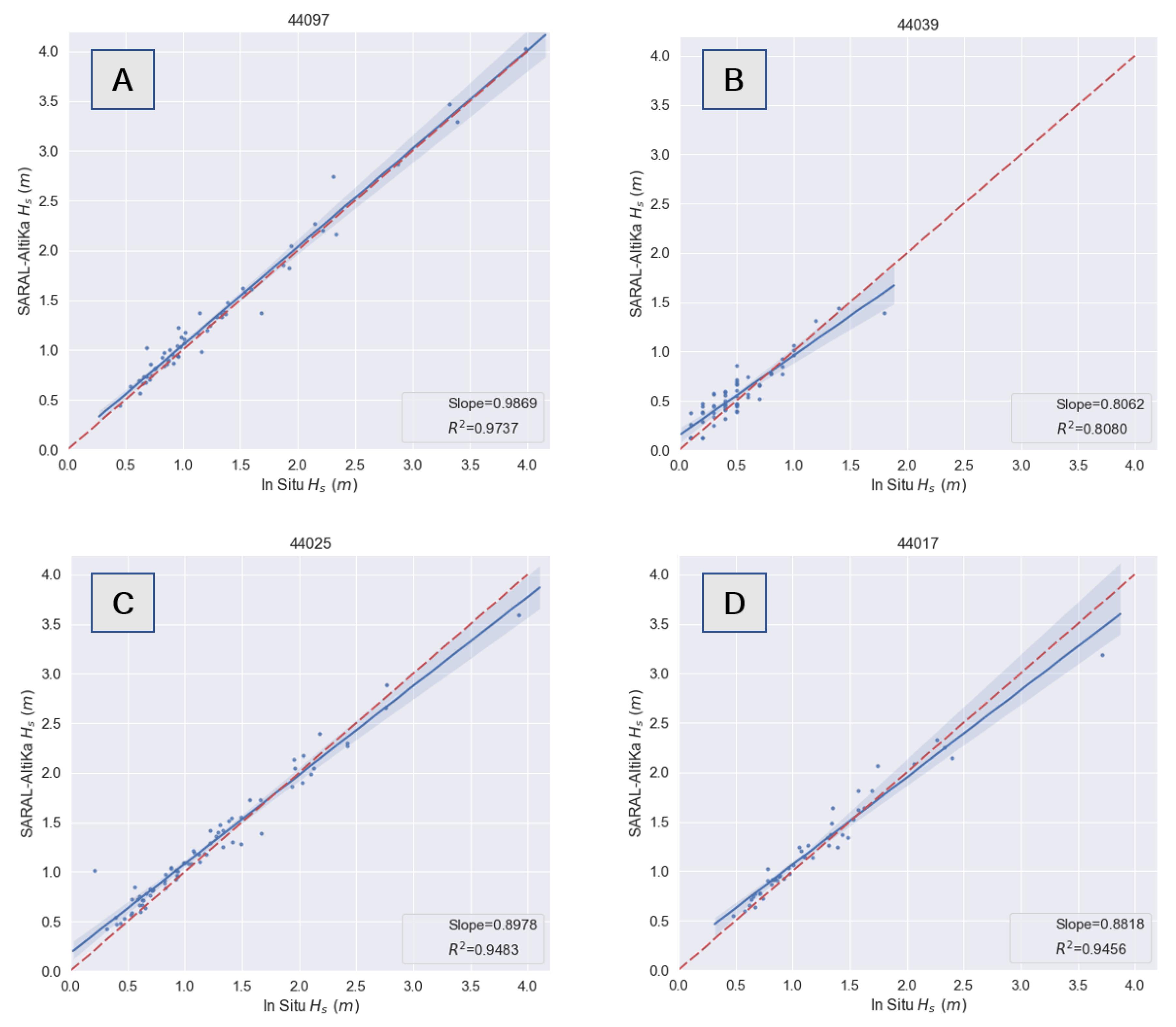
Figure 3 shows the scatter plot comparing measurements with AltiKa’s IGDR and buoy data. In all cases, the regression line closely follows the diagonal line, but there is a tendency to under (over) estimate large (low) values of in most of the reference locations. The slope of the regression lines are less than 1 (zero bias) but more than 0.8, as shown on the bottom right corner on each panel. We refer to it as proportional bias to differentiate from a constant bias in which the regression line is parallel but off to the diagonal. Except for Figure 3B, which is a buoy located within the Long Island Sound, the agreement is within the 99% confidence interval. The high accuracy of for Station 44097, 44025 and 44017—open ocean locations—is consistent with past validation studies [22]. Inaccuracies in the estimation of for sites close to the coast have also been reported [21,22].
Figure 4 shows the scatter plot of the wind speed for in situ and satellite measurements. Compared to , wind speed data show a larger spread (lower ). Figure 4A,C, corresponding to stations located in the open ocean and south of Long Island, shows a proportional bias but the regression line falls around the 99% confidence interval. Figure 4B,D presents stations inside Long Island Sound and near the coast, respectively. In both cases, there is a constant bias with the AltiKa measurements over-predicting the in situ observations. The large constant bias in the BUZM3 tower station is striking and so further analysis was carried out to understand the cause. The time series of the wind speed of this station was compared with Station 95022, which was in operations from 2010 to 2012 (not shown). The two in situ observations are consistent with each other. We thus assume that the bias originates from the altimeter’s calculations, which might not apply for the very shallow coastal area surrounding the BUZM3 station.
Data from Station 44040, which is located on the western side of the Long Island Sound, had too few points, and they are shown in Figure 5 only for completeness. The comparison of AltiKa and in situ observations is shown for: (A) the wind speed ; and (B) the . The station is too close to the coast and only a handful of data points were able to pass the data quality control criteria.
4.2. Time Correlation and RMSE
Consistency is also sought through the calculation of the time correlation of the matched measurements. The correlation for each site is shown in Figure 6. The Pearson correlation for the wind speed is shown in Figure 6A, with correlations equal to or higher than 0.90. Table 2 lists the Pearson correlation coefficient and corresponding p-value, the coefficient of determination and the root mean squared error (RMSE). The figure reveals that the estimation of the wind speed is insensitive to whether the station is located inside or outside of the Long Island Sound. Figure 6B shows the Pearson correlation coefficient for . It shows contrast in correlation values with higher values for locations in the open ocean. Table 3 provides additional performance measures.
Table 2 and Table 3 show the relationship between the altimeter and the buoy for the two variables. The Pearson’s correlations for exceed 0.89. The stations with the lowest correlations (44039, 44040 and BUZM3) are located near the coast. The low correlation and high mean bias of the satellite estimates are attributed to the complex land–sea topographic conditions that surround the station. Not including 44040, the Pearson’s correlation for exceeds 0.91. Another conclusion that can be drawn from the tables is the relatively small RMSE, which is 1.5 m/s or less for , except for BUZM3, and about 15 cm or less for , except for Station 44040. Compared with typical ranges of from 0 to 16 m/s, and of from 0 to 3.5 m, the RMSEs are less than 10% and 5%, respectively. As shown in Figure 3 and Figure 4, these errors can be further reduced by applying systematic error correction methods to the raw data.
4.3. Wind Speed and Relationship Comparison
In this section, a comparison between AltiKa and in situ observations for the relationship between wind speed and significant wave height is assessed. Ocean surface wind speed and wave height are essential variables characterizing the air–sea interaction process of the coupled ocean–atmosphere system. In wave forecasting models, sea surface wind speed and significant wave height have a monotonical relationship under a growing sea until it reaches a fully developed sea. It is at this stage that various relationships have been determined [29]. With AltiKa independently measuring and , it would be apparent that a relationships would be possible. However, this is not the case since the altimeter wind speed measurements are considerably affected by swells, which are not directly coupled with the local wind [30]. The effect of the swells, and in general of the sea state, on the precision and accuracy of surface winds and significant wave heights continues to be an ongoing challenge in remote sensing [31,32]. From the products perspective, long-term statistics show that the proportion of wind waves and swells is geographically dependent with the former generally having more than 80% of the total cases in most areas of the global ocean [33]. The New England’s offshore region, and more generally the northwestern Atlantic, the fraction of the waves that are wind waves is relatively high, especially during the winter season as frequent storms cross over the area [34].
To perform the comparison, a polynomial regression curve is obtained for the two datasets and displayed as the natural logarithm of . We compare the aforementioned relationship between the satellite and buoy measurements for Station 44017, 44025 and 44039 as they have sufficiently large sample size. The buoy wind– regression cannot be computed for Buoy 44097 and Station BUZM3 as they measure only one of the two variables. The relationship for Station 44040 is omitted due to the short sample size, as described above.
Figure 7 compares the sample distributions of in situ and satellite data for and the natural logarithm of . In the two buoy locations, the relationship trend line of the AltiKa data is similar to the trend line of the in situ observations. Table 4 shows the Pearson’s correlations and their respective p-values and root mean squared error (RMSE). The low correlations found reflect the fact that a large fraction of the wave heights are due to swells. Data for Station 44039 show distinct trends but higher correlation. This may be related to the station’s location surrounded by land, which makes the fetch smaller and prevents the influence of swells.
4.4. Validation of the Probability Distribution Function
The validation also compares the underlying Probability Density Function (PDF) of the satellite measurements with in situ observations of and for the period 2014–2019. To have a sufficiently large sample size to determine the PDFs, we increased the sampling radius centered on each station from 0.25 () to 0.5 degrees, denoted as . In this section, three stations, 44017, 44025, and 44039, had a sufficiently large sample to define a distribution with sufficient confidence in both variables. Figure 8 illustrates the main characteristics in these stations. Panels on the left column correspond to distributions of and panels on the right correspond to distributions of . The top row (A and B) shows the empirical PDFs based on in situ observations over the full period. The middle row (C and D) shows the in situ observations that matched in space and in time with the AltiKa measurements. The bottom row (E and F) shows all the AltiKa data points within the sampling radius around the station, which were matched with the in situ observations. Table 5, Table 6 and Table 7 provide more details on the sample size on each case and the parameters of the fitting distributions. Two comparisons are highlighted here. First, in all cases, the distribution of is wider than the distribution of . This happens in the buoy data and consistently in the AltiKa data. Another striking feature in this comparison is that the maximums of the wind distribution of the AltiKa-matched buoy data (C) and the AltiKa data (E) are shifted to lower values of wind compared to all the buoy data (A). Specifically, for the wind in Station 44017, the location of the mode (, where A is the Weibull scale parameter) is 5.78, 5.14 and 5.32 m/s, respectively. This means that the AltiKa systematically misses events with large wind speed values. Comparing the last two numbers we see that the mode of the in situ wind speed (5.14 m/s) is 3.5% smaller than the corresponding mode of the AltiKa data. The shifting of the mode for is not evident when comparing D and F with B in the figure. A second comparison is between the matched in situ observations, C and D, and the matched AltiKa measurements. Here, the corresponding fitting (Weibull distribution) curves of (C and E), and (D and F) match according to the Kolmogorov-Smirnov test given in Table 8 as described below.
Table 5, Table 6 and Table 7 provide the fitting curve parameters for the variables in the three stations analyzed. The tables include the sample sizes of the three datasets to illustrate the small fraction of in situ data that matches the AltiKa data. The in situ data are hourly for Buoys 44017 and 44025 and a higher frequency for Buoy 44039. All three stations had periods of missing data. The sample size of the matched in situ observations is the smallest of the three. In each matched (hour) case, there are about nine data points of Altika passing over , except for Station 44039, where land prevents from collecting data points as in the other stations. The three tables show that is best fit using a Weibull shape, k, equal to 2 and that the scale parameter, A, for the matched data (second and third rows) are similar. In the case of the Weibull’s shape parameter and scale parameters are not similar. To compare how similar are the distributions of the matched cases a two-sample Kolmogorov–Smirnov (KS) test is performed. The results are shown in Table 8. The maximum distance and the p-values are shown in the last two columns of Table 8, respectively. In all cases, except for for Station 44039, the KS statistics are small, indicating that the distributions of the two samples come from the same distribution.
5. Wind Energy Production Estimation
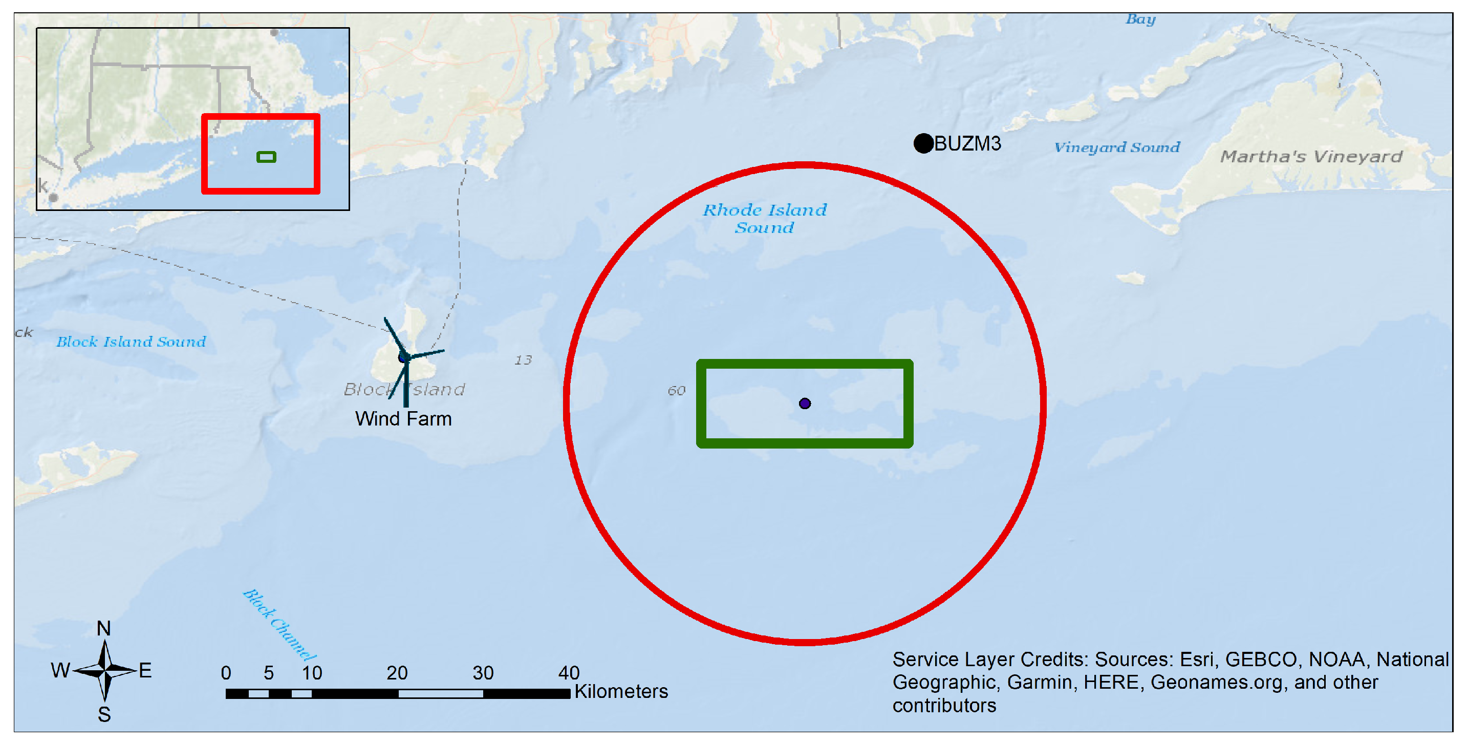
The results described thus far indicate that the AltiKa data point measurements falling within are consistent with the statistics of the reference stations. This is especially true for on stations located in the open ocean. In this section, we estimate the wind resource in the target area between Block Island and Martha’s Vineyard Island shown as a green rectangle in Figure 9. With no direct wind observations in the target area, AltiKa measurements can be used as a first approximation given that they overpass. The AltiKa data, however, must be bias corrected using nearby in situ observations. In addition, to compute the wind power potential, we use the wind power curve of the Block Island’s Wind Farm, which is currently the only wind farm operating in the New England region [35].
The closest wind station is the BUZM3. The AltiKa data passing over this site, however, have a bias, as evident in Figure 4D. The bias is 1.1661 m/s with AltiKa data showing systematically lower values than those from the in situ observations. This bias is corrected to create a new distribution that is combined with the AltiKa data overpassing the target area to create a merged Weibull distribution, as shown in Figure 10. Figure 10A shows the scatter plot and the marginal histograms with fitted Weibull distributions of on the target area and on the BUZM3 station. The merged Weibull distribution is shown in Figure 10B.
Figure 10B shows that the wind density distributions estimated on the BUZM3 station, after bias correction and wind estimated on the target area have slightly different scale parameter, A.
5.1. Wind Energy Density Estimate
The mean energy density, /m, is related to Weibull distribution of the wind observations with scale A and shape k. /m is given by [5]:
where is the Gamma function and is the air density. According to the International Standard Atmosphere (ISA), is set as 1.225 kg/m3 for dry air at 15 °C at sea level.
Using this formula, Table 9 shows the energy density at three locations: the BUZM3, the target location using only AltiKa data and the target location using the merged data.
5.2. Wind Power Generation Estimate
Wind power generation depends on the design of the wind turbine and the wind flowing across its axis plane. Every wind turbine has a characteristic power performance curve that relates the energy production to the hub-height wind speed. The (power) curves summarize the technical details of the wind turbine’s components such as wind turbine rotors and electrical generators [36], and are normally provided by the manufacturer. Due to its proximity to the target area—the green box in Figure 9—in this study, the power curve of the wind farm located at the Block Island site is used. The parameters in this curve were the hub-height (100 m), the rated power (16 MW) and the cut in and cut off wind speeds of 2.1 and 26.1 m/s, respectively. The 10-m wind distribution obtained in the previous section is extrapolated to 100 m using the recommended Power Law vertical wind shear model [37]. Furthermore, experience with the time series of power generation and corresponding wind speeds of the wind farm indicates that the power curve can be modeled using the wind distribution quantiles [38], as shown in Equation (3).
where P is power output (MW), is the maximum power output of the power plant, w is wind speed (m/s) at the hub level, and are wind speed at and of turbine rated power and and are cut-in and cut-off wind speed, respectively. While most of the parameters from the reference (Block Island) wind farm were used, the rated power is not because it is intrinsic to the farm design. To eliminate the difference between the reference rated power and that from the hypothetical wind farm, the wind power is normalized, given by:
where is the normalized wind power, P is power output (MW) and and are minimum and maximum power output. After normalization, the wind power is shown in Figure 11. While the estimated wind capacity is generally provided as an annual average, the data allow for assessing the variation of power capacity per hour of the day and per season. This is shown in Figure 12.
In Figure 12A, it is evident that during summer and to a lesser extent during spring and autumn, a diurnal cycle is observed. In the summer, stronger winds are found at 19 UTC (16:00 local time). In Figure 12B, the average power output capacity values appear off by 3 h. It is evident that, in both the merged power (12A) and the AltiKa-alone (12B) data, winds are stronger in winter than in the summer.
Since the SARAL/AltiKa ground track passes over our region of interest only around 10 and 23 UTC, the data miss the diurnal cycle. To compute this bias, we calculate the multi-year average of buoy data per hour to assess the amplitude of the diurnal cycle of the wind for two representative stations. One station is close to the coast (BUZM3) and the other (44017) is about 40 km away from the nearest coast. The averages are displayed in Figure 13, which shows that the amplitudes are about 1 m/s in summer and in winter. These amplitudes are small compared to the seasonal variation, indicated by the distance between the summer and winter lines. The amplitude of the diurnal variation of the (not shown) for Station 44017 is less than 2 cm.
Figure 13 shows that the amplitude of the wind speed diurnal cycle is stronger during the summer months, especially in stations near the coast. This is consistent with the expected land–sea breeze mechanism resulted from the unequal heating rates of land and water.
6. Conclusions
This study evaluated the SARAL/AltiKa data for their use on offshore wind resource assessments and their potential use in wind and wave characterization in the region off the coast of southern New England states. The SARAL/AltiKa dataset was selected in this study for its improved footprint resolution to capture the mesoscale characteristics of water and air characteristics, especially near the coastal areas. While satellite altimetry is already a mature technology for open seas, its full potential for coastal studies remains largely unexploited. A major challenge besides the sensor’s increased sensibility to water vapor is the small sample size available to produce statistics with reduced noise needed for energy assessment on a target site. We addressed this problem by collecting samples within geographical domains around the reference sites larger than the satellite footprint. We determined a trade-off radius that increased the sample size at the expense of systematic error increment. In addition, to reduce noise, we computed hourly and overpass averages. Our analysis demonstrated that both procedures did not impact the calculations of wind energy resources.
Specifically, our results corroborates the high degree of accuracy of the AltiKa data compared with in situ observations with correlations exceeding 0.91 correlations for and above 0.97 for in open ocean sites. For coastal sites, two types of bias were evident: the mean bias and the proportional bias. The mean bias was evident for the wind data in coastal sites (Figure 5B,D), whereas the proportional bias was more evident for in the coastal site (Figure 5B) and to less extent in open ocean sites (Figure 5C,D).
The evaluation of the AltiKa data included assessing the relationship of simultaneous measurements of wind speed and . The empirical relationship between them has been used for ship safety, offshore structure designs and offshore operations. We compared this relationship with that from sites that provided both variables. This study shows that the relationship was reproduced in open ocean buoys (Figure 7A,B), but it showed large differences for the coastal site (Figure 7C) studied. The validation of the full distribution of winds required additional treatment and the sample size was barely enough to fit an appropriate curve considering the short sample size. Our results indicate that the Weibull distribution fits well the histograms of satellite wind speed and , and that the parameters for corresponding histograms from the in situ observations were very similar. In general, the SARAL/AltiKa data performed very well except for near the coast and inside the Long Island Sound. This is consistent with previous studies [17,39] carried out in other locations.
The results left unanswered how the land–sea breeze and in general the diurnal cycle is represented in the AltiKa data as the distance from the coastal boundary increases. The results do show that progress is needed to further improve the representation of winds and waves closer to the coast and on approaches to reduce land data contamination. This study could be extended to respond to questions related to offshore marine logistics and monitoring. For instance, we would like to know how these measurements relate to or can be combined with measurements from other satellite data missions to reduce the time gap between overpasses to be able to perform sensible time interpolations. The integration of these datasets, especially those distributed in real-time, into a coastal observing system should have a tremendous impact for the metocean monitoring and offshore energy engineering applications.
Author Contributions
Conceptualization, M.P. and P.M.; methodology, M.P. and X.L.; software, X.L. and P.M.; validation, X.L., P.M. and Y.Y.; formal analysis, M.P. and P.M.; investigation, X.L., Y.Y. and P.M.; resources, X.L. and P.M.; data curation, X.L., P.M. and Y.Y.; writing—original draft preparation, M.P.; writing—review and editing, X.L.; visualization, X.L.; supervision, M.P.; project administration, M.P.; and funding acquisition, M.P. All authors have read and agreed to the published version of the manuscript.
Funding
This research was funded by the Eversource Energy Center, grant number AG200208.
Acknowledgments
We acknowledge the comments given by four anonymous reviewers, which greatly improved the content and clarity of the manuscript.
Conflicts of Interest
The authors declare no conflict of interest.
Abbreviations
The following abbreviations are used in this manuscript:
| SWH | Significant Wave Height |
| RMSE | Root Mean Squared Error |
| OGDR | Operational Geophysical Data Record |
| IGDR | Interim Geophysical Data Records |
| GDR | Geophysical Data Records |
| SSH | Sea Surface Height |
| Sample Collecting radius | |
| 0.5 Degrees Collecting radius | |
| Significant Wave Height | |
| Wind Speed at 10 m |
References
- Coastline County Population Continues to Grow. Available online: https://www.census.gov/library/stories/2018/08/coastal-county-population-rises.html (accessed on 10 June 2020).
- Mills, A.D.; Millstein, D.; Jeong, S.; Lavin, L.; Wiser, R.; Bolinger, M. Estimating the Value of Offshore Wind along the United States’ Eastern Coast. Environ. Res. Lett. 2018, 13, 094013. [Google Scholar] [CrossRef]
- Massachusetts Activities. Available online: https://www.boem.gov/renewable-energy/state-activities/massachusetts-activities (accessed on 24 June 2020).
- Eurek, K.; Sullivan, P.; Gleason, M.; Hettinger, D.; Heimiller, D.; Lopez, A. An Improved Global Wind Resource Estimate for Integrated Assessment Models. Elsevier 2017, 64, 552–567. [Google Scholar] [CrossRef]
- Ahsbahs, T.; MacLaurin, G.; Draxl, C.; Jackson, C. US East Coast Synthetic Aperture Radar Wind Atlas for Offshore Wind Energy. Wind. Energy Sci. 2020. [Google Scholar] [CrossRef]
- Grilli, A.R.; Spaulding, M.L. Offshore Wind Resource Assessment in Rhode Island Waters. Sage J. 2013, 37, 579–594. [Google Scholar] [CrossRef]
- Exertier, P.; Bonnefond, P.; Nicolas, J.; Barlier, F. Contributions of Satellite Laser Ranging to Past and Future Radar Altimetry Missions. Surv. Geophys. 2001, 22, 491–507. [Google Scholar] [CrossRef]
- Ribal, A.; Young, I.R. 33 Years of Globally Calibrated Wave Height and Wind Speed Data Based on Altimeter Observations. Sci. Data 2019, 6, 77. [Google Scholar] [CrossRef] [Green Version]
- Bronner, E.; Guillot, A.; Picot, N.; Noubel, J. Saral/AltiKa Products Handbook. Available online: https://www.mosdac.gov.in/data/Missions/saral/resource/SALP-MU-M-OP-15984-CN_0102[1]_handbook.pdf (accessed on 24 November 2018).
- Cavaleri, L.; Abdalla, S.; Benetazzo, A.; Bertotti, L.; Bidlot, J.; Breivik, O.; Carniel, S.; Jensen, R.E.; Portilla-Yandun, J.; Rogers, W.E.; et al. Wave Modelling in Coastal and Inner Seas. Prog. Oceanogr. 2018. [Google Scholar] [CrossRef]
- Wind to Wave Relationship Reference. Available online: www.weather.gov/media/akq/marine/Wind_Wave_Relationship_Reference.pdf (accessed on 15 December 2019).
- Pandey, P.C.; Gairola, R.M.; Gohil, B.S. Wind-Wave Relationship from SEASAT Radar Altimeter Data. Bound. Layer Meteorol. 1986, 37, 263–269. [Google Scholar] [CrossRef]
- O’Donnell, J.; Wilson, R.E.; Lwiza, K.; Whitney, M.; Bohlen, W.F.; Codiga, D.; Fribance, D.B.; Fake, T.; Bowman, M.; Varekamp, J. The Physical Oceanography of Long Island Sound. In Long Island Sound: Prospects for the Urban Sea; Latimer, J.S., Tedesco, M.A., Swanson, R.L., Yarish, C., Stacey, P.E., Garza, C., Eds.; Springer: New York, NY, USA, 2014; pp. 79–158. ISBN 978-1-4614-6125-8. [Google Scholar]
- Grilli, A.R.; Spaulding, M.L.; Crosby, A.; Sharma, R. Evaluation of Wind Statistics and Energy Resources in Southern RI Coastal Waters. Chapter 20 of Technical Report, Rhode Island Ocean Special Area Management Plan: Ocean SAMP-Volume 2, 2010. Available online: https://tethys.pnnl.gov/publications/rhode-island-ocean-special-area-management-plan-ocean-samp-volume-2 (accessed on 20 December 2020).
- Andreas, E.L.; Mahrt, L.; Vickers, D. A New Drag Relation for Aerodynamically Rough Flow over the Ocean. J. Atmos. Sci. 2012, 69, 2520–2537. [Google Scholar] [CrossRef]
- Verron, J.; Sengenes, P.; Lambin, J.; Noubel, J.; Steunou, N.; Guillot, A.; Picot, N.; Coutin-Faye, S.; Sharma, R.; Gairola, R.M.; et al. The SARAL/AltiKa Altimetry Satellite Mission. Taylor Fr. 2015, 38, 2–21. [Google Scholar] [CrossRef]
- Sepulveda, H.H.; Queffeulou, P.; Ardhuin, F. Assessment of SARAL/AltiKa Wave Height Measurements Relative to Buoy, Jason-2, and Cryosat-2 Data. Taylor Fr. 2015, 38, 449–465. [Google Scholar] [CrossRef] [Green Version]
- Saral (Satellite with ARgos and ALtiKa). Available online: https://earth.esa.int/web/eoportal/satellite-missions/s/saral (accessed on 4 June 2019).
- Gerald, D.; Lamy, A.; Pujol, I.; Jettou, G. The Drifting Phase of SARAL: Securing Stable Ocean Mesoscale Sampling with an Unmaintained Decaying Altitude. Remote Sens. 2018, 10, 1051. [Google Scholar] [CrossRef] [Green Version]
- Lillibridge, J.; Scharroo, R.; Abdalla, S.; Vandemark, D. One- and Two-Dimensional Wind Speed Models for Ka-Band Altimetry. J. Atmos. Oceanic Technol. 2014, 31, 630–638. [Google Scholar] [CrossRef]
- Verron, J.; Bonnefond, P.; Aouf, L.; Birol, F.; Bhowmick, S.; Calmant, S.; Conchy, T.; Crétaux, J.-F.; Dibarboure, G.; Dubey, A.; et al. The Benefits of the Ka-Band as Evidenced from the SARAL/AltiKa Altimetric Mission: Scientific Applications. Remote Sens. 2018, 10, 163. [Google Scholar] [CrossRef] [Green Version]
- Bonnefond, P.; Verron, J.; Aublanc, J.; Babu, K.N.; Bergé-Nguyen, M.; Cancet, M.; Chaudhary, A.; Crétaux, J.-F.; Frappart, F.; Haines, B.J.; et al. The Benefits of the Ka-Band as Evidenced from the SARAL/AltiKa Altimetric Mission: Quality Assessment and Unique Characteristics of AltiKa Data. Remote Sens. 2018, 10, 83. [Google Scholar] [CrossRef] [Green Version]
- Chelton, D.B.; Ries, J.C.; Haines, B.J.; Fu, L.-L.; Callahan, P.S. Satellite Altimetry. In Satellite Altimetry and Earth Sciences: A Handbook of Techniques and Applications; Fu, L.-L., Cazenave, A., Eds.; Academic Press: San Diego, CA, USA, 2001; pp. 1–131. [Google Scholar]
- Prandi, P.; Philipps, S.; Pignot, V.; Picot, N. SARAL/AltiKa Global Statistical Assessment and Cross-Calibration with Jason-2. Taylor Fr. 2015, 38, 297–312. [Google Scholar] [CrossRef]
- Zieger, S.; Vinoth, J.; Young, I.R. Joint Calibration of Multiplatform Altimeter Measurements of Wind Speed and Wave Height over the Past 20 Years. J. Atmos. Ocean. Technol. 2009, 26, 2549–2564. [Google Scholar] [CrossRef]
- Martíenez, À.; del Ríeo, F.J.; Riu, J.; Rius, F.X. Detecting Proportional and Constant Bias in Method Comparison Studies by Using Linear Regression with Errors in Both Axes. Chemom. Intell. Lab. 1999, 49, 179–193. [Google Scholar] [CrossRef]
- Observation Data Descriptions. Available online: https://www.ndbc.noaa.gov/obsdes.shtml (accessed on 13 December 2020).
- Do NDBC’s Meteorological and Oceanographic Sensors Measure Data for the Entire Hour? Available online: https://www.ndbc.noaa.gov/acq.shtml (accessed on 7 August 2020).
- Pierson, W.J. Comment on “Effects of Sea Maturity on Satellite Altimeter Measurements” by Roman E. Glazman and Stuart H. Pilorz. J. Geophys. Res. Ocean. 1991, 96, 4973–4977. [Google Scholar] [CrossRef] [Green Version]
- Gourrion, J.; Vandemark, D.; Bailey, S.; Chapron, B. Satellite altimeter models for surface wind speed developed using ocean satellite crossovers. IFREMER Tech. Rep. DROOS-2000-02, p. 62. Available online: https://topex.wff.nasa.gov/wp-content/uploads/ifremer.droos_.2000-02.pdf (accessed on 22 December 2020).
- Abdalla, S. Active Techniques for wind and wave observations: Radar altimeter. In Proceedings of the Seminar on Use of Satellite Observations in Numerical Weather Prediction, Reading, UK, 8–12 September 2014. [Google Scholar]
- Reale, F.; Dentale, F.; Carratelli, E.P.; Fenoglio-Marc, L. Influence of Sea State on Sea Surface Height Oscillation from Doppler Altimeter Measurements in the North Sea. Remote Sens. 2018, 10, 1100. [Google Scholar] [CrossRef] [Green Version]
- Chen, G.; Chapron, B.; Ezraty, R.; Vandemark, D. A global view of swell and wind sea climate in the ocean by satellite altimeter and scatterometer. J. Atmos. Oceanic Tech. 2002, 19, 1849–1859. [Google Scholar] [CrossRef]
- Colle, B.A.; Sienkiewicz, M.J.; Archer, C.; Veron, D.; Veron, F.; Kempton, W.; Mak, J.E. Improving the mapping and prediction of offshore wind resources (IMPOWR): Experimental overview and first results. Bull. Am. Meteorol. Soc. 2016, 97, 1377–1390. [Google Scholar] [CrossRef]
- Musial, W.; Beiter, P.; Schwabe, P.; Tian, T.; Stehly, T.; Spitsen, P.; Robertson, A.; Gevorgian, V. 2016 Offshore Wind Technologies Market Report; NREL/TP-5000-68587; DOE/GO-102017-5031; National Renewable Energy Lab.: Golden, CO, USA, 2017. [Google Scholar] [CrossRef]
- Manwell, J.F.; McGowan, J.G.; Rogers, A.L. Wind Energy Explained: Theory, Design and Application, 2nd ed.; John Wiley & Sons: Hoboken, NJ, USA, 2010; 705p. [Google Scholar]
- Metocean Characterization Recommended Practices for U.S. Offshore Wind Energy. Available online: https://tethys.pnnl.gov/publications/metocean-characterization-recommended-practices-us-offshore-wind-energy (accessed on 5 July 2020).
- Mur Amada, J.; Comech Moreno, M.P. Reactive Power Injection Strategies For Wind Energy Regarding Its Statistical Nature. In Proceedings of the 6th International Workshop on Large-Scale Integration of Wind Power and Transmission Networks for Offshore Wind Farms, Delft, The Netherlands, 26–28 October 2006. [Google Scholar]
- Kumar, U.M.; Swain, D.; Sasamal, S.K.; Reddy, N.N.; Ramanjappa, T. Validation of SARAL/AltiKa Significant Wave Height and Wind Speed Observations over the North Indian Ocean. J. Atmos. Sol. Terr. Phys. 2015, 135, 174–180. [Google Scholar] [CrossRef]
Figure 1.
Locations of buoy sensors measuring wind speed and , as well as the BUZM3 wind tower station. Data are displayed in a coordinate system in which units are in degrees, and where degrees are represented as equally spaced over the x and y scale. The red bound and green bound represent 0.25 and 0.5 decimal degree radii from a buoy. Buoys are displayed either as a circle or triangle to show whether they are within or outside of 50 km from land, respectively.

Figure 2.
Pass averaged SARAL/AltiKa sample size and proportional bias around Buoy 44025. The red box highlights .
Figure 2.
Pass averaged SARAL/AltiKa sample size and proportional bias around Buoy 44025. The red box highlights .

Figure 3.
Comparison of significant wave height, , between SARAL/AltiKa and selected buoys at stations 44097 (A), 44039 (B), 44025 (C), and 44017 (D). Matched measurements denoted as blue dots are those falling within radius . In each case, the fitting linear regression line is shown as a continuous blue line with their corresponding 99% confidence interval in shaded blue.

Figure 4.
Comparison of 10-meter wind speed, , between SARAL/AltiKa and selected buoys at stations 44025 (A), 44039 (B), 44017 (C), and BUZM3 (D). Matched measurements denoted as blue dots are those falling within radius . In each case, the fitting linear regression line is shown as a continuous blue line with their corresponding 99% confidence interval in shaded blue.

Figure 5.
Comparison of (A) and (B) between SARAL/AltiKa and buoy station 44040. Matched measurements denoted as blue dots are those falling within radius . The fitting linear regression line is shown as a continuous blue line with their corresponding 99% confidence interval in shaded blue. In this case, the sample size is too small. The large discrepancy of the regression line with respect to the diagonal is mostly attributed to land data contamination.

Figure 6.
Pearson correlations between SARAL/AltiKa measurements and in situ observations for: (A) ; and (B) . The circles denote the collecting sample area with radius .
Figure 6.
Pearson correlations between SARAL/AltiKa measurements and in situ observations for: (A) ; and (B) . The circles denote the collecting sample area with radius .

Figure 7.
Comparison between satellite wind speed and data within of buoy (A) 44017 and (B) 44025 and 10 km of buoy (C) 44039.
Figure 7.
Comparison between satellite wind speed and data within of buoy (A) 44017 and (B) 44025 and 10 km of buoy (C) 44039.

Figure 8.
Probability density functions of (left) and (right) for Buoy 44017 for the period 2014–2019: (A,B) PDFs based on all the in situ data available for the period; (C,D) PDFs for the space and time matched cases of in situ observations; and (E,F) PDFs for all the matched AltiKa measurements. The fitting Weibull distribution curves defined in Table 5 are also shown.

Figure 9.
Map of locations of BUZM3 station, wind farm and target area (green rectangle). The red circle represents of the center of the target area.
Figure 9.
Map of locations of BUZM3 station, wind farm and target area (green rectangle). The red circle represents of the center of the target area.

Figure 10.
(A) The scatter plot and the marginal histograms with fitted Weibull distributions of the from target area SARAL/AltiKa and BUZM3 station. A and k are Weibull parameters of scale and shape. (B) The Weibull distribution (red line) showing the wind characteristics in the target area estimated from target area SARAL/AltiKa (gray line) and BUZM3 station (dashed black line). Points A and B are mean () from observations of BUZM3 station and target area SARAL/AltiKa, respectively.

Figure 11.
Wind power curve at the target area based on wind data from nearby wind farm. A and B are cut-in wind speed and cut-off wind speed, respectively.
Figure 11.
Wind power curve at the target area based on wind data from nearby wind farm. A and B are cut-in wind speed and cut-off wind speed, respectively.

Figure 12.
Seasonality and diurnal characteristics of power output capacity in percent. Power output capacity are averaged by month and hour. (A) Merged data. Approximate observations per cell: 500. (B) Target area SARAL/AltiKa. Approximate observations per cell: 10.
Figure 12.
Seasonality and diurnal characteristics of power output capacity in percent. Power output capacity are averaged by month and hour. (A) Merged data. Approximate observations per cell: 500. (B) Target area SARAL/AltiKa. Approximate observations per cell: 10.

Figure 13.
(Top) BUZM3 Station and (Bottom) Buoy 44017 diurnal variability; 1999–2019 average with 95% confidence intervals.
Figure 13.
(Top) BUZM3 Station and (Bottom) Buoy 44017 diurnal variability; 1999–2019 average with 95% confidence intervals.


Table 1.
In situ observation sites used in this study.
| Station Number | Station Name | Anemometer Height (m) | Wind Speed | Significant Wave Height |
|---|---|---|---|---|
| 44025 | Long Island | 4.1 | 🗸 | 🗸 |
| 44039 | Central Long Island | 3.5 | 🗸 | 🗸 |
| 44040 | Western Long Island | 3.5 | 🗸 | 🗸 |
| 44097 | Block Island | N/A | 🗸 | |
| 44017 | Montauk Point | 4.1 | 🗸 | 🗸 |
| BUZM3 | Buzzards Bay | 24.8 | 🗸 |
Table 2.
Correlation r, coefficient of determination and Root Mean Square Errors (RMSE) between in situ and SARAL/AltiKa measurements for the matched cases.
Table 2.
Correlation r, coefficient of determination and Root Mean Square Errors (RMSE) between in situ and SARAL/AltiKa measurements for the matched cases.
| Buoy | Pearson’s r (p-Value) | RMSE | |
|---|---|---|---|
| 44025 | 0.9290 (<0.01) | 0.8596 | 1.3544 |
| 44039 | 0.9220 (<0.01) | 0.8080 | 1.0730 |
| 44017 | 0.9430 (<0.01) | 0.8737 | 1.0470 |
| BUZM3 | 0.8985 (<0.01) | 0.6579 | 1.8289 |
| 44040 | 0.9199 (0.02) | 0.4152 | 1.5039 |
Table 3.
Correlation, coefficient of determination and Root Mean Square Errors (RMSE) between in situ and SARAL/AltiKa measurements for the matched cases.
Table 3.
Correlation, coefficient of determination and Root Mean Square Errors (RMSE) between in situ and SARAL/AltiKa measurements for the matched cases.
| Buoy | Pearson’s r (p-Value) | RMSE | |
|---|---|---|---|
| 44097 | 0.9886 (<0.01) | 0.9737 | 0.1199 |
| 44039 | 0.9147 (<0.01) | 0.8080 | 0.1405 |
| 44025 | 0.9802 (<0.01) | 0.9483 | 0.1540 |
| 44017 | 0.9780 (<0.01) | 0.9456 | 0.1383 |
| 44040 | 0.6671 (0.22) | −5.4088 | 0.6301 |
Table 4.
Satellite and corresponding buoy Pearson correlation and RSME values between wind speed and .
Table 4.
Satellite and corresponding buoy Pearson correlation and RSME values between wind speed and .
| Area of Interest | SARAL-AltiKa | Corresponding Buoy | ||||
|---|---|---|---|---|---|---|
| Pearson’s r (p-Value) | RMSE | Slope | Pearson’s r (p-Value) | RMSE | Slope | |
| 44017 | 0.6965 (<0.01) | 6.8952 | 0.0962 | 0.6888 (<0.01) | 6.9398 | 0.0995 |
| 44025 | 0.6995 (<0.01) | 7.5429 | 0.1058 | 0.7334 (<0.01) | 7.0424 | 0.1132 |
| 44039 | 0.8052 (<0.01) | 7.1181 | 0.1652 | 0.7853 (<0.01) | 6.8956 | 0.2129 |
Table 5.
Weibull shape and scale values with 95% confidence interval in parentheses for satellite and buoy data around Buoy 44017.
Table 5.
Weibull shape and scale values with 95% confidence interval in parentheses for satellite and buoy data around Buoy 44017.
| Buoy 44017 | Sample Size | Wind Speed (CI) | (CI) | ||
|---|---|---|---|---|---|
| Weibull Scale (A) | Weibull Shape (k) | Weibull Scale (A) | Weibull Shape (k) | ||
| Full Buoy data | 31,351 | 8.19 (8.14, 8.23) | 2 | 1.49 (1.48, 1.50) | 1.88 (1.86, 1.89) |
| IGDR-corresponding Buoy data | 134 | 7.27 (6.68, 7.91) | 2 | 1.39 (1.28, 1.51) | 2.14 (1.90, 2.40) |
| IGDR data | 1221 | 7.52 (7.32, 7.34) | 2 | 1.54 (1.50, 1.58) | 2.16 (2.07, 2.25) |
Table 6.
Weibull shape and scale values with 95% confidence interval in parentheses for satellite and buoy data around Buoy 44025.
Table 6.
Weibull shape and scale values with 95% confidence interval in parentheses for satellite and buoy data around Buoy 44025.
| Buoy 44025 | Sample Size | Wind Speed (CI) | (CI) | ||
|---|---|---|---|---|---|
| Weibull Scale (A) | Weibull Shape (k) | Weibull Scale (A) | Weibull Shape (k) | ||
| Full Buoy data | 42399 | 8.22 (8.18, 8.26) | 2 | 1.46 (1.45, 1.47) | 1.89 (1.88, 1.90) |
| IGDR-corresponding Buoy data | 195 | 7.62 (7.10, 8.18) | 2 | 1.34 (1.24, 1.45) | 1.86 (1.68, 2.07) |
| IGDR data | 1117 | 7.02 (6.82, 7.23) | 2 | 1.33 (1.29, 1.38) | 1.98 (1.90, 2.07) |
Table 7.
Weibull shape and scale values with 95% confidence interval in parentheses for satellite and buoy data around Buoy 44039.
Table 7.
Weibull shape and scale values with 95% confidence interval in parentheses for satellite and buoy data around Buoy 44039.
| Buoy 44039 | Sample Size | Wind Speed (CI) | (CI) | ||
|---|---|---|---|---|---|
| Weibull Scale (A) | Weibull Shape (k) | Weibull Scale (A) | Weibull Shape (k) | ||
| Full Buoy data | 231577 | 6.52 (6.51, 6.53) | 2 | 0.51 (0.51, 0.51) | 1.38 (1.37, 1.38) |
| IGDR-corresponding Buoy data | 129 | 6.36 (5.83, 6.94) | 2 | 0.54 (0.48, 0.60) | 1.69 (1.49, 1.92) |
| IGDR data | 355 | 6.48 (6.15, 6.82) | 2 | 0.95 (0.88, 1.01) | 1.65 (1.53, 1.78) |
Table 8.
Two sample Kolmogorov–Smirnov test results between IGDR-corresponding buoy data and IGDR data.
Table 8.
Two sample Kolmogorov–Smirnov test results between IGDR-corresponding buoy data and IGDR data.
| Buoy | Sample Size | K-S Value (p-Value) | K-S Value (p-Value) | |
|---|---|---|---|---|
| IGDR-Corresponding Buoy Data | IGDR Data | |||
| 44017 | 134 | 1221 | 0.0793 (0.42) | 0.1154 (0.07) |
| 44025 | 195 | 1117 | 0.1239 (0.01) | 0.0809 (0.22) |
| 44039 | 128 | 335 | 0.1055 (0.23) | 0.3435 (<0.01) |
Table 9.
Comparison on the Mean Energy Density (E), the Weibull parameters and the wind energy parameters at the BUZM3, at the target location using only AltiKa data and the target location using the merged data. and are the most frequent and of the maximum wind energy carrier, respectively.
Table 9.
Comparison on the Mean Energy Density (E), the Weibull parameters and the wind energy parameters at the BUZM3, at the target location using only AltiKa data and the target location using the merged data. and are the most frequent and of the maximum wind energy carrier, respectively.
| Data | E | A | k | |||
|---|---|---|---|---|---|---|
| BUZM3 station | 362 | 7.63 | 2 | 6.75 | 5.39 | 10.77 |
| Target area SARAL/AltiKa | 466 | 8.3 | 2 | 7.59 | 6.06 | 12.11 |
| Merged data | 401 | 7.9 | 2 | 7.17 | 5.72 | 11.44 |
Publisher’s Note: MDPI stays neutral with regard to jurisdictional claims in published maps and institutional affiliations. |
© 2020 by the authors. Licensee MDPI, Basel, Switzerland. This article is an open access article distributed under the terms and conditions of the Creative Commons Attribution (CC BY) license (http://creativecommons.org/licenses/by/4.0/).
Share and Cite
MDPI and ACS Style
Li, X.; Mitsopoulos, P.; Yin, Y.; Peña, M. SARAL-AltiKa Wind and Significant Wave Height for Offshore Wind Energy Applications in the New England Region. Remote Sens. 2021, 13, 57. https://0-doi-org.brum.beds.ac.uk/10.3390/rs13010057
AMA Style
Li X, Mitsopoulos P, Yin Y, Peña M. SARAL-AltiKa Wind and Significant Wave Height for Offshore Wind Energy Applications in the New England Region. Remote Sensing. 2021; 13(1):57. https://0-doi-org.brum.beds.ac.uk/10.3390/rs13010057
Chicago/Turabian StyleLi, Xinba, Panagiotis Mitsopoulos, Yue Yin, and Malaquias Peña. 2021. "SARAL-AltiKa Wind and Significant Wave Height for Offshore Wind Energy Applications in the New England Region" Remote Sensing 13, no. 1: 57. https://0-doi-org.brum.beds.ac.uk/10.3390/rs13010057
Note that from the first issue of 2016, this journal uses article numbers instead of page numbers. See further details here.