Structure-from-Motion-Derived Digital Surface Models from Historical Aerial Photographs: A New 3D Application for Coastal Dune Monitoring


 and
and
Abstract
:
1. Introduction
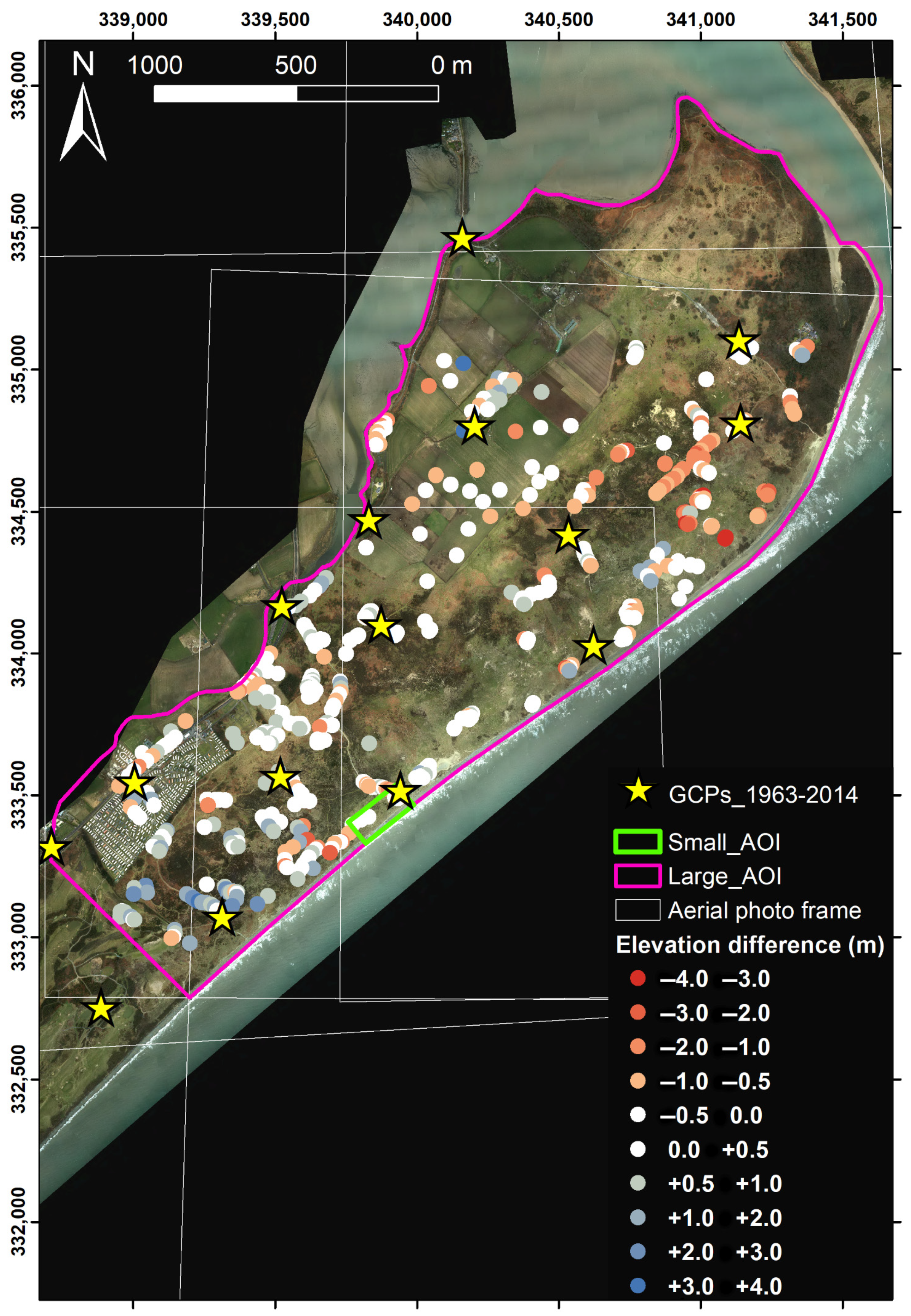
2. Study Area
3. Materials and Methods
3.1. Historical Aerial Photographic Dataset
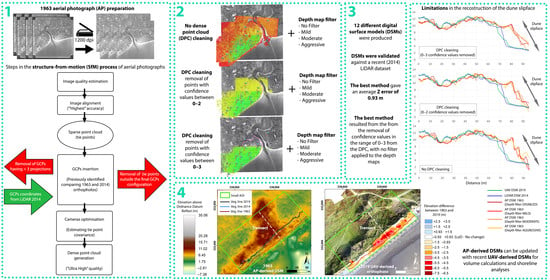
3.1.1. SfM Processing of Historical Aerial Photographs
3.2. LiDAR Dataset
3.3. UAV Dataset
SfM Processing of UAV Images
3.4. 1963 DSM Accuracy Assessment and Validation
3.5. Geomorphic Changes and Volumetric Variation
4. Results
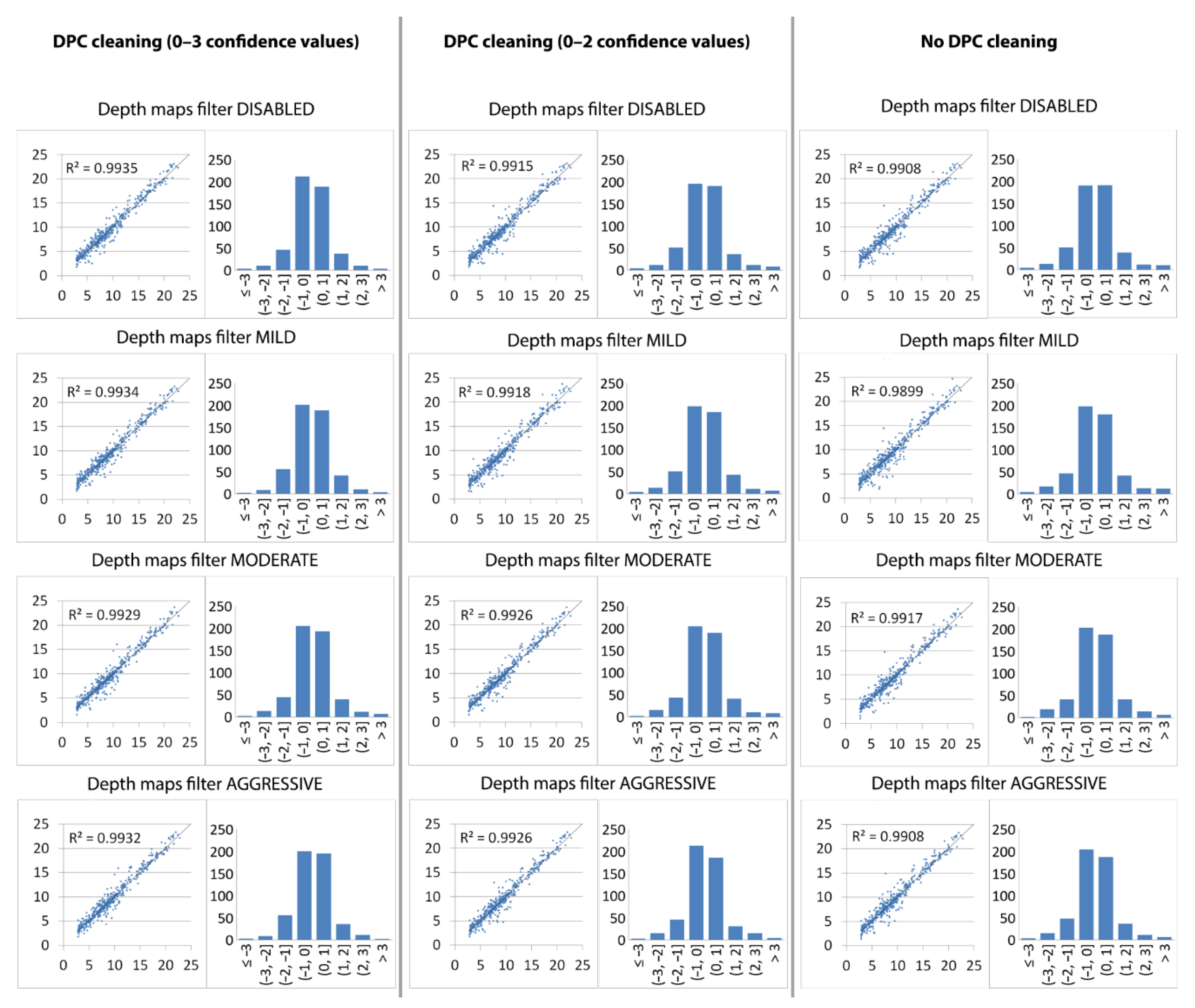
4.1. Accuracy Assessment of Aerial-Photograph-Derived DSMs
4.2. Geomorphic Changes and Volumetric Variation
5. Discussion and Conclusions
Author Contributions
Funding
Informed Consent Statement
Data Availability Statement
Acknowledgments
Conflicts of Interest
Abbreviations
| AOI | Area of Interest |
| AP | Aerial Photograph |
| DEM | Digital Elevation Model |
| DoD | DEM of Difference |
| DPC | Dense Point Cloud |
| DSM | Digital Surface Model |
| GCP | Ground Control Point |
| DGNSS | Differential Global Navigation Satellite System |
| LiDAR | Light Detection And Ranging |
| LoD | Limit of Detection |
| MAE | Mean Absolute Error |
| OSNI | Ordnance Survey of Northern Ireland |
| RMSE | Root Mean Square Error |
| SDE | Standard Deviation Error |
| SfM | Structure-from-Motion |
| SPC | Sparse Point Cloud |
| UAV | Unmanned Aerial Vehicle |
References
- Guisado-Pintado, E.; Jackson, D.W.T.; Rogers, D. 3D mapping efficacy of a drone and terrestrial laser scanner over a temperate beach-dune zone. Geomorphology 2019, 328, 157–172. [Google Scholar] [CrossRef]
- Fonstad, M.A.; Dietrich, J.T.; Courville, B.C.; Jensen, J.L.; Carbonneau, P.E. Topographic structure from motion: A new development in photogrammetric measurement. Earth Surf. Proc. Land. 2013, 38, 421–430. [Google Scholar] [CrossRef] [Green Version]
- Splinter, K.D.; Harley, M.D.; Turner, I.L. Remote Sensing Is Changing Our View of the Coast: Insights from 40 Years of Monitoring at Narrabeen-Collaroy, Australia. Remote Sens. 2018, 10, 1744. [Google Scholar] [CrossRef] [Green Version]
- Montaño, J.; Coco, G.; Antolínez, J.A.; Beuzen, T.; Bryan, K.R.; Cagigal, L.; Castelle, B.; Davidson, M.A.; Goldstein, E.B.; Ibaceta, R.; et al. Blind testing of shoreline evolution models. Sci. Rep. 2020, 10, 2137. [Google Scholar] [CrossRef] [PubMed] [Green Version]
- Vitousek, S.; Barnard, P.L.; Limber, P.; Erikson, L.; Cole, B. A model integrating longshore and cross-shore processes for predicting long-term shoreline response to climate change. J. Geophys. Res. Earth Surf. 2017, 122, 782–806. [Google Scholar] [CrossRef]
- Stockdon, H.F.; Sallenger, A.H., Jr.; Holman, R.A.; Howd, P.A. A simple model for the spatially-variable coastal response to hurricanes. Mar. Geol. 2007, 238, 1–20. [Google Scholar] [CrossRef]
- Overbeck, J.R.; Long, J.W.; Stockdon, H.F. Testing model parameters for wave-induced dune erosion using observations from Hurricane Sandy. Geophys. Res. Lett. 2017, 44, 937–945. [Google Scholar] [CrossRef]
- Cooper, J.A.G.; Masselink, G.; Coco, G.; Short, A.D.; Castelle, B.; Rogers, K.; Anthony, E.; Green, A.N.; Kelley, J.T.; Pilkey, O.H.; et al. Sandy beaches can survive sea-level rise. Nat. Clim. Chang. 2020, 10, 993–995. [Google Scholar] [CrossRef]
- Vousdoukas, M.I.; Ranasinghe, R.; Mentaschi, L.; Plomaritis, T.A.; Athanasiou, P.; Luijendijk, A.; Feyen, L. Sandy coastlines under threat of erosion. Nat. Clim. Chang. 2020, 10, 260–263. [Google Scholar] [CrossRef]
- Ibaceta, R.; Splinter, K.D.; Harley, M.D.; Turner, I.L. Enhanced coastal shoreline modelling using an Ensemble Kalman Filter to include non-stationarity in future wave climates. Geophys. Res. Lett. 2020, 47, e2020GL090724. [Google Scholar] [CrossRef]
- McCarroll, R.J.; Masselink, G.; Valiente, N.G.; Scott, T.; Wiggins, M.; Kirby, J.A.; Davidson, M. A novel rules-based shoreface translation model for predicting future coastal change: ShoreTrans. Earth arXiv 2020. [Google Scholar] [CrossRef]
- Williams, J.J.; Conduché, T.; Esteves, L.S. Modelling long-term morphodynamics in practice: Uncertainties and compromises. In Proceedings of the Coastal Sediments 2015, 8th International Symposium on Coastal Sediment Processes, San Diego, CA, USA, 11–15 May 2015; Rosati, J.D., Cheng, J., Eds.; [Google Scholar] [CrossRef] [Green Version]
- Cooper, J.A.G.; Green, A.N.; Loureiro, C. Geological constraints on mesoscale coastal barrier behaviour. Glob. Planet Chang. 2018, 168, 15–34. [Google Scholar] [CrossRef] [Green Version]
- Turner, I.L.; Harley, M.D.; Drummond, C.D. UAVs for coastal surveying. Coast Eng. 2016, 114, 19–24. [Google Scholar] [CrossRef]
- Specht, C.; Dabrowski, P.S.; Specht, M. 3D modelling of beach topography changes caused by the tombolo phenomenon using terrestrial laser scanning (TLS) and unmanned aerial vehicle (UAV) photogrammetry on the example of the city of Sopot. Geo-Mar. Lett. 2020, 40, 675–685. [Google Scholar] [CrossRef]
- Casella, E.; Drechsel, J.; Winter, C.; Benninghoff, M.; Rovere, A. Accuracy of sand beach topography surveying by drones and photogrammetry. Geo-Mar. Lett. 2020, 40, 255–268. [Google Scholar] [CrossRef] [Green Version]
- Duo, E.; Trembanis, A.C.; Dohner, S.; Grottoli, E.; Ciavola, P. Local-scale post-event assessments with GPS and UAV-based quick-response surveys: A pilot case from the Emilia-Romagna (Italy) coast. Nat. Hazards Earth Syst. Sci. 2018, 18, 2969–2989. [Google Scholar] [CrossRef] [Green Version]
- Dohner, S.M.; Pilegard, T.C.; Trembanis, A.C. Coupling Traditional and Emergent Technologies for Improved Coastal Zone Mapping. Estuar. Coast. 2020, 1–23. [Google Scholar] [CrossRef]
- Talavera, L.; del Río, L.; Benavente, J. UAS-based High-resolution Record of the Response of a Seminatural Sandy Spit to a Severe Storm. J. Coast. Res. 2020, 95, 679–683. [Google Scholar] [CrossRef]
- Del Río, L.; Posanski, D.; Gracia, F.J.; Pérez-Romero, A.M. Application of Structure-from-Motion Terrestrial Photogrammetry to the Assessment of Coastal Cliff Erosion Processes in SW Spain. J. Coast. Res. 2020, 95, 1057–1061. [Google Scholar] [CrossRef]
- Pikelj, K.; Ružić, I.; Ilić, S.; James, M.R.; Kordić, B. Implementing an efficient beach erosion monitoring system for coastal management in Croatia. Ocean Coast. Manag. 2020, 156, 223–238. [Google Scholar] [CrossRef] [Green Version]
- Conlin, M.; Cohn, N.; Ruggiero, P. A quantitative comparison of low-cost structure from motion (SfM) data collection platforms on beaches and dunes. J. Coast. Res. 2018, 34, 1341–1357. Available online: https://0-www-jstor-org.brum.beds.ac.uk/stable/26538613 (accessed on 30 November 2020). [CrossRef]
- Duffy, J.P.; Shutler, J.D.; Witt, M.J.; DeBell, L.; Anderson, K. Tracking fine-scale structural changes in coastal dune morphology using kite aerial photography and uncertainty-assessed structure-from-motion photogrammetry. Remote Sens. 2018, 10, 1494. [Google Scholar] [CrossRef] [Green Version]
- Sevara, C.; Verhoeven, G.; Doneus, M.; Draganits, E. Surfaces from the Visual Past: Recovering High-Resolution Terrain Data from Historic Aerial Imagery for Multitemporal Landscape Analysis. J. Archaeol. Method Theory 2018, 25, 611–642. [Google Scholar] [CrossRef] [PubMed] [Green Version]
- Bakker, M.; Lane, S.N. Archival photogrammetric analysis of river–floodplain systems using Structure from Motion (SfM) methods. Earth Surf. Proc. Land. 2017, 42, 1274–1286. [Google Scholar] [CrossRef] [Green Version]
- Pulighe, G.; Fava, F. DEM extraction from archive aerial photos: Accuracy assessment in areas of complex topography. Eur. J. Remote Sens. 2013, 46, 363–378. [Google Scholar] [CrossRef] [Green Version]
- Seccaroni, S.; Santangelo, M.; Marchesini, I.; Mondini, A.C.; Cardinali, M. High resolution historical topography: Getting more from archival aerial photographs. In Proceedings of the 2nd International Electronic Conference on Remote Sensing (ECRS 2018) Sciforum Electronic Conference Series (online), 22 March–5 April 2018. [Google Scholar]
- Micheletti, N.; Lane, S.N.; Chandler, J.H. Application of archival aerial photogrammetry to quantify climate forcing of alpine landscapes. Photogramm. Rec. 2015, 30, 143–165. [Google Scholar] [CrossRef]
- Mölg, N.; Bolch, T. Structure-from-Motion Using Historical Aerial Images to Analyse Changes in Glacier Surface Elevation. Remote Sens. 2017, 9, 1021. [Google Scholar] [CrossRef] [Green Version]
- Mertes, J.R.; Gulley, J.D.; Benn, D.I.; Thompson, S.S.; Nicholson, L.I. Using structure-from-motion to create glacier DEMs and orthoimagery from historical terrestrial and oblique aerial imagery. Earth Surf. Proc. Land. 2017, 42, 2350–2364. [Google Scholar] [CrossRef]
- Modica, G.; Praticò, S.; Di Fazio, S. Abandonment of traditional terraced landscape: A change detection approach (a case study in Costa Viola, Calabria, Italy). Land Degrad. Dev. 2017, 28, 2608–2622. [Google Scholar] [CrossRef]
- Gomez, C.; Hayakawa, Y.; Obanawa, H. A study of Japanese landscapes using structure from motion derived DSMs and DEMs based on historical aerial photographs: New opportunities for vegetation monitoring and diachronic geomorphology. Geomorphology 2015, 242, 11–20. [Google Scholar] [CrossRef] [Green Version]
- Nikolakopoulos, K.G.; Soura, K.; Koukouvelas, I.K.; Argyropoulos, N.G. UAV vs. classical aerial photogrammetry for archaeological studies. J. Archaeol. Sci. 2017, 14, 758–773. [Google Scholar] [CrossRef]
- Bożek, P.; Janus, J.; Mitka, B. Analysis of Changes in Forest Structure using Point Clouds from Historical Aerial Photographs. Remote Sens. 2019, 11, 2259. [Google Scholar] [CrossRef] [Green Version]
- Aguilar, M.A.; Aguilar, F.J.; Fernández, I.; Mills, J.P. Accuracy assessment of commercial self-calibrating bundle adjustment routines applied to archival aerial photography. Photogramm. Rec. 2013, 28, 96–114. [Google Scholar] [CrossRef]
- Carvalho, R.C.; Kennedy, D.M.; Niyazi, Y.; Leach, C.; Konlechner, T.M.; Ierodiaconou, D. Structure-from-Motion photogrammetry analysis of historical aerial photography: Determining beach volumetric change over decadal scales. Earth Surf. Proc. Land. 2020, 45, 2540–2555. [Google Scholar] [CrossRef]
- Redweik, P.; Garzón, V.; Pereira, T.S. Recovery of stereo aerial coverage from 1934 and 1938 into the digital era. Photogramm. Rec. 2016, 31, 9–28. [Google Scholar] [CrossRef]
- Warrick, J.A.; Ritchie, A.C.; Adelman, G.; Adelman, K.; Limber, P.W. New techniques to measure cliff change from historical oblique aerial photographs and structure-from-motion photogrammetry. J. Coast. Res. 2017, 33, 39–55. [Google Scholar] [CrossRef] [Green Version]
- Montreuil, A.L.; Bullard, J.; Chandler, J. Detecting seasonal variations in embryo dune morphology using a terrestrial laser scanner. J. Coast. Res. 2013, 65, 1313–1318. [Google Scholar] [CrossRef]
- Mancini, F.; Dubbini, M.; Gattelli, M.; Stecchi, F.; Fabbri, S.; Gabbianelli, G. Using unmanned aerial vehicles (UAV) for high-resolution reconstruction of topography: The structure from motion approach on coastal environments. Remote Sens. 2013, 5, 6880–6898. [Google Scholar] [CrossRef] [Green Version]
- Scarelli, F.M.; Sistilli, F.; Fabbri, S.; Cantelli, L.; Barboza, E.G.; Gabbianelli, G. Seasonal dune and beach monitoring using photogrammetry from UAV surveys to apply in the ICZM on the Ravenna coast (Emilia-Romagna, Italy). Remote Sens. Appl. Soc. Environ. 2017, 7, 27–39. [Google Scholar] [CrossRef]
- Fabbri, S.; Giambastiani, B.M.; Sistilli, F.; Scarelli, F.; Gabbianelli, G. Geomorphological analysis and classification of foredune ridges based on Terrestrial Laser Scanning (TLS) technology. Geomorphology 2017, 295, 436–451. [Google Scholar] [CrossRef]
- Casella, V.; Chiabrando, F.; Franzini, M.; Manzino, A.M. Accuracy Assessment of a UAV Block by Different Software Packages, Processing Schemes and Validation Strategies. ISPRS Int. J. Geo-Inf. 2020, 9, 164. [Google Scholar] [CrossRef] [Green Version]
- James, M.R.; Robson, S.; Smith, M.W. 3-D uncertainty-based topographic change detection with structure-from-motion photogrammetry: Precision maps for ground control and directly georeferenced surveys. Earth Surf. Proc. Land. 2017, 42, 1769–1788. [Google Scholar] [CrossRef]
- Pérez, J.A.; Bascon, F.M.; Charro, M.C. Photogrammetric usage of 1956–57 USAF aerial photography of Spain. Photogramm. Rec. 2014, 29, 108–124. [Google Scholar] [CrossRef]
- Biausque, M.; Grottoli, E.; Jackson, D.W.T.; Cooper, J.A.G. Multiple intertidal bars on beaches: A review. Earth Sci. Rev. 2020, 210, 103358. [Google Scholar] [CrossRef]
- Orford, J.; Murdy, J. Murlough dunes. In Field Guide to the Coastal Environment of Northern Ireland; Knight, J., Ed.; Prepared for the Excursion Component for the International Coastal Symposium: Coleraine, UK, 25–29 March 2002; University of Ulster: Coleraine, UK, 2002; pp. 57–58. [Google Scholar]
- Orford, J.D.; Murdy, J.M.; Wintle, A.G. Prograded Holocene beach ridges with superimposed dunes in north-east Ireland: Mechanisms and timescales of fine and coarse beach sediment decoupling and deposition. Mar. Geol. 2003, 194, 47–64. [Google Scholar] [CrossRef]
- Cooper, J.A.G.; Navas, F. Natural bathymetric change as a control on century-scale shoreline behaviour. Geol. Soc. Am. 2004, 32, 513–516. [Google Scholar] [CrossRef]
- Orford, J.D. A review of tides, currents and waves in the Irish Sea. In The Irish Sea: A Resource at Risk; Sweeney, J.C., Ed.; Geographical Society of Ireland, Special Publications: Dublin, Ireland, 1989; Volume 3, pp. 18–46. [Google Scholar]
- Navas, F. Coastal Morphodynamics of Dundrum Bay, Co. Down, Northern Ireland. Ph.D. Thesis, University of Ulster, Northern Ireland, UK, 1999. [Google Scholar]
- Agisoft Metashape Pro. Image quality. In Agisoft Metashape User Manual: Professional Edition, version 1.5; Agisoft LLC: St. Petersburg, Russia, 2019. [Google Scholar]
- Wheaton, J.M.; Brasington, J.; Darby, S.E.; Sear, D.A. Accounting for uncertainty in DEMs from repeat topographic surveys: Improved sediment budgets. Earth Surf. Proc. Land. 2010, 35, 136–156. [Google Scholar] [CrossRef]
- Milan, D.J.; Heritage, G.L.; Large, A.R.G.; Fuller, I.C. Filtering spatial error from DEMs: Implications for morphological change estimation. Geomorphology 2011, 125, 160–171. [Google Scholar] [CrossRef]
- James, M.R.; Chandler, J.H.; Eltner, A.; Fraser, C.; Miller, P.E.; Mills, J.P.; Noble, T.; Robson, S.; Lane, S.N. Guidelines on the use of structure-from-motion photogrammetry in geomorphic research. Earth Surf. Proc. Land. 2019, 44, 2081–2084. [Google Scholar] [CrossRef]
- James, M.R.; Robson, S. Straightforward reconstruction of 3D surfaces and topography with a camera: Accuracy and geoscience application. J. Geophys. Res. Earth 2012, 117, F03017. [Google Scholar] [CrossRef] [Green Version]
- Gienko, G.A.; Terry, J.P. Three-dimensional modeling of coastal boulders using multi-view image measurements. Earth Surf. Proc. Land. 2014, 39, 853–864. [Google Scholar] [CrossRef]
- Seymour, A.C.; Ridge, J.T.; Rodriguez, A.B.; Newton, E.; Dale, J.; Johnston, D.W. Deploying fixed wing Unoccupied Aerial Systems (UAS) for coastal morphology assessment and management. J. Coast. Res. 2018, 34, 704–717. [Google Scholar] [CrossRef]
- James, M.R.; Robson, S.; d’Oleire-Oltmanns, S.; Niethammer, U. Optimising UAV topographic surveys processed with structure-from-motion: Ground control quality, quantity and bundle adjustment. Geomorphology 2017, 280, 51–66. [Google Scholar] [CrossRef] [Green Version]
- Ishiguro, S.; Yamano, H.; Oguma, H. Evaluation of DSMs generated from multi-temporal aerial photographs using emerging structure from motion–multi-view stereo technology. Geomorphology 2016, 268, 64–71. [Google Scholar] [CrossRef]
- Yu, J.J.; Kim, D.W.; Lee, E.J.; Son, S.W. Determining the Optimal Number of Ground Control Points for Varying Study Sites through Accuracy Evaluation of Unmanned Aerial System-Based 3D Point Clouds and Digital Surface Models. Drones 2020, 4, 49. [Google Scholar] [CrossRef]
- Zimmerman, T.; Jansen, K.; Miller, J. Analysis of UAS Flight Altitude and Ground Control Point Parameters on DEM Accuracy along a Complex, Developed Coastline. Remote Sens. 2020, 12, 2305. [Google Scholar] [CrossRef]
- Midgley, N.G.; Tonkin, T.N. Reconstruction of former glacier surface topography from archive oblique aerial images. Geomorphology 2017, 282, 18–26. [Google Scholar] [CrossRef] [Green Version]
- Smith, G.L.; Zarillo, G.A. Calculating Long-Term Shoreline Recession Rates Using Aerial Photographic and Beach Profiling Techniques. J. Coast. Res. 1990, 6, 111–120. Available online: http://0-www-jstor-org.brum.beds.ac.uk/stable/4297648 (accessed on 15 April 2020).
- Anders, F.J.; Byrnes, M.R. Accuracy of shoreline change rates as determined from maps and aerial photographs. Shore Beach 1991, 59, 17–26. [Google Scholar]
- Nuth, C.; Kohler, J.; Aas, H.F.; Brandt, O.; Hagen, J.O. Glacier geometry and elevation changes on Svalbard (1936–90): A baseline dataset. Ann. Glaciol. 2007, 46, 106–116. [Google Scholar] [CrossRef] [Green Version]
- Nuth, C.; Kääb, A. Co-registration and bias corrections of satellite elevation data sets for quantifying glacier thickness change. Cryosphere 2011, 5, 271–290. [Google Scholar] [CrossRef] [Green Version]
- Mosbrucker, A.R.; Major, J.J.; Spicer, K.R.; Pitlick, J. Camera system considerations for geomorphic applications of SfM photogrammetry. Earth Surf. Proc. Land. 2017, 42, 969–986. [Google Scholar] [CrossRef] [Green Version]


| Aligned Images | Sparse Cloud Density (Points) | Original Dense Cloud Density (Points) | Cleaned Dense Cloud Density (Points) | Exported DSM Resolution (Meters) | Exported Orthophoto Resolution (Meters) |
|---|---|---|---|---|---|
| 126/210 | 79,339 | 276,731,503 | 103,039,516 | 0.030 | 0.030 |
| RMSE (Meters) | MAE (Meters) | SDE (Meters) | R2 | |
|---|---|---|---|---|
| No filter + DPC cleaning (0–3 confidence values removed) | 0.929 | 0.863 | 0.042 | 0.994 |
| Mild filter + DPC cleaning (0–3 confidence values removed) | 0.934 | 0.872 | 0.042 | 0.993 |
| Moderate filter + DPC cleaning (0–3 confidence values removed) | 0.970 | 0.941 | 0.044 | 0.993 |
| Aggressive filter + DPC cleaning (0–3 confidence values removed) | 0.954 | 0.911 | 0.043 | 0.993 |
| No filter + DPC cleaning (0–2 confidence values removed) | 1.069 | 1.144 | 0.048 | 0.992 |
| Mild filter + DPC cleaning (0–2 confidence values removed) | 1.050 | 1.103 | 0.047 | 0.992 |
| Moderate filter + DPC cleaning (0–2 confidence values removed) | 0.989 | 0.978 | 0.045 | 0.993 |
| Aggressive filter + DPC cleaning (0–2 confidence values removed) | 0.998 | 0.996 | 0.045 | 0.993 |
| No filter + No DPC cleaning | 1.114 | 1.241 | 0.050 | 0.991 |
| Mild filter + No DPC cleaning | 1.167 | 1.362 | 0.047 | 0.990 |
| Moderate filter + No DPC cleaning | 1.053 | 1.109 | 0.045 | 0.992 |
| Aggressive filter + No DPC cleaning | 1.121 | 1.257 | 0.050 | 0.991 |
| Aerial Photograph Name | Yaw (Degrees) | Pitch (Degrees) | Roll (Degrees) | Yaw Variance (Degrees) | Pitch Variance (Degrees) | Roll Variance (Degrees) | Z (Meters) | Z Variance (Meters) |
|---|---|---|---|---|---|---|---|---|
| 42870 | 88.098 | 0.171655 | −1.84386 | 0.003177 | 0.007775 | 0.017899 | 3160.341 | 24.80541 |
| 42871 | 90.92329 | 0.205417 | −0.83817 | 0.003004 | 0.0093 | 0.012619 | 3169.292 | 24.92158 |
| 42872 | 91.37409 | −0.69072 | −0.4885 | 0.003317 | 0.01002 | 0.008626 | 3164.884 | 24.91092 |
| 42903 | 273.6367 | 0.135948 | −0.06053 | 0.005104 | 0.009214 | 0.008824 | 3180.169 | 24.98775 |
| 42904 | 270.8201 | 0.545874 | −1.38952 | 0.003524 | 0.009495 | 0.015887 | 3201.218 | 25.16443 |
| 42905 | 271.4889 | −0.38039 | 3.075603 | 0.003537 | 0.010759 | 0.027664 | 3197.128 | 25.01458 |
Publisher’s Note: MDPI stays neutral with regard to jurisdictional claims in published maps and institutional affiliations. |
© 2020 by the authors. Licensee MDPI, Basel, Switzerland. This article is an open access article distributed under the terms and conditions of the Creative Commons Attribution (CC BY) license (http://creativecommons.org/licenses/by/4.0/).
Share and Cite
Grottoli, E.; Biausque, M.; Rogers, D.; Jackson, D.W.T.; Cooper, J.A.G. Structure-from-Motion-Derived Digital Surface Models from Historical Aerial Photographs: A New 3D Application for Coastal Dune Monitoring. Remote Sens. 2021, 13, 95. https://0-doi-org.brum.beds.ac.uk/10.3390/rs13010095
Grottoli E, Biausque M, Rogers D, Jackson DWT, Cooper JAG. Structure-from-Motion-Derived Digital Surface Models from Historical Aerial Photographs: A New 3D Application for Coastal Dune Monitoring. Remote Sensing. 2021; 13(1):95. https://0-doi-org.brum.beds.ac.uk/10.3390/rs13010095
Chicago/Turabian StyleGrottoli, Edoardo, Mélanie Biausque, David Rogers, Derek W. T. Jackson, and J. Andrew G. Cooper. 2021. "Structure-from-Motion-Derived Digital Surface Models from Historical Aerial Photographs: A New 3D Application for Coastal Dune Monitoring" Remote Sensing 13, no. 1: 95. https://0-doi-org.brum.beds.ac.uk/10.3390/rs13010095