
Spatiotemporal Modeling of Coniferous Forests Dynamics along the Southern Edge of Their Range in the Central Russian Plain


Abstract
:
1. Introduction
2. Materials and Methods
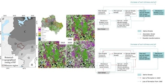
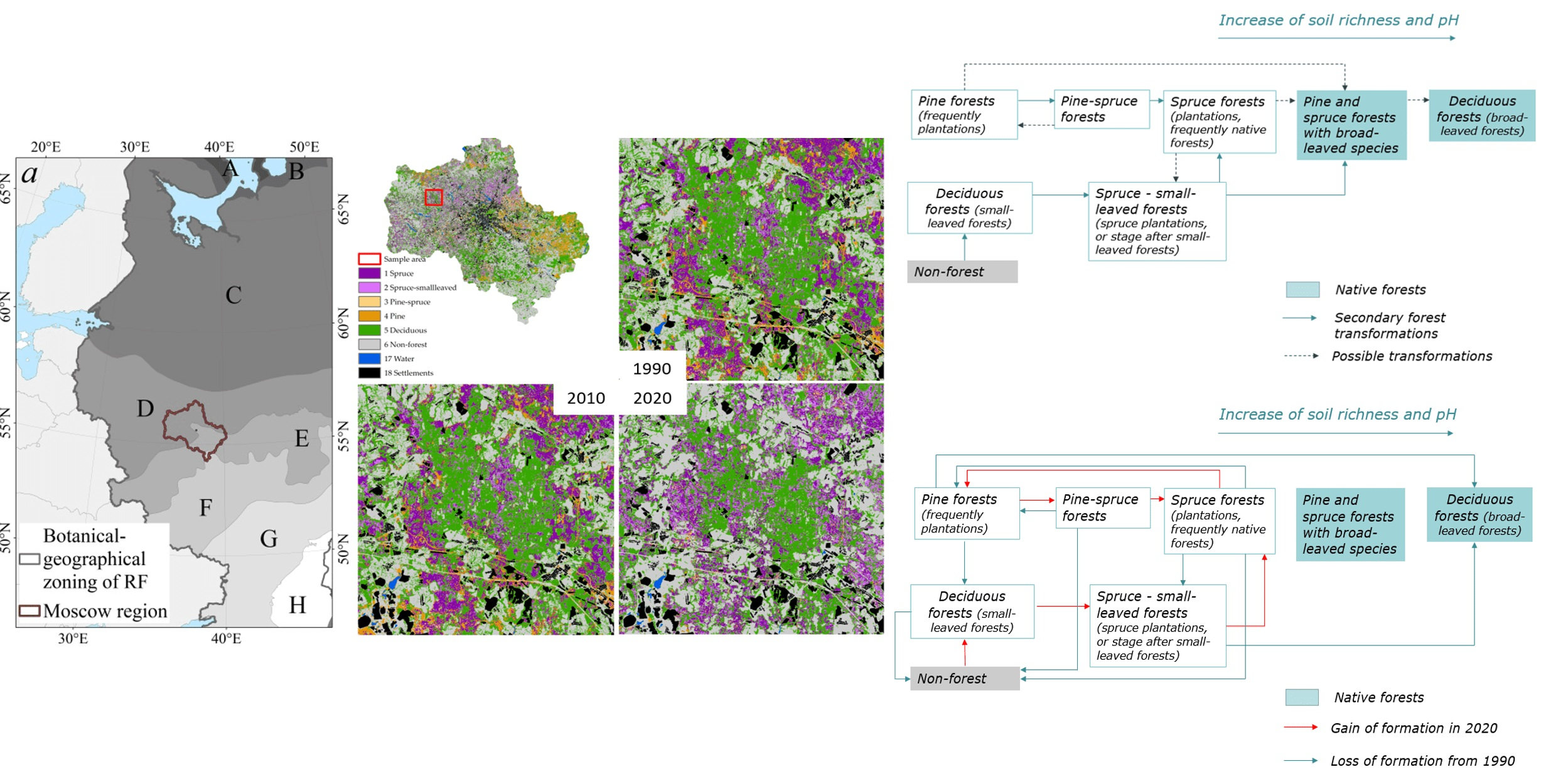
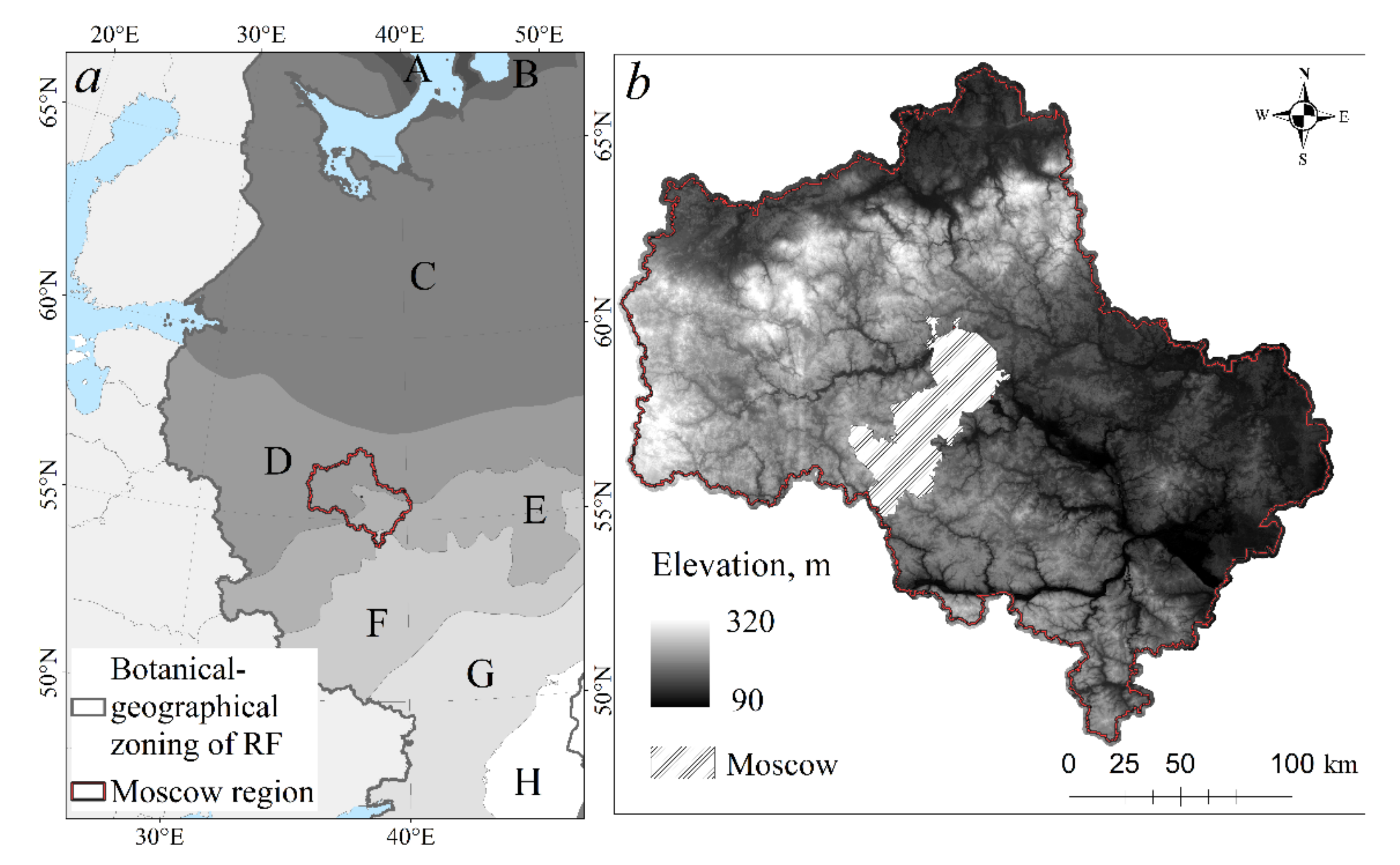
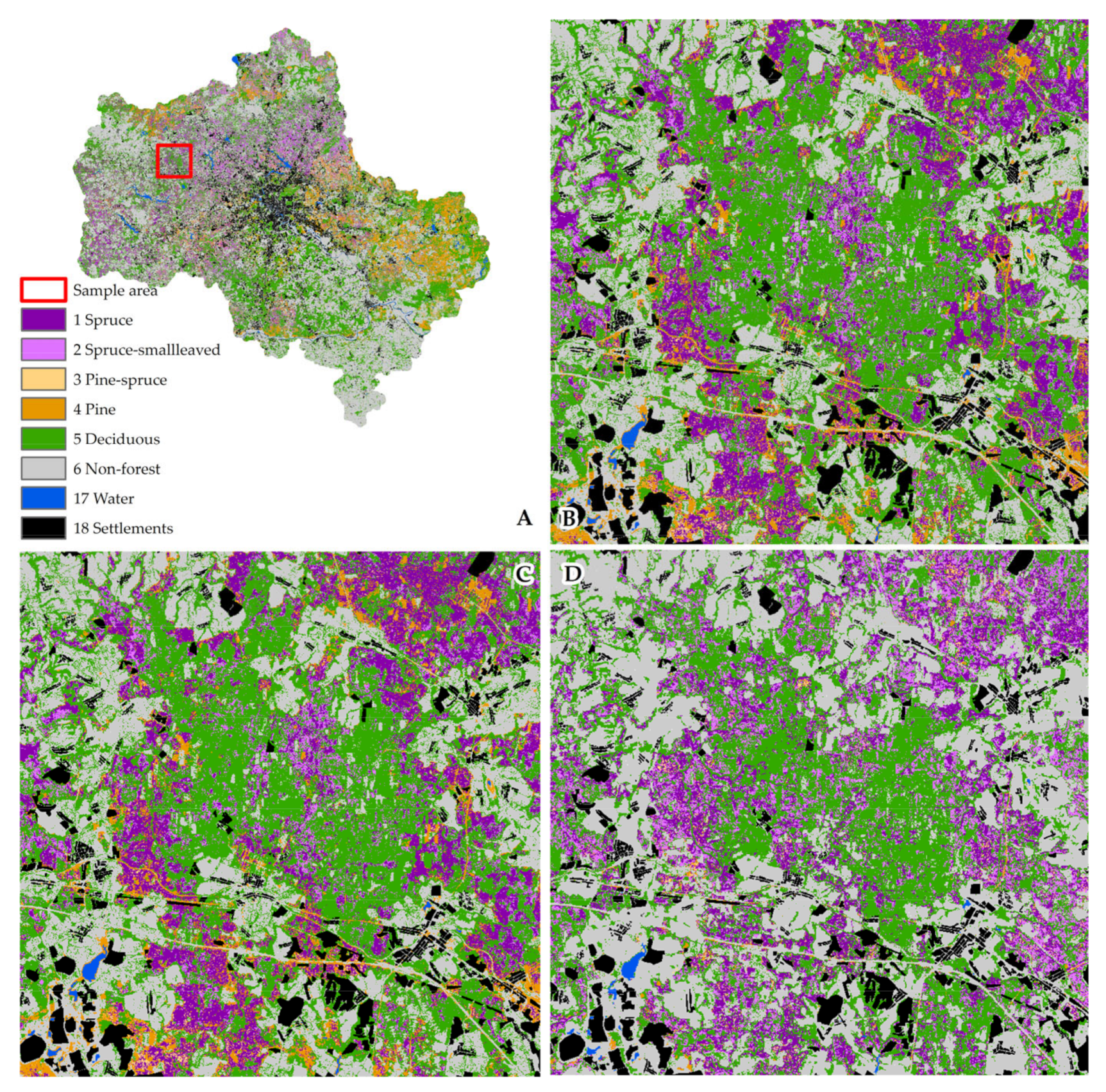
2.1. Study Area
2.2. The Main Trends of Forest Management and History of Coniferous Forests Formation
2.3. Methods
2.3.1. Field Data and Classification
- dwarf shrubs–small herb–green moss (#1—DshShG);
- small herb (#2—Sh);
- small herb–broad herb (#3—ShBh);
- broad herb (#4—Bh);
- meadow herb (#5—Mh);
- dwarf shrubs–herbal-sphagnum (#6—DshHSh).
2.3.2. Use of Remote Sensing Data
- Landsat 5 mosaicking for two periods: 2006–2012 (hereinafter 2010) and 1984–1990 (hereinafter 1990);
- Manual spatial rarefication of relevés which subject of forest loss and degradation;
- Testing of different models for best prediction of forest formations for the 2010;
- Creation of spectral signatures for the 2010 (training the classifier);
- Using the classifier on the 2010 mosaic;
- Using the classifier on the 1990 mosaic.
- 1984–1990, days of year: 120–260 (May 1–September 15), total 224 images (further referred as the “1990”), and
- 2006–2012, days of year: also 120–260, total of 175 images (further referred as the “2010”).
2.3.3. Specific Classification Algorithms
2.3.4. Quality Assessment and Additional Sources of Data
3. Results
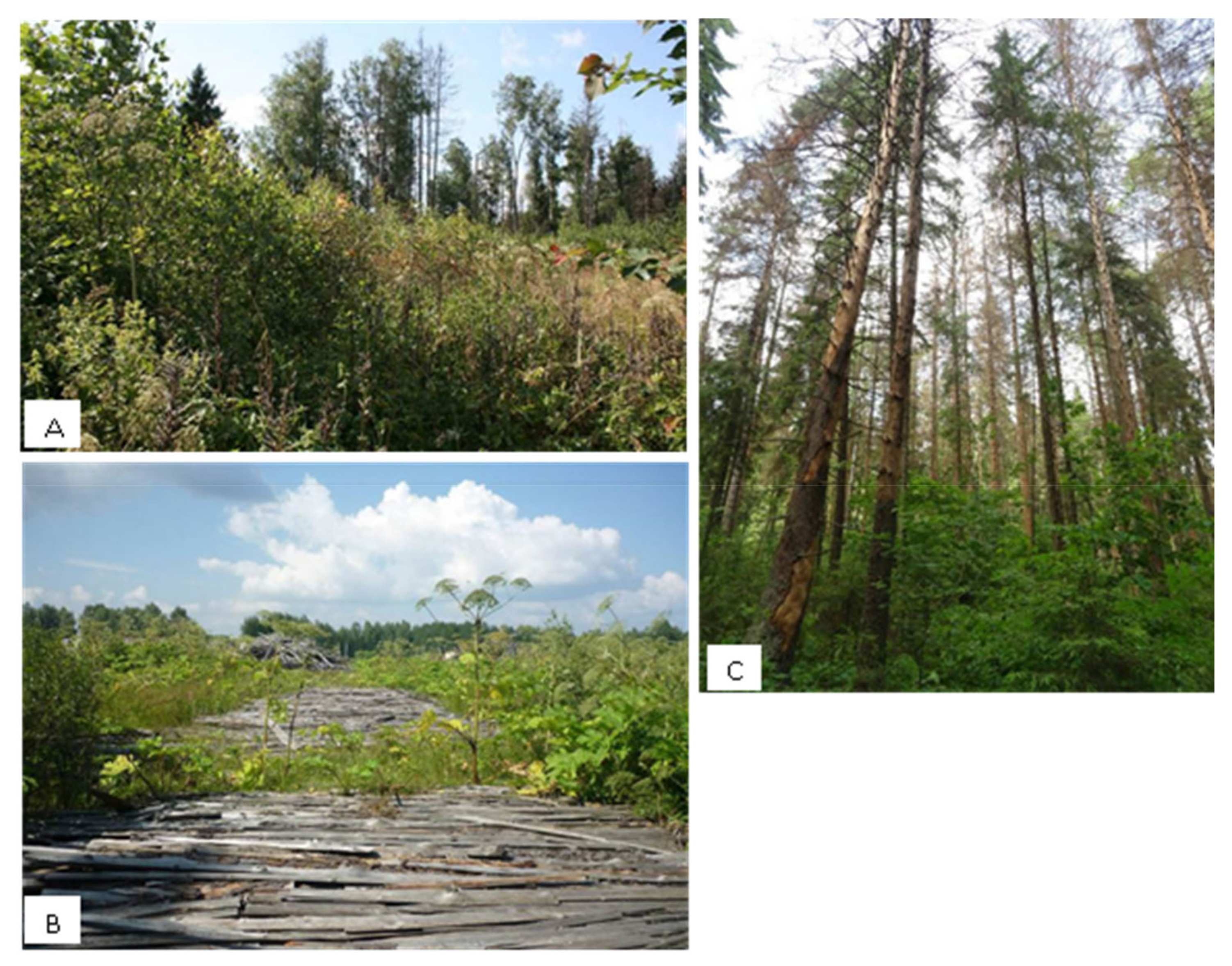
3.1. Characteristics of Present Spruce and Pine Forests

| Formation | Post Field Classification | Modeling | ||||
|---|---|---|---|---|---|---|
| Association Group | Number of Points | Number of Points | Train Sample | Test Sample | Proportion % | |
| Spruce | DshShG | 37 | 349 | 299 | 50 | |
| Sh | 40 | 14 | ||||
| ShBh | 148 | |||||
| Bh | 148 | |||||
| Spruce–small-leaved | DshShG | 32 | 219 | 179 | 40 | |
| Sh | 22 | 18 | ||||
| ShBh | 81 | |||||
| Bh | 102 | |||||
| Pine–spruce | DshShG | 32 | 122 | 107 | 10 | |
| Sh | 16 | 8 | ||||
| ShBh | 44 | |||||
| Bh | 42 | |||||
| Pine | DshShG | 46 | 216 | 176 | 40 | |
| Sh | 23 | |||||
| ShBh | 35 | 19 | ||||
| Bh | 64 | |||||
| Mh | 15 | |||||
| DshHSh | 45 | |||||
| Deciduous forests | 571 | 471 | 100 | 18 | ||
| Non-forest | 65 | 60 | 5 | 8 | ||
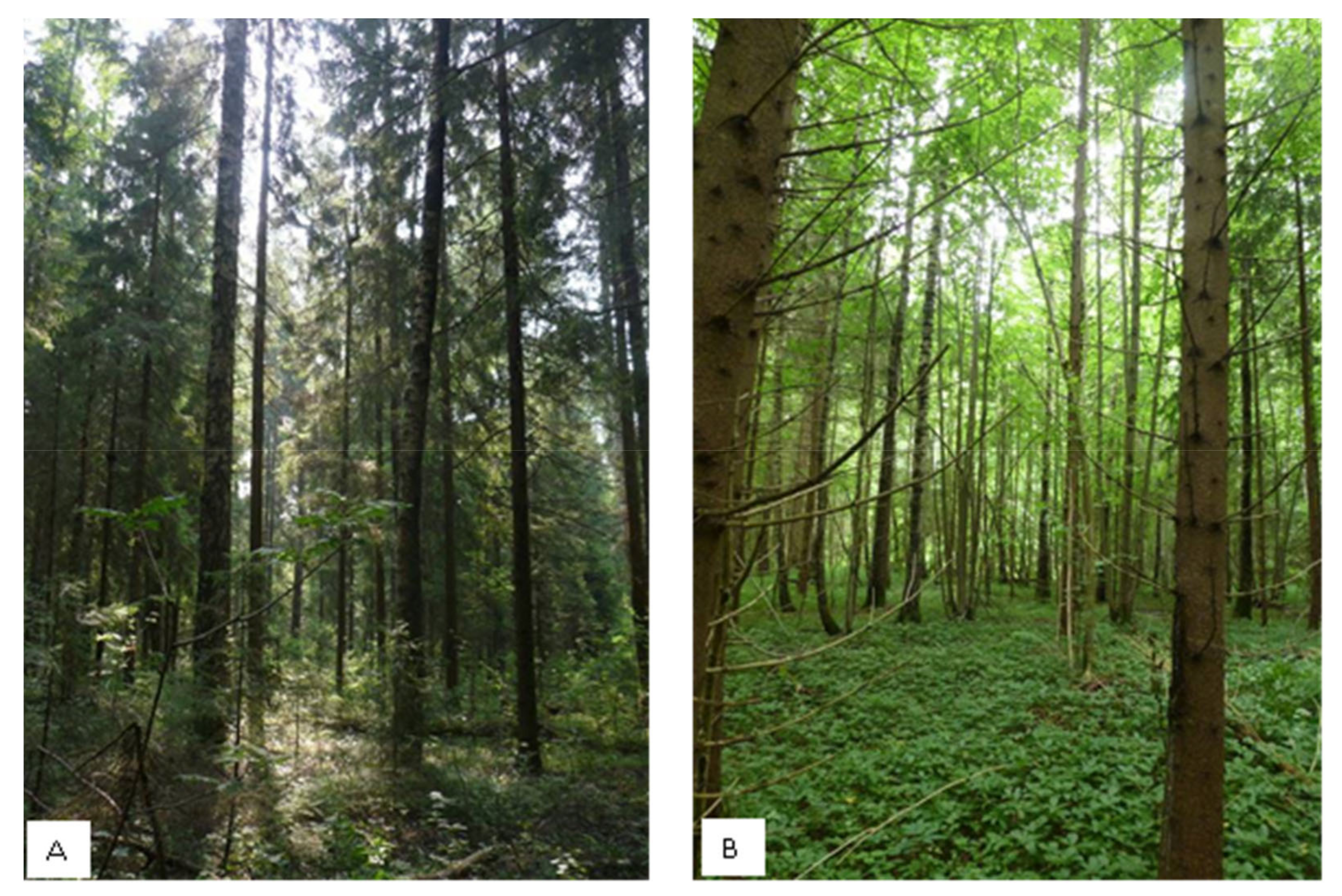
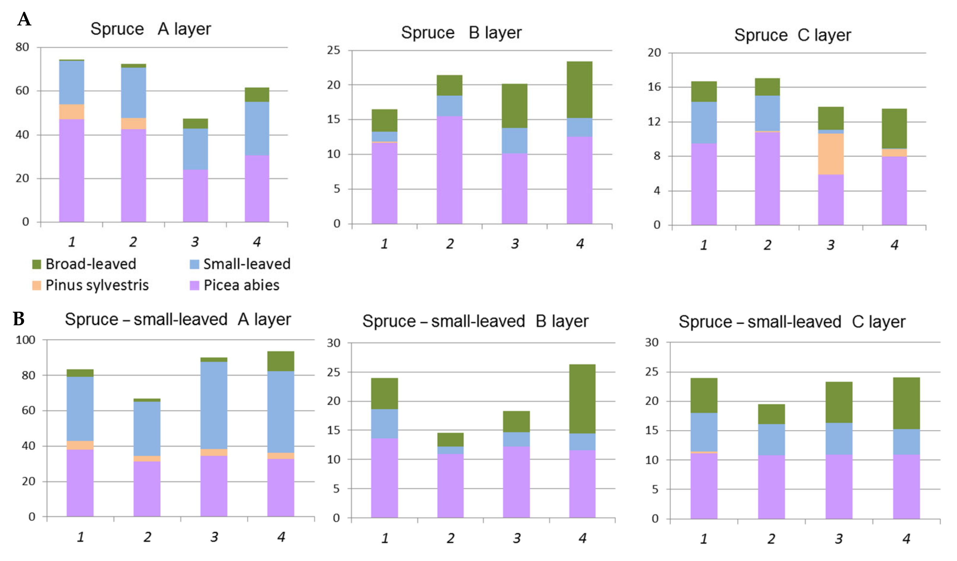
3.1.1. Spruce and Spruce–Small-Leaved Formations
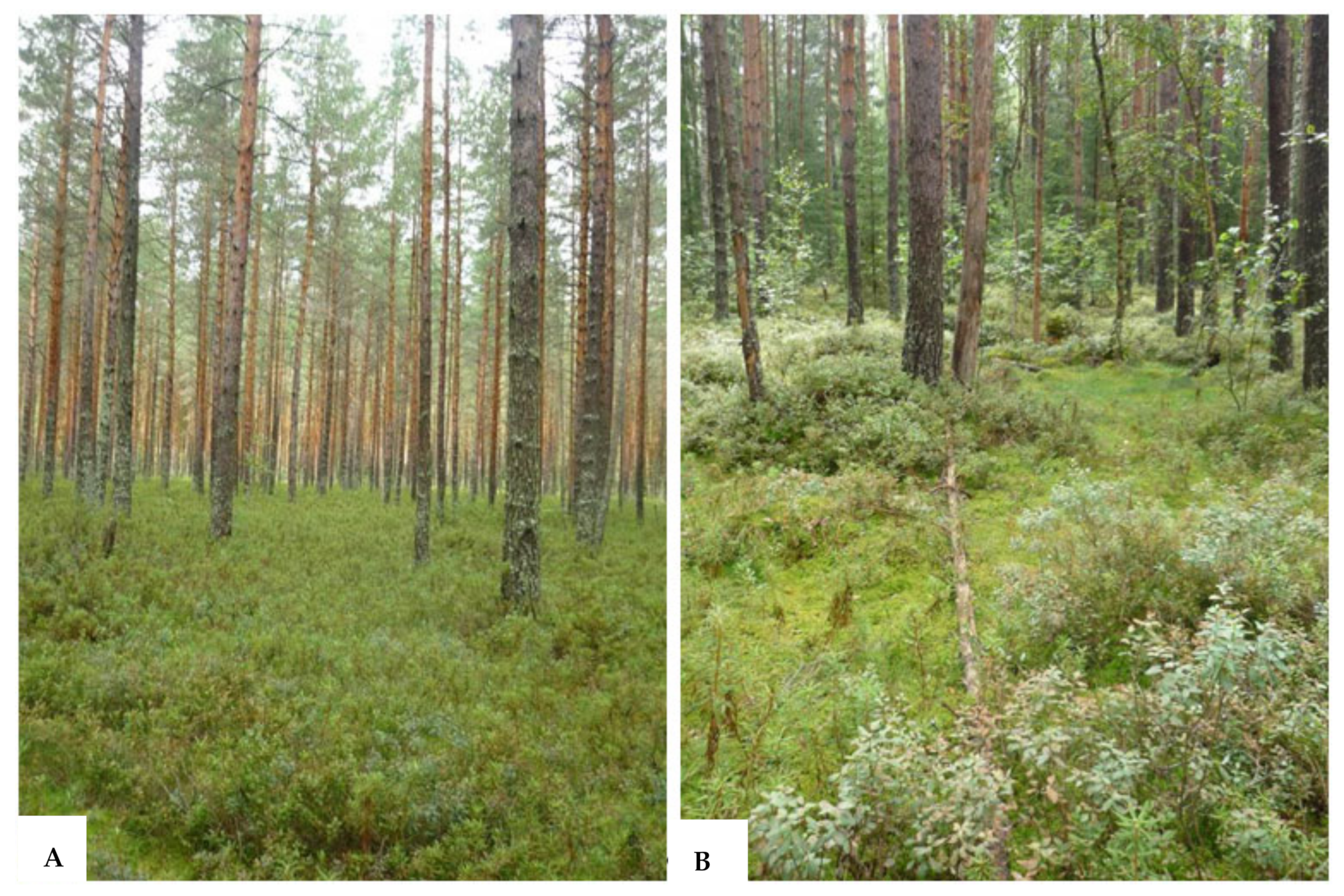
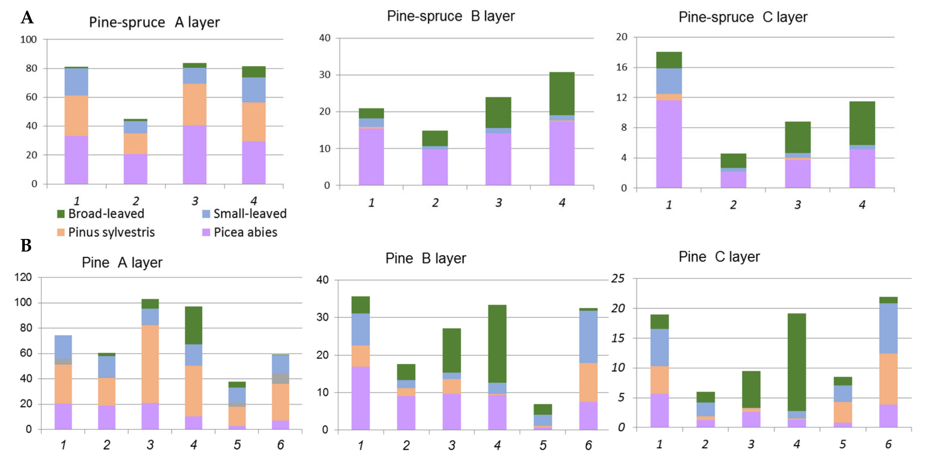
3.1.2. Pine and Pine-Spruce Formations
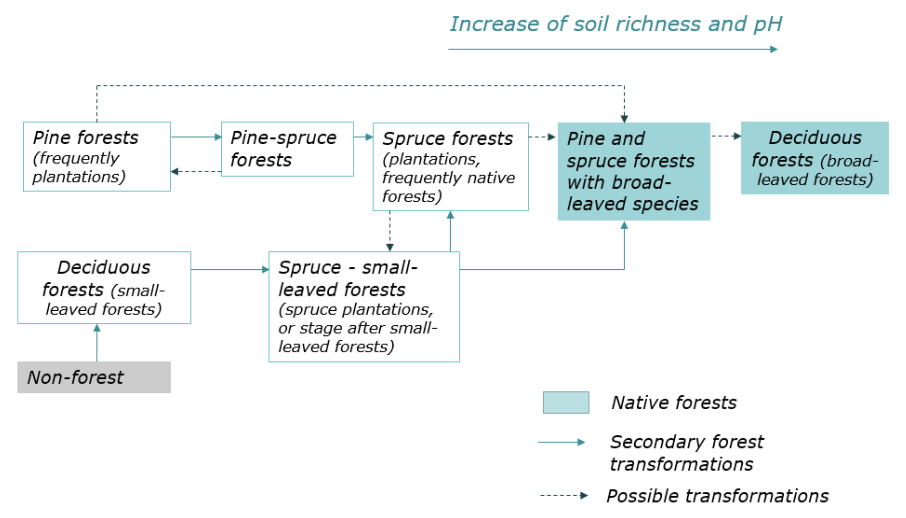
3.2. Dynamic Model of Coniferous Forests
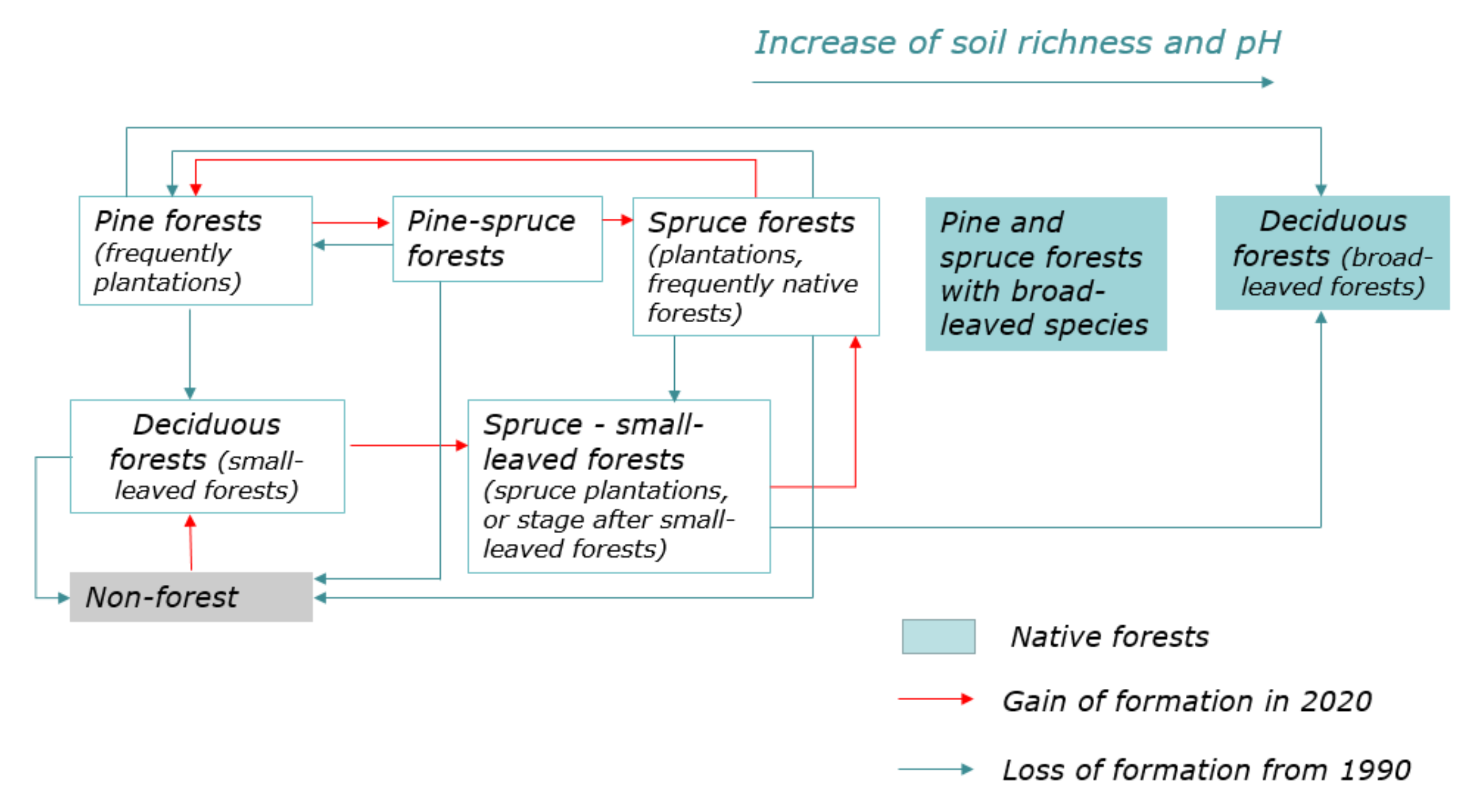
3.3. The Results of Retrospective Modeling 30 Years Ago
4. Discussion
5. Conclusions
Author Contributions
Funding
Data Availability Statement
Acknowledgments
Conflicts of Interest
Appendix A
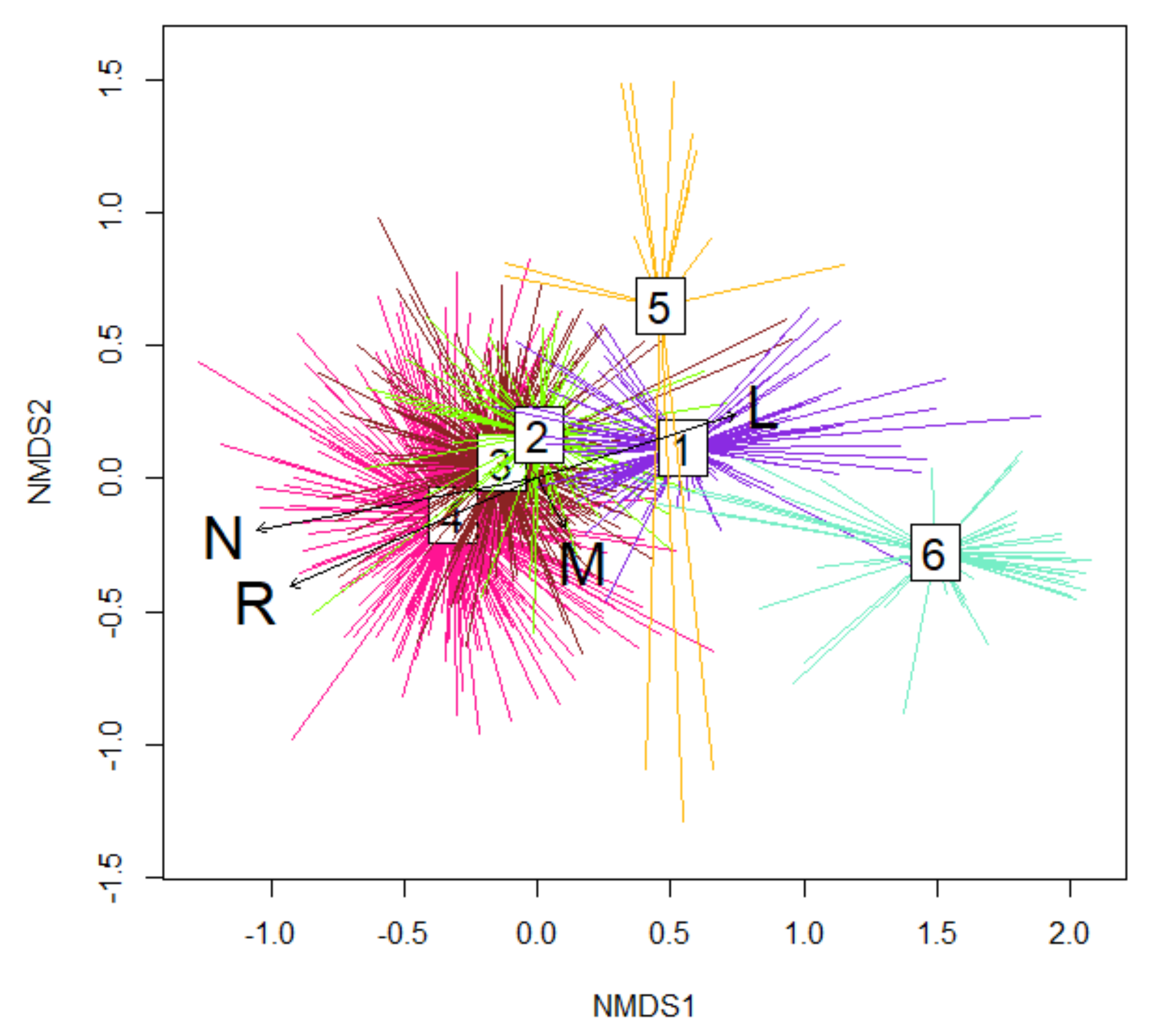
| Eecological Factors | NMDS1 | NMDS2 | R2 | pr (>r) |
|---|---|---|---|---|
| L | 0.95145 | 0.30779 | 0.3978 | 0.01 |
| R | −0.91634 | −0.40041 | 0.6658 | 0.01 |
| M | 0.48422 | −0.87495 | 0.0288 | 0.01 |
| N | −0.98414 | −0.17742 | 0.7424 | 0.01 |
| Community Group | |||||||
|---|---|---|---|---|---|---|---|
| #1—DshShG | #2—Sh | #3—ShBh | #4—Bh | ||||
| Species | IV | Species | IV | Species | IV | Species | IV |
| Pleurozium schreberi | 69 | Oxalis acetosella | 34 | Corylus avellana (B2) | 28 | Lamium galeobdolon | 45 |
| Vaccinium myrtillus | 60 | Mycelis muralis | 25 | Oxalis acetosella | 27 | Aegopodium podagraria | 43 |
| Hylocomium splendens | 52 | Ajuga reptans | 26 | Carex pilosa | 43 | ||
| Frangula alnus (B2) | 44 | Ranunculus cassubicus | 41 | ||||
| Vaccinium vitis-idaea | 39 | Corylus avellana (B2) | 37 | ||||
| Calamagrostis arundinacea | 37 | Pulmonaria obscura | 32 | ||||
| Orthilia secunda | 35 | Dryopteris filix-mas | 31 | ||||
| Luzula pilosa | 32 | Stellaria holostea | 31 | ||||
| Maianthemum bifolium | 30 | Asarum europaeum | 30 | ||||
| Trientalis europaea | 30 | ||||||
| Community Group | |||||||||||
|---|---|---|---|---|---|---|---|---|---|---|---|
| #1—DshShG | #2—Sh | #3—ShBh | #4—Bh | #5—Mh | #6—DshHSh | ||||||
| Species | IV | Species | IV | Species | IV | Species | IV | Species | IV | Species | IV |
| Pleurozium schreberi | 76 | Mycelis muralis | 43 | Corylus avellana B | 38 | Athyrium filix-femina | 48 | Trifolium medium | 67 | Eriophorum vaginatum | 71 |
| Vaccinium myrtillus | 59 | Oxalis acetosella | 42 | Dryopteris carthusiana | 36 | Ranunculus cassubicus | 36 | Calamagrostis arundinacea | 61 | Sphagnum magellanicum | 71 |
| Hylocomium splendens | 52 | Circaea alpina | 31 | Paris quadrifolia | 32 | Lamium galeobdolon | 32 | Agrimonia eupatoria | 58 | Ledum palustre | 57 |
| Dicranum polysetum | 50 | Sorbus aucuparia B | 30 | Viburnum opulus | 31 | Knautia arvensis | 58 | Vaccinium uliginosum | 57 | ||
| Picea abies C | 39 | Leucanthemum vulgare | 55 | Sphagnum angustifolium | 57 | ||||||
| Melampyrum pratense | 32 | Veronica officinalis | 51 | Vaccinium vitis-idaea | 55 | ||||||
| Clinopodium vulgare | 46 | Carex globularis | 54 | ||||||||
| Carex pallescens | 44 | Oxycoccus palustris | 43 | ||||||||
| Vicia cracca | 42 | Polytrichum strictum | 43 | ||||||||
| Campanula persicifolia | 41 | Aulacomnium palustre | 41 | ||||||||
| Fragaria vesca | 40 | Betula pubescens B | 38 | ||||||||
| Pinus sylvestris C | 37 | ||||||||||
| Lathyrus vernus | 35 | ||||||||||
| Melica nutans | 34 | ||||||||||
| Antennaria dioica | 33 | ||||||||||
| Astragalus glycyphyllos | 33 | ||||||||||
| Viola hirta | 33 | ||||||||||
| Chamaenerion angustifolium | 32 | ||||||||||
| 2020 | Loss of Forest Formation from Level 1990 | |||||||
|---|---|---|---|---|---|---|---|---|
| Formations | Spruce | Spruce–Small-Leaved | Pine–Spruce | Pine | Deciduous | Non-Forest | ||
| 1990 | Spruce | 13.1 | 16.3 | 6.1 | 28.0 | 14.7 | 21.7 | 86.9 |
| Spruce–small-leaved | 12.5 | 38.5 | 2.1 | 9.3 | 30.5 | 7.1 | 61.5 | |
| Pine-spruce | 10.5 | 7.5 | 10.9 | 29.0 | 12.6 | 29.4 | 89.1 | |
| Pine | 4.4 | 6.9 | 2.1 | 26.7 | 23.3 | 36.7 | 73.3 | |
| Deciduous | 2.9 | 14.4 | 0.3 | 3.5 | 58.4 | 20.5 | 41.6 | |
| Non-forest | 0.2 | 1.0 | 0.1 | 0.8 | 12.3 | 85.7 | 14.3 | |
| 2020 | |||||||
|---|---|---|---|---|---|---|---|
| Formations | Spruce | Spruce–Small-Leaved | Pine–Spruce | Pine | Deciduous | Non-Forest | |
| 1990 | Spruce | 42.8 | 20.7 | 56.1 | 40.3 | 6.0 | 5.9 |
| Spruce–small-leaved | 13.3 | 15.9 | 6.1 | 4.4 | 4.0 | 0.6 | |
| Pine-spruce | 3.3 | 0.9 | 9.7 | 4.0 | 0.5 | 0.8 | |
| Pine | 12.5 | 7.7 | 17.2 | 33.8 | 8.4 | 8.8 | |
| Deciduous | 26.2 | 51.1 | 7.8 | 14.2 | 66.4 | 15.5 | |
| Non-forest | 1.9 | 3.7 | 3.2 | 3.3 | 14.7 | 68.4 | |
| Gain of forest formation from level 2020 | 57.2% | 84.1% | 90.3% | 66.2% | 33.6% | 31.6% | |
| Month | 1 | 2 | 3 | 4 | 5 | 6 | 7 | 8 | 9 | 10 | 11 | 12 | Total |
|---|---|---|---|---|---|---|---|---|---|---|---|---|---|
| Total cloud cover | |||||||||||||
| Clear days | 1 | 2 | 4 | 3 | 4 | 2 | 2 | 3 | 2 | 2 | 1 | 1 | 27 |
| Cloudy days | 8 | 9 | 13 | 15 | 19 | 20 | 21 | 19 | 16 | 11 | 7 | 7 | 165 |
| Overcast days | 22 | 17 | 14 | 12 | 8 | 8 | 8 | 9 | 12 | 18 | 22 | 23 | 173 |
| Lower cloud cover | |||||||||||||
| Clear days | 5 | 7 | 10 | 9 | 8 | 5 | 6 | 8 | 8 | 5 | 3 | 3 | 77 |
| Cloudy days | 11 | 12 | 13 | 16 | 20 | 22 | 22 | 19 | 16 | 14 | 9 | 11 | 185 |
| Overcast days | 15 | 9 | 8 | 5 | 3 | 3 | 3 | 4 | 6 | 12 | 18 | 17 | 103 |
References
- Walter, H.; Box, E. Global classification of natural terrestrial ecosystems. Vegetation 1976, 32, 75–81. [Google Scholar] [CrossRef]
- Bailey, R.G. Ecoregions. In The Ecosystem Geography of the Oceans and Continents; Springer: New York, NY, USA, 2014; ISBN 978-1-4939-0524-9. [Google Scholar]
- Mücher, C.A.; Klijn, J.A.; Wascher, D.M.; Schaminée, J.H. A New European Landscape Classification (LANMAP): A Transparent, Flexible and User-Oriented Methodology to Distinguish Landscapes. Ecol. Indic. 2010, 10, 87–103. [Google Scholar] [CrossRef]
- Guerra, C.A.; Metzger, M.J.; Maes, J.; Pinto-Correia, T. Policy impacts on regulating ecosystem services: Looking at the implications of 60 years of landscape change on soil erosion prevention in a Mediterranean silvo-pastoral system. Landsc. Ecol. 2016, 31, 271–290. [Google Scholar] [CrossRef]
- Van Eetvelde, V.; Antrop, M. Landscape character beyond landscape typology: Methodological issues in trans-regional integration in Belgium. In Proceedings of the 18th International Annual ECLAS Conference: Landscape Assessment, from Theory to Practice: Applications in Planning and Design, Belgrade, Serbia, 10–14 October 2007; University of Belgrade: Belgrade, Serbia, 2007; pp. 229–239. [Google Scholar]
- Bailey, R.G. Ecosystem Geography: From Ecoregions to Sites; Springer: New York, NY, USA, 2009. [Google Scholar]
- Bai, F.; Sang, W.; Axmacher, J.C. Forest vegetation responses to climate and environmental change: A case study from Changbai Mountain, NE China. For. Ecol. Manag. 2011, 262, 2052–2060. [Google Scholar] [CrossRef]
- Zhang, K.; Kimball, J.S.; Nemani, R.R.; Running, S.W.; Hong, Y.; Gourley, J.J.; Yu, Z. Vegetation Greening and Climate Change Promote Multidecadal Rises of Global Land Evapotranspiration. Sci. Rep. 2015, 5, 15956. [Google Scholar] [CrossRef] [PubMed]
- Barbier, S.; Gosselin, F.; Balandier, P. Influence of tree species on understory vegetation diversity and mechanisms involved—A critical review for temperate and boreal forests. For. Ecol. Manag. 2008, 254, 1–15. [Google Scholar] [CrossRef]
- Cornwell, W.K.; Grubb, P.J. Regional and local patterns in plant species richness with respect to resource availability. Oikos 2003, 100, 417–428. [Google Scholar] [CrossRef] [Green Version]
- Spiecker, H. Silvicultural management in maintaining biodiversity and resistance of forests in Europe—Temperate zone. J. Environ. Manag. 2003, 67, 55–65. [Google Scholar] [CrossRef]
- Rysin, L.P. Lesa Podmoskovjia (Forests of Moscow Region); Tovarishhestvo Nauchnyh Izdanij KMK: Moscow, Russia, 2012. [Google Scholar]
- Rysin, L.P. Sukcessionnye processy v lesah central’noj chasti Russkoj ravniny (Successional processes in the forests of the central part of the Russian Plain). Usp. Sovrem. Biol. 2009, 578–587. [Google Scholar]
- Chernen’Kova, T.V.; Puzachenko, M.Y.; Belyaeva, N.G.; Kotlov, I.P.; Morozova, O.V. Pine Forests in Moscow Region: History and Perspectives of Preservation. Contemp. Probl. Ecol. 2019, 12, 711–723. [Google Scholar] [CrossRef]
- Cvetkov, M.A. Izmenenie Lesistosti Evropejskoj Rossii S Konca XVII Stoletija Po 1914 God (Forest Cover Change of European Russia from the End of the XVII Century to 1914); USSR Academy of Sciences Publishing House: Moscow, Russia, 1957. [Google Scholar]
- Osipov, V.V.; Gavrilova, N.K. Agrarnoe Osvoenie i Dinamika Lesistosti Nechernozemnoj Zony RSFSR (Agricultural Development and Dynamics of Forest Cover of Nonchernozem Belt of RSFSR); Nauka: Russia, Moscow, 1983. [Google Scholar]
- Hansen, M.C.; Potapov, P.V.; Moore, R.; Hancher, M.; Turubanova, S.A.; Tyukavina, A.; Thau, D.; Stehman, S.V.; Goetz, S.J.; Loveland, T.R. High-Resolution Global Maps of 21st-Century Forest Cover Change. Science 2013, 342, 850–853. [Google Scholar] [CrossRef] [Green Version]
- Turubanova, S.A.; Krylov, A.M.; Potapov, P.V.; Tyukavina, A.Y. Forest Dynamics in Eastern Europe (1985–2012) Using Landsat Data Archive. Russ. J. Ecosyst. Ecol. 2017, 2. [Google Scholar] [CrossRef] [Green Version]
- Lyubimova, E.L. Description of vegetation of natural areas of Moscow oblast. In Ocherki Prirody Podmoskov’ya (Reviews of The Nature in Moscow Region); Akademii Nauk SSSR: Moscow, Russia, 1957; pp. 42–82. [Google Scholar]
- Kurnaev, S.F. Osnovnye Tipy Lesa Srednej Chasti Russkoj Ravniny (Main Forest Types of Russian Plain Middle Part); Nauka: Moscow, Russia, 1968. [Google Scholar]
- Rysin, L.P. Lesa Vostochnogo Podmoskov’ya (Forests of Eastern Part of Moscow Region); Nauka: Moscow, Russia, 1979. [Google Scholar]
- Smagin, V.N. Biogeotsenologicheskie Osnovy Sozdaniya Prirodnykh Zakaznikov (Na Primere Zakaznika “Verkhnaya Moskva Reka”)(Biogeocenologic Principles of Organization of Natural Wildlife Sanctuaries by Example of Verkhnyaya Moskva-Reka Wildlife Sanctuary); Nauka: Moscow, Russia, 1980. [Google Scholar]
- Il’inskaya, S.A.; Matveeva, M.A.; Rechan, S.P.; Kazantceva, T.N.; Orlova, M.A. Tipy lesa (Forest types). In Lesa Zapadnogo Podmoskov’ja (Forests of the Western Moscow Region); Nauka: Moscow, Russia, 1982; pp. 20–149. [Google Scholar]
- Rysin, L.P. Lesa Zapadnogo Podmoskov’ya (Forests of Western Part of Moscow Region); Nauka: Moscow, Russia, 1982. [Google Scholar]
- Rysin, L.P. Lesa Yuzhnogo Podmoskov’ya (Forests of Southern Part of Moscow Region); Nauka: Moscow, Russia, 1985. [Google Scholar]
- Rysin, L.P. Natural conditions in Moscow region. In Dinamika khvoinykh lesov Podmoskov’ya (Dynamics of Coniferous Forests in Moscow Region); Nauka: Moscow, Russia, 2000; pp. 5–21. [Google Scholar]
- Chernenkova, T.V.; Suslova, E.G.; Morozova, O.V.; Belyaeva, N.G.; Kotlov, I.P. Bioraznoobrazie Lesov Moskovskogo Regiona (Forest Biodiversity of Moscow Region). Ecosyst. Ecol. Dyn. 2020, 4, 60–144. [Google Scholar] [CrossRef]
- Ogureeva, G.N.; Miklyaeva, I.M.; Suslova, E.G.; Shvergunova, L.V. Rastitel’nost’ Moskovskoj Oblasti (Vegetation of Moscow Region); EKOR: Moscow, Russia, 1996. [Google Scholar]
- Giri, C.P. Remote Sensing of Land Use and Land Cover: Principles and Applications; CRC Press: Boca Raton, FL, USA, 2012. [Google Scholar]
- Keenan, R.J.; Reams, G.A.; Achard, F.; de Freitas, J.V.; Grainger, A.; Lindquist, E. Dynamics of global forest area: Results from the FAO Global Forest Resources Assessment 2015. For. Ecol. Manag. 2015, 352, 9–20. [Google Scholar] [CrossRef]
- Song, X.-P.; Hansen, M.C.; Stehman, S.V.; Potapov, P.V.; Tyukavina, A.; Vermote, E.F.; Townshend, J.R. Global land change from 1982 to 2016. Nat. Cell Biol. 2018, 560, 639–643. [Google Scholar] [CrossRef]
- Yin, H.; Pflugmacher, D.; Li, A.; Li, Z.; Hostert, P. Land use and land cover change in Inner Mongolia - understanding the effects of China’s re-vegetation programs. Remote Sens. Environ. 2018, 204, 918–930. [Google Scholar] [CrossRef]
- Zhou, D.; Zhao, S.; Zhu, C. The Grain for Green Project induced land cover change in the Loess Plateau: A case study with Ansai County, Shanxi Province, China. Ecol. Indic. 2012, 23, 88–94. [Google Scholar] [CrossRef]
- Gutman, G.; Radeloff, V. Land-Cover and Land-Use Changes in Eastern Europe after the Collapse of the Soviet Union in 1991; Springer: Berlin/Heidelberg, Germany, 2016; ISBN 3-319-42638-9. [Google Scholar]
- Abad-Segura, E.; González-Zamar, M.-D.; Vázquez-Cano, E.; López-Meneses, E. Remote Sensing Applied in Forest Management to Optimize Ecosystem Services: Advances in Research. Forests 2020, 11, 969. [Google Scholar] [CrossRef]
- Brooks, B.-G.J.; Lee, D.C.; Pomara, L.Y.; Hargrove, W.W. Monitoring Broadscale Vegetational Diversity and Change across North American Landscapes Using Land Surface Phenology. Forests 2020, 11, 606. [Google Scholar] [CrossRef]
- Kennedy, R.E.; Yang, Z.G.; Cohen, W.B. Detecting trends in forest disturbance and recovery using yearly Landsat time series: 1. LandTrendr—Temporal segmentation algorithms. Remote Sens. Environ. 2010, 114, 2897–2910. [Google Scholar] [CrossRef]
- Cochran, F.; Daniel, J.; Jackson, L.; Neale, A. Earth observation-based ecosystem services indicators for national and subnational reporting of the sustainable development goals. Remote Sens. Environ. 2020, 244, 111796. [Google Scholar] [CrossRef]
- Barbierato, E.; Bernetti, I.; Capecchi, I.; Saragosa, C. Integrating Remote Sensing and Street View Images to Quantify Urban Forest Ecosystem Services. Remote Sens. 2020, 12, 329. [Google Scholar] [CrossRef] [Green Version]
- Wang, C.; Zhao, H. Analysis of remote sensing time-series data to foster ecosystem sustainability: Use of temporal information entropy. Int. J. Remote Sens. 2018, 40, 2880–2894. [Google Scholar] [CrossRef]
- Mohren, G. Large-scale scenario analysis in forest ecology and forest management. For. Policy Econ. 2003, 5, 103–110. [Google Scholar] [CrossRef]
- Ochtyra, A.; Marcinkowska-Ochtyra, A.; Raczko, E. Threshold- and trend-based vegetation change monitoring algorithm based on the inter-annual multi-temporal normalized difference moisture index series: A case study of the Tatra Mountains. Remote Sens. Environ. 2020, 249, 112026. [Google Scholar] [CrossRef]
- Greig, C.; Robertson, C.; Lacerda, A.E. Spectral-temporal modelling of bamboo-dominated forest succession in the Atlantic Forest of Southern Brazil. Ecol. Model. 2018, 384, 316–332. [Google Scholar] [CrossRef]
- Liu, L.; Zhang, X.; Hu, Y.; Wang, Y. Automatic land cover mapping for Landsat data based on the time-series spectral image database. IEEE Int. Geosci. Remote Sens. Symp. 2017, 4282–4285. [Google Scholar] [CrossRef]
- Kurnaev, S.F. Lesorastitel’noe Rajonirovanie SSSR (Forest Zoning of the USSR); Nauka: Moscow, Russia, 1973. [Google Scholar]
- Rivas-Martínez, S.; Penas, A.; Díaz, T.E. Mapas Bioclimáticos y Biogeográficos. Available online: https://www.globalbioclimatics.org/form/bi_med.htm (accessed on 7 December 2020).
- Litvinenko, L.N.; Kalinina, A.A. Raspredelenie Osadkov Na Territorii Moskovskoj Oblasti Pri Nalichii i Otsutstvii Krupnogo Antropogennogo Obrazovanija (Distribution of Precipitation on the Territory of the Moscow Region in the Presence and Absence of a Large Anthropogenic Formation). Ecol. Urban. Areas 2018. [Google Scholar] [CrossRef]
- Spiridonov, A.I. Kraevye Obrazovanija Moskovskogo Oledenenija v Central’nyh Oblastjah Russkoj Ravniny (Edge Formations of the Moscow Glaciation in the Central Regions of the Russian Plain); Nauka: Moscow, Russia, 1972. [Google Scholar]
- Petrov, V.V. Novaja Shema Geobotanicheskogo Rajonirovanija Moskovskoj Oblasti (New Scheme of Geobotanical Zoning of the Moscow Region). Vestnik Moskovskogo Gosudarstvennogo Universiteta Biol. Pochvovedenie 1968, 44–49. [Google Scholar]
- Ogureeva, G.N. Zony i Tipy Pojasnosti Rastitel’nosti Rossii (Zones and Types of Vegetation Zonation in Russia). Available online: http://byrranga.ru/docs/277.pdf (accessed on 9 December 2020).
- Lesnoj Plan Moskovskoj Oblasti Kniga 1 (Forest Plan of the Moscow Region Book 1); Federal Forestry Agency, Government of the Russian Federation: Moscow, Russia, 2010.
- Rysin, L.P.; Abaturov, A.V.; Savel’eva, L.I. Dinamika Hvojnyh Lesov Podmoskov’ja (Dynamic of Coniferous Forests of Moscow Region); Nauka: Moscow, Russia, 2000; ISBN 5-02-004435-0. [Google Scholar]
- Abaturov, A.V.; Melanholin, P.N. Estestvennaja Dinamika Lesa Na Postojannyh Probnyh Ploshhadjah v Podmoskov’e (Natural Forest Dynamics on Permanent Test Plots in the Moscow Region); Grif i K: Tula, Russia, 2004; ISBN 5-8125-0472-5. [Google Scholar]
- Rysin, L.P.; Savel’eva, L.I. Kadastry Tipov Lesa I Tipov Lesnyh Biogeocenozov (Cadastres of Forest Types and Types of Forest Biodeosenoses); Tovarishhestvo Nauchnyh Izdanij KMK: Moscow, Russia, 2007; ISBN 978-5-87317-397-6. [Google Scholar]
- Bobrovsky, M.V. Lesnye Pochvy Evropeiskoi Rossii: Bioticheskie i Antropogennye Faktory Formirovaniya (Forest Soil in European Russia: Biotic and Anthropogenic Factors in Pedogenesis); KMK: Moscow, Russia, 2010; ISBN 978-5-87317-733-2. [Google Scholar]
- Nizovtsev, V.A.; Marchenko, N.A.; Onishchenko, M.V.; Галкин, Ю.С. Istoricheskaya Dinamika Zemlepol’zovaniya v Landshaftakh Tsentral’noi Rossii (History Dynamics of Land-Use of Central Russian Landscapes). In Proceedings of the Ecology of River’s Basins, Vladimir, Russia, 28–30 September 2007; pp. 146–151. [Google Scholar]
- Abaturov, A.V. Iz istorii lesov Podmoskov’ja (From the history of the forests of the Moscow region). In Dinamika Hvojnyh Lesov Podmoskov’ja (Dynamic of Coniferous Forests of Moscow Region); Nauka: Moscow, Russia, 2000; pp. 22–32. ISBN 5-02-004435-0. [Google Scholar]
- Milov, L.V. Velikorusskii Pakhar’ i Osobennosti Rossiiskogo Istoricheskogo Protsessa (Great Russian Plowman and Features of Russian History); ROSSPEN: Moscow, Russia, 2006; ISBN 5-86004-131-4. [Google Scholar]
- Pushkarev, S.G. Rossiya v XIX Veke (1801–1914) (Russia in the XIX Century (1801–1904); izd-vo im. A.P.Chekhova: New York, NY, USA, 1956. [Google Scholar]
- Karimov, A.E. Dokuda Topor i Sokha Khodili. Ocherki Istorii Zemel’nogo i Lesnogo Kadastra v Rossii XVI- Nachala XX Veka (Countryside, Shaped by Ax and Plough. History Studies of Land and Forest Registry of Russia in the XVI–Early XX Century); Nauka: Moscow, Russia, 2007; ISBN 978-5-02-034114-2. [Google Scholar]
- Ceplyaev, V.P. Lesa SSSR (Hozjajstvennaja Harakteristika) (Forests of the USSR (Economic Characteristics)); Selhozgiz: Moscow, Russia, 1961. [Google Scholar]
- Bjudzhet Dlja Grazhdan (Budget for Citizens). Available online: https://budget.mosreg.ru/download/Byudjet_dlya_grajdan(2)/BdG-proekt-20-22-.pdf (accessed on 13 December 2020).
- Merzlenko, M.D. Starejshie Iskusstvennye Lesa Podmoskov’ja (The Oldest Plantations in the Moscow Region). Priroda 1978, 10, 50–57. [Google Scholar]
- Markova, I.A. Sovremennye Problemy Lesovyrashhisvanija (Lesokul’turnoe Proizvodstvo): Uchebnoe Posobie (Modern Problems of Forest Planting (Forest Production): Textbook); SPbLTA: Sankt-Peterburg, Russia, 2008; ISBN 978-5-9239-0153-5. [Google Scholar]
- Shutov, I.V. Plantacionnoe Lesovodstvo (Plantation Forestry); Polytechnic University Publishing House: Sankt-Peterburg, Russia, 2007; ISBN 5-7422-1714-5. [Google Scholar]
- Obzor Lesopatologicheskogo i Sanitarnogo Sostojanija Lesov v Moskovskoj Oblasti v 2009 Godu i Prognoz Lesopatologicheskoj Situacii Na 2010 God (Review of Forest Pathological and Sanitary State of Forests in the Moscow Region in 2009 and Forecast of Forest Pathological Situation for 2010); Federal Forestry Agency: Puschino, Russia, 2010.
- Hlásny, T.; Krokene, P.; Liebhold, A.; Montagné-Huck, C.; Müller, J.; Qin, H.; Raffa, K.; Schelhaas, M.-J.; Seidl, R.; Svoboda, M.; et al. Living with Bark Beetles: Impacts, Outlook and Management Options; From Science to Policy; European Forest Institute: Joensuu, Finland, 2019; Available online: https://efi.int/sites/default/files/files/publication-bank/2019/efi_fstp_8_2019_0.pdf (accessed on 7 May 2021).
- Venäläinen, A.; Lehtonen, I.; Laapas, M.; Ruosteenoja, K.; Tikkanen, O.; Viiri, H.; Ikonen, V.; Peltola, H. Climate change induces multiple risks to boreal forests and forestry in Finland: A literature review. Glob. Chang. Biol. 2020, 26, 4178–4196. [Google Scholar] [CrossRef]
- Maslov, A.D. Koroed-Tipograf i Usyhanie Elovyh Lesov (Bark Beetle Typographer and Drying up of Spruce Forests); Vserossijskij nauchno-issledovatel’skij institut lesovodstva i mehanizacii lesnogo hozjajstva: Pushkino, Russia, 2010; ISBN 978-5-94219-170-2. [Google Scholar]
- Braun-Blanquet, J. Pflanzensoziologie, 3rd ed.; Springer: Vienna, Austria; New York, NY, USA, 1964. [Google Scholar]
- Chernen’Kova, T.V.; Morozova, O.V. Classification and Mapping of Coenotic Diversity of Forests. Contemp. Probl. Ecol. 2017, 10, 738–747. [Google Scholar] [CrossRef]
- Chernenkova, T.; Kotlov, I.; Belyaeva, N.; Suslova, E.; Morozova, O.; Pesterova, O.; Arkhipova, M. Role of Silviculture in the Formation of Norway Spruce Forests along the Southern Edge of Their Range in the Central Russian Plain. Forests 2020, 11, 778. [Google Scholar] [CrossRef]
- Malyshev, L.I. Floristicheskoe Rajonirovanie Na Osnove Kolichestvennyh Priznakov. Florist. Zoning Based Quant. Charact. 1973, 58, 1581–1588. [Google Scholar]
- European Environment Agency. R Core Team. 2020. Available online: https://www.eea.europa.eu/data-and-maps/indicators/oxygen-consuming-substances-in-rivers/r-development-core-team-2006 (accessed on 13 December 2020).
- Oksanen, J.; Blanchet, F.G.; Kindt, R.; Legendre, P.; Minchin, P.R.; O’hara, R.B.; Simpson, G.L.; Solymos, P.; Stevens, M.H.H.; Wagner, H. Package ‘Vegan’. Community Ecol. Package 2013, 2, 1–295. [Google Scholar]
- Düll, R. Zeigerwerte von Laub-Und Lebermoosen. Scr. Geobot. 1991, 18, 175–214. [Google Scholar]
- Ellenberg, H.; Weber, H.E.; Düll, R.; Wirth, V.; Werner, W.; Paulissen, D. Zeigerwerte von Pflanzen in Mitteleuropa. Scr. Geobot. 1991, 18, 1–248. [Google Scholar]
- Tichý, L. JUICE, Software for Vegetation Classification. J. Veg. Sci. 2002, 13, 451–453. [Google Scholar] [CrossRef]
- Strahler, A.H.; Muller, J.; Lucht, W.; Schaaf, C.; Tsang, T.; Gao, F.; Li, X.; Lewis, P.; Barnsley, M.J. MODIS BRDF/Albedo Product: Algorithm Theoretical Basis Document Version 5.0. MODIS Doc. 1999, 23, 42–47. [Google Scholar]
- Housman, I.W.; Chastain, R.A.; Finco, M.V. An Evaluation of Forest Health Insect and Disease Survey Data and Satellite-Based Remote Sensing Forest Change Detection Methods: Case Studies in the United States. Remote Sens. 2018, 10, 1184. [Google Scholar] [CrossRef] [Green Version]
- Gorelick, N.; Hancher, M.; Dixon, M.; Ilyushchenko, S.; Thau, D.; Moore, R. Google Earth Engine: Planetary-scale geospatial analysis for everyone. Remote Sens. Environ. 2017, 202, 18–27. [Google Scholar] [CrossRef]
- Script for Landsat 5 Mosaicking. Available online: https://code.earthengine.google.com/?scriptPath=users%2Fikotlov%2FALL%3ALandsat5mosaic2_1990 (accessed on 7 May 2021).
- Masek, J.; Vermote, E.; Saleous, N.; Wolfe, R.; Hall, F.; Huemmrich, K.; Gao, F.; Kutler, J.; Lim, T.-K. A Landsat Surface Reflectance Dataset for North America, 1990–2000. IEEE Geosci. Remote Sens. Lett. 2006, 3, 68–72. [Google Scholar] [CrossRef]
- Kotlov, I.; Chernenkova, T. Modeling of Forest Communities’ Spatial Structure at the Regional Level through Remote Sensing and Field Sampling: Constraints and Solutions. Forests 2020, 11, 1088. [Google Scholar] [CrossRef]
- Inglada, J.; Christophe, E. The Orfeo Toolbox remote sensing image processing software. In Proceedings of the 2009 IEEE International Geoscience and Remote Sensing Symposium 2009, Cape Town, South Africa, 12–17 July 2009; Volume 4, pp. 733–736. [Google Scholar] [CrossRef]
- Grabska, E.; Frantz, D.; Ostapowicz, K. Evaluation of machine learning algorithms for forest stand species mapping using Sentinel-2 imagery and environmental data in the Polish Carpathians. Remote. Sens. Environ. 2020, 251, 112103. [Google Scholar] [CrossRef]
- Liu, Q.; Huang, C.; Li, H. Mapping plant communities within quasi-circular vegetation patches using tasseled cap brightness, greenness, and topsoil grain size index derived from GF-1 imagery. Earth Sci. Inform. 2021, 1–10. [Google Scholar] [CrossRef]
- Breiman, L. Random Forests. Mach. Learn. 2001, 45, 5–32. [Google Scholar] [CrossRef] [Green Version]
- Furuya, D.; Aguiar, J.; Estrabis, N.; Pinheiro, M.; Furuya, M.; Pereira, D.; Gonçalves, W.; Liesenberg, V.; Li, J.; Junior, J.M.; et al. A Machine Learning Approach for Mapping Forest Vegetation in Riparian Zones in an Atlantic Biome Environment Using Sentinel-2 Imagery. Remote Sens. 2020, 12, 4086. [Google Scholar] [CrossRef]
- Altman, N.S. An Introduction to Kernel and Nearest-Neighbor Nonparametric Regression. Am. Stat. 1992, 46, 175–185. [Google Scholar] [CrossRef] [Green Version]
- Stehman, S. Estimating the Kappa Coefficient and Its Variance under Stratified Random Sampling. Photogramm. Eng. Remote Sens. 1996, 62, 401–407. [Google Scholar]
- Radosavljevic, A.; Anderson, R.P. Making better Maxent models of species distributions: Complexity, overfitting and evaluation. J. Biogeogr. 2014, 41, 629–643. [Google Scholar] [CrossRef]
- Shcheglovitova, M.; Anderson, R.P. Estimating optimal complexity for ecological niche models: A jackknife approach for species with small sample sizes. Ecol. Model. 2013, 269, 9–17. [Google Scholar] [CrossRef]
- Landis, J.R.; Koch, G.G. The Measurement of Observer Agreement for Categorical Data. Biometrics 1977, 33, 159–174. [Google Scholar] [CrossRef] [PubMed] [Green Version]
- Savel’eva, L.I. Tipy hvojnyh lesov Podmoskov’ja (Types of coniferous forests in the Moscow region). In Dinamika hvojnyh lesov Podmoskov’ja (Dynamics of coniferous forests in the Moscow region); Nauka: Moscow, Russia, 2000; p. 221. ISBN 5-02-004435-0. [Google Scholar]
- Rysin, L.P.; Savel’eva, L.I. Elovye Lesa Rossii (Spruce Forests of Russia); Nauka: Moscow, Russia, 2002; ISBN 5-02-006501-3. [Google Scholar]
- Rysin, L.P.; Savel’eva, L.I. Sosnovye Lesa Rossii (Pine Forests of Russia); Tovarishhestvo nauchnyh izdanij KMK: Moscow, Russia, 2008; ISBN 978-5-87317-512-3. [Google Scholar]
- Lesnoj Plan Moskovskoj Oblasti Na 2019–2028 Gody (Forest Plan of Moscow Region for 2019–2028). Available online: https://klh.mosreg.ru/dokumenty/napravleniya-deyatelnosti/lesnoe-planirovanie/proekty-dokumentov-lesnogo-planirovaniya/03-08-2018-15-01-27-proekt-lesnogo-plana-moskovskoy-oblasti (accessed on 20 December 2020).
- Godefroid, S.; Koedam, N. Distribution pattern of the flora in a peri-urban forest: An effect of the city–forest ecotone. Landsc. Urban Plan. 2003, 65, 169–185. [Google Scholar] [CrossRef]
- Chernenkova, T.V.; Suslova, E.G.; Kotlov, I.P.; Nits, O.; Belyaeva, N.G.; Morozova, O.V. The Assessment of Nature Protection System Efficiency for Biodiversity of Moscow Region Forests; Valdaisky National Park: Valday, Russia, 2019; pp. 66–69. [Google Scholar]
- Usher, M.B. Statistical models of succession. In Plant Succession: Theory and Prediction; Chapman & Hall: London, UK, 1992; pp. 215–248. [Google Scholar]
- Mirkin, B.M.; Naumova, L.G. Successions in Plant Communities. Soviet J. Ecol. 1984, 6, 3–11. [Google Scholar]
- Logofet, D.O.; Lesnaya, E.V. The mathematics of Markov models: What Markov chains can really predict in forest successions. Ecol. Model. 2000, 126, 285–298. [Google Scholar] [CrossRef]
- Balzter, H. Markov chain models for vegetation dynamics. Ecol. Model. 2000, 126, 139–154. [Google Scholar] [CrossRef] [Green Version]
- Logofet, D.O. Markovskie Cepi Kak Modeli Sukcessii: Novye Perspektivy Klassicheskoj Paradigmy (Markov Chains as Models of Succession: New Perspectives of the Classical Paradigm). Lesovedenie 2010, 2, 46–59. [Google Scholar]
- Korotkov, V.N.; Logofet, D.O.; Loreau, M. Succession in mixed boreal forest of Russia: Markov models and non-Markov effects. Ecol. Model. 2001, 142, 25–38. [Google Scholar] [CrossRef]
- Porfiriev, V.S. On the Application of the Concepts of Series and Cycle in the Study of Coniferous-Deciduous Forests. Bull. Moscow Soc. Nat. Biol. Dep. 1960, 3, 93–99. [Google Scholar]
- Varentsov, M.I.; Samsonov, T.E.; Kislov, A.V.; Konstantinov, P.I. Simulations of Moscow Agglomeration Heat Island within the Framework of the Regional Climate Model Cosmo-CLM; Vestnik Moskovskogo Universiteta: Moscow, Russia, 2017; pp. 25–37. [Google Scholar]
- Landsat 7 Science Data Users Handbook; USGS Unnumbered Series, GIP; Geological Survey: Reston, VA, USA, 1998. [CrossRef]
- Rocchini, D. Effects of spatial and spectral resolution in estimating ecosystem α-diversity by satellite imagery. Remote Sens. Environ. 2007, 111, 423–434. [Google Scholar] [CrossRef]
- Rysin, L.P. Vozobnovlenie Sosny v Slozhnyh Borah s Podleskom Iz Leshhiny (Pine Regeneration in Complex Pine Forests with Hazel Undergrowth). Forestry 1964, 10, 12–15. [Google Scholar]
- Pesterova, O.A. Jekologo-Fitocenoticheskie Osobennosti i Rol’ Lesnyh Kul’tur v Formirovanii Bioraznoobrazija Lesov Jugo-Zapadnogo Podmoskov’ja (Ecological and Phytocenotic Features and the Role of Forest Crops in the Formation of Forest Biodiversity in the Southwestern Moscow Region); Komarov Botanical Institute of the Russian Academy of Sciences: Sankt-Peterburg, Russia, 2013. [Google Scholar]


| Classifier | LibSVM | Boost | Decision Tree | Normal Bayes |
| Parameters | Kernel type: Gaussian radial basis function Model type: C-support vector classification | Gentle AdaBoost | Max depth of tree 100 Min number of samples in each node 100 | n/a |
| Kappa | 0.40 | 0.04 | 0.39 | 0.34 |
| Overall accuracy | 0.58 | 0.21 | 0.55 | 0.49 |
| Classifier | Random Forests | KNN | Shark Random Forest | |
| Parameters | Max depth of tree 25 Min number of samples 10 Max number of trees 100 | Number of neighbors 32 | Max number of trees 50 Min size of the node 25 | |
| Kappa | 0.47 | 0.41 | 0.42 | |
| Overall accuracy | 0.62 | 0.58 | 0.59 |
| Test Sample | |||||||
|---|---|---|---|---|---|---|---|
| Formations (Sample Plots) | |||||||
| Formations (Modeling) | Spruce | Spruce–Small-Leaved | Pine-Spruce | Pine | Deciduous | Non-Forest | User Accuracy |
| Spruce | 35 | 3 | 4 | 3 | 5 | 0 | 0.70 |
| Spruce–small-leaved | 13 | 10 | 1 | 1 | 15 | 0 | 0.25 |
| Pine- spruce | 3 | 0 | 0 | 2 | 0 | 0 | n/a |
| Pine | 8 | 0 | 2 | 25 | 4 | 1 | 0.63 |
| Deciduous | 11 | 5 | 0 | 3 | 79 | 2 | 0.79 |
| Non-forest | 1 | 0 | 0 | 1 | 2 | 1 | 0.20 |
| Producer accuracy | 0.30 | 0.56 | n/a | 0.71 | 0.75 | 0.25 | |
| Kappa | 0.47 | ||||||
| Overall accuracy | 0.63 | ||||||
| Type of Forest | 1990 | 2010 | 2020 |
|---|---|---|---|
| Forest cover (our data) | 56.85 | 55.87 | 48.57 |
| Forest cover (Global Forest Watch) | n/a | 52.75 1 | 48.57 2 |
| Area of formations (% from forest cover according to our data) | |||
| Spruce | 19.61 | 14.21 | 7.04 |
| Spruce–small-leaved | 6.37 | 7.33 | 18.09 |
| Pine–spruce | 1.90 | 2.65 | 2.51 |
| Pine | 17.30 | 22.13 | 15.96 |
| Deciduous forest | 54.83 | 51.95 | 56.40 |
Publisher’s Note: MDPI stays neutral with regard to jurisdictional claims in published maps and institutional affiliations. |
© 2021 by the authors. Licensee MDPI, Basel, Switzerland. This article is an open access article distributed under the terms and conditions of the Creative Commons Attribution (CC BY) license (https://creativecommons.org/licenses/by/4.0/).
Share and Cite
Chernenkova, T.; Kotlov, I.; Belyaeva, N.; Suslova, E. Spatiotemporal Modeling of Coniferous Forests Dynamics along the Southern Edge of Their Range in the Central Russian Plain. Remote Sens. 2021, 13, 1886. https://0-doi-org.brum.beds.ac.uk/10.3390/rs13101886
Chernenkova T, Kotlov I, Belyaeva N, Suslova E. Spatiotemporal Modeling of Coniferous Forests Dynamics along the Southern Edge of Their Range in the Central Russian Plain. Remote Sensing. 2021; 13(10):1886. https://0-doi-org.brum.beds.ac.uk/10.3390/rs13101886
Chicago/Turabian StyleChernenkova, Tatiana, Ivan Kotlov, Nadezhda Belyaeva, and Elena Suslova. 2021. "Spatiotemporal Modeling of Coniferous Forests Dynamics along the Southern Edge of Their Range in the Central Russian Plain" Remote Sensing 13, no. 10: 1886. https://0-doi-org.brum.beds.ac.uk/10.3390/rs13101886