
Earth Observation and Biodiversity Big Data for Forest Habitat Types Classification and Mapping

 ,
,  , ,
, ,  ,
,
Abstract
:
1. Introduction
2. Materials and Methods
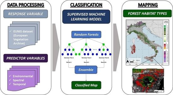
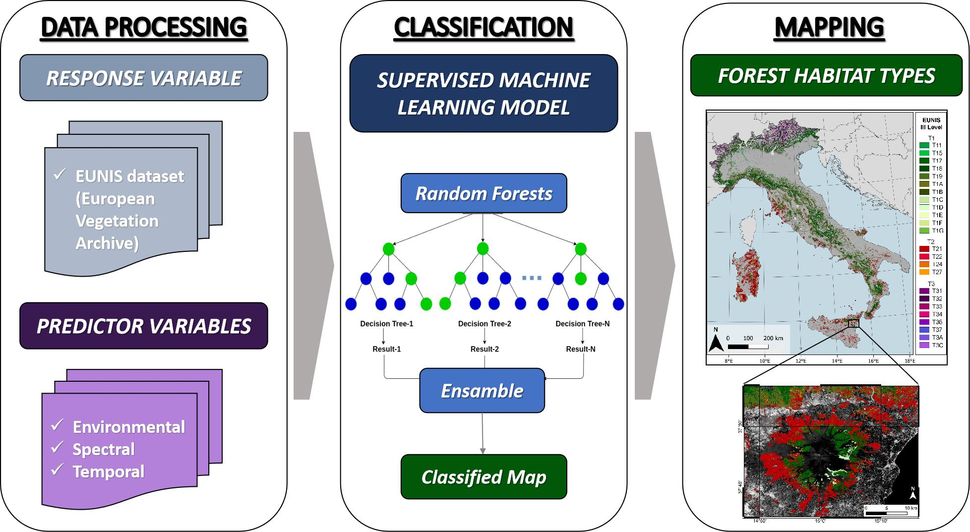
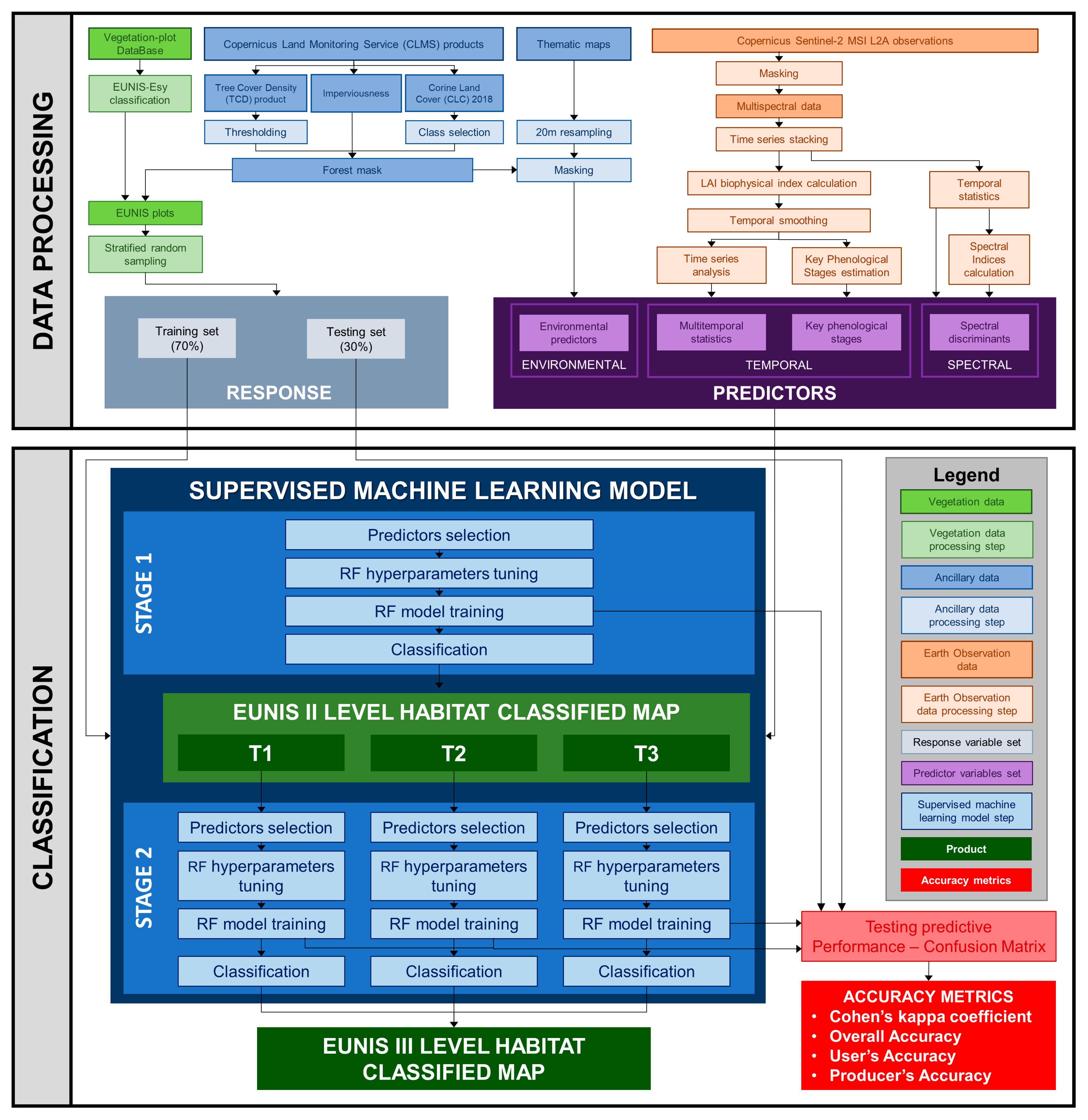
2.1. Research Step Flowchart
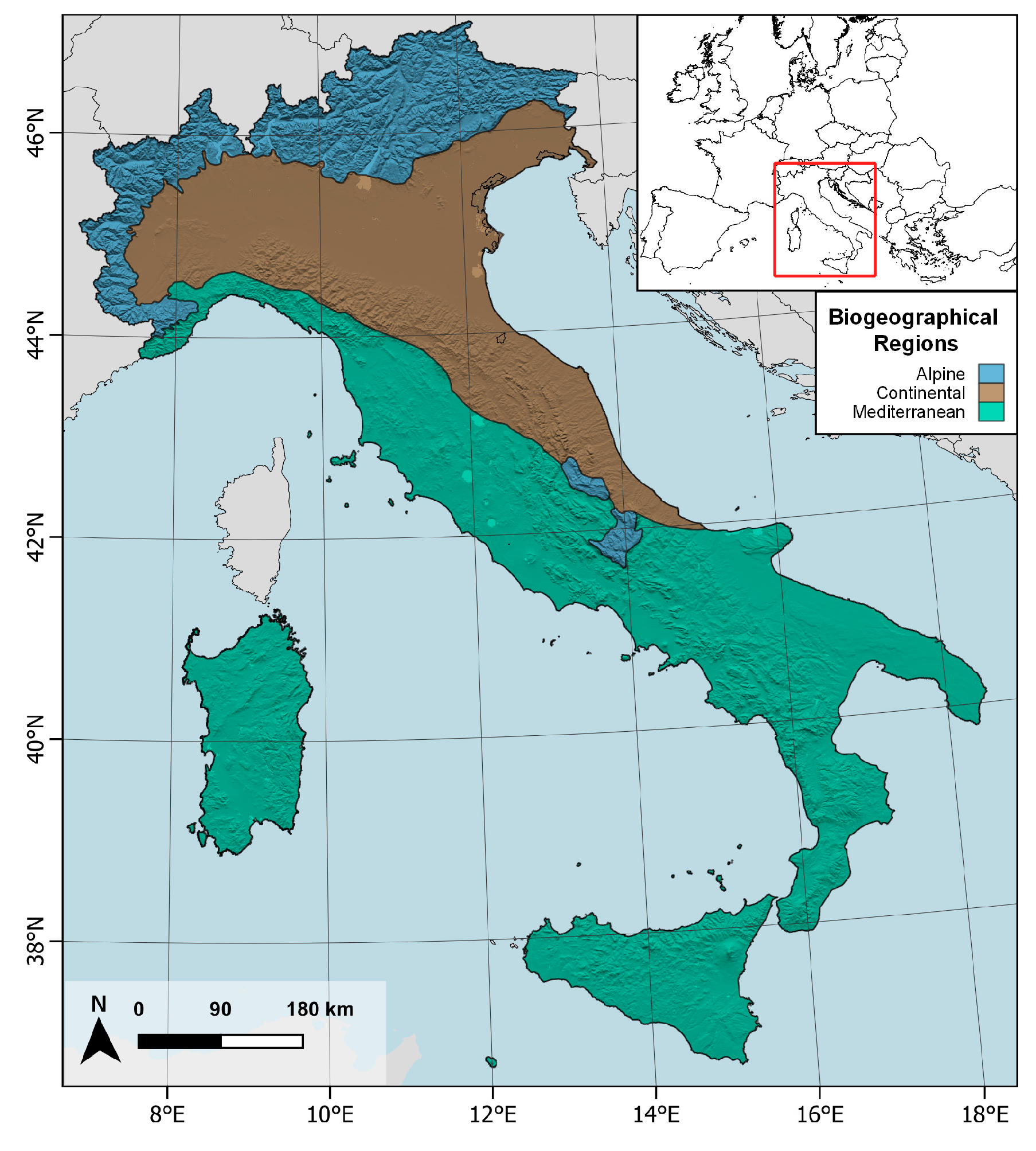
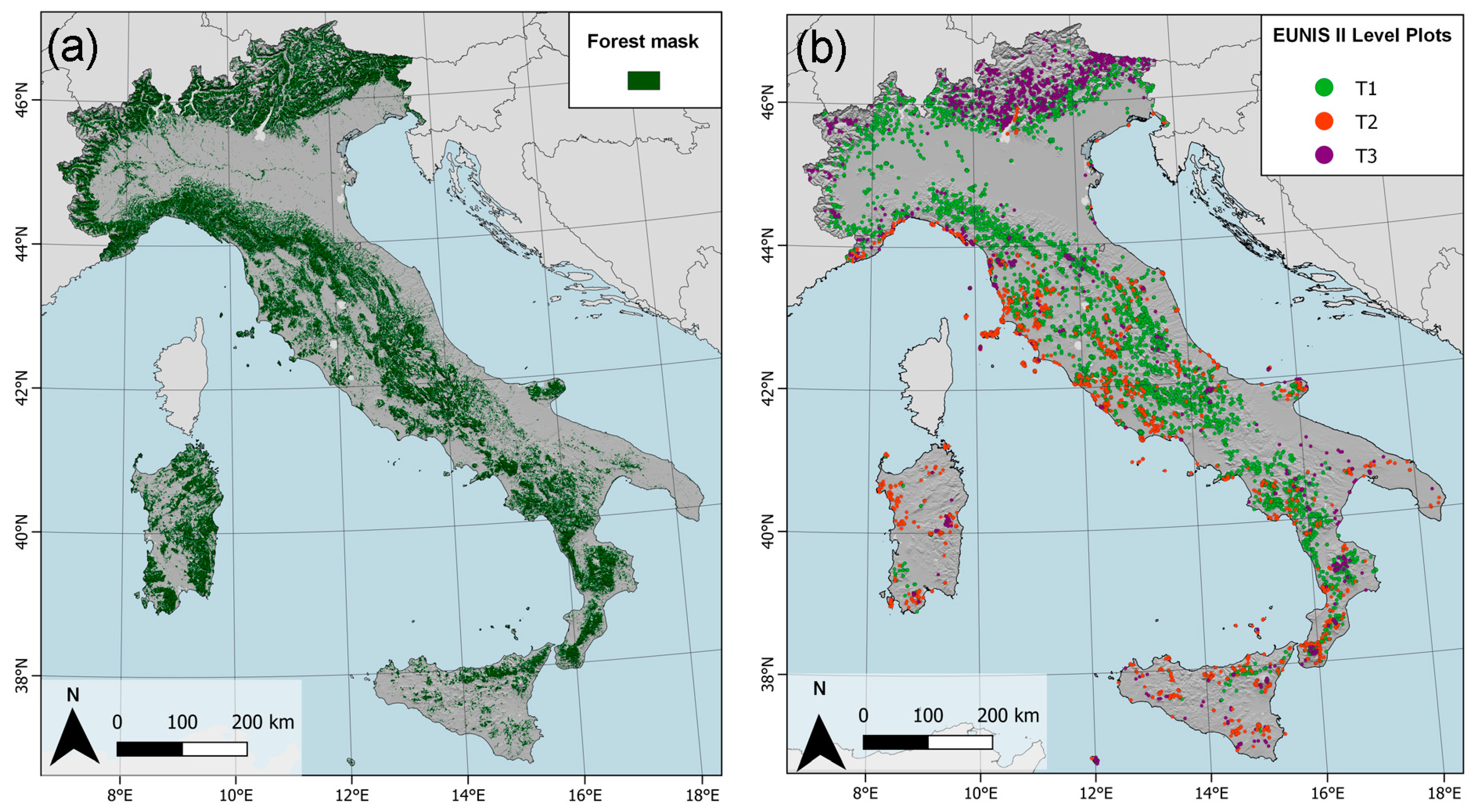
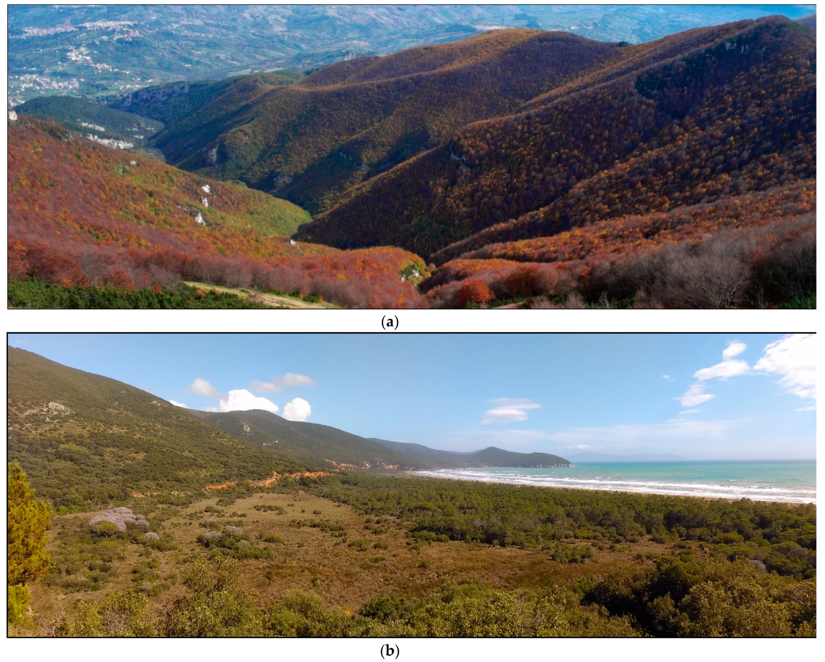
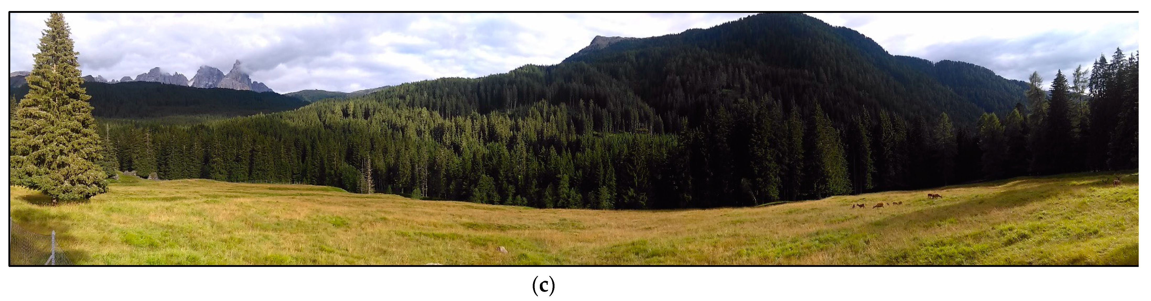
2.2. Study Area
2.3. Data Gathering and Processing
2.3.1. Response Variable
- resampling data: to perform the habitat classification only on the natural woodland areas, a forest mask was generated to resample the vegetation plots. The mask was obtained by combining Copernicus Land Monitoring Service products, specifically the High-Resolution Layers Tree Cover Density (TCD, [67]), the Imperviousness [68], and the CORINE Land Cover [69]. All of the records outside the forest mask were excluded;
- clustering data: from the whole dataset only forest habitats were extracted and clustered according to the EUNIS hierarchical classification nomenclature, following the EUNIS-ESy definitions [22]; and,
- filtering data: all data assigned at more than one EUNIS codes (e.g., bias plots assignment of mixed forest that linked at two different EUNIS groups) and all data recorded with the same geographic coordinates (i.e., plots of re-surveying monitoring research activities) were also excluded. Finally, a visualization data test was performed to identify spatial mismatches errors and/or spatial bias occurrences.
2.3.2. Predictor Variables
- environmental data: variables related to geographic, topographic, climatic, and soil properties;
- spectral data: variables extracted from EO satellite sensors; and,
- temporal data: variables representing temporal statistics and phenological metrics estimated from the biophysical index time series, generated from satellite EO data.
2.4. Classification
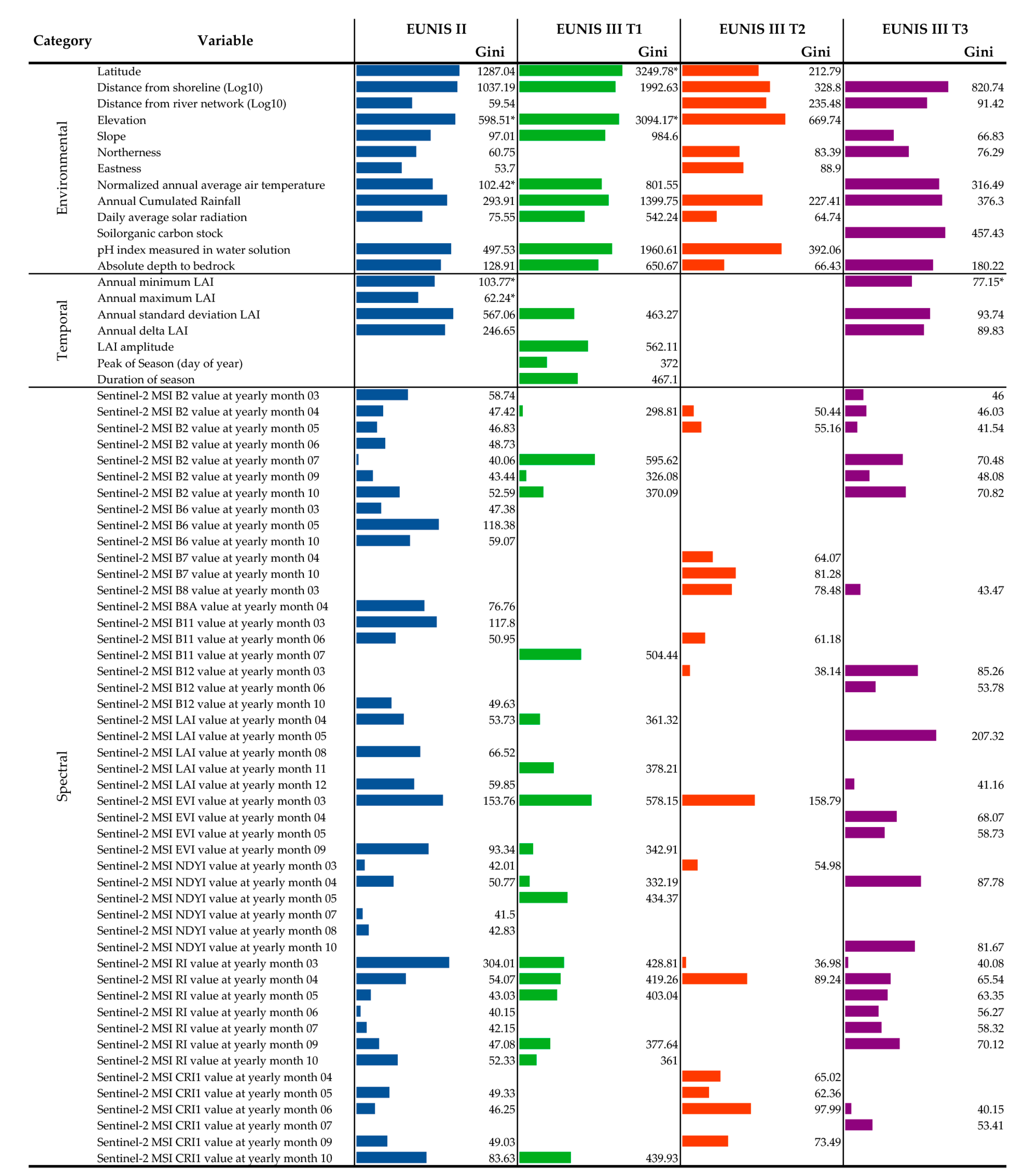
2.4.1. Predictors Selection
2.4.2. Supervised Machine Learning Model
3. Results
3.1. Response Variable
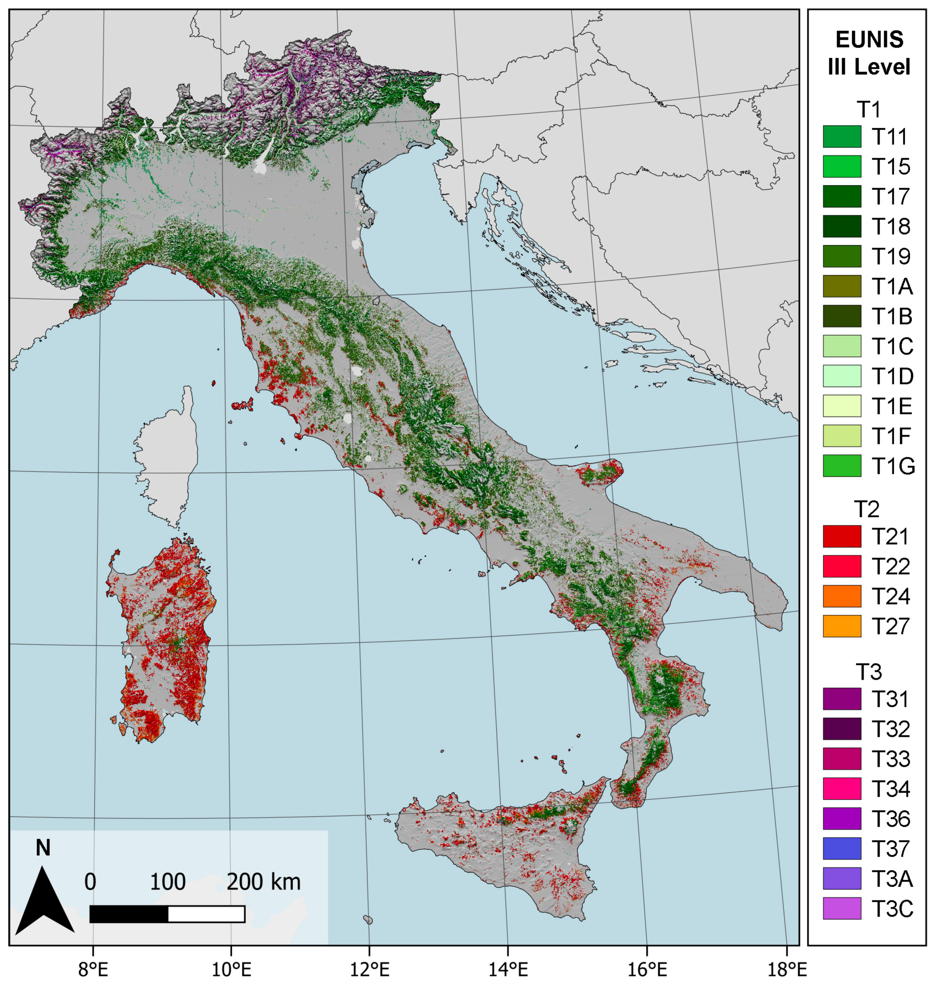
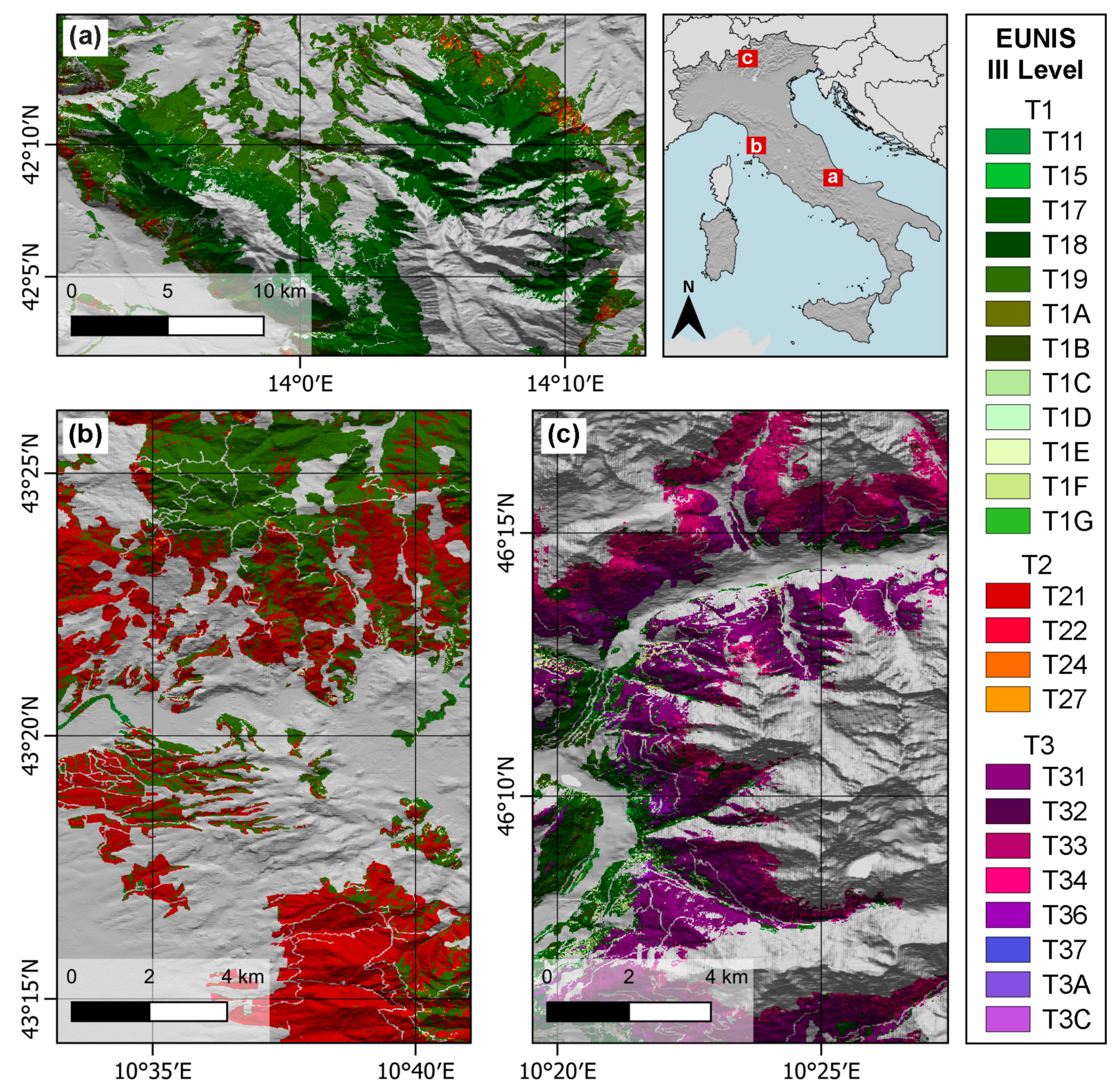
3.2. Classification
3.2.1. Predictor Variables and Selection
3.2.2. Supervised Machine Learning Model
4. Discussion
5. Conclusions
Author Contributions
Funding
Institutional Review Board Statement
Informed Consent Statement
Acknowledgments
Conflicts of Interest
Appendix A

| CATEGORY | SUBCATEGORY | NAME | DESCRIPTION | UNITS |
|---|---|---|---|---|
| Environmental | Geographic | Lat | Latitude 20 m cellcentroid | Degrees |
| dCoastLog | Distance from shoreline (Log10) | km | ||
| dRivLog | Distance from river network (Log10) | km | ||
| Geomorphologic | Elev | Elevation | m a.s.l. | |
| Slope | Slope | degrees | ||
| NorthN | Northerness | Polar units | ||
| EastN | Eastness | Polar units | ||
| Climatic | TannNorm | Normalized annual average air temperature | Celsius degrees | |
| CRFann | Annual Cumulated Rainfall | mm/year | ||
| sRad | Daily average solar radiation | WH/m2 | ||
| Soil properties | ORCDRC | Soil organic carbon stock | permille | |
| PHIHOX | pH index measured in water solution | pH | ||
| BDTICM | Absolute depth to bedrock | cm | ||
| Temporal | Temporal statistics | LAI_min | Annual minimum LAI | m2/m2 |
| LAI_avg | Annualaverage LAI | m2/m2 | ||
| LAI_max | Annual maximum LAI | m2/m2 | ||
| LAI_std | Annual standard deviation LAI | m2/m2 | ||
| LAI_delta | Annual delta LAI | m2/m2 | ||
| LAI_djf_min | Winter (December, January, February) minimum LAI | m2/m2 | ||
| LAI_djf_avg | Winter (December, January, February) average LAI | m2/m2 | ||
| LAI_djf_max | Winter (December, January, February) maximum LAI | m2/m2 | ||
| LAI_jja_avg | Summer (June, July, August) average LAI | m2/m2 | ||
| LAI_jja_max | Summer (June, July, August) maximum LAI | m2/m2 | ||
| Phenological metrics | SGS_doy | Start of Growing Season (DoY) | DoY | |
| SGS_value | Start of Growing Season LAI | m2/m2 | ||
| PoS_doy | Peak of Season (DoY) | DoY | ||
| PoS_value | Peak of Season LAI | m2/m2 | ||
| EGS_doy | End of Growing Season (DoY) | DoY | ||
| EGS_value | End of Growing Season VI | m2/m2 | ||
| EoS_doy | End of Season (DoY) | DoY | ||
| EoS_value | End of Season VI | m2/m2 | ||
| greenup_doy | Greenup (DoY) | DoY | ||
| greenup_rate | Greenup rate VI | m2/m2 | ||
| senescence_doy | Senescence (DoY) | DoY | ||
| senescence_rate | Senescence rate LAI | m2/m2 | ||
| amplitude | LAI amplitude | m2/m2 | ||
| DoS | Duration of season | Days | ||
| LMP | Length of Maturity Plateau | Days | ||
| STI | Seasonal time integrated LAI | m2/m2 | ||
| Spectral | Spectral data | B2_m03 | Sentinel-2 MSI B2 value at yearly month 03 | reflectance |
| B2_m04 | Sentinel-2 MSI B2 value at yearly month 04 | reflectance | ||
| B2_m05 | Sentinel-2 MSI B2 value at yearly month 05 | reflectance | ||
| B2_m06 | Sentinel-2 MSI B2 value at yearly month 06 | reflectance | ||
| B2_m07 | Sentinel-2 MSI B2 value at yearly month 07 | reflectance | ||
| B2_m08 | Sentinel-2 MSI B2 value at yearly month 08 | reflectance | ||
| B2_m09 | Sentinel-2 MSI B2 value at yearly month 09 | reflectance | ||
| B2_m10 | Sentinel-2 MSI B2 value at yearly month 10 | reflectance | ||
| B3_m03 | Sentinel-2 MSI B3 value at yearly month 03 | reflectance | ||
| B3_m04 | Sentinel-2 MSI B3 value at yearly month 04 | reflectance | ||
| B3_m05 | Sentinel-2 MSI B3 value at yearly month 05 | reflectance | ||
| B3_m06 | Sentinel-2 MSI B3 value at yearly month 06 | reflectance | ||
| B3_m07 | Sentinel-2 MSI B3 value at yearly month 07 | reflectance | ||
| B3_m08 | Sentinel-2 MSI B3 value at yearly month 08 | reflectance | ||
| B3_m09 | Sentinel-2 MSI B3 value at yearly month 09 | reflectance | ||
| B3_m10 | Sentinel-2 MSI B3 value at yearly month 10 | reflectance | ||
| B4_m03 | Sentinel-2 MSI B4 value at yearly month 03 | reflectance | ||
| B4_m04 | Sentinel-2 MSI B4 value at yearly month 04 | reflectance | ||
| B4_m05 | Sentinel-2 MSI B4 value at yearly month 05 | reflectance | ||
| B4_m06 | Sentinel-2 MSI B4 value at yearly month 06 | reflectance | ||
| B4_m07 | Sentinel-2 MSI B4 value at yearly month 07 | reflectance | ||
| B4_m08 | Sentinel-2 MSI B4 value at yearly month 08 | reflectance | ||
| B4_m09 | Sentinel-2 MSI B4 value at yearly month 09 | reflectance | ||
| B4_m10 | Sentinel-2 MSI B4 value at yearly month 10 | reflectance | ||
| B5_m03 | Sentinel-2 MSI B5 value at yearly month 03 | reflectance | ||
| B5_m04 | Sentinel-2 MSI B5 value at yearly month 04 | reflectance | ||
| B5_m05 | Sentinel-2 MSI B5 value at yearly month 05 | reflectance | ||
| B5_m06 | Sentinel-2 MSI B5 value at yearly month 06 | reflectance | ||
| B5_m07 | Sentinel-2 MSI B5 value at yearly month 07 | reflectance | ||
| B5_m08 | Sentinel-2 MSI B5 value at yearly month 08 | reflectance | ||
| B5_m09 | Sentinel-2 MSI B5 value at yearly month 09 | reflectance | ||
| B5_m10 | Sentinel-2 MSI B5 value at yearly month 10 | reflectance | ||
| B6_m03 | Sentinel-2 MSI B6 value at yearly month 03 | reflectance | ||
| B6_m04 | Sentinel-2 MSI B6 value at yearly month 04 | reflectance | ||
| B6_m05 | Sentinel-2 MSI B6 value at yearly month 05 | reflectance | ||
| B6_m06 | Sentinel-2 MSI B6 value at yearly month 06 | reflectance | ||
| B6_m07 | Sentinel-2 MSI B6 value at yearly month 07 | reflectance | ||
| B6_m08 | Sentinel-2 MSI B6 value at yearly month 08 | reflectance | ||
| B6_m09 | Sentinel-2 MSI B6 value at yearly month 09 | reflectance | ||
| B6_m10 | Sentinel-2 MSI B6 value at yearly month 10 | reflectance | ||
| B7_m03 | Sentinel-2 MSI B7 value at yearly month 03 | reflectance | ||
| B7_m04 | Sentinel-2 MSI B7 value at yearly month 04 | reflectance | ||
| B7_m05 | Sentinel-2 MSI B7 value at yearly month 05 | reflectance | ||
| B7_m06 | Sentinel-2 MSI B7 value at yearly month 06 | reflectance | ||
| B7_m07 | Sentinel-2 MSI B7 value at yearly month 07 | reflectance | ||
| B7_m08 | Sentinel-2 MSI B7 value at yearly month 08 | reflectance | ||
| B7_m09 | Sentinel-2 MSI B7 value at yearly month 09 | reflectance | ||
| B7_m10 | Sentinel-2 MSI B7 value at yearly month 10 | reflectance | ||
| B8_m03 | Sentinel-2 MSI B8 value at yearly month 03 | reflectance | ||
| B8_m04 | Sentinel-2 MSI B8 value at yearly month 04 | reflectance | ||
| B8_m05 | Sentinel-2 MSI B8 value at yearly month 05 | reflectance | ||
| B8_m06 | Sentinel-2 MSI B8 value at yearly month 06 | reflectance | ||
| B8_m07 | Sentinel-2 MSI B8 value at yearly month 07 | reflectance | ||
| B8_m08 | Sentinel-2 MSI B8 value at yearly month 08 | reflectance | ||
| B8_m09 | Sentinel-2 MSI B8 value at yearly month 09 | reflectance | ||
| B8_m10 | Sentinel-2 MSI B8 value at yearly month 10 | reflectance | ||
| B8A_m03 | Sentinel-2 MSI B8A value at yearly month 03 | reflectance | ||
| B8A_m04 | Sentinel-2 MSI B8A value at yearly month 04 | reflectance | ||
| B8A_m05 | Sentinel-2 MSI B8A value at yearly month 05 | reflectance | ||
| B8A_m06 | Sentinel-2 MSI B8A value at yearly month 06 | reflectance | ||
| B8A_m07 | Sentinel-2 MSI B8A value at yearly month 07 | reflectance | ||
| B8A_m08 | Sentinel-2 MSI B8A value at yearly month 08 | reflectance | ||
| B8A_m09 | Sentinel-2 MSI B8A value at yearly month 09 | reflectance | ||
| B8A_m10 | Sentinel-2 MSI B8A value at yearly month 10 | reflectance | ||
| B11_m03 | Sentinel-2 MSI B11 value at yearly month 03 | reflectance | ||
| B11_m04 | Sentinel-2 MSI B11 value at yearly month 04 | reflectance | ||
| B11_m05 | Sentinel-2 MSI B11 value at yearly month 05 | reflectance | ||
| B11_m06 | Sentinel-2 MSI B11 value at yearly month 06 | reflectance | ||
| B11_m07 | Sentinel-2 MSI B11 value at yearly month 07 | reflectance | ||
| B11_m08 | Sentinel-2 MSI B11 value at yearly month 08 | reflectance | ||
| B11_m09 | Sentinel-2 MSI B11 value at yearly month 09 | reflectance | ||
| B11_m10 | Sentinel-2 MSI B11 value at yearly month 10 | reflectance | ||
| B12_m03 | Sentinel-2 MSI B12 value at yearly month 03 | reflectance | ||
| B12_m04 | Sentinel-2 MSI B12 value at yearly month 04 | reflectance | ||
| B12_m05 | Sentinel-2 MSI B12 value at yearly month 05 | reflectance | ||
| B12_m06 | Sentinel-2 MSI B12 value at yearly month 06 | reflectance | ||
| B12_m07 | Sentinel-2 MSI B12 value at yearly month 07 | reflectance | ||
| B12_m08 | Sentinel-2 MSI B12 value at yearly month 08 | reflectance | ||
| B12_m09 | Sentinel-2 MSI B12 value at yearly month 09 | reflectance | ||
| B12_m10 | Sentinel-2 MSI B12 value at yearly month 10 | reflectance | ||
| Biophysical index | LAI_m01 | Sentinel-2 MSI LAI value at yearly month 01 | m2/m2 | |
| LAI_m02 | Sentinel-2 MSI LAI value at yearly month 02 | m2/m2 | ||
| LAI_m03 | Sentinel-2 MSI LAI value at yearly month 03 | m2/m2 | ||
| LAI_m04 | Sentinel-2 MSI LAI value at yearly month 04 | m2/m2 | ||
| LAI_m05 | Sentinel-2 MSI LAI value at yearly month 05 | m2/m2 | ||
| LAI_m06 | Sentinel-2 MSI LAI value at yearly month 06 | m2/m2 | ||
| LAI_m07 | Sentinel-2 MSI LAI value at yearly month 07 | m2/m2 | ||
| LAI_m08 | Sentinel-2 MSI LAI value at yearly month 08 | m2/m2 | ||
| LAI_m09 | Sentinel-2 MSI LAI value at yearly month 09 | m2/m2 | ||
| LAI_m10 | Sentinel-2 MSI LAI value at yearly month 10 | m2/m2 | ||
| LAI_m11 | Sentinel-2 MSI LAI value at yearly month 11 | m2/m2 | ||
| LAI_m12 | Sentinel-2 MSI LAI value at yearly month 12 | m2/m2 | ||
| EVI_m03 | Sentinel-2 MSI EVI value at yearly month 03 | dimensionless | ||
| EVI_m04 | Sentinel-2 MSI EVI value at yearly month 04 | dimensionless | ||
| EVI_m05 | Sentinel-2 MSI EVI value at yearly month 05 | dimensionless | ||
| EVI_m06 | Sentinel-2 MSI EVI value at yearly month 06 | dimensionless | ||
| EVI_m07 | Sentinel-2 MSI EVI value at yearly month 07 | dimensionless | ||
| EVI_m08 | Sentinel-2 MSI EVI value at yearly month 08 | dimensionless | ||
| EVI_m09 | Sentinel-2 MSI EVI value at yearly month 09 | dimensionless | ||
| EVI_m10 | Sentinel-2 MSI EVI value at yearly month 10 | dimensionless | ||
| NDYI_m03 | Sentinel-2 MSI NDYI value at yearly month 03 | dimensionless | ||
| NDYI_m04 | Sentinel-2 MSI NDYI value at yearly month 04 | dimensionless | ||
| NDYI_m05 | Sentinel-2 MSI NDYI value at yearly month 05 | dimensionless | ||
| NDYI_m06 | Sentinel-2 MSI NDYI value at yearly month 06 | dimensionless | ||
| NDYI_m07 | Sentinel-2 MSI NDYI value at yearly month 07 | dimensionless | ||
| NDYI_m08 | Sentinel-2 MSI NDYI value at yearly month 08 | dimensionless | ||
| NDYI_m09 | Sentinel-2 MSI NDYI value at yearly month 09 | dimensionless | ||
| NDYI_m10 | Sentinel-2 MSI NDYI value at yearly month 10 | dimensionless | ||
| RI_m03 | Sentinel-2 MSI RI value at yearly month 03 | dimensionless | ||
| RI_m04 | Sentinel-2 MSI RI value at yearly month 04 | dimensionless | ||
| RI_m05 | Sentinel-2 MSI RI value at yearly month 05 | dimensionless | ||
| RI_m06 | Sentinel-2 MSI RI value at yearly month 06 | dimensionless | ||
| RI_m07 | Sentinel-2 MSI RI value at yearly month 07 | dimensionless | ||
| RI_m08 | Sentinel-2 MSI RI value at yearly month 08 | dimensionless | ||
| RI_m09 | Sentinel-2 MSI RI value at yearly month 09 | dimensionless | ||
| RI_m10 | Sentinel-2 MSI RI value at yearly month 10 | dimensionless | ||
| CRI1_m03 | Sentinel-2 MSI CRI1 value at yearly month 03 | dimensionless | ||
| CRI1_m04 | Sentinel-2 MSI CRI1 value at yearly month 04 | dimensionless | ||
| CRI1_m05 | Sentinel-2 MSI CRI1 value at yearly month 05 | dimensionless | ||
| CRI1_m06 | Sentinel-2 MSI CRI1 value at yearly month 06 | dimensionless | ||
| CRI1_m07 | Sentinel-2 MSI CRI1 value at yearly month 07 | dimensionless | ||
| CRI1_m08 | Sentinel-2 MSI CRI1 value at yearly month 08 | dimensionless | ||
| CRI1_m09 | Sentinel-2 MSI CRI1 value at yearly month 09 | dimensionless | ||
| CRI1_m10 | Sentinel-2 MSI CRI1 value at yearly month 10 | dimensionless |
| Spectral Band | Band Name | S2A Central Wavelength (nm) | S2A Band Width (nm) | S2B Central Wavelength (nm) | S2B Band Width (nm) | Resolution (m) |
|---|---|---|---|---|---|---|
| B1 | Coastal aerosol | 443.9 | 27 | 442.3 | 45 | 60 |
| B2 | Blue | 496.6 | 98 | 492.1 | 98 | 10 |
| B3 | Green | 560.0 | 45 | 559.0 | 46 | 10 |
| B4 | Red | 664.5 | 38 | 665.0 | 39 | 10 |
| B5 | Red edge 1 | 703.9 | 19 | 703.8 | 20 | 20 |
| B6 | Red edge 2 | 740.2 | 18 | 739.1 | 18 | 20 |
| B7 | Red edge 3 | 782.5 | 28 | 779.7 | 28 | 20 |
| B8 | Near infrared | 835.1 | 145 | 833.0 | 133 | 10 |
| B8A | Near infrared narrow | 864.8 | 33 | 864.0 | 32 | 20 |
| B9 | Water vapor | 945.0 | 26 | 943.2 | 27 | 60 |
| B10 | SWIR Cirrus | 1373.5 | 75 | 1376.9 | 76 | 60 |
| B11 | Shortwave Infrared 1 | 1613.7 | 143 | 1610.4 | 141 | 20 |
| B12 | Shortwave Infrared 2 | 2202.4 | 242 | 2185.7 | 238 | 20 |
Appendix B


References
- Steffen, W.; Richardson, K.; Rockström, J.; Cornell, S.E.; Fetzer, I.; Bennett, E.M.; Biggs, R.; Carpenter, S.R.; de Vries, W.; de Wit, C.A.; et al. Planetary boundaries: Guiding human development on a changing planet. Science 2015, 347, 1259–1855. [Google Scholar] [CrossRef] [PubMed] [Green Version]
- Hooper, D.U.; Adair, E.C.; Cardinale, B.J.; Byrnes, J.E.; Hungate, B.A.; Matulich, K.L.; Gonzalez, A.; Duffy, J.E.; Gamfeldt, L.; O’Connor, M.I. A global synthesis reveals biodiversity loss as a major driver of ecosystem change. Nature 2012, 486, 105–108. [Google Scholar] [CrossRef] [PubMed]
- Theriault, J.; Young, L.; Barrett, L.F. The sense of should: A biologically-based framework for modeling social pressure. Phys. Life Rev. 2020. [Google Scholar] [CrossRef] [PubMed] [Green Version]
- Dryzek, J.S.; Norgaard, R.B.; Schlosberg, D. Climate change and society: Approaches and responses. In The Oxford Handbook of Climate Change and Society; Dryzek, J.S., Norgaard, R.B., Schlosberg, D., Eds.; Oxford University Press: Oxford, UK, 2011; pp. 3–17. [Google Scholar] [CrossRef]
- Hampton, S.E.; Strasser, C.A.; Tewksbury, J.J.; Gram, W.K.; Budden, A.E.; Batcheller, A.L.; Duke, C.S.; Porter, J.H. Big data and the future of ecology. Front. Ecol. Environ. 2013, 11, 156–162. [Google Scholar] [CrossRef] [Green Version]
- Runting, R.K.; Phinn, S.; Xie, Z.; Venter, O.; Watson, J.E. Opportunities for big data in conservation and sustainability. Nat. Commun. 2020, 11, 1–4. [Google Scholar] [CrossRef]
- Hallgren, W.; Beaumont, L.; Bowness, A.; Chambers, L.; Graham, E.; Holewa, H.; Laffan, S.; Mackey, B.; Nix, H.; Price, J.; et al. The biodiversity and climate change virtual laboratory: Where ecology meets big data. Environ. Model. Softw. 2016, 76, 182–186. [Google Scholar] [CrossRef] [Green Version]
- Palmer, M.A.; Bernhardt, E.S.; Chornesky, E.A.; Collins, S.L.; Dobson, A.P.; Duke, C.S.; Gold, B.D.; Jacobson, R.B.; Kingsland, S.E.; Kranz, R.H.; et al. Ecological science and sustainability for the 21st century. Front. Ecol. Environ. 2015, 3, 4–11. [Google Scholar] [CrossRef]
- Tuomisto, H. A consistent terminology for quantifying species diversity? Yes, it does exist. Oecologia 2010, 164, 853–860. [Google Scholar] [CrossRef]
- Convention on Biological Diversity. Available online: https://www.cbd.int/convention/text/ (accessed on 12 December 2020).
- Klijn, F.; Groen, C.L.G.; Witte, J.P.M. Ecoseries for potential site mapping, an example from the Netherlands. Landsc. Urban Plan. 1996, 35, 53–70. [Google Scholar] [CrossRef]
- Klijn, F. Ecosystem Classification for Environmental Management; Springer: Berlin/Heidelberg, Germany, 2013; Volume 2. [Google Scholar]
- Van der Maarel, E. Vegetation Ecology; Franklin, J., Ed.; John Wiley & Sons: Hoboken, NJ, USA, 2012. [Google Scholar]
- Janssen, J.A.M.; Rodwell, J.S.; García Criado, M.; Arts, G.; Bijlsma, R.J.; Schaminee, J.H.J. European Red List of Habitats: Part 2. In Terrestrial and Freshwater Habitats; Publications Office of the European Union: Luxembourg, 2016; ISBN 978-92-79-61588-7. [Google Scholar] [CrossRef]
- Bijlsma, R.J.; Agrillo, E.; Attorre, F.; Boitani, L.; Brunner, A.; Evans, P.; Foppen, R.; Gubbay, S.; Jansenn, J.A.M.; van Klaunen, A.; et al. Defining and Applying the Concept of Favourable Reference Values for Species Habitats under the EU Birds and Habitats Directives: Examples of Setting Favourable Reference Values; Report No. 2929; Wageningen Environmental Research: Wageningen, The Netherlands, 2018. [Google Scholar]
- Dengler, J.; Oldeland, J.; Jansen, F.; Chytry, M.; Ewald, J.; Finckh, M.; Glockler, F.; Lopez-Gonzalez, G.; Peet, R.K.; Schaminee, J.H.J. Vegetation databases for the 21st century. Biodivers. Ecol. 2012, 4, 15–24. [Google Scholar] [CrossRef] [Green Version]
- Chytrý, M.; Hennekens, S.M.; Jiménez-Alfaro, B.; Knollová, I.; Dengler, J.; Jansen, F.; Landucci, F.; Schaminée, J.H.; Acìc, S.; Agrillo, E.; et al. European Vegetation Archive (EVA): An integrated database of European vegetation plots. Appl. Veg. Sci. 2016, 19, 173–180. [Google Scholar] [CrossRef] [Green Version]
- Bruelheide, H.; Dengler, J.; Jiménez-Alfaro, B.; Purschke, O.; Hennekens, S.M.; Chytrý, M.; Pillar, V.D.; Jansen, F.; Kattge, J.; Sandel, B.; et al. sPlot–A new tool for global vegetation analyses. J. Veg. Sci. 2019, 30, 161–186. [Google Scholar] [CrossRef]
- Davies, C.E.; Moss, D. EUNIS Habitats Classification. In Final Report to the European Topic Centre on Nature Conservation; European Environment Agency: Copenhagen, Denmark, 1998. [Google Scholar]
- Davies, C.E.; Moss, D.; Hill, M.O. EUNIS Habitat Classification; European Environment Agency: Copenhagen, Denmark, 2004. [Google Scholar]
- EUNIS European Nature Information System. Available online: https://www.eea.europa.eu/data-and-maps/data/eunis-habitat-classification (accessed on 18 October 2020).
- Chytrý, M.; Tichý, L.; Hennekens, S.M.; Knollová, I.; Janssen, J.A.; Rodwell, J.S.; Peterka, T.; Marcenò, C.; Landucci, F.; Danihelka, J.; et al. EUNIS Habitat Classification: Expert system, characteristic species combinations and distribution maps of European habitats. Appl. Veg. Sci. 2020. [Google Scholar] [CrossRef]
- Revision of the EUNIS Habitat Classification. Available online: https://www.eea.europa.eu/themes/biodiversity/an-introduction-to-habitats/underpinning-european-policy-on-nature-conservation-1 (accessed on 15 November 2020).
- Guo, H.; Wang, L.; Liang, D. Big Earth Data from space: A new engine for Earth science. Sci. Bull. 2016, 61, 505–513. [Google Scholar] [CrossRef]
- Taramelli, A.; Tornato, A.; Magliozzi, M.L.; Mariani, S.; Valentini, E.; Zavagli, M.; Costantini, M.; Nieke, J.; Adams, J.; Rast, M. An Interaction Methodology to Collect and Assess User-Driven Requirements to Define Potential Opportunities of Future Hyperspectral Imaging Sentinel Mission. Remote Sens. 2020, 12, 1286. [Google Scholar] [CrossRef] [Green Version]
- Marvin, D.C.; Koh, L.P.; Lynam, A.J.; Wich, S.; Davies, A.B.; Krishnamurthy, R.; Stokes, E.; Starkey, R.; Asner, G.P. Integrating technologies for scalable ecology and conservation. Glob. Ecol. Cons. 2016, 7, 262–275. [Google Scholar] [CrossRef] [Green Version]
- Pettorelli, N.; Laurance, W.F.; O’Brien, T.G.; Wegmann, M.; Nagendra, H.; Turner, W. Satellite remote sensing for applied ecologists: Opportunities and challenges. J. Appl. Ecol. 2014, 51, 839–848. [Google Scholar] [CrossRef]
- Corbane, C.; Lang, S.; Pipkins, K.; Alleaume, S.; Deshayes, M.; Millán, V.E.G.; Strasser, T.; Borre, J.V.; Toon, S.; Michael, F. Remote sensing for mapping natural habitats and their conservation status–New opportunities and challenges. Int. J. Appl. Earth Obs. 2015, 37, 7–16. [Google Scholar] [CrossRef]
- Álvarez-Martínez, J.M.; Jiménez-Alfaro, B.; Barquín, J.; Ondiviela, B.; Recio, M.; Silió-Calzada, A.; Juanes, J.A. Modelling the area of occupancy of habitat types with remote sensing. Methods Ecol. Evol. 2018, 9, 580–593. [Google Scholar] [CrossRef]
- Wicaksono, P.; Aryaguna, P.A.; Lazuardi, W. Benthic habitat mapping model and cross validation using machine-learning classification algorithms. Remote Sens. 2019, 11, 1279. [Google Scholar] [CrossRef] [Green Version]
- Wang, R.; Gamon, J.A. Remote sensing of terrestrial plant biodiversity. Remote Sens. Environ. 2019, 231, 111218. [Google Scholar] [CrossRef]
- Adamo, M.; Tomaselli, V.; Tarantino, C.; Vicario, S.; Veronico, G.; Lucas, R.; Blonda, P. Knowledge-Based Classification of Grassland Ecosystem Based on Multi-Temporal WorldView-2 Data and FAO-LCCS Taxonomy. Remote Sens. 2020, 12, 1447. [Google Scholar] [CrossRef]
- Pesaresi, S.; Mancini, A.; Quattrini, G.; Casavecchia, S. Mapping Mediterranean Forest Plant Associations and Habitats with Functional Principal Component Analysis Using Landsat 8 NDVI Time Series. Remote Sens. 2020, 12, 1132. [Google Scholar] [CrossRef] [Green Version]
- Valentini, E.; Taramelli, A.; Filipponi, F.; Giulio, S. An effective procedure for EUNIS and Natura 2000 habitat type mapping in estuarine ecosystems integrating ecological knowledge and remote sensing analysis. Ocean Coast. Manag. 2015, 108, 52–64. [Google Scholar] [CrossRef]
- Valentini, E.; Taramelli, A.; Cappucci, S.; Filipponi, F.; Nguyen Xuan, A. Exploring the Dunes: The Correlations between Vegetation Cover Pattern and Morphology for Sediment Retention Assessment Using Airborne Multisensor Acquisition. Remote Sens. 2020, 12, 1229. [Google Scholar] [CrossRef] [Green Version]
- Marzialetti, F.; Giulio, S.; Malavasi, M.; Sperandii, M.G.; Acosta, A.T.R.; Carranza, M.L. Capturing Coastal Dune Natural Vegetation Types Using a Phenology-Based Mapping Approach: The Potential of Sentinel-2. Remote Sens. 2019, 11, 1506. [Google Scholar] [CrossRef] [Green Version]
- Spadoni, G.L.; Cavalli, A.; Congedo, L.; Munafò, M. Analysis of Normalized Difference Vegetation Index (NDVI) multi-temporal series for the production of forest cartography. Remote Sens. Appl. Soc. Environ. 2020, 20, 100419. [Google Scholar] [CrossRef]
- Rüetschi, M.; Schaepman, M.E.; Small, D. Using multitemporal sentinel-1 c-band backscatter to monitor phenology and classify deciduous and coniferous forests in northern switzerland. Remote Sens. 2018, 10, 55. [Google Scholar] [CrossRef] [Green Version]
- Rocchini, D.; Salvatori, N.; Beierkuhnlein, C.; Chiarucci, A.; de Boissieu, F.; Foerster, M.; Garzon-Lopez, C.X.; Gillespie, T.W.; Hauffe, H.C.; He, K.S.; et al. From local spectral species to global spectral communities: A benchmark for ecosystem diversity estimate by remote sensing. Ecol. Inform. 2020, 61, 101195. [Google Scholar] [CrossRef]
- Chytrý, M.; Schaminée, J.H.; Schwabe, A. Vegetation survey: A new focus for Applied Vegetation Science. Appl. Veg. Sci. 2011, 14. [Google Scholar] [CrossRef]
- EU Biodiversity Strategy for 2030. Available online: https://ec.europa.eu/environment/nature/biodiversity/strategy/index_en.htm (accessed on 12 December 2020).
- United Nations 2030 Agenda for Sustainable Development. Available online: https://sdgs.un.org/2030agenda (accessed on 23 November 2020).
- Berry, P.; Smith, A.; Eales, R.; Papadopoulou, L.; Erhard, M.; Meiner, A.; Bastrup-Birk, A.; Ivits, E.; Royo Gelabert, E.; Dige, G.; et al. Mapping and Assessing the Condition of Europe’s Ecosystems-Progress and Challenges, 3rd ed.; Publications Office of the European Union: Luxembourg, 2016; ISBN 978-92-79-55019-5. [Google Scholar] [CrossRef]
- Copernicus Land Monitoring System. Available online: https://land.copernicus.eu (accessed on 3 October 2020).
- Piedelobo, L.; Taramelli, A.; Schiavon, E.; Valentini, E.; Molina, J.-L.; Nguyen Xuan, A.; González-Aguilera, D. Assessment of Green Infrastructure in Riparian Zones Using Copernicus Programme. Remote Sens. 2019, 11, 2967. [Google Scholar] [CrossRef] [Green Version]
- Taramelli, A.; Lissoni, M.; Piedelobo, L.; Schiavon, E.; Valentini, E.; Nguyen Xuan, A.; González-Aguilera, D. Monitoring Green Infrastructure for Natural Water Retention Using Copernicus Global Land Products. Remote Sens. 2019, 11, 1583. [Google Scholar] [CrossRef] [Green Version]
- ESA—Sentinel Online. Available online: https://sentinel.esa.int/web/sentinel/home (accessed on 12 October 2020).
- Franklin, J. Moving beyond static species distribution models in support of conservation biogeography. Divers. Distrib. 2010, 16, 321–330. [Google Scholar] [CrossRef]
- Maggini, R.; Lehmann, A.; Zimmermann, N.E.; Guisan, A. Improving generalized regression analysis for the spatial prediction of forest communities. J. Biogeogr. 2006, 33, 1729–1749. [Google Scholar] [CrossRef]
- Miller, J.; Franklin, J. Modeling the distribution of four vegetation alliances using generalized linear models and classification trees with spatial dependence. Ecol. Model. 2002, 157, 227–247. [Google Scholar] [CrossRef]
- Engler, R.; Waser, L.T.; Zimmermann, N.E.; Schaub, M.; Berdos, S.; Ginzler, C.; Psomas, A. Combining ensemble modeling and remote sensing for mapping individual tree species at high spatial resolution. For. Ecol. Manag. 2013, 310, 64–73. [Google Scholar] [CrossRef]
- Kattenborn, T.; Lopatin, J.; Förster, M.; Braun, A.C.; Fassnacht, F.E. UAV data as alternative to field sampling to map woody invasive species based on combined Sentinel-1 and Sentinel-2 data. Remote Sens. Environ. 2019, 227, 61–73. [Google Scholar] [CrossRef]
- Vila-Viçosa, C.; Arenas-Castro, S.; Marcos, B.; Honrado, J.; García, C.; Vázquez, F.M.; Almeida, R.; Gonçalves, J. Combining Satellite Remote Sensing and Climate Data in Species Distribution Models to Improve the Conservation of Iberian White Oaks (Quercus L.). ISPRS Int. J. Geo-Inf. 2020, 9, 735. [Google Scholar] [CrossRef]
- Gavish, Y.; O’Connell, J.; Marsh, C.J.; Tarantino, C.; Blonda, P.; Tomaselli, V.; Kunin, W.E. Comparing the performance of flat and hierarchical Habitat/Land-Cover classification models in a NATURA 2000 site. ISPRS J. Photogramm. 2018, 136, 1–12. [Google Scholar] [CrossRef]
- Immitzer, M.; Neuwirth, M.; Böck, S.; Brenner, H.; Vuolo, F.; Atzberger, C. Optimal Input Features for Tree Species Classification in Central Europe Based on Multi-Temporal Sentinel-2 Data. Remote Sens. 2019, 11, 2599. [Google Scholar] [CrossRef] [Green Version]
- Compendium of EO Contributions to the SDGs Just Released. Available online: https://eo4society.esa.int/2021/01/15/compendium-of-eo-contributions-to-the-sdgs-just-released/ (accessed on 29 December 2020).
- Guisan, A.; Zimmermann, N.E. Predictive habitat distribution models in ecology. Ecol. Model. 2000, 135, 147–186. [Google Scholar] [CrossRef]
- Guisan, A.; Thuiller, W.; Zimmermann, N.E. Habitat Suitability and Distribution Models: With Applications in R; Cambridge University Press: Cambridge, UK, 2017; ISBN 987-0521765138. [Google Scholar]
- Marchetti, M.; Soldati, M.; Vandelli, V. The great diversity of Italian landscapes and landforms: Their origin and human imprint. In Landscapes and landforms of Italy; Springer: Berlin/Heidelberg, Germany, 2017; pp. 7–20. [Google Scholar]
- Fratianni, S.; Acquaotta, F. The climate of Italy. In Landscapes and Landforms of Italy; Springer: Berlin/Heidelberg, Germany, 2017; pp. 29–38. [Google Scholar]
- Land Use of Italy. Available online: https://www.isprambiente.gov.it/it/pubblicazioni/rapporti/territorio.-processi-e-trasformazioni-in-italia (accessed on 18 October 2020).
- Gasparini, P.; Di Cosmo, L. National Forest Inventory Reports—Italy. In National Forest Inventories—Assessment of Wood Availability and Use, 1st ed.; Vidal, C., Alberdi, I., Hernandez, L., Redmond, J., Eds.; Springer: Berlin/Heidelberg, Germany, 2016; pp. 485–506. ISBN 978-3-319-44014-9. [Google Scholar]
- Pividori, M.; Giannetti, F.; Barbati, A.; Chirici, G. European Forest Types: Tree species matrix. In European Atlas of Forest Tree Species; San-Miguel-Ayanz, J., de Rigo, D., Caudullo, G., Houston Durrant, T., Mauri, A., Eds.; Publications Office of the European Union: Luxembourg, 2016; p. e01f162. [Google Scholar]
- Cervellini, M.; Zannini, P.; Di Musciano, M.; Fattorini, S.; Jiménez-Alfaro, B.; Rocchini, D.; Field, R.; Vetaas, O.R.; Irl, S.D.H.; Beierkuhnlein, C.; et al. A grid-based map for the Biogeographical Regions of Europe. Biodivers. Data J. 2020, 8. [Google Scholar] [CrossRef] [PubMed]
- Europe Biogeographical Regions. Available online: https://www.eea.europa.eu/data-and-maps/data/biogeographical-regions-europe-3 (accessed on 3 September 2020).
- Agrillo, E.; Alessi, N.; Massimi, M.; Spada, F.; De Sanctis, M.; Francesconi, F.; Cambria, V.E.; Attorre, F. Nationwide Vegetation Plot Database–Sapienza University of Rome: State of the art, basic figures and future perspectives. Phytocoenologia 2017, 47, 221–222. [Google Scholar] [CrossRef]
- Tree Cover Density Layer. Available online: https://land.copernicus.eu/pan-european/high-resolution-layers/forests/tree-cover-density (accessed on 15 October 2020).
- Imperviousness Layer. Available online: https://land.copernicus.eu/pan-european/high-resolution-layers/imperviousness (accessed on 15 October 2020).
- Corine Land Cover 2018 Layer. Available online: http://groupware.sinanet.isprambiente.it/uso-copertura-e-consumo-di-suolo/library/copertura-del-suolo/corine-land-cover/corine-land-cover-2018-iv-livello (accessed on 15 October 2020).
- Descombes, P.; Walthert, L.; Baltensweiler, A.; Meuli, R.G.; Karger, D.N.; Ginzler, C.; Ginzler, G.; Zimmermann, N.E. Spatial modelling of ecological indicator values improves predictions of plant distributions in complex landscapes. Ecography 2020, 43, 1448–1463. [Google Scholar] [CrossRef]
- Italian Shoreline and River Network. Available online: http://www.pcn.minambiente.it/mattm/servizio-di-scaricamento-wfs/ (accessed on 22 October 2020).
- Digital Elevation Model of Italy at 20 m Spatial Resolution. Available online: http://www.sinanet.isprambiente.it/it/sia-ispra/download-mais/dem20/view (accessed on 22 October 2020).
- Braca, G.; Ducci, D. Development of a GIS based procedure (BIGBANG 1.0) for evaluating groundwater balances at National scale and comparison with groundwater resources evaluation at local scale. In Groundwater and Global Change in the Western Mediterranean Area; Springer: Berlin/Heidelberg, Germany, 2018; pp. 53–61. [Google Scholar]
- Fioravanti, G.; Toreti, A.; Fraschetti, P.; Perconti, W.; Desiato, F. Gridded monthly temperatures over Italy. In Proceedings of the 10th EMS Annual Meeting, Zürich, Switzerland, 13–17 September 2010; p. EMS2010-306. [Google Scholar]
- US Standard Atmosphere. 1976. Available online: https://ntrs.nasa.gov/citations/19770009539 (accessed on 24 November 2020).
- Súri, M.; Hofierka, J. A new GIS-based solar radiation model and its application tophotovoltaic assessments. Trans. GIS 2004, 8, 175–190. [Google Scholar] [CrossRef]
- Duveiller, G.; Filipponi, F.; Ceglar, A.; Bojanowski, J.; Alkama, R.; Stengel, M.; Cescatti, A. Widespread cloud enhancement adds further value to the world’s forests. Nat. Commun. 2020. submitted. [Google Scholar]
- Karsten, F.; Czeplak, G. Solar terrestial radiation dependent on the amount and type of clouds. Sol. Energy 1980, 24, 177–189. [Google Scholar] [CrossRef]
- Hagolle, O.; Huc, M.; Desjardins, C.; Auer, S.; Richter, R. MAJA Algorithm Theoretical Basis Document. Available online: https://0-doi-org.brum.beds.ac.uk/10.5281/zenodo.1209633 (accessed on 7 December 2017).
- Rouquié, B.; Hagolle, O.; Bréon, F.M.; Boucher, O.; Desjardins, C.; Rémy, S. Using Copernicus atmosphere monitoring service products to constrain the aerosol type in the atmospheric correction processor MAJA. Remote Sens. 2017, 9, 1230. [Google Scholar] [CrossRef] [Green Version]
- Croft, H.; Chen, J.M. Leaf pigment content. In Reference Module in Earth Systems and Environ-Mental Sciences; Elsevier: Amsterdam, The Netherlands, 2017; pp. 1–22. [Google Scholar]
- Huete, A.; Justice, C.; Liu, H. Development of vegetation and soil indices for MODIS-EOS. Remote Sens. Environ. 1994, 49, 224–234. [Google Scholar] [CrossRef]
- D’Andrimont, R.; Taymans, M.; Lemoine, G.; Ceglar, A.; Yordanov, M.; van der Velde, M. Detecting flowering phenology in oil seed rape parcels with Sentinel-1 and-2 time series. Remote Sens. Environ. 2020, 239, 111660. [Google Scholar] [CrossRef]
- Escadafal, R.; Huete, A. Improvement in remote sensing of low vegetation cover in arid regions by correcting vegetation indices for soil’noise’ (Etude des proprieties spectrales des sols arides appliquee a l’amelioration des indices de vegetation obtenus par teledetection). Acad. Sci. Comptes Rendus Ser. II Mec. Phys. Chim. Sci. Terre l’Univers 1991, 312, 1385–1391. [Google Scholar]
- Gitelson, A.A.; Zur, Y.; Chivkunova, O.B.; Merzlyak, M.N. Assessing Carotenoid Content in Plant Leaves with Reflectance Spectroscopy. Photochem. Photobiol. 2002, 75, 272–281. [Google Scholar] [CrossRef]
- Weiss, M.; Baret, F. S2 ToolBox Level 2 Products: LAI, FAPAR, FCOVER. 2016. Available online: https://step.esa.int/docs/extra/ATBD_S2ToolBox_L2B_V1.1.pdf (accessed on 31 March 2019).
- Filipponi, F. Exploitation of Sentinel-2 Time Series to Map Burned Areas at the National Level: A Case Study on the 2017 Italy Wildfires. Remote. Sens. 2019, 11, 622. [Google Scholar] [CrossRef] [Green Version]
- Filipponi, F.; Smiraglia, D.; Agrillo, E. Earth Observation for Phenological Metrics (EO4PM): Temporal discriminant to characterize forest ecosystems. Remote Sens. (manuscript in preparation).
- Gu, L.; Post, W.; Baldocchi, D.; Black, T.; Suyker, A.; Verma, S.; Vesala, T.; Wofsy, S. Characterizing the seasonal dynamics of plant community photosynthesis across a range of vegetation types. In Phenology of Ecosystem Processes; Noormets, A., Ed.; Springer: Berlin/Heidelberg, Germany, 2009; pp. 35–58. ISBN 978-1-4419-0026-5 2. [Google Scholar]
- Pesaresi, S.; Mancini, A.; Casavecchia, S. Recognition and Characterization of Forest Plant Communities through Remote-Sensing NDVI Time Series. Diversity 2020, 12, 313. [Google Scholar] [CrossRef]
- Zuur, A.F.; Ieno, E.N.; Elphick, C.S. A protocol for data exploration to avoid common statistical problems. Methods Ecol. Evol. 2010, 1, 3–14. [Google Scholar] [CrossRef]
- Kursa, M.B.; Rudnicki, W.R. Feature selection with the Boruta package. J. Stat. Softw. 2010, 36, 1–13. [Google Scholar] [CrossRef] [Green Version]
- Breiman, L. Random forests. Mach. Learn. 2001, 45, 5–32. [Google Scholar] [CrossRef] [Green Version]
- Wright, M.N.; Ziegler, A. Ranger: A Fast Implementation of Random Forests for High Dimensional Data in C++ and R. J. Stat. Softw. 2017, 77, 1–17. [Google Scholar] [CrossRef] [Green Version]
- Attorre, F.; Cambria, V.E.; Agrillo, E.; Alessi, N.; Alfò, M.; De Sanctis, M.; Malatesta, M.; Sitzia, T.; Guarino, R.; Marcenò, C.; et al. Finite Mixture Model-based classification of a complex vegetation system. Veg. Class. Sur. 2020, 1, 77. [Google Scholar] [CrossRef]
- Chirici, G.; Giannetti, F.; McRoberts, R.E.; Travaglini, D.; Pecchi, M.; Maselli, F.; Chiesi, M.; Corona, P. Wall-to-wall spatial prediction of growing stock volume based on Italian National Forest Inventory plots and remotely sensed data. Int. J. Appl. Earth Obs. 2020, 84, 101959. [Google Scholar] [CrossRef]
- Genuer, R.; Poggi, J.M.; Tuleau-Malot, C.; Villa-Vialaneix, N. Random forests for big data. Big Data Res. 2017, 9, 28–46. [Google Scholar] [CrossRef]
- Lapini, A.; Pettinato, S.; Santi, E.; Paloscia, S.; Fontanelli, G.; Garzelli, A. Comparison of Machine Learning Methods Applied to SAR Images for Forest Classification in Mediterranean Areas. Remote Sens. 2020, 12, 369. [Google Scholar] [CrossRef] [Green Version]
- Probst, P.; Wright, M.N.; Boulesteix, A.L. Hyperparameters and tuning strategies for random forest. Wires Data Min. Knowl. 2019, 9. [Google Scholar] [CrossRef] [Green Version]
- Bischl, B.; Lang, M.; Kotthoff, L.; Schiffner, J.; Richter, J.; Studerus, E.; Casalicchio, G.; Jones, Z.M. mlr: Machine Learning in R. J. Mach. Learn. Res. 2016, 17, 1–5. [Google Scholar] [CrossRef]
- Stehman, S.V.; Foody, G.M. Key issues in rigorous accuracy assessment of land cover products. Remote Sens. Environ. 2019, 231, 111199. [Google Scholar] [CrossRef]
- Pedrotti, F. Plant and Vegetation Mapping; Springer Science & Business Media: Berlin/Heidelberg, Germany, 2012. [Google Scholar]
- Pignatti, S.; Cavalli, R.M.; Cuomo, V.; Fusilli, L.; Pascucci, S.; Poscolieri, M.; Santini, F. Evaluating Hyperion capability for land cover mapping in a fragmented ecosystem: Pollino National Park, Italy. Remote Sens. Environ. 2009, 113, 622–634. [Google Scholar] [CrossRef]
- Wegmann, M.; Leutner, B.; Dech, S. Remote Sensing and GIS for Ecologists: Using Open Source Software; Pelagic Publishing Ltd.: Exeter, UK, 2016. [Google Scholar]
- Valerio, F.; Ferreira, E.; Godinho, S.; Pita, R.; Mira, A.; Fernandes, N.; Santos, S.M. Predicting Microhabitat Suitability for an Endangered Small Mammal Using Sentinel-2 Data. Remote Sens. 2020, 12, 562. [Google Scholar] [CrossRef] [Green Version]
- Steinacker, C.; Beierkuhnlein, C.; Jaeschke, A. Assessing the exposure of forest habitat types to projected climate change—Implications for Bavarian protected areas. Ecol. Evol. 2019, 9, 14417–14429. [Google Scholar] [CrossRef] [PubMed]
- Wang, Q.; Adiku, S.; Tenhunen, J.; Granier, A. On the relationship of NDVI with leaf area index in a deciduous forest site. Remote Sens. Environ. 2005, 94, 244–255. [Google Scholar] [CrossRef]
- Zimmermann, N.E.; Edwards, T.C., Jr.; Moisen, G.G.; Frescino, T.S.; Blackard, J.A. Remote sensing-based predictors improve distribution models of rare, early successional and broadleaf tree species in Utah. J. Appl. Ecol. 2007, 44, 1057–1067. [Google Scholar] [CrossRef] [PubMed] [Green Version]
- Večeřa, M.; Divíšek, J.; Lenoir, J.; Jiménez-Alfaro, B.; Biurrun, I.; Knollová, I.; Agrillo, E.; Campos, J.A.; Carni, A.; Jimènez, G.C.; et al. Alpha diversity of vascular plants in European forests. J. Biogeogr. 2019, 46, 1919–1935. [Google Scholar] [CrossRef]
- Pesaresi, S.; Galdenzi, D.; Biondi, E.; Casavecchia, S. Bioclimate of Italy: Application of the worldwide bioclimatic classification system. J. Maps 2014, 10, 538–553. [Google Scholar] [CrossRef]
- Saha, A.K.; Arora, M.K.; Csaplovics, E.; Gupta, R.P. Land cover classification using IRS LISS III image and DEM in a rugged terrain: A case study in Himalayas. Geocarto Int. 2005, 20, 33–40. [Google Scholar] [CrossRef]
- Piussi, P.; Pettenella, D. Spontaneous afforestation of fallows in Italy. NEWFOR 2000, 151, 151–163. [Google Scholar]
- Giacomini, V.; Fenaroli, L. Conosci l’Italia. Volume 2. La Flora; Touring Club Italiano: Milano, Italy, 1958. [Google Scholar]
- Pignatti, S. I Boschi d’Italia. Sinecologia e Biodiversità; Utet: Turin, Italy, 1998. [Google Scholar]
- Rocchini, D.; Hortal, J.; Lengyel, S.; Lobo, J.M.; Jimenez-Valverde, A.; Ricotta, C.; Bacaro, G.; Chiarucci, A. Accounting for uncertainty when mapping species distributions: The need for maps of ignorance. Progr. Phys. Geog. 2011, 35, 211–226. [Google Scholar] [CrossRef]
- Chiarucci, A. To sample or not to sample? That is the question for the vegetation scientist. Folia Geobot. 2007, 42, 209. [Google Scholar] [CrossRef]
- Fattorini, L.; Marcheselli, M.; Pisani, C. A three-phase sampling strategy for large-scale multi-resource forest inventories. J. Agric. Biol. Environ. Stat. 2006, 11, 296. [Google Scholar] [CrossRef]
- Abrams, J.F.; Vashishtha, A.; Wong, S.T.; Nguyen, A.; Mohamed, A.; Wieser, S.; Kuijper, A.; Wilting, A.; Mukhopadhyay, A. Habitat-Net: Segmentation of habitat images using deep learning. Ecol. Inform. 2019, 51, 121–128. [Google Scholar] [CrossRef]
- Chen, W.; Zheng, Q.; Xiang, H.; Chen, X.; Sakai, T. Forest Canopy Height Estimation Using Polarimetric Interferometric Synthetic Aperture Radar (PolInSAR) Technology Based on Full-Polarized ALOS/PALSAR Data. Remote Sens. 2021, 13, 174. [Google Scholar] [CrossRef]


| FOREST TYPE | DOMINANT SPECIES |
|---|---|
| Hemiboreal forest and nemoral coniferous and mixed broadleaved coniferous forest | Picea abies (Norway spruce), Pinus pinaster (Maritime pine), Pinus sylvestris (Scots pine) and Pinus nigra (Black pine) |
| Alpine coniferous forest | P. abies, Larix decidua (European larch), Pinus mugo (Bog pine), Pinus cembra (Swiss pine) and Abies alba (European silver fir) |
| Coniferous forests of the Mediterranean, Anatolian and Macaronesian regions | P. pinaster, Pinus halepensis (Aleppo pine), Pinus pinea (Stone pine), Pinus heldeeicrii (Bosnian pine) |
| Mesophytic deciduous forest | Carpinus betulus (Common hornbeam) |
| Mountainous beech forest | Fagus sylvatica (Europe beech) and A. alba (European silver fir) |
| Thermophilus deciduous forest | Deciduous Oaks, Tilia spp. (little leaf linden), Ostrya carpinifolia (European hop-hornbeam) and Castanea sativa (sweet chestnut) |
| Broadleaved evergreen forest | Quercus ilex (evergreen oak) and Quercus suber (cork oak) |
| Floodplain forest | Salix spp (Willow), Populus spp. (Poplar) and Alnus glutinosa, (Common alder) |
| Not riverine alder, birch, or aspen forest | Alnus cordata (Italian alder) |
| Spectral Index | Equation | Reference |
|---|---|---|
| Enhanced Vegetation Index EVI | [82] | |
| Normalized Difference Yellow Index NDYI | [83] | |
| Normalized Difference Red/Green Redness Index RI | [84] | |
| Carotenoid Reflectance Index CRI1 | [85] |
| EUNIS Code II Level | EUNIS Code III Level | EUNIS 2020 Habitat Name | Records |
|---|---|---|---|
| T1 | Broadleaved Deciduous forest habitat-type | 8328 | |
| T11 | Temperate Salix and Populus riparian forest | 1027 | |
| T15 | Broadleaved swamp forest on non-acid peat | 772 | |
| T17 | Fagus forest on non-acid soils | 2404 | |
| T18 | Fagus forest on acid soils | 614 | |
| T19 | Temperate and sub-mediterranean thermophilous deciduous forest | 1389 | |
| T1A | Mediterranean thermophilous deciduous forest | 815 | |
| T1B | Acidophilous Quercus forest | 147 | |
| T1C | Temperate and boreal mountain Betula and P. tremula forest on mineral soils | 32 | |
| T1D | Southern European mountain Betula and P. tremula forest on mineral soils | 36 | |
| T1E | Carpinus and Quercus mesic deciduous forest | 260 | |
| T1F | Ravine forest | 541 | |
| T1G | A. cordata forest | 291 | |
| T2 | Broadleaved Evergreen forest habitat-type | 3776 | |
| T21 | Mediterranean evergreen Quercus forest | 3015 | |
| T22 | Mainland laurophyllous forest | 145 | |
| T24 | Olea europaea and Ceratonia siliqua forest | 492 | |
| T27 | Ilex aquifolium forest | 124 | |
| T3 | Needleleaved forest habitat-type | 2281 | |
| T31 | Temperate mountain Picea forest | 412 | |
| T32 | Temperate mountain Abies forest | 500 | |
| T33 | Mediterranean mountain Abies forest | 98 | |
| T34 | Temperate subalpine Larix, P. cembra and P. uncinata forest | 461 | |
| T36 | Temperate and sub-mediterranean montane P. sylvestris–P. nigra forest | 295 | |
| T37 | Mediterranean montane P. sylvestris–P. nigra forest | 84 | |
| T3A | Mediterranean lowland to submontane Pinus forest | 365 | |
| T3C | Taxus baccata forest | 63 |
| Map Class | Reference Class | ||||
|---|---|---|---|---|---|
| T1 | T2 | T3 | Sum | UA (SE) | |
| T1 | 1037 | 80 | 63 | 1180 | 89.9 (0.00) |
| T2 | 93 | 564 | 0 | 657 | 87.6 (0.01) |
| T3 | 23 | 0 | 162 | 185 | 72 (0.02) |
| Sum | 1153 | 644 | 225 | OA (SE) 87.2% (0.75) | |
| PA (SE) | 87.9 (0.00) | 85.8 (0.03) | 87.6 (0.13) | Kappa 0.77 | |
| Map Class | Reference Class | |||||||||||||
|---|---|---|---|---|---|---|---|---|---|---|---|---|---|---|
| T11 | T15 | T17 | T18 | T19 | T1A | T1B | T1C | T1D | T1E | T1F | T1G | Sum | UA (SE) | |
| T11 | 36 | 4 | 1 | 1 | 6 | 1 | 4 | 0 | 0 | 2 | 2 | 0 | 57 | 50.7 (0.06) |
| T15 | 5 | 22 | 1 | 2 | 0 | 1 | 0 | 0 | 0 | 0 | 0 | 0 | 31 | 55 (0.08) |
| T17 | 6 | 3 | 357 | 22 | 27 | 2 | 5 | 3 | 0 | 0 | 20 | 4 | 449 | 85.6 (0.02) |
| T18 | 1 | 0 | 16 | 17 | 0 | 0 | 1 | 1 | 0 | 1 | 1 | 0 | 38 | 37.8 (0.08) |
| T19 | 13 | 6 | 20 | 0 | 206 | 54 | 2 | 0 | 3 | 17 | 8 | 6 | 335 | 73.3 (0.03) |
| T1A | 6 | 0 | 3 | 0 | 30 | 87 | 0 | 0 | 0 | 1 | 1 | 2 | 130 | 58.8 (0.04) |
| T1B | 3 | 1 | 2 | 0 | 2 | 0 | 9 | 0 | 0 | 2 | 2 | 0 | 21 | 39.1 (0.11) |
| T1C | 0 | 0 | 1 | 1 | 0 | 0 | 1 | 2 | 0 | 0 | 1 | 0 | 6 | 33.3 (0.21) |
| T1D | 0 | 0 | 0 | 0 | 1 | 0 | 0 | 0 | 2 | 0 | 0 | 0 | 3 | 40 (0.33) |
| T1E | 0 | 1 | 0 | 0 | 2 | 0 | 1 | 0 | 0 | 5 | 1 | 0 | 10 | 16.1 (0.10) |
| T1F | 0 | 3 | 6 | 2 | 4 | 1 | 0 | 0 | 0 | 3 | 11 | 0 | 30 | 23.4 (0.09) |
| T1G | 1 | 0 | 10 | 0 | 3 | 2 | 0 | 0 | 0 | 0 | 0 | 20 | 36 | 62.5 (0.08) |
| Sum | 71 | 40 | 417 | 45 | 281 | 148 | 23 | 6 | 5 | 31 | 47 | 32 | OA (SE) 67.6% (1.50) | |
| PA (SE) | 63.2 (0.16) | 71 (1.23) | 79.5 (0.00) | 44.7 (0.23) | 61.5 (0.01) | 66.9 (0.07) | 42.9 (0.69) | 33.3 (0.78) | 66.7 (13.03) | 50 (0.77) | 36.7 (0.26) | 55.6 (0.65) | Kappa 0.57 | |
| Map Class | Reference Class | |||||
|---|---|---|---|---|---|---|
| T21 | T22 | T24 | T27 | Sum | UA (SE) | |
| T21 | 551 | 12 | 19 | 4 | 586 | 96.5 (0.01) |
| T22 | 4 | 5 | 0 | 0 | 9 | 29.4 (0.18) |
| T24 | 11 | 0 | 29 | 0 | 40 | 60.4 (0.07) |
| T27 | 5 | 0 | 0 | 4 | 9 | 50 (0.18) |
| Sum | 571 | 17 | 48 | 8 | OA (SE) 91.5% (1.12) | |
| PA (SE) | 94 (0.00) | 55.6 (3.44) | 72.5 (0.57) | 44.4 (4.17) | Kappa 0.55 | |
| Map Class | Reference Class | |||||||||
|---|---|---|---|---|---|---|---|---|---|---|
| T31 | T32 | T33 | T34 | T36 | T37 | T3A | T3C | Sum | UA (SE) | |
| T31 | 44 | 17 | 0 | 4 | 0 | 0 | 0 | 0 | 65 | 67.7 (0.06) |
| T32 | 9 | 46 | 0 | 2 | 6 | 0 | 0 | 0 | 63 | 65.7 (0.06) |
| T33 | 0 | 0 | 21 | 0 | 0 | 1 | 2 | 1 | 25 | 84 (0.07) |
| T34 | 8 | 3 | 0 | 25 | 1 | 0 | 0 | 0 | 37 | 73.5 (0.08) |
| T36 | 3 | 4 | 0 | 3 | 34 | 0 | 0 | 0 | 44 | 75.6 (0.06) |
| T37 | 0 | 0 | 1 | 0 | 0 | 10 | 0 | 1 | 12 | 90.9 (0.11) |
| T3A | 1 | 0 | 3 | 0 | 4 | 0 | 53 | 1 | 62 | 94.6 (0.05) |
| T3C | 0 | 0 | 0 | 0 | 0 | 0 | 1 | 10 | 11 | 76.9 (0.09) |
| Sum | 65 | 70 | 25 | 34 | 45 | 11 | 56 | 13 | OA (SE) 76.2% (5.86) | |
| PA (SE) | 67.7 (0.04) | 73 (0.04) | 84 (0.04) | 67.6 (0.11) | 77.3 (0.09) | 83.3 (0.36) | 85.5 (0.31) | 90.9 (0.19) | Kappa 0.72 | |
Publisher’s Note: MDPI stays neutral with regard to jurisdictional claims in published maps and institutional affiliations. |
© 2021 by the authors. Licensee MDPI, Basel, Switzerland. This article is an open access article distributed under the terms and conditions of the Creative Commons Attribution (CC BY) license (http://creativecommons.org/licenses/by/4.0/).
Share and Cite
Agrillo, E.; Filipponi, F.; Pezzarossa, A.; Casella, L.; Smiraglia, D.; Orasi, A.; Attorre, F.; Taramelli, A. Earth Observation and Biodiversity Big Data for Forest Habitat Types Classification and Mapping. Remote Sens. 2021, 13, 1231. https://0-doi-org.brum.beds.ac.uk/10.3390/rs13071231
Agrillo E, Filipponi F, Pezzarossa A, Casella L, Smiraglia D, Orasi A, Attorre F, Taramelli A. Earth Observation and Biodiversity Big Data for Forest Habitat Types Classification and Mapping. Remote Sensing. 2021; 13(7):1231. https://0-doi-org.brum.beds.ac.uk/10.3390/rs13071231
Chicago/Turabian StyleAgrillo, Emiliano, Federico Filipponi, Alice Pezzarossa, Laura Casella, Daniela Smiraglia, Arianna Orasi, Fabio Attorre, and Andrea Taramelli. 2021. "Earth Observation and Biodiversity Big Data for Forest Habitat Types Classification and Mapping" Remote Sensing 13, no. 7: 1231. https://0-doi-org.brum.beds.ac.uk/10.3390/rs13071231