
Remote Estimation of Trophic State Index for Inland Waters Using Landsat-8 OLI Imagery


1
Key Laboratory of Watershed Geographic Sciences, Nanjing Institute of Geography and Limnology, Chinese Academy of Sciences, Nanjing 210008, China
2
Institute of Geographic Sciences and Natural Resources, University of Chinese Academy of Sciences, Beijing 100049, China
*
Author to whom correspondence should be addressed.
Remote Sens. 2021, 13(10), 1988; https://0-doi-org.brum.beds.ac.uk/10.3390/rs13101988
Submission received: 16 April 2021
/
Revised: 16 May 2021
/
Accepted: 17 May 2021
/
Published: 19 May 2021
(This article belongs to the Special Issue Remote Sensing of Lake Properties and Dynamics)
Abstract
:Remote monitoring of trophic state for inland waters is a hotspot of water quality studies worldwide. However, the complex optical properties of inland waters limit the potential of algorithms. This research aims to develop an algorithm to estimate the trophic state in inland waters. First, the turbid water index was applied for the determination of optical water types on each pixel, and water bodies are divided into two categories: algae-dominated water (Type I) and turbid water (Type II). The algal biomass index (ABI) was then established based on water classification to derive the trophic state index (TSI) proposed by Carlson (1977). The results showed a considerable precision in Type I water (R2 = 0.62, N = 282) and Type II water (R2 = 0.57, N = 132). The ABI-derived TSI outperformed several band-ratio algorithms and a machine learning method (RMSE = 4.08, MRE = 5.46%, MAE = 3.14, NSE = 0.64). Such a model was employed to generate the trophic state index of 146 lakes (> 10 km2) in eastern China from 2013 to 2020 using Landsat-8 surface reflectance data. The number of hypertrophic and oligotrophic lakes decreased from 45.89% to 21.92% and 4.11% to 1.37%, respectively, while the number of mesotrophic and eutrophic lakes increased from 12.33% to 23.97% and 37.67% to 52.74%. The annual mean TSI for the lakes in the lower reaches of the Yangtze River basin was higher than that in the middle reaches of the Yangtze River and Huai River basin. The retrieval algorithm illustrated the applicability to other sensors with an overall accuracy of 83.27% for moderate-resolution imaging spectroradiometer (MODIS) and 82.92% for Sentinel-3 OLCI sensor, demonstrating the potential for high-frequency observation and large-scale simulation capability. Our study can provide an effective trophic state assessment and support inland water management.
1. Introduction
Water resources play a relevant role in both global economic growth and sustainable development [1]. As an essential water resource, inland waters meet the needs of daily, industrial, and agricultural water [2,3,4]. Eutrophication of inland waters leads to enhanced algae and aquatic plant growth, water quality deterioration, and the destruction of the ecosphere, which has a severe impact on global public health and the ecological environment [5,6,7]. The toxins in cyanobacteria seriously affect the supply of recreation and drinking water, and the safety of aquatic food, and impede social and economic development [8].
As an important aquatic ecological characteristic of the water body, the trophic state has an inseparable relationship with the biological integrity and water quality of inland waters [9], describing the available energy of the food network and is the basis for defining the function of the aquatic ecosystem [10,11]. The quantitative definition of trophic states has developed over succeeding decades. One of the most widely used classification methods for inland waters is the trophic state index (TSI), which is first proposed by Carlson et al. (1977) and calculated based on Secchi disk depth (SDD), total phosphorus (TP), and chlorophyll-a (Chla) [12]. To extend the applicability in more waters, more water quality parameters were used to improve the TSI, such as total nitrogen (TN) [13], chemical oxygen demand (COD), or biochemical oxygen demand (BOD) [14]. Another classification method for freshwater lakes is proposed by the Organization for Economic Co-operation and Development (OECD), which is based on the concentration of Chla and TP [8,15]. These trophic classifications are determined using the parameters related to autotrophic production, including algal biomass, nutrient levels (e.g., TP, TN), and transparency (e.g., SDD) [12,16,17].
The increase in algal biomass causes changes in the optical characteristics of a water body that can be detected using remote sensing (RS) spectral reflectance, which is the basis for RS eutrophication monitoring in lakes [18]. Different methods have been applied to evaluate lake eutrophication and calculate TSI: (1) the estimation of Chla concentration [19,20,21], transparency or SDD [22,23], suspended particulate matters (SPM) [24], and other water quality parameters using remote sensors; (2) direct establishment of a single band or multiband-derived TSI [25]; (3) use of the Forel-Ule index [26,27], absorption of optical active components (aOACs) [11,28,29] or machine learning [30] to estimate TSI. Due to the complex optical characteristics of inland waters, there are still some limitations in monitoring lake eutrophication based on RS: (1) the precision of estimates can be limited, and the indirect method may produce larger uncertainties than direct inversion [31,32,33,34,35]; (2) the lack of high- performance algorithms with great capability and transmissibility to simulate water quality parameters or TSI for a broader area [31,36]. Therefore, it is necessary to develop an alternative method to monitor the trophic status effectively and accurately lakes and improve the applicability of the lake eutrophication inversion algorithm.
Traditional ocean color sensors with a low spatial resolution (>250 m) have limited the observation in small-sized lakes [37]. High-resolution satellites in retrieving inland water quality are increasingly being used [38]. Landsat-8 operational land imager (OLI) has a spatial resolution of 30 m and a revisit period of 16 days. Compared with the previous Landsat series satellites, the radiometric resolution and signal-to-noise ratio of Landsat-8 has been improved, enabling the detection of water bodies and retrieval of water quality parameters [39,40,41]. The band near a wavelength of 443 nm is useful for coastal and inland research, and the image quality and spectral range can meet the lake observation requirements [26]. The potential of Landsat-8 in the field of ocean color measurements or inversion of water column constituents has been proven [42]. For example, Cao et al. (2020) developed a machine learning approach to estimate Chla using OLI data [21]; Lee et al. (2016) obtained water SDD using a high spatial resolution of Landsat-8 OLI combined with a quasi-analytical scheme [43]; Olmanson et al. (2008) retrieved CDOM of Minnesota lakes based on OLI [44].
As Landsat-8 is a wide-band satellite, studies on Chla inversion for trophic state assessment were limited owing to the absence of the red-edge band near 700–710 nm, which is critical for Chla estimation in turbid waters [45]. Chla retrieval algorithms based on Landsat were mainly using: (1) single-band ratio (e.g., NIR/RED, BLUE/RED) [46,47,48,49,50,51,52,53]; (2) spectral index (e.g., NDVI, EVI, FAI) [18,54,55]; (3) multiple linear regression [56,57,58]; (4) machine learning method [21,59,60]. Although these algorithms show high accuracy in eutrophic lakes [61,62], they are built for specific lakes and are less generalizable [21].
The optical information obtained by the remote sensor represents the water information in euphotic depth [63,64], and the influence of different algae vertical distributions on remote sensing reflectance (Rrs) cannot be ignored [65]. RS estimation, by retrieving the concentration of water surface components, ignores the vertical movement of algae and cannot reflect the real situation of the entire lake [66]. There are two main methods to estimate algae biomass using remote sensing. One is based on the relationship between Chla concentration in surface water and algal biomass in the water column [66,67], and the other is based on the retrieval of vertical Chla concentration [68], which assumes the constant Gaussian vertical profile and has been used to estimate the primary production of the marine system [66,69,70]. For inland waters, vertical inhomogeneity of phytoplankton was considered and algal biomass in shallow lakes was estimated under non-algal bloom conditions [71] or algal bloom conditions [66,72]. These algorithms improve the accuracy of algal biomass estimation and provide important support for the trophic state assessment in eutrophic lakes.
The aims of this study are to (1) utilize an algal biomass index for TSI inversion using Landsat-8 OLI data, (2) explore the spatial and temporal variability of TSI of eastern plain lakes from 2013 to 2020, and (3) discuss the potential and uncertainty of the ABI-derived TSI algorithm.
2. Materials and Methods
2.1. Study Area
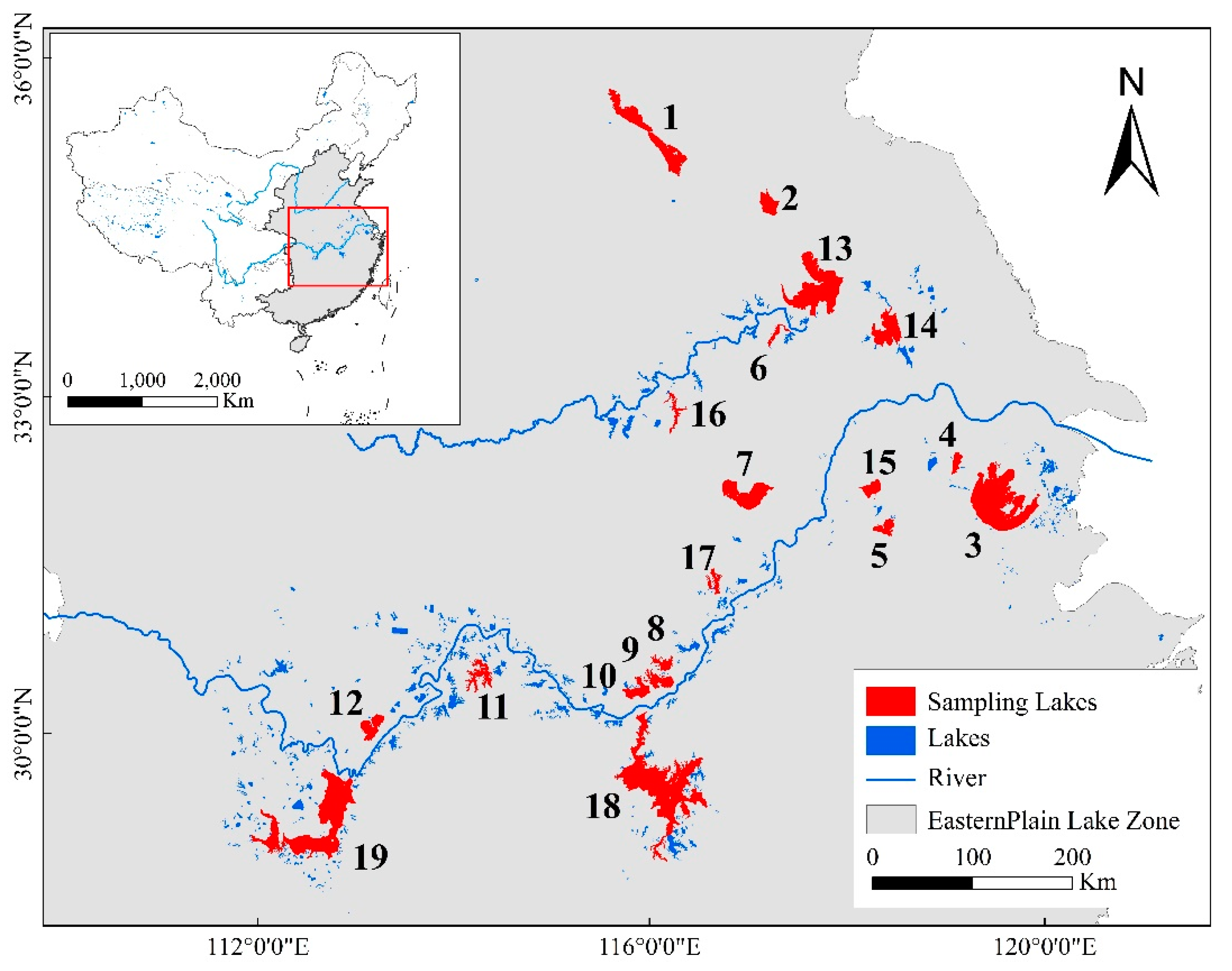
The Eastern Plain Lake (EPL) zone (18.1–42.6° N, 104.5–122.7° E) (Figure 1), as the core region of China, contains the most concentrated area of shallow water lakes in China with a dense population and developed economy [73,74]. The EPL zone contains 605 natural lakes larger than 1 km2 distributed in the middle and lower reaches of the Yangtze River (MLYR) basin, the Huai River (HR) basin, and the lower reaches of the Yellow River (LYR) basin [75,76,77,78,79,80]. The EPL zone belongs to the subtropical monsoon climate [81,82] and has the most representative and largest concentration of freshwater lakes in China [83]. These lakes are shallow with average depths from 1.1 to 8.4 m [21], providing sufficient water resources and promoting the development of the local economy [84]. Due to the influence of human activities, the water quality of the EPL zone is deteriorating and facing serious eutrophication with frequent occurrence of algal blooms [2,85,86].
2.2. Data Acquisition
2.2.1. Field Measurement
A total of 595 samples were taken from 19 lakes in the EPL zone during the 2013–2019 period (Figure 1, Table 1). The field experiments were carried out in clear weather and low wind speed (below 3 m/s).
Remote sensing reflectance (sr−1) at the wavelength (λ) (Rrs(λ)) of each field site, ranging from 350 nm to 1050 nm with an interval of 1 nm, was measured using an ASD field spectrometer (FieldSpec Pro Dual VNIR, Analytical Spectra Devices, Inc., Ann Arbor, MI, USA) with viewing direction of 45 deg. from the nadir and 135 deg. to the sun [87,88,89]. The value of the Fresnel reflectance ρ was assumed to be 0.028 according to the wind speed and sky conditions from field data and was then used to derive Rrs from the measured total water-leaving radiance (Lsw), the radiance of the gray panel (Lp), and sky radiance (Lsky) [21,88]. Furthermore, Landsat-8 spectral response functions (SRF) were used to simulated OLI Rrs(λ) based on the measured Rrs(λ) at each site, which was calculated to evaluate the accuracy with the bands of Landsat-8 data.
The Secchi disk depth (SDD, m), which reflects water transparency, was recorded using a standard 20 cm diameter Secchi disk when it cannot be observed in the water anymore [59,90,91]. Water samples were collected near the water surface (depth: ~0.50 m) using a 2-L polyethylene water-sampler and stored in the dark at 4 ℃ before laboratory analysis [21]. Water samples were filtered through a 47-mm Whatman GF/F glass fiber filter and Chlorophyll-a (Chla, μg/L) was extracted using 90–99.5% acetone, and then its concentration was measured spectrophotometrically [92,93,94]. The suspended particulate matter (SPM, mg/L) and the suspended particulate inorganic matter (SPIM, mg/L) were determined gravimetrically according to the Chinese national standard (GB11901-89,1990) [95]. Samples were filtered through Whatman GF/F filters, which had been combusted at 550 °C for 4 h and pre-weighted. SPM was dried at 105 °C for 4 h and weighed. SPIM was obtained through re-combusted at 550 °C for 4 h. Suspended particulate organic matter (SPOM, mg/L) was acquired by subtracting SPIM from SPM [95]. The concentration of total phosphorus (TP) and total nitrogen (TN) were analyzed by inductively coupled plasma atomic emission spectrometry (ICP-AES) [96,97].
We also investigated the lakes in the Yunnan-Guizhou plateau lake (TGPL) zone and obtained the measured Rrs(λ), SDD, Chla, and SPM of Lake Dianchi (N = 12) and Lake Erhai (N = 76), which were used to examine the applicability of the algorithm.
2.2.2. Satellite Images Processing
Landsat-8 OLI Surface Reflectance (SR) Tier 1 data, which provides 11 bands with a spatial resolution of 30 m, were generated from the Landsat Surface Reflectance Code (LaSRC) algorithm [1] and used in this study. Pixel quality attributes were generated from the C Function of Mask (CFMask) algorithm, including a cloud, shadow, water, and snow mask as well as a per-pixel saturation mask [98]. With a higher signal-to-noise ratio (SNR) and an additional band of 443 nm, the capability of Landsat-8 OLI was improved for retrieving water quality parameters and monitoring complex inland waters [99,100]. In this study, π is placed in the denominator to scale the surface reflectance to the water-leaving reflectance, and its formula see (1) [101]:
where Rrs (λ) is the water-leaving reflectance of OLI band centered at λ, SR(λ) is the original surface reflectance of OLI band centered at λ. The purpose of this conversion is to evaluate the accuracy of product band data.
Landsat-8 OLI SR product data were processed and analyzed through a cloud platform named Google Earth Engine (GEE, http://earthengine.google.com, accessed 16 April 2021), which provides massive global geospatial data and algorithms with minimal cost and equipment [98,102,103]. A total of 1505 OLI cloud-free images from 2013 to 2020 in the EPL zone were acquired in this study. The spatial distribution of OLI good observation images was shown in Figure S1, and the number of images counted by Landsat-8 path number and row number was shown in Figure S2.
Modification of normalized difference water index (MNDWI) was used to identify water bodies, which can be expressed as (2) [104]:
where Green and MIR are the green and the middle infrared band, separately. In this study, MIR refers to the Landsat-8 SWIR1 band. The modified histogram bimodal method was then used to define the threshold of each lake and extract water bodies automatically [105].
2.3. TSI Estimation from OLI Imagery
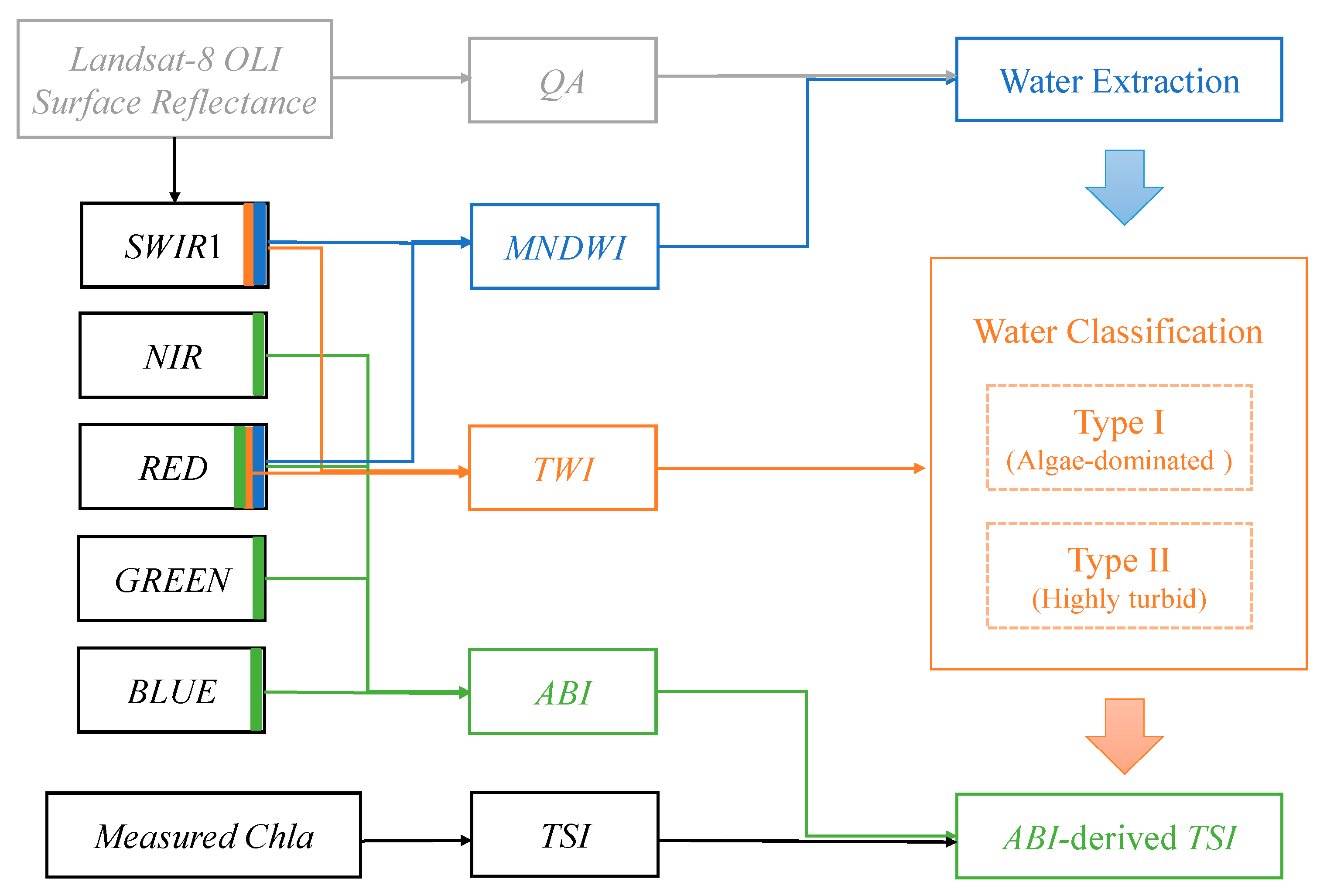
We developed the model for TSI retrieval for two optical water types because optical signals can be influenced under a high concentration of suspended sediments, leading to the misidentification of high turbidity as cyanobacterial scums [106]. Turbid water index (TWI) [106] was employed to classify algae-dominated and turbid water for each pixel from Landsat 8 images. Carlson’s trophic state index (TSI) was used to quantify the trophic status in studied lakes here, as it is commonly adopted for guiding and managing ecosystems and the water quality of inland waters [11,12,107]. The algal biomass index (ABI) [66] was used to derive TSI value with synchronous Landsat 8 surface reflectance images. The simulated values were compared with the in situ measured TSI to evaluate the accuracy of the algorithm. 493 random-selected samples supported the establishment of the algorithm, containing every sampling time. The rest of the samples (N = 102) were used for independent verification. The flow chart of the retrieval model was shown in Figure 2.
2.3.1. Turbid Water Index
The reflectance spectra of turbid waters and high chlorophyll-a waters showed significant differences in the red range and short-wave infrared range, which can be used to identify areas of high turbidity [84,106]. Therefore, the turbid water index (TWI) was used to extract turbid water and can be calculated from (3) [106].
In this study, the TWI value of each water sample was extracted from OLI SR data. Histogram statistics of TWI values with a mean (μ) and standard deviation (σ) were further calculated. The threshold of TWI for turbid water was 0.076 determined by μ − 2σ according to a 95% confidence interval. Therefore, water types were divided pixel by pixel based on OLI SR images of the studied lakes, where algae dominated-water was recorded as Type I and the extremely turbid water was recorded as Type II (see flow chart in Figure 2).
2.3.2. Trophic State Index
The trophic state index (TSI) is commonly adopted for guiding and managing the ecosystems and water quality of inland waters [11], which assumes algae biomass as the key descriptor for trophic state classification [12,16]. In this study, TSI was calculated based on Chla concentration and its formula see (4) [12].
2.3.3. Algal Biomass Index
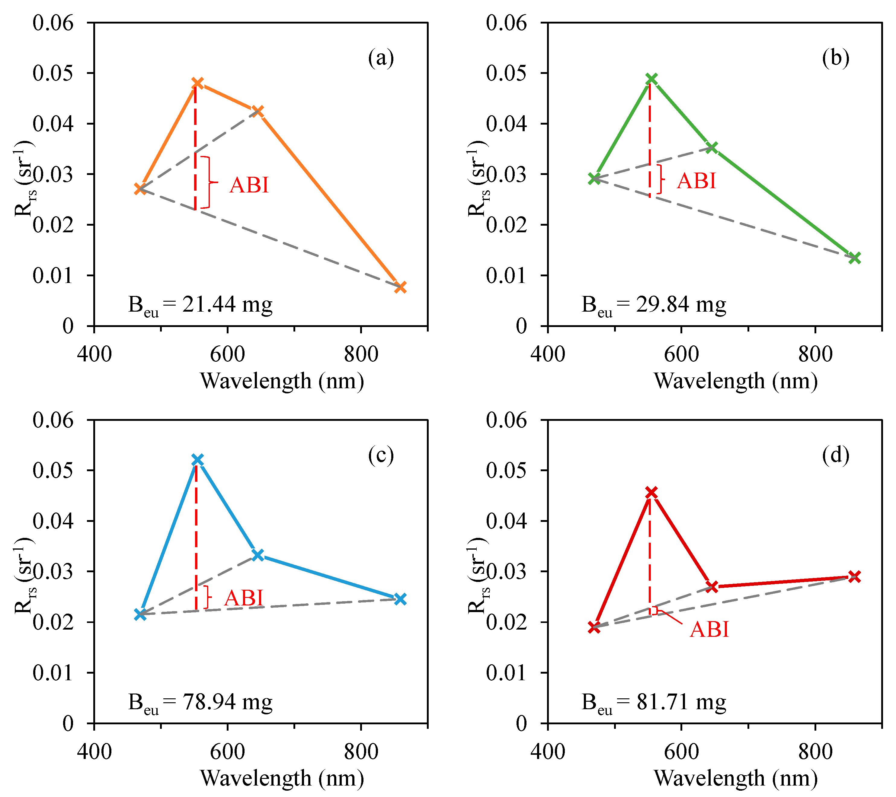
The algal biomass index (ABI) was originally proposed based on a Moderate-resolution imaging spectroradiometer (MODIS) to quantify the algal biomass in shallow lakes, which was proved a close relation with phytoplankton biomass in the water column [66]. The ABI uses the difference in remote-sensing reflectance (Rrs, sr−1) at 555 nm normalized against two baselines with one formed linearly between Rrs(859) and Rrs(469) and another formed linearly between Rrs(645) and Rrs(469) [66]. The structure of ABI was shown in Figure 3.
In this study, ABI was constructed based on OLI surface reflectance and defined as (5):
where BLUE, GREEN, RED, NIR, and SWIR are OLI SR data of 482, 561, 655, 865, and 1609 nm, λ is the wavelength at the corresponding band.
Comparisons between the ABI algorithm and other existing methods were further conduct to analyze the performance of the TSI model. We evaluated the performance of band ratio (BLUE/RED, NIR/RED) method [46,47,51], normalized difference vegetation index (NDVI) [54], enhanced vegetation index (EVI) [55], floating algae index (FAI) [18] and linear regression with multiple bands [57,58]. In addition, Cao et al. (2020) proposed a machine learning approach termed the extreme gradient boosting tree (BST) was employed to develop an algorithm for Chla estimation from Landsat 8 OLI in turbid lakes [21]. Therefore, the BST method utilizing all the spectral bands was examined to compare the results with ABI.
2.4. Accuracy Assessment
Five statistics were used for the ABI-derived TSI model’s assessment including the coefficient of determination (R2), root-mean-square error (RMSE), mean relative error (MRE), mean absolute error (MAE), and the Nash–Sutcliffe efficiency (NSE) [108,109,110,111].
These parameters are calculated as follows:
where Xi is the measured data, Yi is the simulated data of the ith sample, N is the number of samples. The NSE ranges from −∞ to 1, where 1 would mean the perfect observation-simulation match (which is not possible) and NSE = 0 indicates that the simulated data is commensurable with the variance of the measured data. When the value of NSE is close to 1, indicating good model quality and high model credibility [111,112].
3. Results
3.1. Characteristics of Water Quality Parameters in Sampling Lakes
The water quality parameters of the 595 water samples are listed in Table 2. The average Chla concentration was 34.72 ± 49.61 μg/L. In addition, the R2 between SPIM and SPM was 0.88 (p < 0.01, N = 595). In 80.8% of the water samples (N = 481), SPIM concentration accounted for more than 50% of SPM concentration, indicating that SPIM is the primary particle of SPM. The 89.7% of the investigated lakes (N = 534) had an average SDD below 0.5 m, and no lakes had an average SDD above 1.0 m. The average TSI of sampling lakes was 65.37 ± 11.49, illustrating the typical characteristics of shallow turbid eutrophic lakes.
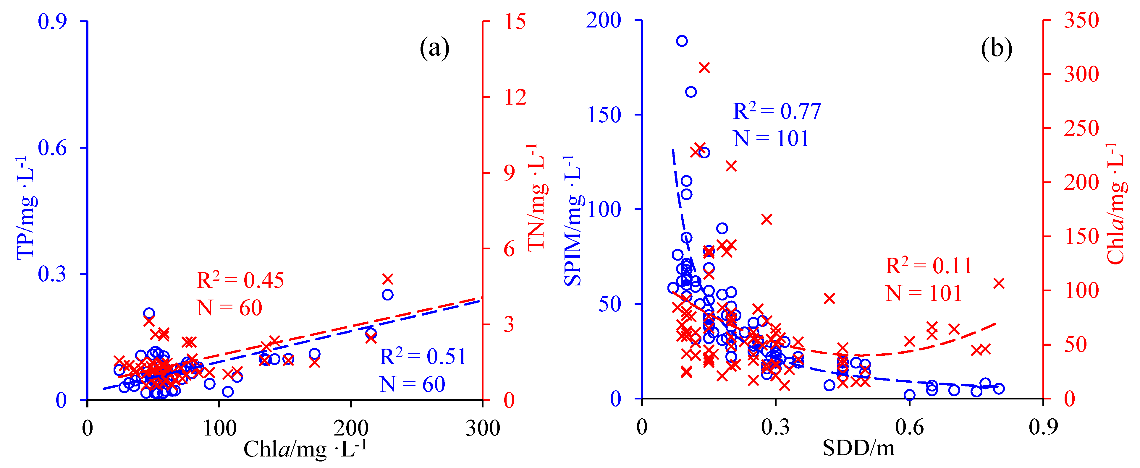
Significant correlations between Chla, and TN (R2 = 0.45, p < 0.01, N = 60) and TP (R2 = 0.51, p < 0.01, N = 60 because TN and TP were not measured every time) are shown in Figure 4a. The relationship between SDD, Chla, and SPIM is shown in Figure 4b. SDD showed a clear correlation with SPIM (R2 = 0.76, p < 0.01, N = 101) but showed no correlation with Chla (R2 = 0.07, N=101). Thus, the transparency of sampling lakes is greatly affected by SPIM.
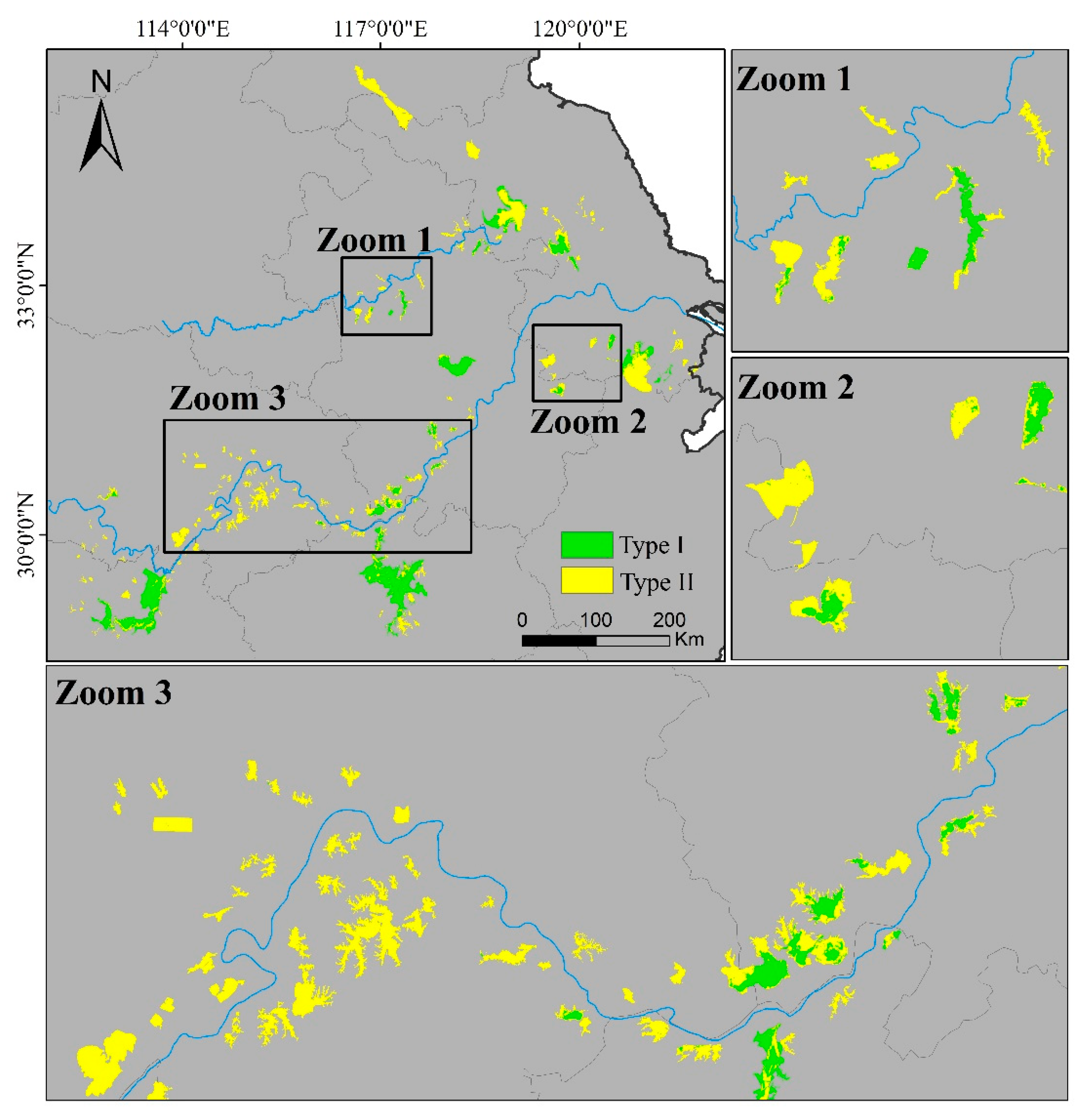
The map of water classification based on the TWI threshold for EPL lakes was shown in Figure 5. These lakes differ greatly in the proportion of turbid water and algal-dominated water. Turbid water bodies accounted for 86.30% of the total number and 50.11% of the total surface area. Our results have similar spatial distribution for extremely turbid water in the middle and lower reaches of the Yangtze and Huai Rivers [24,113]. Small lakes near the Yangtze River and the lake estuary were mainly turbid water due to the influence of the Yangtze River. For example, turbid water distributions of Lake Hongze followed a distinct pattern that surrounds the Huai River Estuary and expands toward the center of the lake. The highly turbid water of Lake Poyang appears in the north lake because of the sand dredging in the Yangtze River. These results are consistent with the previous studies [84,95].
3.2. Consistency of OLI Product Data
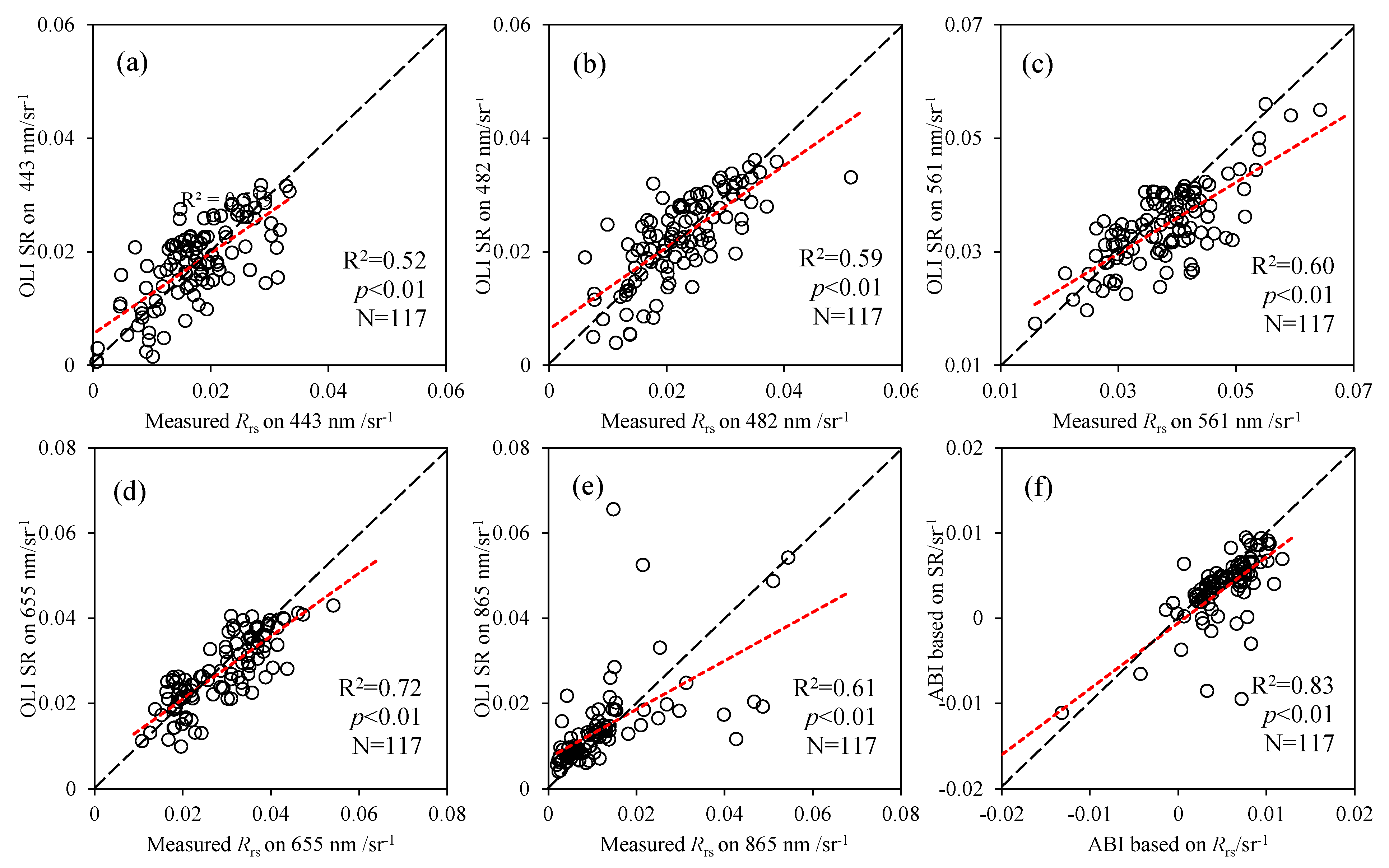
Relationships between in situ band-averaged and OLI-derived Rrs in each band and corresponding ABI are shown in Figure 6. The R2 correlation between OLI Rrs and synchronous simulated Rrs of each band was greater than 0.50 (p < 0.01, N = 117), and the red band had the highest correlation (R2 = 0.72, p < 0.01), followed by the green band (R2 = 0.60, p < 0.01), and the blue bands had the lowest R2 with a 0.57 for 482 nm and a 0.52 for 443 nm, respectively.
Table 3 analyzed the MAE, MRE, RMSE, and NSE of each band and ABI. The MRE of 443 and 482 nm in the blue bands was 34.43% and 24.01%, and the RMSE was 0.0055 and 0.0053 sr−1, respectively. The MRE of the green band was 13.96% and the RMSE was 0.0060 sr−1. The MRE and RMSE of the red band were the lowest at 14.60% and 0.0047 sr−1, respectively, while that of the NIR band, MRE and RMSE were the highest at 38.45% and 0.0097 sr−1, respectively. Performances of the green band (NSE = 0.92) and red band (NSE = 0.89) were better than that of the blue bands. Note that the correlation of OLCI Rrs and simulated Rrs in the NIR band was significant (R2 = 0.61, p < 0.01), but error statistics showed a low precision (RMSE = 0.0097, NSE = 0.38) due to the relatively lower value of the NIR band itself.
The correlation between ABI based on the simulated Rrs and OLI Rrs was further explored and R2 was as high as 0.83 (p < 0.01, N = 117, Figure 6f), which was better than that of the single band. The error statistics of the ABI algorithm (Table 3) showed that the MRE was 13.76%, and the RMSE was 0.0022 sr−1, which was more accurate than the single band and further reduced the uncertainty. The NSE of ABI based on the simulated Rrs and OLI Rrs was 0.97, illustrating a good model quality and credibility.
3.3. Performance of ABI-Derived TSI
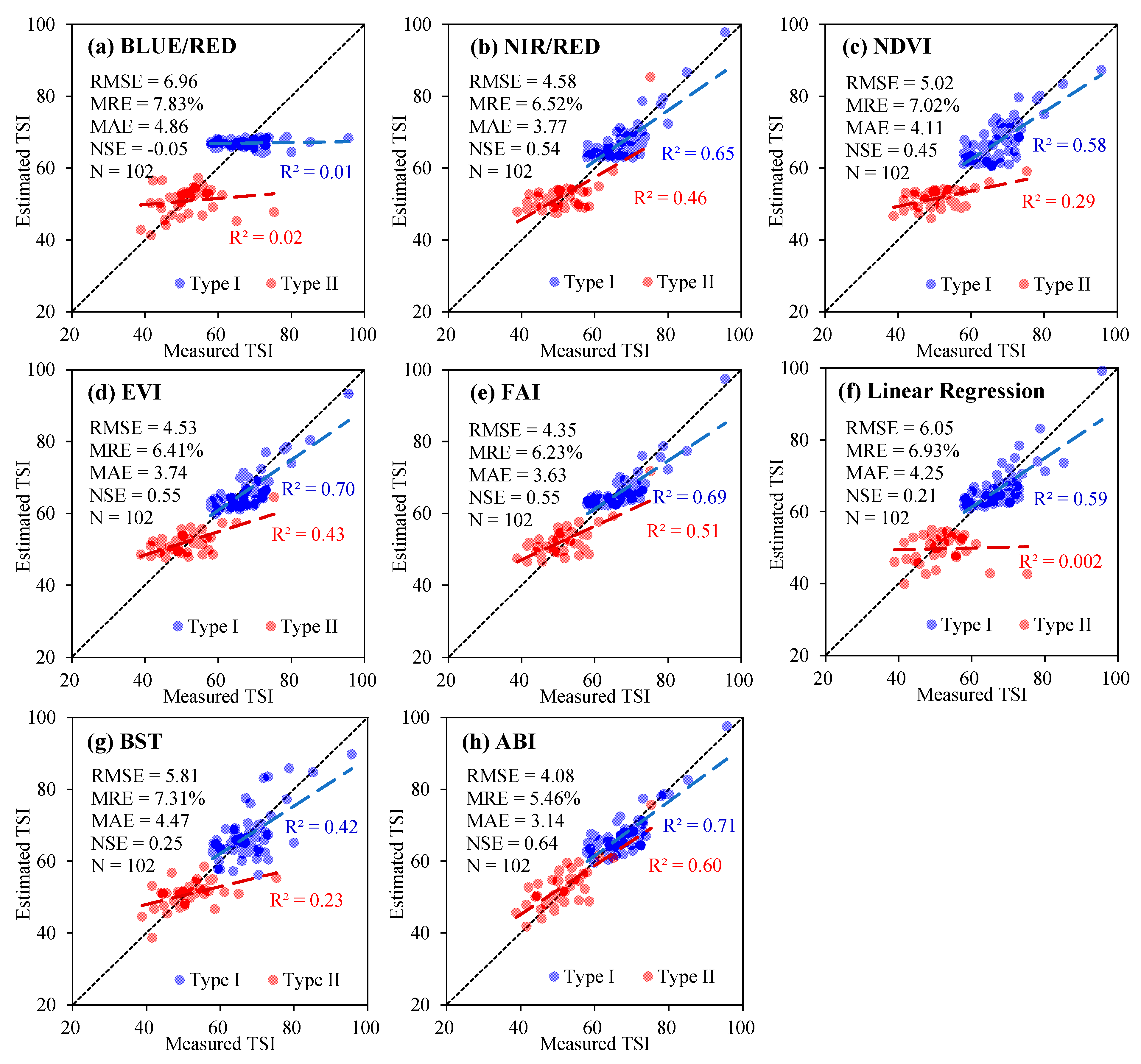
The relationship between ABI and TSI performed well on algae-dominated waters (Type I, N = 282, R2 = 0.62, p < 0.01) and turbid waters (Type II, N = 132, R2 = 0.57, p < 0.01, Figure S3h). The inversion accuracy of the ABI algorithm was shown in Figure 7h. The estimated TSI are uniformly distributed on the two sides of the 1:1 line (RMSE = 4.08, MRE = 5.46%, MAE = 3.14, and NSE = 0.64), indicating that the algorithm exhibits a relatively satisfactory degree of estimation accuracy for the high and low ranges and that it reaches a relatively satisfactory level of consistency. The precision of different fitting models for the ABI algorithm was listed in Table S1 and a linear model was finally chosen for the ABI-derived TSI. The fitting formula was confirmed as Equation (11) for Type I water and Equation (12) for Type II water:
The model based on ABI outperformed other state-of-the-art models on TSI retrievals. Most of the algorithms have achieved good precisions for training, but the accuracy for independent validation was not ideal. The BLUE/RED ratio showed no correlation with TSI both in training dataset (R2 = 0.02 for Type I and 0.42 for Type II, Figure S3a) and validation dataset (R2 = 0.01 for Type I and 0.02 for Type II, Figure 7a), showing the lowest precision (RMSE = 6.96, MRE = 7.83% and NSE = −0.05, Figure 7a).
NIR/RED for training showed an acceptable correlation for Type I (R2 = 0.52, p < 0.01) but no significant correlation for Type II (R2 = 0.12, Figure S3b). The accuracy of the NIR/RED ratio (RMSE = 4.58 and MRE = 6.52%, Figure 7b) was better than BLUE/RED ratio method.
Algorithms of NDVI, EVI and FAI showed the similar accuracy for training dataset with R2 > 0.49 for Type I and R2 < 0.21 for Type II (Figure S3c–e). The accuracy of FAI (RMSE = 4.35, MRE = 6.23%, MAE = 3.63 and NSE = 0.55, Figure 7e) performed better than that of NDVI (RMSE = 5.02, MRE = 7.02%, MAE = 4.11 and NSE = 0.45, Figure 7c) and EVI (RMSE = 4.53, MRE = 6.41%, MAE = 3.74 and NSE = 0.55, Figure 7d).
The linear regression for training dataset showed a relatively higher correlation (R2 = 0.55 for Type I and 0.42 for Type II, Figure S3f) than three indexes, and the correlation for validation performed well in Type I (R2 = 0.59) but showed underestimation in Type II (R2 = 0.002), which affected the accuracy of validation (RMSE = 6.05, MRE = 6.93% and NSE = 0.21, Figure 7f).
BST algorithm has the highest correlation for training (R2 = 0.89 for Type I and 0.79 for Type II, Figure S3g) but the lowest correlation for validation (R2 = 0.42 for Type I and 0.23 for Type II, Figure 7g). The accuracy of the BST algorithm for the validation dataset (RMSE = 5.81, MRE = 7.31% and NSE = 0.25, Figure 7g) was also not as good as the training dataset, and even worse than the band ratio method.
The accuracy of the ABI-based trophic state classification showed that 82.35% (N = 84) of the retrieval TSI were consistent with the measured results. 31.25% of the mesotrophic water bodies were overestimated as eutrophic, 6.15% of the eutrophic water bodies were underestimated as mesotrophic, 3.07% of the eutrophic water bodies were overestimated as hypertrophic, and 33.33% of the hypertrophic water bodies were underestimated as eutrophic.
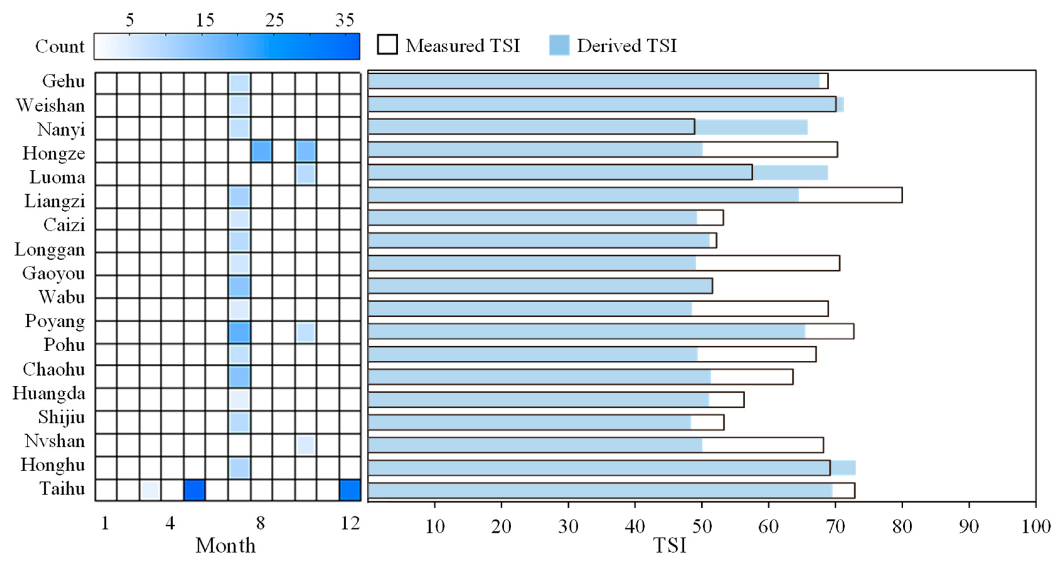
The average TSI of 19 sampling lakes in 2018 was shown in Figure 8 to quantify the trophic state level. The comparison with the measured TSI in the same year showed that nine lakes of ABI-derived TSI were consistent with the measured results. However, the other 10 lakes of the estimated TSI were lower than the measured TSI. This is because the sampling time is concentrated in summer (from July to October, Figure 8) when high algal reproduction and growth occurs, and eutrophication is more severe than in other seasons.
3.4. Spatial Distribution of TSI for Lakes in the EPL
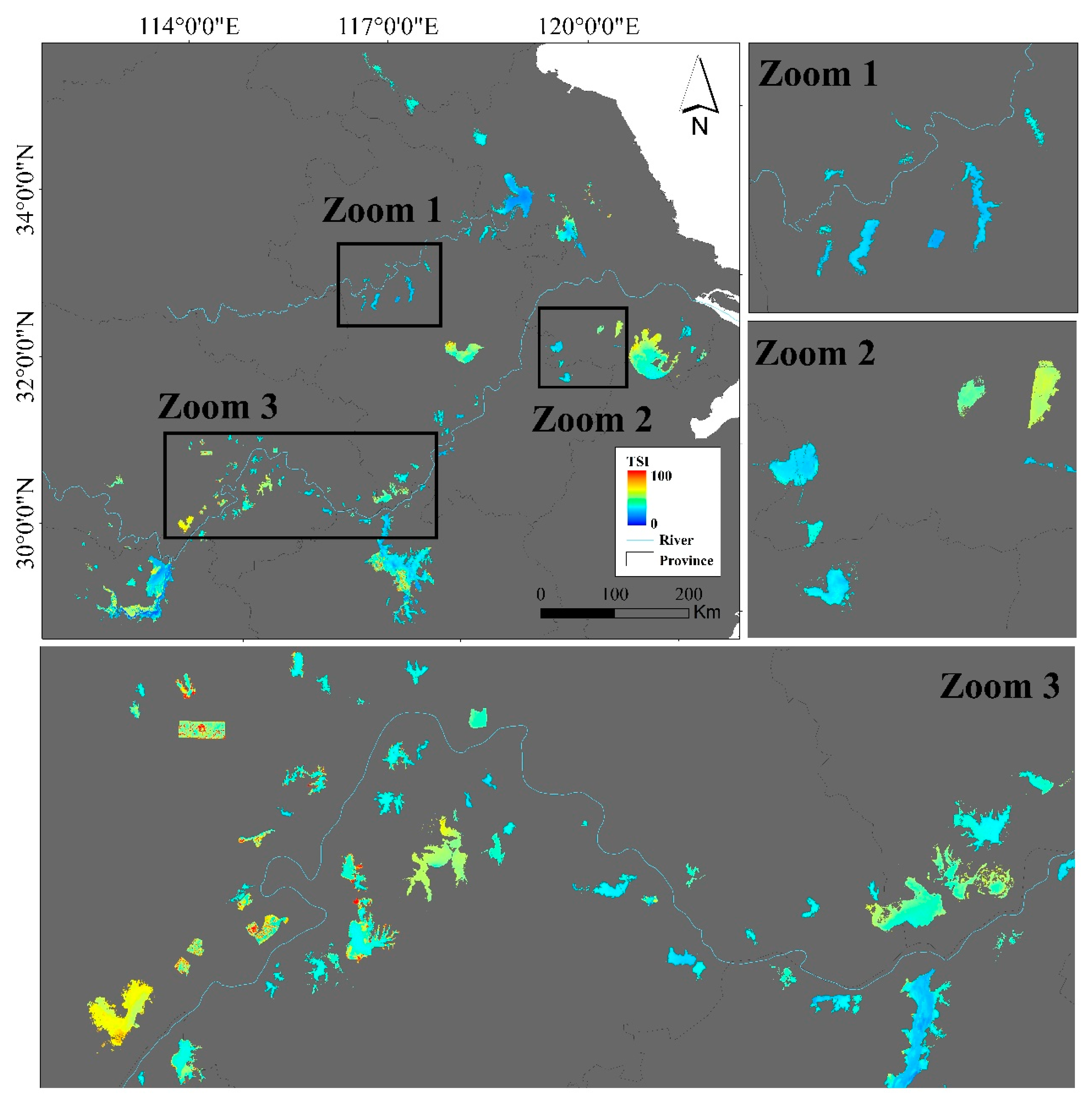
The TSI of lakes larger than 10 km2 in the EPL zone (N = 146, total surface area = 19,752.84 km2) in 2018 was shown in Figure 9. From the spatial distribution perspective, the TSI of Lake Taihu, Chaohu, and small lakes near the Yangtze River were noticeably high and eutrophic. Lake Poyang, Dongting, and lakes near the Huai River had a relatively lower TSI and were mesotrophic. The north of Lake Chaohu and Taihu had a higher TSI, and the nearshore trophic state was higher than that of the central area.
The ABI-derived TSI of lakes in 2018 ranged from 24.28 to 74.35. Hypertrophic lakes accounted for 14.38% of the total number but only 5.17% of the total surface area, eutrophic lakes accounted for 55.48% of the total number and 34.23% of the total surface area, mesotrophic lakes accounted for 28.77% of the total number but 58.90% of the total surface area, and oligotrophic lakes accounted for 1.37% of the total number and 1.69% of the total surface area.
3.5. Temporal Dynamics of TSI for Lakes in the EPL
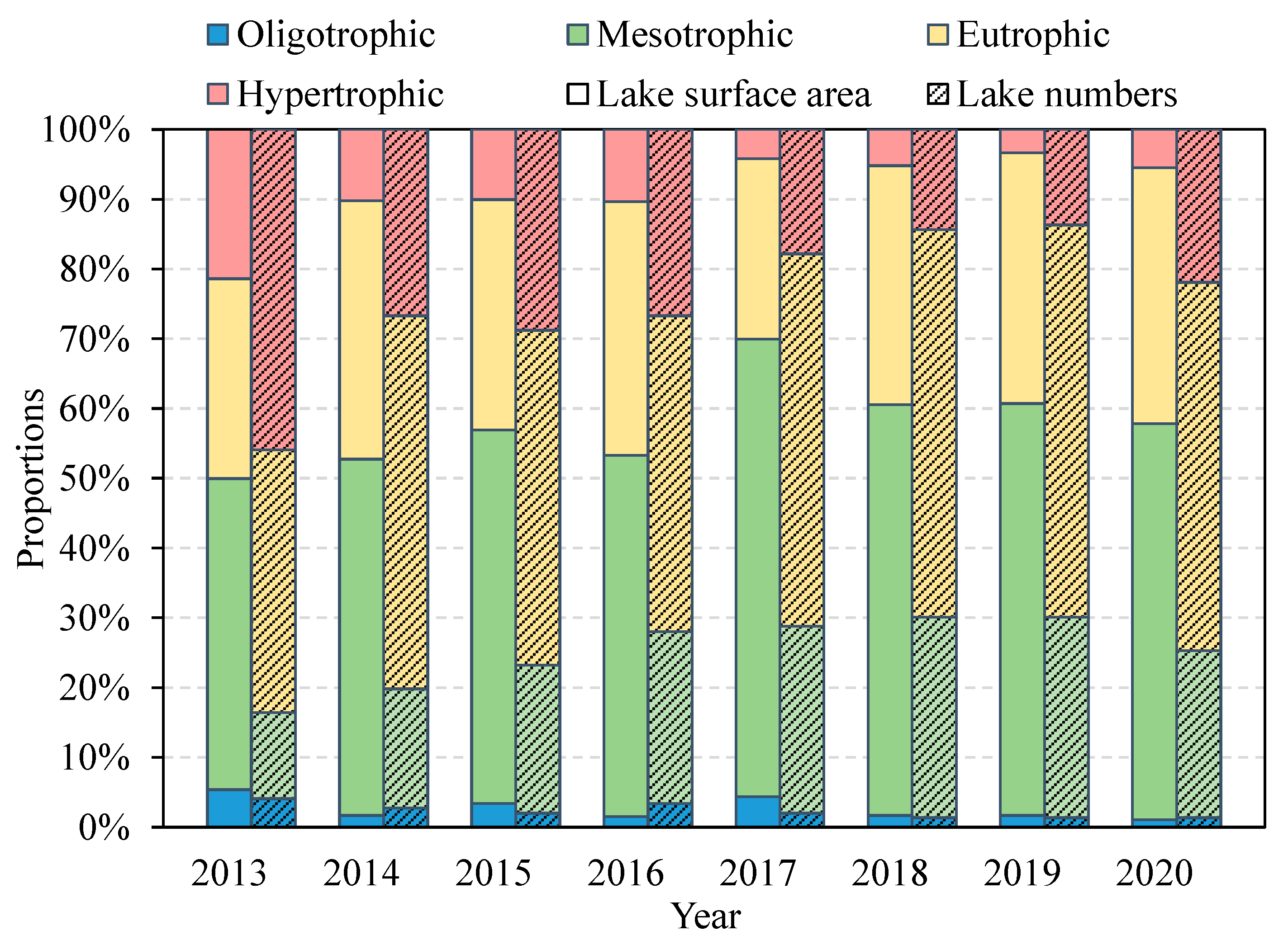
The trophic state of 146 lakes in the EPL from 2013 to 2020 was further assessed. Figure 10 illustrates the proportion of each lake with a trophic state according to the lake number and lake surface area. In terms of lake number, the number of hypertrophic and oligotrophic lakes decreased from 45.89% to 21.92% and 4.11% to 1.37%, respectively, while the number of mesotrophic and eutrophic lakes increased from 12.33% to 23.97% and 37.67% to 52.74%. In terms of water surface area, the hypertrophic water area decreased in the past eight years (from 21.39% to 5.49%), while that of mesotrophic water noticeably increased from 44.56% to 56.75%, indicating that the trophic state of lakes decreased.
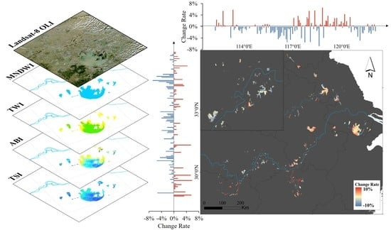
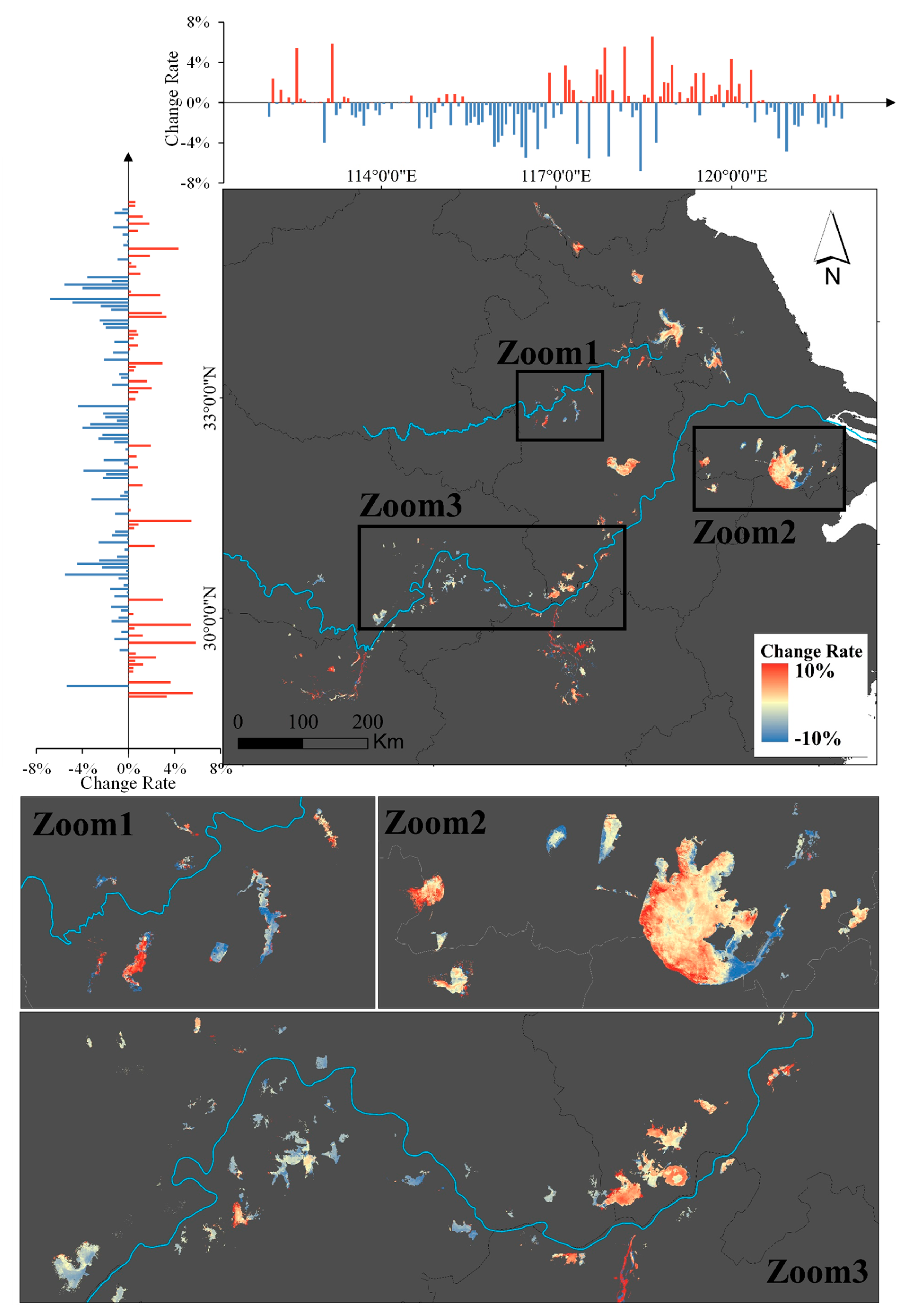
The relative change rate of TSI of each lake in eight years was shown in Figure 11. According to the geometric center of lakes, the bar chart on the top and left were the statistics of the relative change rate sorted by longitude and latitude. From the longitude perspective, the TSI change rate of small lakes in the MLYR basin in 2020 was negative compared with that in 2013, indicating that the trophic state has decreased, and the water quality has improved. However, the eutrophication of small lakes along the lower reaches of the Yangtze River is still severe. In terms of latitude, there is no apparent bias in the change rate. The change rate of the negative TSI in the HR basin is higher than that in the MLYR basin, and the change rate of the positive TSI in the MLYR basin is higher than that in the HR basin, indicating that the water quality of lakes in the HR basin improved faster than that in the MLYR basin. In contrast, the water quality of the lakes in the Yangtze River basin deteriorates faster owing to the demand for domestic and industrial water for human activities. Therefore, lake eutrophication monitoring and management is still an urgent and long-term project.
4. Discussion
4.1. Limits of Algorithm
It is the perfect solution to assess the trophy based on Carlson’s trophic state index, including SDD, chlorophyll, and TP. However, it is a challenge to estimate them through optical remote sensing [114]. Overall, TSI(Chla) was an appropriate index than TSI(SDD) and TSI(TP) to evaluate the trophic state in the eastern Chinese lakes. Zou et al. (2020) discussed limitations of TSI based on SDD, which can be easily affected by non-algal turbidity and cannot provide an accurate indication of algal biomass [115,116]. The comparison of measured SDD with measured SPIM and Chla (Figure 4b) in our study showed 0.77 of R2 between SDD and SPIM concentration, while 0.11 of R2 between SDD and Chla concentration, illustrating the influence of SDD under high SPIM and could misjudge the trophic state. Comparison of TSI(Chla) and TSI(Chla, SDD, and TP) showed an acceptable precision that 79.55% of samples were at the same trophic level (Figure S4). Therefore, TSI(Chla) performed well for lakes in the EPL zone, which may represent the TSI results based on multi parameters.
In this study, trophic states of 19 sampling lakes were above the level of mesotrophic, which lacked the validation for oligotrophic water or clean water. One of the baselines was built using the blue and NIR bands, which made it possible to detect increasing algal biomass through the uplift reflectance of the NIR band. The entire spectral reflectance was low for clean water and showed no evident fluctuations in the NIR band [117], which may not be applicable for clean water to obtain good inversion results. Therefore, the classification of lakes will be developed for future studies to improve inversion accuracy.
The accuracy of ABI-derived TSI in turbid water was not as satisfactory (R2 = 0.57 for training and 0.60 for validation) as that in algae-dominated water (R2 = 0.62 for training and 0.71 for validation). A previous study has verified that the ABI algorithm is more sensitive to the change of SPIM [66]. When the change rate of SPIM is 10%, 50%, and 100%, the corresponding relative errors of ABI are 6.94%, 28.19%, and 54.75%, respectively [66]. Although we used TWI to extract turbid water and established the TSI algorithm for turbid water, the overestimation of TSI caused by extremely turbid water cannot be ignored.
In addition, a revisit period of 16 days for Landsat-8 OLI limits the frequency of lake observations, especially for lakes in the eastern plain of China. The subtropical monsoon climate in the eastern plain leads to more precipitation, more clouds, and relatively fewer images in summer, which will also have an impact on the annual average statistical results of TSI. We will use the application of the algorithm in other satellites (such as MODIS or OLCI) to improve the observation frequency and make the evaluation results of the trophic state more accurate.
4.2. Prospects of Algorithm
4.2.1. Applicability to Other Sensors
The application of the ABI algorithm to moderate-resolution imaging spectroradiometer (MODIS) and Sentinel-3 OLCI sensors was explored, as the 16-day temporal resolution of Landsat-8 OLI cannot provide a continuous observation. In terms of Type I, the R2 of MODIS-based and Sentinel-3 OLCI-based ABI with TSI were 0.51 (p < 0.01, N = 286) and 0.50 (p < 0.01, N = 244), respectively, indicating a good correlation. The correlation for Type II lakes was 0.44 (p < 0.01, N = 241) and 0.46 (p < 0.01, N = 165), respectively.
Classification of trophic state level based on two sensors showed the overall accuracy of 83.27% for MODIS and 82.92% for OLCI. For MODIS, 67.82% of the mesotrophic water bodies, 88.67% of the eutrophic water bodies, and 79.79% of the hypertrophic water bodies were accurately classified. For OLCI, 82.22 % of the mesotrophic water bodies, 87.59% of the eutrophic water bodies, and 72.41% of the hypertrophic water bodies were accurately classified. Although the correlation of the two sensors were both lower than that of Landsat-8 OLI because of the low spatial resolution (250 and 500 m for MODIS, and 300 m for OLCI), the overall accuracy of the trophic state classification based on these two sensors were both more than 80%. This may be due to the clustering process for trophic state classification, which further reduced the error. Therefore, MODIS and OLCI can still be used to supply high-frequency observations. The scatter plot between ABI based on synchronous MODIS and OLCI was shown in Figure S5 and the precision of ABI-derived TSI based on MODIS and OLCI sensors were listed in Table S2.
4.2.2. Applicability to Other Lakes
The Pearson correlation analysis of the ABI algorithm showed the significant correlation for Lake Dianchi (r = 0.86, p < 0.01, N = 12) and Lake Erhai (r = 0.68, p < 0.01, N = 76), which are two representative lakes in the Yunnan-Guizhou plateau lake (TGPL) zone [118]. Statistics of Chla, SDD, and Pearson correlation analysis between ABI(SR) and measured TSI of Lake Dianchi and Lake Erhai were listed in Table S3. The fitting accuracy of the ABI algorithm for two lakes was acceptable with an R2 = 0.83 (p < 0.01, N = 60, Figure S6a). Independent verification showed an RMSE of 4.22 and an MRE of 0.06 (N = 28, Figure S6b).
The spatial distribution of ABI-derived TSI with Landsat-8 OLI RGB images (stretched by histogram specification) of Lake Erhai on June 6 and Lake Dianchi on August 11, 2019, is shown in Figure S7. Lake Erhai was mainly mesotrophic, and the northern lake and lakeshore were eutrophic. In contrast, Lake Dianchi was eutrophic, and floating algae appeared in the center and north of the lake, which made the water body in this area severely hypertrophic. The spatial distribution of eutrophication is consistent with that of algae, indicating the applicability and potential of the ABI algorithm.
5. Conclusions
In this study, a retrieval algorithm for trophic state assessment of inland waters was developed based on Landsat 8 OLI surface reflectance imagery. This algorithm provides the ability to retrieve TSI in turbid lakes and identifies spatial distributions of the trophic state in lakes. The high consistency between the OLI Rrs and the measured Rrs proves the potential of OLI surface reflectance in eutrophication evaluation.
Assessments of trophic state with 146 lakes larger than 10 km2 in eastern China from 2013 to 2020 were implemented on OLI images. Eutrophic lakes decreased in the past eight years, while 3.00% of the oligotrophic lakes gradually became eutrophic. Hypertrophic and eutrophic lakes were mainly concentrated in the lower reaches of the Yangtze River basin, mesotrophic and oligotrophic water bodies were mainly concentrated in the middle reaches of the Yangtze River and Huai River basin. However, the misjudgment caused by extremely turbid water cannot be ignored and the applicability of the TSI retrieval model trained from EPL lakes was limited by the range of the dataset, demonstrating that the coefficient of the TSI model needs to be adjusted before applying to other regions.
Supplementary Materials
The following are available online at https://0-www-mdpi-com.brum.beds.ac.uk/article/10.3390/rs13101988/s1, Figure S1. Landsat-8 OLI coverage of observation and number of good observations from 2013 to 2019. Figure S2. Number of OLI images counted by Landsat-8 path and row. Figure S3. Correlations of different method based on surface reflectance (SR) and measured trophic state index (TSI): (a) BLUE/RED, (b) NIR/RED, (c) normalized difference vegetation index (NDVI), (d) enhanced vegetation index (EVI), (e) floating algae index (FAI), (f) linear regression, (g) the extreme gradient boosting tree (BST), and (h) algal biomass index (ABI). Figure S4. Comparison of the TSI(Chla) and (a) TSI(SDD), (b)TSI (SDD, Chla), (c) TSI(SDD, TP) and (d) TSI(TP, Chla, SDD). Figure S5. Application of ABI algorithm based on (a) MODIS; (b) OLCI. Figure S6. (a) Performance of ABI-derived TSI for lakes in the Yunnan-Guizhou plateau lake (TGPL) zone and (b) independent validation. Figure S7. Landsat-8 OLI RGB images (stretched by histogram specification) of (a) Lake Erhai on June 6 and (c) Lake Dianchi on 11 August 2019; and simulated TSI of (b) Lake Erhai and (d) Lake Dianchi. Table S1. Correlation and precision with a different fitting model. Table S2. Accuracy of trophic state classification based on ABI algorithm for MODIS and OLCI. Table S3. Statistics of Chla, SDD of Lake Dianchi and Lake Erhai, and Pearson correlation analysis between ABI(SR) and measured TSI.
Author Contributions
Conceptualization, M.H. and R.M.; methodology, M.H.; software, M.H. and Z.C.; validation, M.H., Z.C. and J.X.; formal analysis, M.H. and Z.C.; investigation, R.M.; resources, J.X. and K.X.; data curation, M.H. and J.X.; writing—original draft preparation, M.H.; writing—review and editing, Z.C. and J.X; visualization, M.H. and K.X.; supervision, R.M.; project administration, K.X. and R.M.; funding acquisition, R.M. All authors have read and agreed to the published version of the manuscript.
Funding
This research was funded by the National Natural Science Foundation of China (Grant No. 42071341).
Institutional Review Board Statement
Not applicable.
Informed Consent Statement
Not applicable.
Data Availability Statement
The data presented in this study are available upon request from the corresponding author.
Acknowledgments
The authors thank the study participants from NIGLAS (Dian Wang, Zhigang Cao, Junfeng Xiong, Ming Shen, Tianci Qi, Jinge Ma, Qiao Chu, and Pengfei Zhan). Dataset of EPL lakes was supported by National Geographic Resource Science SubCenter, National Earth System Science Data Center, National Science & Technology Infrastructure of China (http://gre.geodata.cn, accessed on 16 April 2021).
Conflicts of Interest
The authors declare that they have no conflict of interest.
References
- Deng, Y.; Jiang, W.; Tang, Z.; Ling, Z.; Wu, Z. Long-Term Changes of Open-Surface Water Bodies in the Yangtze River Basin Based on the Google Earth Engine Cloud Platform. Remote Sens. 2019, 11, 2213. [Google Scholar] [CrossRef] [Green Version]
- Song, K.; Liu, G.; Wang, Q.; Wen, Z.; Lyu, L.; Du, Y.; Sha, L.; Fang, C. Quantification of lake clarity in China using Landsat OLI imagery data. Remote Sens. Environ. 2020, 243, 111800. [Google Scholar] [CrossRef]
- Pekel, J.-F.; Cottam, A.; Gorelick, N.; Belward, A.S. High-resolution mapping of global surface water and its long-term changes. Nature 2016, 540, 418–422. [Google Scholar] [CrossRef]
- Smith, V.H. Eutrophication of freshwater and coastal marine ecosystems a global problem. Environ. Ence Pollut. Res. Int. 2003, 10, 126. [Google Scholar] [CrossRef]
- Ho, J.C.; Michalak, A.M.; Pahlevan, N. Widespread global increase in intense lake phytoplankton blooms since the 1980s. Nature 2019, 574, 667–670. [Google Scholar] [CrossRef]
- Le, C.; Zha, Y.; Li, Y.; Sun, D.; Lu, H.; Yin, B. Eutrophication of Lake Waters in China: Cost, Causes, and Control. Environ. Manag. 2010, 45, 662–668. [Google Scholar] [CrossRef]
- Hu, M.; Zhang, Y.; Ma, R.; Zhang, Y. Spatial and Temporal Dynamics of Floating Algae Blooms of Lake Chaohu in 2016 and Environmental drivers. Environ. Sci. 2018, 39, 4925–4937. [Google Scholar]
- Hatvani, I.G.; Barros, V.D.D.; Tanos, P.; Kovacs, J.; Clement, A. Spatiotemporal changes and drivers of trophic status over three decades in the largest shallow lake in Central Europe, Lake Balaton. Ecol. Eng. 2020, 151, 105861. [Google Scholar] [CrossRef]
- Adamovich, B.V.; Zhukova, T.V.; Mikheeva, T.M.; Kovalevskaya, R.Z.; Yanova, E. Long-term variations of the trophic state index in the Narochanskie Lakes and its relation with the major hydroecological parameters. Water Resour. 2016, 43, 809–817. [Google Scholar] [CrossRef]
- Dodds, W.K. Trophic state, eutrophication and nutrient criteria in streams. Trends Ecol. Evol. 2007, 22, 669–676. [Google Scholar] [CrossRef] [PubMed]
- Shi, K.; Zhang, Y.; Song, K.; Liu, M.; Qin, B. A semi-analytical approach for remote sensing of trophic state in inland waters: Bio-optical mechanism and application. Remote Sens. Environ. 2019, 232, 111349. [Google Scholar] [CrossRef]
- Carlson, R.E. A Trophic State Index for Lakes. Limnol. Oceanogr. 1977, 22, 361–369. [Google Scholar] [CrossRef] [Green Version]
- Aizaki, M.; Otsuki, A.; Fukushima, T.; Hosomi, M.; Muraoka, K. Application of Carlson’s trophic state index to Japanese lakes and relationships between the index and other parameters. Proc. Int. Assoc. Theor. Appl. Limnol. 1981, 16, 19–22. [Google Scholar] [CrossRef]
- Li, Z.; Zhang, H. Trophic state index and its correlation with lake parameters. Acta Sci. Circumstantiae 1993, 13, 391–397. [Google Scholar] [CrossRef]
- Vollenweider, R.A.; Kerekes, J. Eutrophication of waters. Monitoring, assessment and control. In OECD Cooperative Programme on Monitoring of Inland Waters (Eutrophication Control). Environment Directorate; OECD: Washington, DC, USA, 1982; p. 154. [Google Scholar]
- Carlson, R.E.; Havens, K.E. Simple Graphical Methods for the Interpretation of Relationships Between Trophic State Variables. Lake Reserv. Manag. 2005, 21, 107–118. [Google Scholar] [CrossRef]
- Walsh, J.R.; Carpenter, S.R.; Zanden, M.J.V. Invasive species triggers a massive loss of ecosystem services through a trophic cascade. Proc. Natl. Acad. Sci. USA 2016, 113, 201600366. [Google Scholar] [CrossRef] [PubMed] [Green Version]
- Hu, C.M. A novel ocean color index to detect floating algae in the global oceans. Remote Sens. Environ. 2009, 113, 2118–2129. [Google Scholar] [CrossRef]
- Thiemann, S.; Kaufmann, H. Determination of Chlorophyll Content and Trophic State of Lakes Using Field Spectrometer and IRS-1C Satellite Data in the Mecklenburg Lake District, Germany. Remote Sens. Environ. 2000, 73, 227–235. [Google Scholar] [CrossRef]
- Wang, Z.; Hong, J.; Du, G. Use of satellite imagery to assess the trophic state of Miyun Reservoir, Beijing, China. Environ. Pollut. 2008, 155, 13–19. [Google Scholar]
- Cao, Z.; Ma, R.; Duan, H.; Pahlevan, N.; Melack, J.; Shen, M.; Xue, K. A machine learning approach to estimate chlorophyll-a from Landsat-8 measurements in inland lakes. Remote Sens. Environ. 2020, 248, 111974. [Google Scholar] [CrossRef]
- Le, C.; Li, Y.; Zha, Y.; Sun, D. Euphotic depth: Retrieval from in situ reflectance and application in assessing eutrophication. Acta Ecol. Sin. 2008, 28, 2614–2621. [Google Scholar]
- Butt, M.J.; Nazeer, M. Landsat ETM+ Secchi Disc Transparency (SDT) retrievals for Rawal Lake, Pakistan. Adv. Space Res. 2015, 56, S0273117715004780. [Google Scholar] [CrossRef]
- Liu, D.; Duan, H.; Yu, S.; Shen, M.; Xue, K. Human-induced eutrophication dominates the bio-optical compositions of suspended particles in shallow lakes: Implications for remote sensing. Sci. Total Environ. 2019, 667, 112–123. [Google Scholar] [CrossRef] [PubMed]
- Iwashita, K.; Kudoh, K.; Fujii, H.; Nishikawa, H. Satellite analysis for water flow of Lake Inbanuma. Adv. Space Res. 2004, 33, 284–289. [Google Scholar] [CrossRef]
- Chen, Q.; Huang, M.; Tang, X. Eutrophication assessment of seasonal urban lakes in China Yangtze River Basin using Landsat 8-derived Forel-Ule index: A six-year (2013–2018) observation. Sci. Total Environ. 2020, 745, 135392. [Google Scholar] [CrossRef]
- Wang, S.; Li, J.; Bing, Z.; Spyrakos, E.; Tyler, A.; Shen, Q.; Zhang, F.; Kuster, T.; Lehmann, M.; Wu, Y.; et al. Trophic state assessment of global inland waters using a MODIS-derived Forel-Ule index. Remote Sens. Environ. 2018, 217, 444–460. [Google Scholar] [CrossRef] [Green Version]
- Wen, Z.; Song, K.; Liu, G.; Shang, Y.; Fang, C.; Du, J.; Lyu, L. Quantifying the trophic status of lakes using total light absorption of optically active components. Environ. Pollut. 2019, 245, 684–693. [Google Scholar] [CrossRef]
- Zhang, Y.; Zhou, Y.; Shi, K.; Qin, B.; Yao, B. Optical properties and composition changes in chromophoric dissolved organic matter along trophic gradients: Implications for monitoring and assessing lake eutrophication. Water Res. 2018, 131, 255–263. [Google Scholar] [CrossRef]
- Watanabe, F.S.Y.; Miyoshi, G.T.; Rodrigues, T.W.P.; Bernardo, N.; Lmai, N. Inland water’s trophic status classification based on machine learning and remote sensing data. Remote Sens. Appl. Soc. Environ. 2020, 19, 100326. [Google Scholar] [CrossRef]
- Babin, M.; Stramski, D.; Ferrari, M.G.; Claustre, H.; Bricaud, A.; Obolensky, G.; Hoepffner, N. Variations in the light absorption coefficients of phytoplankton, nonalgal particles, and dissolved organic matter in coastal waters around Europe. J. Geophys. Res. Ocean. 2003, 108, C7. [Google Scholar] [CrossRef]
- Odermatt, D.; Gitelson, A.; Brando, V.E.; Schaepman, M. Review of constituent retrieval in optically deep and complex waters from satellite imagery. Remote Sens. Environ. 2012, 118, 116–126. [Google Scholar] [CrossRef] [Green Version]
- Olmanson, L.G.; Bauer, M.E.; Brezonik, P.L. A 20-year Landsat water clarity census of Minnesota’s 10,000 lakes. Remote Sens. Environ. 2008, 2008, 4086–4097. [Google Scholar] [CrossRef]
- Sass, G.Z.; Creed, I.F.; Bayley, S.E.; Devito, K. Understanding variation in trophic status of lakes on the Boreal Plain: A 20-year retrospective using Landsat TM imagery. Remote Sens. Environ. 2007, 109, 127–141. [Google Scholar] [CrossRef]
- Song, K.; Li, L.; Li, S.; Tedesco, L.; Hall, B.; Li, L. Hyperspectral Remote Sensing of Total Phosphorus (TP) in Three Central Indiana Water Supply Reservoirs. WaterAirSoil Pollut. 2012, 223, 1481–1502. [Google Scholar] [CrossRef]
- Shi, K.; Li, Y.; Li, L.; Lu, H. Absorption characteristics of optically complex inland waters: Implications for water optical classification. J. Geophys. Res. Biogeoences 2013, 118, 860–874. [Google Scholar] [CrossRef]
- Kuhn, C.; Valerio, A.d.; Ward, N.; Loken, L.; Sawakuchi, H.; Kampel, M.; Richey, J.; Stadler, P.; Crawford, J.; Striegl, R.; et al. Performance of Landsat-8 and Sentinel-2 surface reflectance products for river remote sensing retrievals of chlorophyll-a and turbidity. Remote Sens. Environ. 2019, 224, 104–118. [Google Scholar] [CrossRef] [Green Version]
- Mouw, C.B.; Greb, S.; Aurin, D.; Digiacomo, P.; Lee, Z.; Twardowski, M.; Binding, C.; Hu, C.; Ma, R.; Moore, T. Aquatic color radiometry remote sensing of coastal and inland waters: Challenges and recommendations for future satellite missions. Remote Sens. Environ. 2015, 160, 15–30. [Google Scholar] [CrossRef]
- Lymburner, L.; Botha, E.; Hestir, E.; Anstee, J.; Sagar, S.; Dekker, A.; Malthus, T. Landsat 8: Providing continuity and increased precision for measuring multi-decadal time series of total suspended matter. Remote Sens. Environ. 2016, 185, 108–118. [Google Scholar] [CrossRef]
- Nguyen, U.N.T.; Pham, L.T.H.; Dang, T.D. Correction to: An automatic water detection approach using Landsat 8 OLI and Google earth engine cloud computing to map lakes and reservoirs in New Zealand. Remote Sens. Environ. 2020, 191, 1–12. [Google Scholar] [CrossRef]
- Tepanosayn, G.; Muradyan, V.; Hovsepyan, A.; Minasyan, L.; Asmaryan, S. A Landsat 8 OLI Satellite Data-Based Assessment of Spatio-Temporal Variations of Lake Sevan Phytoplankton Biomass. Ann. Valahia Univ. Targoviste Geogr. 2017, 17, 83–89. [Google Scholar] [CrossRef] [Green Version]
- Franz, B.A.; Bailey, S.W.; Kuring, N.; Jeremy, P. Ocean color measurements with the Operational Land Imager on Landsat-8: Implementation and evaluation in SeaDAS. J. Appl. Remote Sens. 2015, 9, 096070. [Google Scholar] [CrossRef]
- Lee, Z.; Shang, S.; Qi, L.; Yan, J.; Lin, G. A semi-analytical scheme to estimate Secchi-disk depth from Landsat-8 measurements. Remote Sens. Environ. 2016, 177, 101–106. [Google Scholar] [CrossRef]
- Olmanson, L.G.; Page, B.P.; Finlay, J.C.; Brezonik, P.; Hozalski, R. Regional measurements and spatial/temporal analysis of CDOM in 10,000+ optically variable Minnesota Lakes using Landsat 8 imagery. Sci. Total Environ. 2020, 724, 138141. [Google Scholar] [CrossRef] [PubMed]
- Cao, Z.; Ma, R.; Duan, H.; Xue, K. Effects of broad bandwidth on the remote sensing of inland waters: Implications for high spatial resolution satellite data applications. ISPRS J. Photogramm. Remote Sens. 2019, 153, 110–122. [Google Scholar] [CrossRef]
- Gitelson, A. The peak near 700 nm on radiance spectra of algae and water: Relationships of its magnitude and position with chlorophyll concentration. Int. J. Remote Sens. 1992, 13, 3367–3373. [Google Scholar] [CrossRef]
- Gilerson, A.; Gitelson, A.; Zhou, J.; Gurlin, D.; Ahmed, S. Algorithms for remote estimation of chlorophyll-a in coastal and inland waters using red and near infrared bands. Opt. Express 2010, 18, 24109. [Google Scholar] [CrossRef] [Green Version]
- Gower, J.; King, S. Use of satellite images of chlorophyll fluorescence to monitor the spring bloom in coastal waters. Int. J. Remote Sens. 2012, 33, 7469–7481. [Google Scholar] [CrossRef]
- Giardino, C.; Pepe, M.; Brivio, P.A.; Ghezzi, P.; Zilioli, E. Detecting chlorophyll, Secchi disk depth and surface temperature in a sub-alpine lake using Landsat imagery. Sci. Total Environ. 2001, 268, 19–29. [Google Scholar] [CrossRef]
- Han, L.; Jordan, K.J. Estimating and mapping chlorophyll-a concentration in Pensacola Bay, Florida using Landsat ETM+ data. Int. J. Remote Sens. 2005, 26, 5245–5254. [Google Scholar] [CrossRef]
- Ma, R.; Tang, J.; Dai, J. Bio-optical model with optimal parameter suitable for Taihu Lake in water colour remote sensing. Int. J. Remote Sens. 2006, 27, 4305–4328. [Google Scholar] [CrossRef]
- Duan, H.; Tao, M.; Loiselle, S.A.; Zhao, W.; Cao, Z.; Ma, R.; Tang, X. MODIS observations of cyanobacterial risks in a eutrophic lake: Implications for long-term safety evaluation in drinking-water source. Water Res. 2017, 122, 455–470. [Google Scholar] [CrossRef] [PubMed]
- Fernanda, W.; Enner, A.; Thanan, R.; Nilton, I.; Claudio, B.; Liuz, R. Estimation of Chlorophyll-a Concentration and the Trophic State of the Barra Bonita Hydroelectric Reservoir Using OLI/Landsat-8 Images. Int. J. Environ. Res. Public Health 2015, 12, 10391–10417. [Google Scholar]
- Hu, C.; He, M.X. Origin and Offshore Extent of Floating Algae in Olympic Sailing Area. Eos Trans. Am. Geophys. Union 2008, 89, 302–303. [Google Scholar] [CrossRef]
- Huete, A.; Justice, C.; van Leeuwen, W. MODIS vegetation index (MOD13). Algorithm Theor. Basis Doc. 1999, 3, 295–309. [Google Scholar]
- Brezonik, P.; Menken, K.D.; Bauer, M. Landsat-based Remote Sensing of Lake Water Quality Characteristics, Including Chlorophyll and Colored Dissolved Organic Matter (CDOM). Lake Reserv. Manag. 2005, 21, 373–382. [Google Scholar] [CrossRef]
- Erhan, A.; Gonca, C.H.; Ugur, A. Water Quality Determination of Küükekmece Lake, Turkey by Using Multispectral Satellite Data. Sci. World J. 2015, 9, 1215–1229. [Google Scholar]
- Mohammad, G.; Assefa, M.; Lakshmi, R. A Comprehensive Review on Water Quality Parameters Estimation Using Remote Sensing Techniques. Sensors 2016, 16, 1298. [Google Scholar]
- Pahlevan, N.; Smith, B.; Schalles, J.; Binding, C.; Stumpf, R. Seamless retrievals of chlorophyll-a from Sentinel-2 (MSI) and Sentinel-3 (OLCI) in inland and coastal waters: A machine-learning approach. Remote Sens. Environ. 2020, 240, 111604. [Google Scholar] [CrossRef]
- Prasad, S.; Saluja, R.; Garg, J.K. Assessing the efficacy of Landsat-8 OLI imagery derived models for remotely estimating chlorophyll-a concentration in the Upper Ganga River, India. Int. J. Remote Sens. 2020, 41, 2439–2456. [Google Scholar] [CrossRef]
- Ha, N.T.T.; Koike, K.; Nhuan, M.T.; Canh, B.D.; Thao, N.; Parsons, M. Landsat 8/OLI Two Bands Ratio Algorithm for Chlorophyll-A Concentration Mapping in Hypertrophic Waters: An Application to West Lake in Hanoi (Vietnam). IEEE J. Sel. Top. Appl. Earth Obs. Remote Sens. 2017, 10, 4919–4929. [Google Scholar] [CrossRef]
- Fernanda, W.; Enner, A.; Thanan, R.; Luiz, R.; Nariane, B.; Nilton, I. Remote sensing of the chlorophyll-a based on OLI/Landsat-8 and MSI/Sentinel-2A (Barra Bonita reservoir, Brazil). An. Da Acad. Bras. De Cienc. 2018, 90, 1987–2000. [Google Scholar]
- Shang, S.; Lee, Z.; Wei, G. Characterization of MODIS-derived euphotic zone depth: Results for the China Sea. Remote Sens. Environ. 2011, 115, 180–186. [Google Scholar] [CrossRef]
- Shi, K.; Zhang, Y.; Liu, X.; Wang, M.; Qin, B. Remote sensing of diffuse attenuation coefficient of photosynthetically active radiation in Lake Taihu using MERIS data. Remote Sens. Environ. 2014, 140, 365–377. [Google Scholar] [CrossRef]
- Xue, K.; Zhang, Y.; Duan, H.; Ma, R. Variability of light absorption properties in optically complex inland waters of Lake Chaohu, China. J. Great Lakes Res. 2017, 43, 17–31. [Google Scholar] [CrossRef]
- Hu, M.; Zhang, Y.; Ma, R.; Xue, K.; Cao, Z.; Chu, Q.; Jing, Y. Optimized remote sensing estimation of the lake algal biomass by considering the vertically heterogeneous chlorophyll distribution: Study case in Lake Chaohu of China. Sci. Total Environ. 2021, 771, 144811. [Google Scholar] [CrossRef] [PubMed]
- Harding, L.W.; Itsweire, E.C.; Esaias, W.E. Determination of phytoplankton chlorophyll concentrations in the Chesapeake Bay with aircraft remote sensing. Remote Sens. Environ. 1992, 40, 79–100. [Google Scholar] [CrossRef]
- Frolov, S.; Ryan, J.P.; Chavez, F.P. Predicting euphotic-depth-integrated chlorophyll-a from discrete-depth and satellite-observable chlorophyll-a off central California. J. Geophys. Res. Ocean. 2012, 117, C5. [Google Scholar] [CrossRef]
- Uitz, J.; Claustre, H.; Morel, A.; Hooker, S. Vertical distribution of phytoplankton communities in open ocean: An assessment based on surface chlorophyll. J. Geophys. Res. Ocean. 2006, 111, C8. [Google Scholar] [CrossRef]
- Silulwane, N.F.; Richardson, A.J.; Shillington, F.A.; Mitchell-Innes, B. Identification and classification of vertical chlorophyll patterns in the Benguela upwelling system and Angola-Benguela front using an artificial neural network. S. Afr. J. Mar. Sci. 2001, 23, 37–51. [Google Scholar] [CrossRef]
- Li, J.; Zhang, Y.; Ma, R.; Duan, H.; Liang, Q. Satellite-Based Estimation of Column-Integrated Algal Biomass in Nonalgae Bloom Conditions: A Case Study of Lake Chaohu, China. IEEE J. Sel. Top. Appl. Earth Obs. Remote Sens. 2017, 10, 450–462. [Google Scholar] [CrossRef]
- Li, J.; Ma, R.; Xue, K.; Zhang, Y.; Loiselle, S. A Remote Sensing Algorithm of Column-Integrated Algal Biomass Covering Algal Bloom Conditions in a Shallow Eutrophic Lake. ISPRS Int. J. Geo-Inf. 2018, 7, 466. [Google Scholar] [CrossRef] [Green Version]
- Shen, M.; Duan, H.; Cao, Z.; Xue, K.; Qi, T.; Ma, J.; Liu, D.; Song, K.; Huang, C.; Song, X. Sentinel-3 OLCI observations of water clarity in large lakes in eastern China: Implications for SDG 6.3.2 evaluation. Remote Sens. Environ. 2020, 247, 111950. [Google Scholar] [CrossRef]
- Ma, R.; Yang, G.; Duan, H.; Jiang, J.; Wang, S.; Feng, X.; Li, A.; Kong, F.; Xue, B.; Wu, J.; et al. China’s lakes at present: Number, area and spatial distribution. Sci. China Earth Sci. 2011, 54, 283–289. [Google Scholar] [CrossRef]
- Qin, B. Mechanism and control of eutrophication in shallow lakes in the middle and lower reaches of the Yangtze River. J. Lake Sci. 2002, 14, 193–202. [Google Scholar]
- Jiang, X.; Wu, Y.; Liu, G.; Liu, W.; Lu, B. The effects of climate, catchment land use and local factors on the abundance and community structure of sediment ammonia-oxidizing microorganisms in Yangtze lakes. AMB Express 2017, 7, 173. [Google Scholar] [CrossRef] [PubMed] [Green Version]
- Zhou, L.-J.; Li, J.; Zhang, Y.; Kong, L.; Miao, J.; Yang, X.; Wu, Q. Trends in the occurrence and risk assessment of antibiotics in shallow lakes in the lower-middle reaches of the Yangtze River basin, China. Ecotoxicol. Environ. Saf. 2019, 183, 109511. [Google Scholar] [CrossRef]
- Liu, W.; Yao, L.; Wang, Z.; Xiong, Z.; Liu, G. Human land uses enhance sediment denitrification and N2O production in Yangtze lakes primarily by influencing lake water quality. Biogeosciences 2015, 12, 7815–7844. [Google Scholar] [CrossRef] [Green Version]
- Chen, F.; Yuan, H.; Sun, R.; Yang, C. Streamflow simulations using error correction ensembles of satellite rainfall products over the Huaihe river basin. J. Hydrol. 2020, 589, 125179. [Google Scholar] [CrossRef]
- Hou, X.; Feng, L.; Duan, H.; Chen, X.; Sun, D.; Shi, K. Fifteen-year monitoring of the turbidity dynamics in large lakes and reservoirs in the middle and lower basin of the Yangtze River, China. Remote Sens. Environ. 2017, 190, 107–121. [Google Scholar] [CrossRef]
- Su, B.D.; Jiang, T.; Jin, W.B. Recent trends in observed temperature and precipitation extremes in the Yangtze River basin, China. Theor. Appl. Climatol. 2006, 83, 139–151. [Google Scholar] [CrossRef]
- Cui, L.; Gao, C.; Zhao, X.; Ma, Q.; Zhang, M. Dynamics of the lakes in the middle and lower reaches of the Yangtze River basin, China, since late nineteenth century. Environ. Monit. Assess. 2013, 185, 4005–4018. [Google Scholar] [CrossRef] [PubMed]
- Zhang, D.; Shi, X.; Xu, H.; Jing, Q.; Pan, X.; Liu, T.; Wang, H.; Hou, H. A GIS-based spatial multi-index model for flood risk assessment in the Yangtze River Basin, China. Environ. Impact Assess. Rev. 2020, 83, 106397. [Google Scholar] [CrossRef]
- Feng, L.; Hu, C.; Chen, X.; Tian, L.; Chen, L. Human induced turbidity changes in Poyang Lake between 2000 and 2010: Observations from MODIS. J. Geophys. Res. Ocean. 2012, 117, C7. [Google Scholar] [CrossRef]
- Duan, H.; Ma, R.; Xu, X.; Kong, F.; Zhang, S.; Kong, W.; Hao, J.; Shang, L. Two-Decade Reconstruction of Algal Blooms in China’s Lake Taihu. Environ. Sci. Technol. 2009, 43, 3522–3528. [Google Scholar] [CrossRef] [PubMed]
- Mobley, C.D. Estimation of the remote-sensing reflectance from above-surface measurements. Appl. Opt. 1999, 38, 7442–7455. [Google Scholar] [CrossRef] [PubMed]
- Xue, K.; Ma, R.; Wang, D.; Shen, M. Optical Classification of the Remote Sensing Reflectance and Its Application in Deriving the Specific Phytoplankton Absorption in Optically Complex Lakes. Remote Sens. 2019, 11, 184. [Google Scholar] [CrossRef] [Green Version]
- Zhang, F.; Li, J.; Shen, Q.; Zhang, B.; Wu, C.; Wu, Y.; Wang, G.; Wang, S.; Lu, Z. Algorithms and Schemes for Chlorophyll a Estimation by Remote Sensing and Optical Classification for Turbid Lake Taihu, China. IEEE J. Sel. Top. Appl. Earth Obs. Remote Sens. 2017, 8, 350–364. [Google Scholar] [CrossRef]
- Xu, X.; Huang, X.; Zhang, Y.; Yu, D. Long-Term Changes in Water Clarity in Lake Liangzi Determined by Remote Sensing. Remote Sens. 2018, 10, 1441. [Google Scholar] [CrossRef] [Green Version]
- Lee, Z.P.; Shang, S.; Hu, C.; Du, K.; Weidemann, A.; Hou, W.; Lin, J.; Lin, G. Secchi disk depth: A new theory and mechanistic model for underwater visibility. Remote Sens. Environ. 2015, 169, 139–149. [Google Scholar] [CrossRef] [Green Version]
- Doron, M.; Babin, M.; Hembise, O.; Mangin, A.; Garnesson, P. Ocean transparency from space: Validation of algorithms estimating Secchi depth using MERIS, MODIS and SeaWiFS data. Remote Sens. Environ. 2011, 115, 2986–3001. [Google Scholar] [CrossRef]
- Holm-Hansen, O. Chlorophyll-a determinations: Improvement in methodology. Oikos 1978, 30, 438–447. [Google Scholar] [CrossRef]
- Qi, L.; Hu, C.; Duan, H.; Barnes, B. An EOF-Based Algorithm to Estimate Chlorophyll a Concentrations in Taihu Lake from MODIS Land-Band Measurements: Implications for Near Real-Time Applications and Forecasting Models. Remote Sens. 2014, 6, 10694–10715. [Google Scholar] [CrossRef] [Green Version]
- Cheng, C.; Wei, Y.; Lv, G.; Yuan, Z. Remote estimation of chlorophyll-a concentration in turbid water using a spectral index: A case study in Taihu Lake, China. J. Appl. Remote Sens. 2013, 7, 073465. [Google Scholar] [CrossRef] [Green Version]
- Cao, Z.; Duan, H.; Feng, L.; Cao, Z.; Xue, K. Climate- and human-induced changes in suspended particulate matter over Lake Hongze on short and long timescales. Remote Sens. Environ. 2017, 192, 98–113. [Google Scholar] [CrossRef]
- Xiong, J.; Lin, C.; Ma, R.; Zheng, G. The total P estimation with hyper-spectrum—A novel insight into different P fractions. Catena 2019, 187, 104309. [Google Scholar] [CrossRef]
- Xu, H.; Paerl, H.W.; Qin, B.; Zhu, G.; Gao, G. Nitrogen and Phosphorus Inputs Control Phytoplankton Growth in Eutrophic Lake Taihu, China. Limnol. Oceanogr. 2010, 55, 420–432. [Google Scholar] [CrossRef] [Green Version]
- Wang, Y.; Li, Z.; Zeng, C.; Xia, G.; Shen, H. An Urban Water Extraction Method Combining Deep Learning and Google Earth Engine. IEEE J. Sel. Top. Appl. Earth Obs. Remote Sens. 2020, 13, 768–781. [Google Scholar] [CrossRef]
- Zhou, Q.; Wang, J.; Tian, L.; Feng, L.; Xing, Q. Remotely sensed water turbidity dynamics and its potential driving factors in an urbanizing city. J. Hydrol. 2020, 593, 125893. [Google Scholar] [CrossRef]
- Roy, D.P.; Wulder, M.A.; Loveland, T.R.; Woodcock, C.; Allen, R.G.; Anderson, M.C.; Helder, D.; Irons, J.R.; Johnson, D.M.; Kennedy, R.; et al. Current status of Landsat program, science, and applications. Remote Sens. Environ. 2019, 225, 127–147. [Google Scholar]
- Wang, S.; Li, J.; Zhang, B.; Shen, Q.; Zhang, F.; Lu, Z. A simple correction method for the MODIS surface reflectance product over typical inland waters in China. Int. J. Remote Sens. 2016, 37, 6076–6096. [Google Scholar]
- Gorelick, N.; Hancher, M.; Dixon, M.; IIyushichenko, S.; Moore, R. Google Earth Engine: Planetary-scale geospatial analysis for everyone. Remote Sens. Environ. 2017, 202, 18–27. [Google Scholar] [CrossRef]
- Kumar, L.; Mutanga, O. Google Earth Engine Applications Since Inception: Usage, Trends, and Potential. Remote Sens. 2018, 10, 1509. [Google Scholar] [CrossRef] [Green Version]
- Xu, H. Modification of normalised difference water index (NDWI) to enhance open water features in remotely sensed imagery. Int. J. Remote Sens. 2006, 27, 3025–3033. [Google Scholar] [CrossRef]
- Zhang, F.; Li, J.; Zhang, B.; Shen, Q.; Ye, H.; Wang, S.; Lu, Z. A simple automated dynamic threshold extraction method for the classification of large water bodies from landsat-8 OLI water index images. Int. J. Remote Sens. 2018, 39, 3429–3451. [Google Scholar] [CrossRef]
- Liang, Q.; Zhang, Y.; Ma, R.; Loiselle, S.; Hu, M. A MODIS-Based Novel Method to Distinguish Surface Cyanobacterial Scums and Aquatic Macrophytes in Lake Taihu. Remote Sens. 2017, 9, 133. [Google Scholar] [CrossRef] [Green Version]
- Bekteshi, A.; Cupi, A. Use of Trophic State Index (Carlson, 1977) For assessment of Trophic Status of the Shkodra lake. J. Environ. Prot. Ecol. 2015, 15, 359–365. [Google Scholar]
- Mentaschi, L.; Besio, G.; Cassola, F.; Mazzino, A. Improving Wave Model Validations Based on RMSE. 2013. Available online: https://www.researchgate.net/publication/258177596_Improving_wave_model_validations_based_on_RMSE (accessed on 28 February 2021).
- Safonov, M.G.; Chiang, R.Y. Model reduction for robust control: A schur relative error method. International. J. Adapt. Control Signal Process. 2010, 2, 259–272. [Google Scholar] [CrossRef]
- Coyle, E.J.; Lin, J.-H. Stack filters and the mean absolute error criterion. IEEE Trans Acoust. Speech Signal Process. 1988, 36, 1244–1254. [Google Scholar] [CrossRef]
- Nash, J.E.; Sutcliffe, J. River Flow Forecasting Through Conceptual Models: Part 1.—A Discussion of Principles. J. Hydrol. 1970, 10, 282. [Google Scholar] [CrossRef]
- Topál, D.; Hatvani, I.G.; Kern, Z. Refining projected multidecadal hydroclimate uncertainty in East-Central Europe using CMIP5 and single-model large ensemble simulations. Theor. Appl. Climatol. 2020, 142, 1147–1167. [Google Scholar] [CrossRef]
- Xue, K.; Ma, R.; Shen, M.; Li, Y.; Duan, H.; Cao, Z.; Wang, D.; Xiong, J. Variations of suspended particulate concentration and composition in Chinese lakes observed from Sentinel-3A OLCI images. Sci. Total Environ. 2020, 721, 137774. [Google Scholar] [CrossRef]
- Xiong, J.; Lin, C.; Ma, R.; Cao, Z. Remote Sensing Estimation of Lake Total Phosphorus Concentration Based on MODIS: A Case Study of Lake Hongze. Remote Sens. 2019, 11, 2068. [Google Scholar] [CrossRef] [Green Version]
- Zou, W.; Zhu, G.; Cai, Y.; Vilmi, A.; Xu, H.; Zhu, M.; Gong, Z.; Zhang, Y.; Qin, B. Relationships between nutrient, chlorophyll a and Secchi depth in lakes of the Chinese Eastern Plains ecoregion: Implications for eutrophication management. J. Environ. Manag. 2020, 260, 109923. [Google Scholar] [CrossRef] [PubMed]
- Zou, W.; Zhu, G.; Cai, Y.; Xu, H.; Zhu, M.; Gong, Z.; Zhang, Y.; Qin, B. The limitations of comprehensive trophic level index (TLI) in the eutrophication assessment of lakes along the middle and lower reached of the Yangtze River during summer season and reccomdation for its improvement. J. Lake Sci. 2020, 32, 36–47. [Google Scholar]
- Morel, A. Optical Properties of Pure Water and Pure Sea Water. 1974, pp. 1–24. Available online: https://www.researchgate.net/publication/247934859_Optical_properties_of_pure_water (accessed on 20 March 2021).
- Ni, Z.; Wang, S.; Jin, X.; Jiao, L.; Li, Y. Study on the evolution and characteristics of eutrophication in the typical lakes on Yunnan-Guizhou Plateau. Acta Sci. Circumstantiate 2011, 31, 2681–2689. [Google Scholar]
Figure 1.
Sampling lakes in the Eastern Plain Lake (EPL) zone.

Figure 2.
Flow chart of the study.

Figure 3.
Structure of ABI under different biomass in euphotic layer (Beu): (a) Beu = 21.44 mg; (b) Beu = 29.84 mg; (c) Beu = 78.94 mg; (d) Beu = 81.71 mg.
Figure 3.
Structure of ABI under different biomass in euphotic layer (Beu): (a) Beu = 21.44 mg; (b) Beu = 29.84 mg; (c) Beu = 78.94 mg; (d) Beu = 81.71 mg.

Figure 4.
Correlation between (a) Chla and TN, TP concentrations (b) SDD and SPIM, Chla of sampling lakes.
Figure 4.
Correlation between (a) Chla and TN, TP concentrations (b) SDD and SPIM, Chla of sampling lakes.

Figure 5.
Spatial distribution of algae-dominated water (Type I) and turbid water (Type II) for lakes in the Eastern Plain Lake (EPL) zone.
Figure 5.
Spatial distribution of algae-dominated water (Type I) and turbid water (Type II) for lakes in the Eastern Plain Lake (EPL) zone.

Figure 6.
Comparison of measured Rrs and OLI Rrs: (a) Band 1: 443 nm (b) Band 2: 482 nm (c) Band 3: 561 nm (d) Band 4: 665 nm (e) Band 5: 865 nm, and (f) ABI.
Figure 6.
Comparison of measured Rrs and OLI Rrs: (a) Band 1: 443 nm (b) Band 2: 482 nm (c) Band 3: 561 nm (d) Band 4: 665 nm (e) Band 5: 865 nm, and (f) ABI.

Figure 7.
Validation of different method based on surface reflectance (SR) and measured trophic state index (TSI): (a) BLUE/RED, (b) NIR/RED, (c) normalized difference vegetation index (NDVI), (d) enhanced vegetation index (EVI), (e) floating algae index (FAI), (f) linear regression, (g) the extreme gradient boosting tree (BST), and (h) algal biomass index (ABI).

Figure 8.
Statistics of Sampling months, sampling number, and simulated annual mean trophic state index (TSI) compared with measured trophic state index (TSI) of sampling lakes in 2018.
Figure 8.
Statistics of Sampling months, sampling number, and simulated annual mean trophic state index (TSI) compared with measured trophic state index (TSI) of sampling lakes in 2018.

Figure 9.
Annual average trophic state index (TSI) derived from algal biomass index (ABI) of lakes in Eastern Plain Lake zone (EPL) in 2018.
Figure 9.
Annual average trophic state index (TSI) derived from algal biomass index (ABI) of lakes in Eastern Plain Lake zone (EPL) in 2018.

Figure 10.
The proportion of each lake in the Eastern Plain Lake zone (EPL) with trophic state index (TSI) according to lake number and lake surface area.
Figure 10.
The proportion of each lake in the Eastern Plain Lake zone (EPL) with trophic state index (TSI) according to lake number and lake surface area.

Figure 11.
The relative change rate of trophic state index (TSI) of each lake in the Eastern Plain Lake zone (EPL) from 2013 to 2020. The bar chart on the top and left were statistics sorted by longitude and latitude of lakes separately.
Figure 11.
The relative change rate of trophic state index (TSI) of each lake in the Eastern Plain Lake zone (EPL) from 2013 to 2020. The bar chart on the top and left were statistics sorted by longitude and latitude of lakes separately.


Table 1.
ID, water depth, area of the sampling lakes, and the number of samples.
| ID | Lake | Depth (m) | Area (km2) | Number of Samples |
|---|---|---|---|---|
| 1 | Weishan | 1.5 | 1106.45 | 15 |
| 2 | Luoma | 3.3 | 290.94 | 9 |
| 3 | Taihu | 2.1 | 2444.75 | 156 |
| 4 | Gehu | 1.2 | 139.03 | 8 |
| 5 | Nanyi | 2.3 | 197.83 | 26 |
| 6 | Nvshan | 1.7 | 107.31 | 5 |
| 7 | Chaohu | 2.7 | 787.97 | 126 |
| 8 | Pohu | 4.4 | 176.67 | 12 |
| 9 | Huangda | 3.9 | 287.01 | 12 |
| 10 | Longgan | 3.8 | 280.29 | 24 |
| 11 | Liangzi | 4.2 | 349.76 | 21 |
| 12 | Honghu | 1.9 | 336.646 | 20 |
| 13 | Hongze | 1.8 | 1663.31 | 65 |
| 14 | Gaoyou | 1.5 | 639.17 | 13 |
| 15 | Shijiu | 4.1 | 214.31 | 14 |
| 16 | Wabu | 2.4 | 162.11 | 5 |
| 17 | Caizi | 1.7 | 168.49 | 12 |
| 18 | Poyang | 5.1 | 3192 | 26 |
| 19 | Dongting | 6.4 | 2607.46 | 26 |
Table 2.
Statistics of the Secchi disk depth (SDD), the concentration of Chlorophyll-a (Chla), the suspended particulate matter (SPM), and the suspended particulate inorganic matter (SPIM) of the sampled lakes.
Table 2.
Statistics of the Secchi disk depth (SDD), the concentration of Chlorophyll-a (Chla), the suspended particulate matter (SPM), and the suspended particulate inorganic matter (SPIM) of the sampled lakes.
| Lake | SDD (m) | Chla (µg/L) | SPM (mg/L) | SPIM (mg/L) | ||||
|---|---|---|---|---|---|---|---|---|
| Min–Max | Mean ± S.D. | Min–Max | Mean ± S.D. | Min–Max | Mean ± S.D. | Min–Max | Mean ± S.D. | |
| Weishan | 0.08–0.58 | 0.31 ± 0.15 | 20.97–116.92 | 65.25 ± 24.96 | 16.00–93.00 | 34.24 ± 19.90 | 1.33–76.0 | 19.13 ± 18.40 |
| Luoma | 0.36–1.12 | 0.59 ± 0.23 | 4.15–27.96 | 16.65 ± 7.45 | 12.00–24.00 | 17.69 ± 3.87 | 7.20–17.60 | 12.18 ± 3.24 |
| Taihu | 0.15–0.95 | 0.20 ± 0.14 | 1.38–33.18 | 9.12 ± 7.31 | 18.00–139.00 | 53.25 ± 22.20 | 9.00–120.0 | 39.90 ± 20.65 |
| Gehu | 0.01–1.54 | 0.31 ± 0.36 | 3.24–74.53 | 28.29 ± 28.04 | 44.00–106.67 | 68.18 ± 20.47 | 38.67–98.67 | 62.10 ± 18.98 |
| Nanyi | 0.10–1.75 | 0.41 ± 0.26 | 1.37–432.95 | 56.08 ± 74.67 | 2.09–210.67 | 60.92 ± 35.83 | 0.50–173.33 | 38.51 ± 31.31 |
| Nvshan | 0.09–0.18 | 0.13 ± 0.03 | 51.59–152.55 | 93.83 ± 39.29 | 33.00–239.00 | 140 ± 32.88 | 16.00–218.0 | 123.75 ± 60.75 |
| Chaohu | 0.50–0.80 | 0.64 ± 0.08 | 3.90–106.63 | 40.62 ± 31.42 | 9.38–24.00 | 14.25 ± 5.25 | 4.67–8.12 | 6.73 ± 1.07 |
| Pohu | 0.15–0.50 | 0.29 ± 0.15 | 8.12–135.63 | 28.54 ± 27.38 | 17.33–58.67 | 40.64 ± 9.62 | 13.33–44.00 | 33.99 ± 7.53 |
| Huangda | 0.30–0.40 | 0.34 ± 0.04 | 6.43–7.12 | 6.75 ± 0.29 | 26.67–30.67 | 29.07 ± 1.55 | 20.0–24.0 | 22.40 ± 1.55 |
| Longgan | 0.25–0.42 | 0.31 ± 0.05 | 50.43–92.74 | 64.30 ± 14.73 | 16.00–35.00 | 28.40 ± 6.62 | 7.00–28.00 | 20.00 ± 7.21 |
| Liangzi | 0.07–0.60 | 0.16 ± 0.09 | 5.60–415.40 | 65.55 ± 84.56 | 12.00–216.00 | 59.37 ± 29.74 | 6.00–120.00 | 37.10 ± 26.52 |
| Honghu | 0.20–0.45 | 0.33 ± 0.10 | 28.04–56.88 | 44.86 ± 10.13 | 10.67–33.33 | 24.67 ± 10.22 | 5.00–26.00 | 17.39 ± 8.84 |
| Hongze | 0.20–0.75 | 0.62 ± 0.19 | 5.72–24.51 | 12.95 ± 5.92 | 4.00–50.67 | 19.55 ± 15.53 | 2.00–40.00 | 12.33 ± 13.08 |
| Gaoyou | 0.10–1.40 | 0.64 ± 0.45 | 8.79–34.21 | 21.73 ± 8.20 | 2.00–24.00 | 14.33 ± 9.18 | 1.00–15.00 | 7.67 ± 6.13 |
| Shijiu | 0.05–0.41 | 0.33 ± 0.14 | 20.86–127.14 | 64.58 ± 36.99 | 14.00–37.00 | 24.89 ± 6.84 | 7.00–30.00 | 18.00 ± 7.39 |
| Wabu | 0.15–1.30 | 0.51 ± 0.27 | 2.25–11.01 | 7.75 ± 4.05 | 2.00–245.00 | 33.50 ± 48.45 | 0.50–232.00 | 28.50 ± 45.64 |
| Caizi | 0.30–0.70 | 0.49 ± 0.10 | 12.63–69.15 | 35.72 ± 18.12 | 5.00–29.14 | 16.17 ± 7.57 | 1.00–22.29 | 10.14 ± 6.86 |
| Poyang | 0.10–0.60 | 0.34 ± 0.12 | 9.96–149.65 | 74.32 ± 38.48 | 9.00–95.00 | 29.48 ± 21.15 | 1.55–77.00 | 20.32 ± 17.85 |
| Dongting | 0.35–1.45 | 0.74 ± 0.33 | 0.70–14.44 | 8.34 ± 7.65 | 4.50–27.60 | 15.42 ± 6.77 | 2.00–28.00 | 11.85 ± 7.12 |
Table 3.
Precision of OLI Rrs each band and ABI(Rrs) compared with simulated Rrs.
| MAE (%) | MRE (%) | RMSE (sr−1) | NSE | |
|---|---|---|---|---|
| Rrs (443) | 0.43 | 34.42 | 0.0055 | 0.44 |
| Rrs (482) | 0.41 | 24.01 | 0.0053 | 0.65 |
| Rrs (561) | 0.46 | 13.96 | 0.0060 | 0.92 |
| Rrs (655) | 0.38 | 14.60 | 0.0047 | 0.89 |
| Rrs (865) | 0.56 | 38.45 | 0.0097 | 0.38 |
| ABI(Rrs) | 0.16 | 13.76 | 0.0022 | 0.97 |
Publisher’s Note: MDPI stays neutral with regard to jurisdictional claims in published maps and institutional affiliations. |
© 2021 by the authors. Licensee MDPI, Basel, Switzerland. This article is an open access article distributed under the terms and conditions of the Creative Commons Attribution (CC BY) license (https://creativecommons.org/licenses/by/4.0/).
Share and Cite
MDPI and ACS Style
Hu, M.; Ma, R.; Cao, Z.; Xiong, J.; Xue, K. Remote Estimation of Trophic State Index for Inland Waters Using Landsat-8 OLI Imagery. Remote Sens. 2021, 13, 1988. https://0-doi-org.brum.beds.ac.uk/10.3390/rs13101988
AMA Style
Hu M, Ma R, Cao Z, Xiong J, Xue K. Remote Estimation of Trophic State Index for Inland Waters Using Landsat-8 OLI Imagery. Remote Sensing. 2021; 13(10):1988. https://0-doi-org.brum.beds.ac.uk/10.3390/rs13101988
Chicago/Turabian StyleHu, Minqi, Ronghua Ma, Zhigang Cao, Junfeng Xiong, and Kun Xue. 2021. "Remote Estimation of Trophic State Index for Inland Waters Using Landsat-8 OLI Imagery" Remote Sensing 13, no. 10: 1988. https://0-doi-org.brum.beds.ac.uk/10.3390/rs13101988
Note that from the first issue of 2016, this journal uses article numbers instead of page numbers. See further details here.