
Arctic-Boreal Lake Phenology Shows a Relationship between Earlier Lake Ice-Out and Later Green-Up


Abstract
:1. Introduction
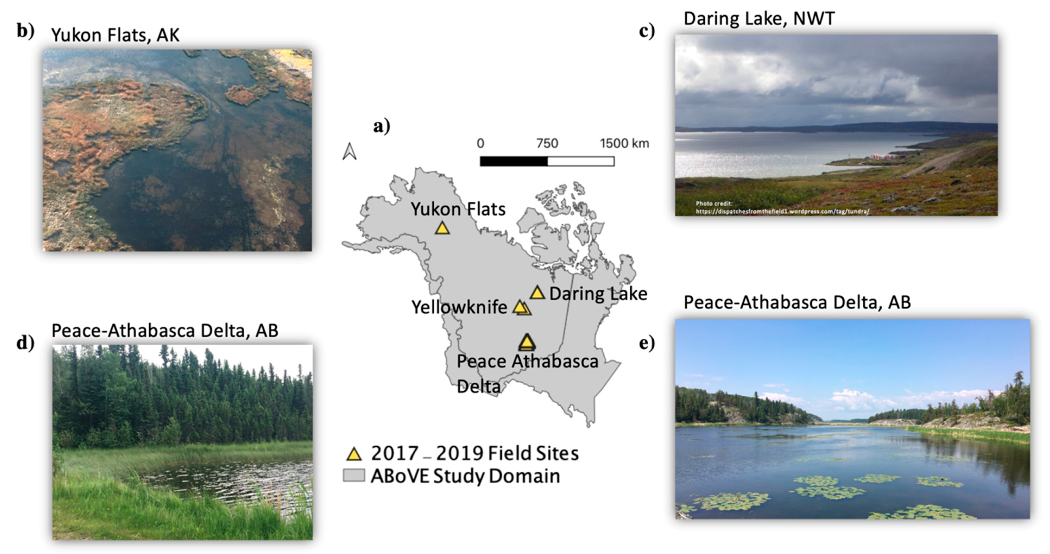
2. Study Lakes
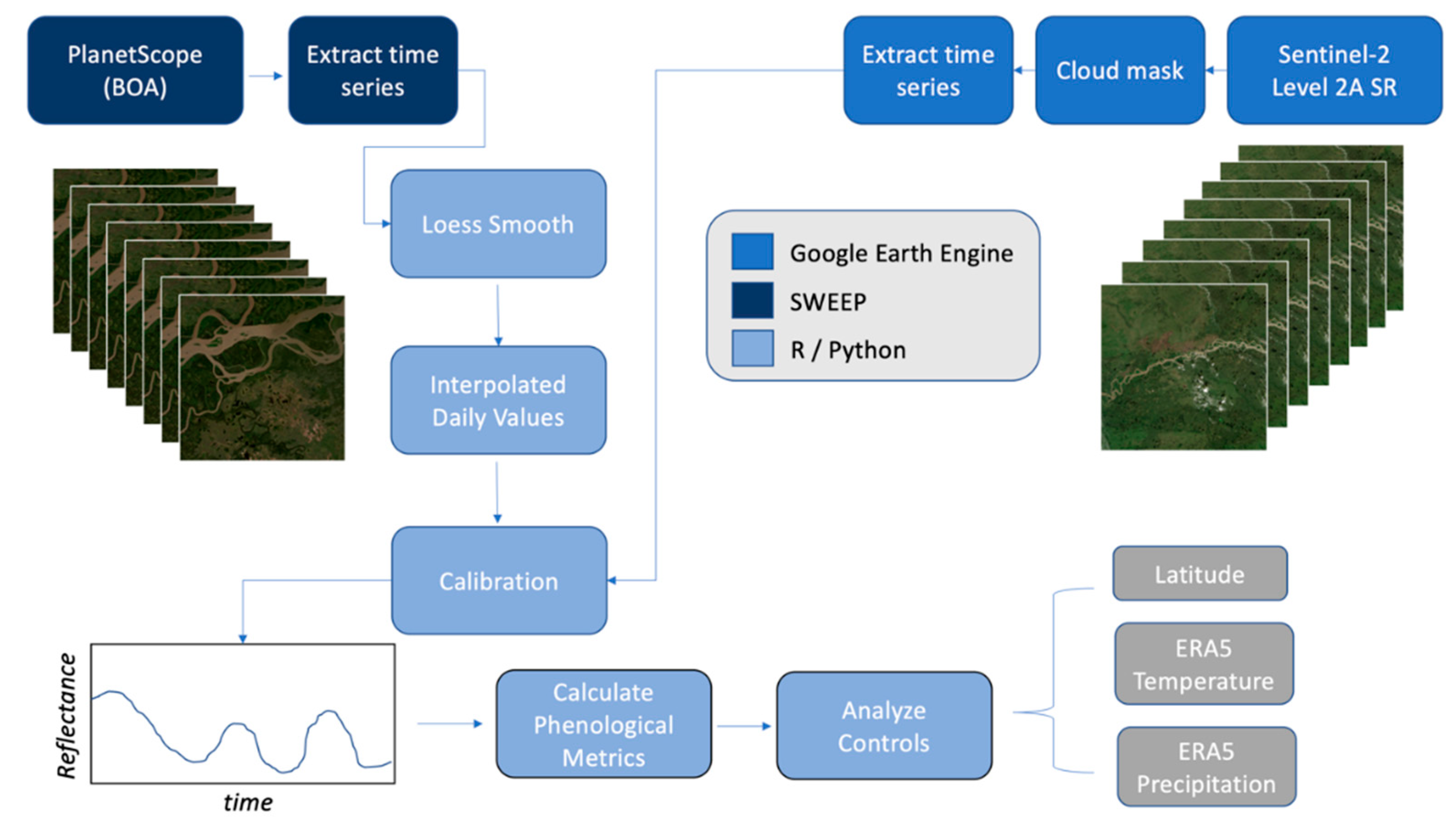
3. Methods
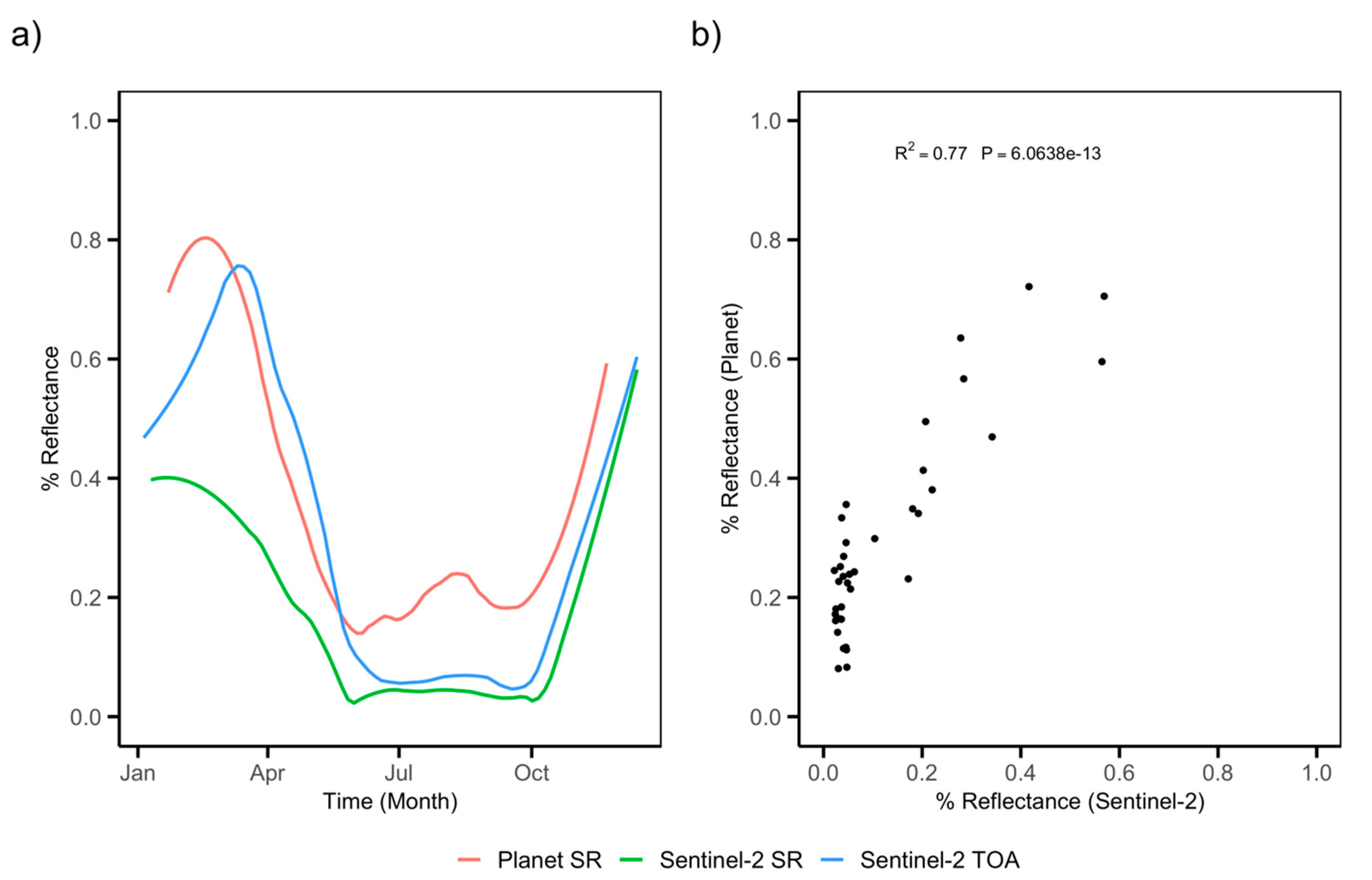
3.1. Satellite Observations
3.2. Time Series Modeling
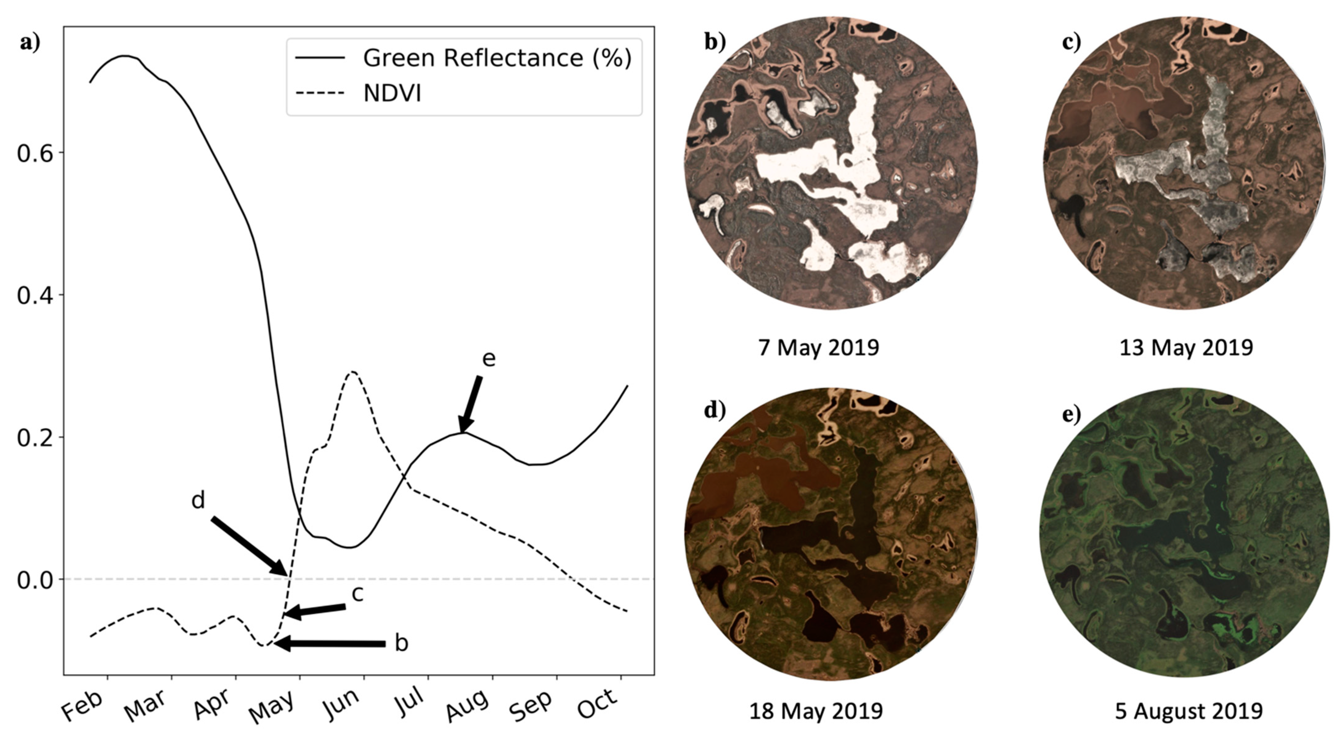
3.3. Phenology Metrics
3.4. Climate Data
3.5. Validation Data
4. Results
4.1. Satellite Imagery Data Quantity and Quality
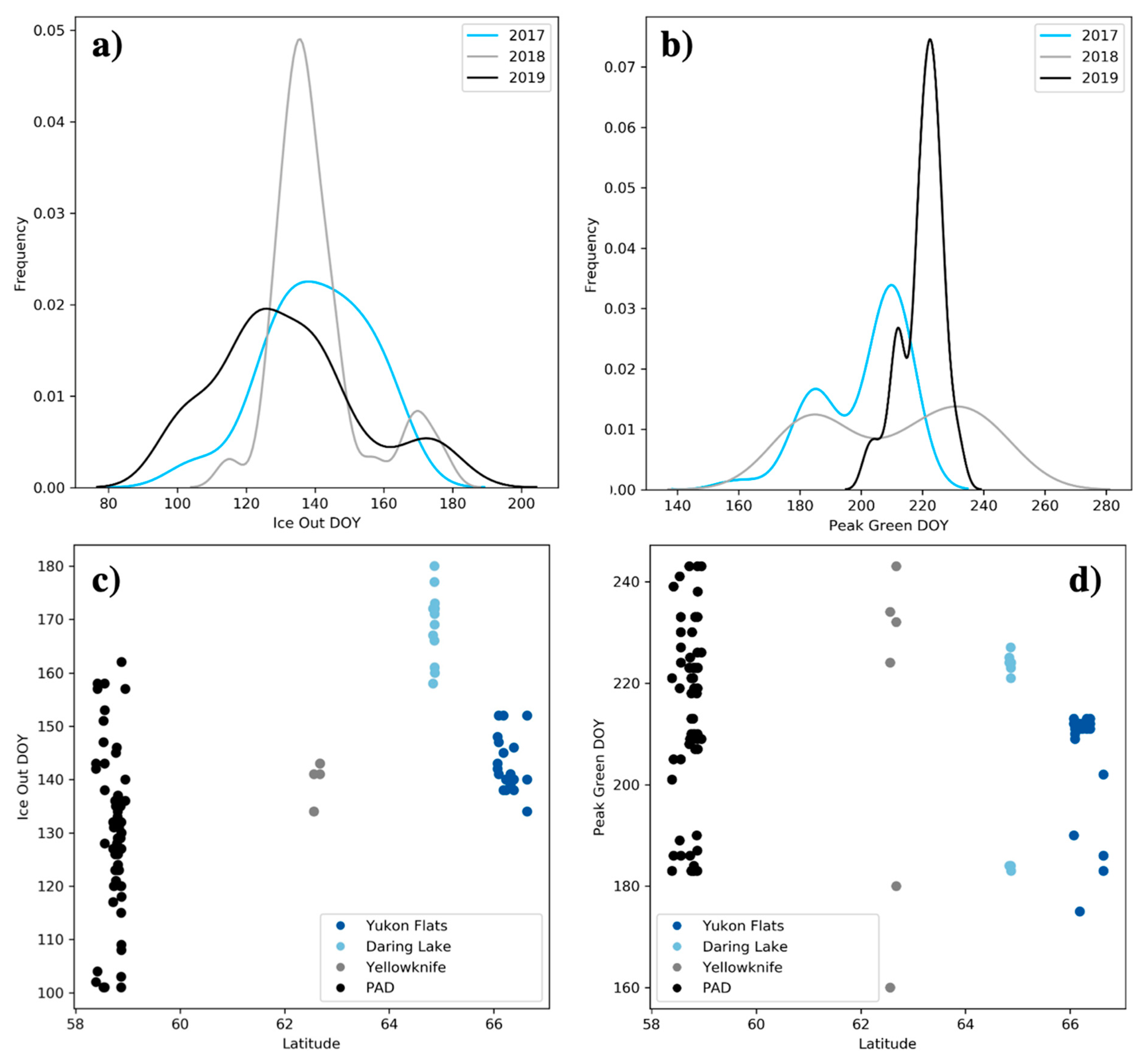
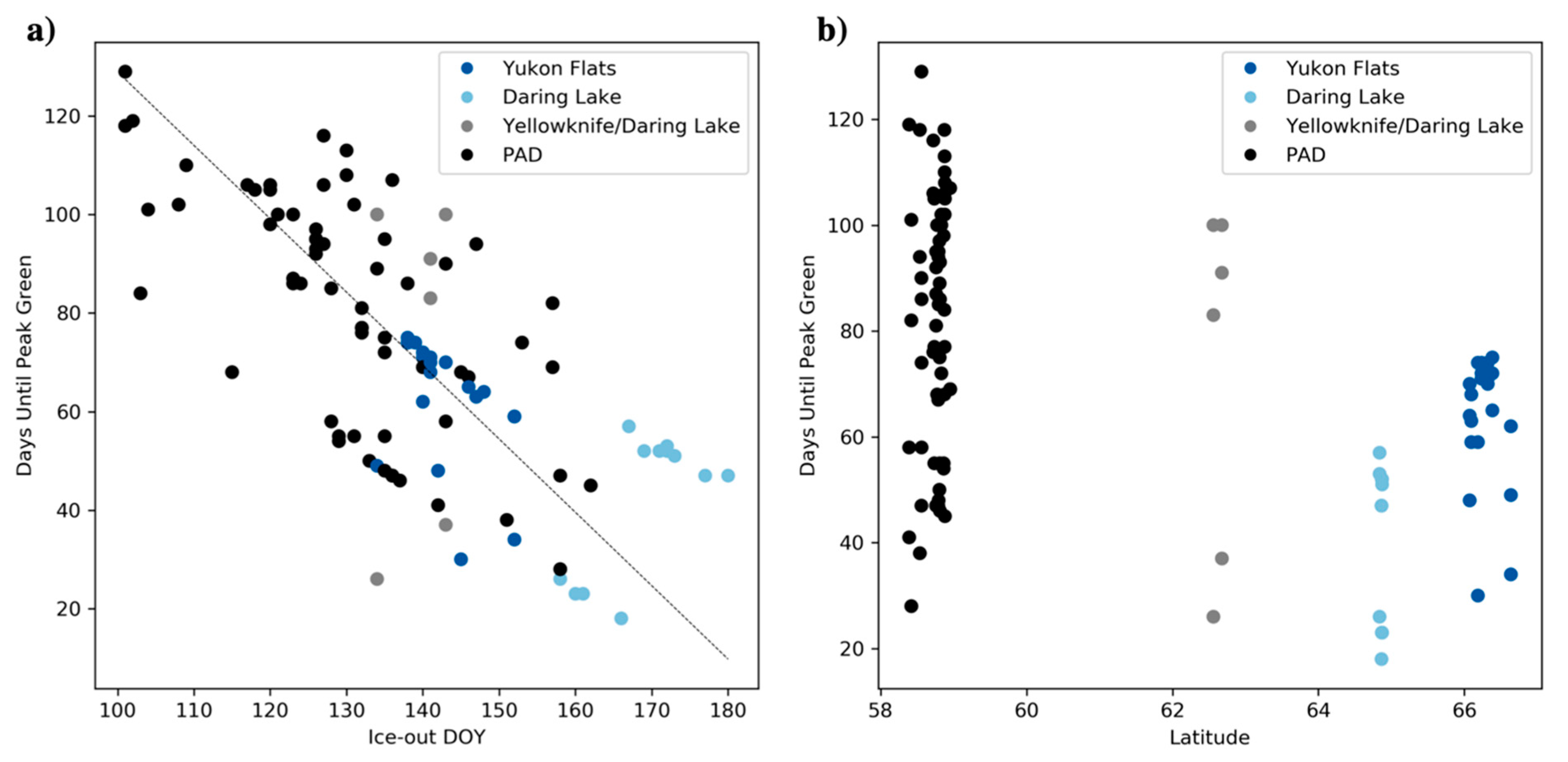
4.2. Phenology Metrics
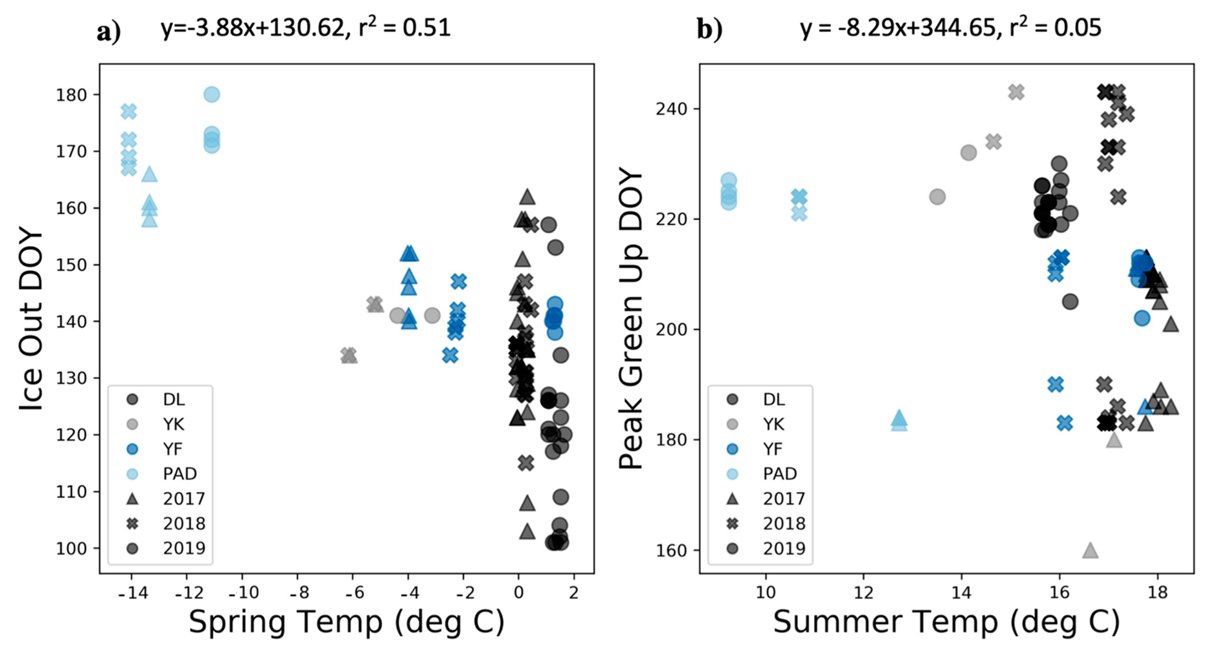
4.3. Climate Patterns and Processes
5. Discussion
5.1. CubeSat Satellites Provide Critical Insight Into Small Lake Ice-Out
5.2. Ice-Out Showed Stronger Coherence with Temperature Than Green-Up
5.3. Future Research Directions
6. Conclusions
Supplementary Materials
Author Contributions
Funding
Data Availability Statement
Acknowledgments
Conflicts of Interest
References
- Downing, J.A.; Prairie, Y.T.; Cole, J.J.; Duarte, C.M.; Tranvik, L.J.; Striegl, R.G.; McDowell, W.H.; Kortelainen, P.; Caraco, N.F.; Melack, J.M. The Global Abundance and Size Distribution of Lakes, Ponds, and Impoundments. Limnol. Oceanogr. 2006, 51, 2388–2397. [Google Scholar] [CrossRef] [Green Version]
- Verpoorter, C.; Kutser, T.; Seekell, D.A.; Tranvik, L.J. A Global Inventory of Lakes Based on High-resolution Satellite Imagery. Geophys. Res. Lett. 2014, 41, 6396–6402. [Google Scholar] [CrossRef]
- Overland, J.E.; Hanna, E.; Hanssen-Bauer, I.; Kim, S.-J.; Walsh, J.E.; Wang, M.; Bhatt, U.S.; Thoman, R.L. Surface Air Temperature. Arct. Rep. Card 2018. [Google Scholar]
- Sharma, S.; Blagrave, K.; Magnuson, J.J.; O’Reilly, C.M.; Oliver, S.; Batt, R.D.; Magee, M.R.; Straile, D.; Weyhenmeyer, G.A.; Winslow, L. Widespread Loss of Lake Ice around the Northern Hemisphere in a Warming World. Nat. Clim. Chang. 2019, 9, 227. [Google Scholar] [CrossRef]
- Adrian, R.; O’Reilly, C.M.; Zagarese, H.; Baines, S.B.; Hessen, D.O.; Keller, W.; Livingstone, D.M.; Sommaruga, R.; Straile, D.; Van Donk, E.; et al. Lakes as Sentinels of Climate Change. Limnol. Oceanogr. 2009, 54, 2283–2297. [Google Scholar] [CrossRef] [PubMed]
- Prowse, T.; Alfredsen, K.; Beltaos, S.; Bonsal, B.; Duguay, C.; Korhola, A.; McNamara, J.; Pienitz, R.; Vincent, W.F.; Vuglinsky, V. Past and Future Changes in Arctic Lake and River Ice. Ambio 2011, 40, 53–62. [Google Scholar] [CrossRef] [Green Version]
- Michelutti, N.; Wolfe, A.P.; Vinebrooke, R.D.; Rivard, B.; Briner, J.P. Recent Primary Production Increases in Arctic Lakes. Geophys. Res. Lett. 2005, 32. [Google Scholar] [CrossRef]
- Woolway, R.I.; Kraemer, B.M.; Lenters, J.D.; Merchant, C.J.; O’Reilly, C.M.; Sharma, S. Global Lake Responses to Climate Change. Nat. Rev. Earth Environ. 2020, 1, 388–403. [Google Scholar] [CrossRef]
- Šmejkalová, T.; Edwards, M.E.; Dash, J. Arctic Lakes Show Strong Decadal Trend in Earlier Spring Ice-Out. Sci. Rep. 2016, 6, 38449. [Google Scholar] [CrossRef] [PubMed]
- Williams, S.G.; Stefan, H.G. Modeling of Lake Ice Characteristics in North America Using Climate, Geography, and Lake Bathymetry. J. Cold Reg. Eng. 2006, 20, 140–167. [Google Scholar] [CrossRef]
- Livingstone, D.M. Break-up Dates of Alpine Lakes as Proxy Data for Local and Regional Mean Surface Air Temperatures. Clim. Chang. 1997, 37, 407–439. [Google Scholar] [CrossRef] [Green Version]
- Prowse, T.; Alfredsen, K.; Beltaos, S.; Bonsal, B.R.; Bowden, W.B.; Duguay, C.R.; Korhola, A.; McNamara, J.; Vincent, W.F.; Vuglinsky, V. Effects of Changes in Arctic Lake and River Ice. Ambio 2011, 40, 63–74. [Google Scholar] [CrossRef] [Green Version]
- Woolway, R.I.; Merchant, C.J. Worldwide Alteration of Lake Mixing Regimes in Response to Climate Change. Nat. Geosci. 2019, 12, 271–276. [Google Scholar] [CrossRef]
- Melles, M.; Brigham-Grette, J.; Glushkova, O.Y.; Minyuk, P.S.; Nowaczyk, N.R.; Hubberten, H.-W. Sedimentary Geochemistry of Core PG1351 from Lake El’gygytgyn—A Sensitive Record of Climate Variability in the East Siberian Arctic during the Past Three Glacial–Interglacial Cycles. J. Paleolimnol. 2007, 37, 89–104. [Google Scholar] [CrossRef]
- Maeda, E.E.; Lisboa, F.; Kaikkonen, L.; Kallio, K.; Koponen, S.; Brotas, V.; Kuikka, S. Temporal Patterns of Phytoplankton Phenology across High Latitude Lakes Unveiled by Long-Term Time Series of Satellite Data. Remote Sens. Environ. 2019, 221, 609–620. [Google Scholar] [CrossRef]
- Guo, M.; Zhuang, Q.; Tan, Z.; Shurpali, N.; Juutinen, S.; Kortelainen, P.; Martikainen, P.J. Rising Methane Emissions from Boreal Lakes Due to Increasing Ice-Free Days. Environ. Res. Lett. 2020, 15, 064008. [Google Scholar] [CrossRef]
- Peeters, F.; Straile, D.; Lorke, A.; Livingstone, D.M. Earlier Onset of the Spring Phytoplankton Bloom in Lakes of the Temperate Zone in a Warmer Climate. Glob. Chang. Biol. 2007, 13, 1898–1909. [Google Scholar] [CrossRef] [Green Version]
- Fritz, S.C.; Anderson, N.J. The Relative Influences of Climate and Catchment Processes on Holocene Lake Development in Glaciated Regions. J. Paleolimnol. 2013, 49, 349–362. [Google Scholar] [CrossRef] [Green Version]
- Ho, J.C.; Michalak, A.M.; Pahlevan, N. Widespread Global Increase in Intense Lake Phytoplankton Blooms since the 1980s. Nature 2019, 574, 667–670. [Google Scholar] [CrossRef]
- Sayers, M.; Bosse, K.; Fahnenstiel, G.; Shuchman, R. Carbon Fixation Trends in Eleven of the World’s Largest Lakes: 2003–2018. Water 2020, 12, 3500. [Google Scholar] [CrossRef]
- Drusch, M.; Del Bello, U.; Carlier, S.; Colin, O.; Fernandez, V.; Gascon, F.; Hoersch, B.; Isola, C.; Laberinti, P.; Martimort, P.; et al. Sentinel-2: ESA’s Optical High-Resolution Mission for GMES Operational Services. Remote Sens. Environ. 2012, 120, 25–36. [Google Scholar] [CrossRef]
- Planet. Planet Application Program Interface. In Space for Life on Earth; Planet: San Francisco, CA, USA, 2017. [Google Scholar]
- Pahlevan, N.; Chittimalli, S.K.; Balasubramanian, S.V.; Vellucci, V. Sentinel-2/Landsat-8 Product Consistency and Implications for Monitoring Aquatic Systems. Remote Sens. Environ. 2019, 220, 19–29. [Google Scholar] [CrossRef]
- Kuhn, C.; Bogard, M.; Johnston, S.E.; John, A.; Vermote, E.F.; Spencer, R.; Dornblaser, M.; Wickland, K.P.; Striegl, R.G.; Butman, D. Satellite and Airborne Remote Sensing of Gross Primary Productivity in Boreal Alaskan Lakes. Environ. Res. Lett. 2020, 15, 105001. [Google Scholar] [CrossRef]
- Poursanidis, D.; Traganos, D.; Chrysoulakis, N.; Reinartz, P. Cubesats Allow High Spatiotemporal Estimates of Satellite-Derived Bathymetry. Remote Sens. 2019, 11, 1299. [Google Scholar] [CrossRef] [Green Version]
- Cheng, Y.; Vrieling, A.; Fava, F.; Meroni, M.; Marshall, M.; Gachoki, S. Phenology of Short Vegetation Cycles in a Kenyan Rangeland from PlanetScope and Sentinel-2. Remote Sens. Environ. 2020, 248, 112004. [Google Scholar] [CrossRef]
- Wulder, M.A.; White, J.C.; Loveland, T.R.; Woodcock, C.E.; Belward, A.; Cohen, W.B. The Global Observing System for Climate: Implementation Needs. In GCOS Implementation Plan GCOS-200 (GOOS-214); World Meteorological Organization: Geneva, Switzerland, 2016. [Google Scholar]
- Cooley, S.W.; Smith, L.C.; Stepan, L.; Mascaro, J. Tracking Dynamic Northern Surface Water Changes with High-Frequency Planet CubeSat Imagery. Remote Sens. 2017, 9, 1306. [Google Scholar] [CrossRef] [Green Version]
- Niroumand-Jadidi, M.; Bovolo, F.; Bruzzone, L.; Gege, P. Physics-Based Bathymetry and Water Quality Retrieval Using Planetscope Imagery: Impacts of 2020 Covid-19 Lockdown and 2019 Extreme Flood in the Venice Lagoon. Remote Sens. 2020, 12, 2381. [Google Scholar] [CrossRef]
- Gabr, B.; Ahmed, M.; Marmoush, Y. PlanetScope and Landsat 8 Imageries for Bathymetry Mapping. J. Mar. Sci. Eng. 2020, 8, 143. [Google Scholar] [CrossRef] [Green Version]
- Wirabumi, P.; Wicaksono, P.; Kamal, M.; Ridwansyah, I.; Subehi, L.; Dianto, A. Spatial Distribution Analysis of Total Suspended Solid (TSS) Using PlanetScope Data in Menjer Lake, Wonosobo Regency. Geospat. Inf. 2020, 4. [Google Scholar] [CrossRef]
- Vanhellemont, Q. Daily Metre-Scale Mapping of Water Turbidity Using CubeSat Imagery. Opt. Express 2019, 27, A1372–A1399. [Google Scholar] [CrossRef]
- Warner, K.A.; Fowler, R.A.; Northington, R.M.; Malik, H.I.; McCue, J.; Saros, J.E. How Does Changing Ice-out Affect Arctic versus Boreal Lakes? A Comparison Using Two Years with Ice-out That Differed by More than Three Weeks. Water 2018, 10, 78. [Google Scholar] [CrossRef] [Green Version]
- Saros, J.E.; Anderson, N.J.; Juggins, S.; McGowan, S.; Yde, J.C.; Telling, J.; Bullard, J.E.; Yallop, M.L.; Heathcote, A.J.; Burpee, B.T. Arctic Climate Shifts Drive Rapid Ecosystem Responses across the West Greenland Landscape. Environ. Res. Lett. 2019, 14, 74027. [Google Scholar] [CrossRef]
- Planet. Planet Surface Reflectance 2.0. 2020. Available online: https://assets.planet.com/marketing/PDF/Planet_Surface_Reflectance_Technical_White_Paper.pdf (accessed on 27 June 2021).
- John, A.; Ausmees, K.; Muenzen, K.; Kuhn, C.; Tan, A. SWEEP: Accelerating Scientific Research through Scalable Serverless Workflows. In Proceedings of the UCC ’19 Companion: IEEE/ACM 12th International Conference on Utility and Cloud Computing Companion, Auckland, New Zealand, 2–5 December 2019. [Google Scholar]
- Gorelick, N.; Hancher, M.; Dixon, M.; Ilyushchenko, S.; Thau, D.; Moore, R. Google Earth Engine: Planetary-Scale Geospatial Analysis for Everyone. Remote Sens. Environ. 2017, 202, 18–27. [Google Scholar] [CrossRef]
- Kuhn, C.; de Matos Valerio, A.; Ward, N.; Loken, L.; Sawakuchi, H.O.; Kampel, M.; Richey, J.; Stadler, P.; Crawford, J.; Striegl, R.; et al. Performance of Landsat-8 and Sentinel-2 Surface Reflectance Products for River Remote Sensing Retrievals of Chlorophyll-a and Turbidity. Remote Sens. Environ. 2019, 224, 104–118. [Google Scholar] [CrossRef] [Green Version]
- Main-Knorn, M.; Pflug, B.; Louis, J.; Debaecker, V.; Müller-Wilm, U.; Gascon, F. Sen2Cor for Sentinel-2. In Proceedings of the Image and Signal Processing for Remote Sensing XXIII, Warsaw, Poland, 11–13 September 2017; Volume 10427, p. 1042704. [Google Scholar]
- Cleveland, W.S.; Grosse, E. Computational Methods for Local Regression. Stat. Comput. 1991, 1, 47–62. [Google Scholar] [CrossRef]
- Tucker, C.J. Red and Photographic Infrared Linear Combinations for Monitoring Vegetation. Remote Sens. Environ. 1979, 8, 127–150. [Google Scholar] [CrossRef] [Green Version]
- Pettorelli, N.; Vik, J.O.; Mysterud, A.; Gaillard, J.-M.; Tucker, C.J.; Stenseth, N.C. Using the Satellite-Derived NDVI to Assess Ecological Responses to Environmental Change. Trends Ecol. Evol. 2005, 20, 503–510. [Google Scholar] [CrossRef] [PubMed]
- Hollingsworth, T.; Baird, R.A.; Verbyla, D.; Hollingsworth, T.N. Browning of the Landscape of Interior Alaska Based on 1986-2009 Landsat Sensor NDVI. Can. J. For. Res. 2012, 42, 1371–1382. [Google Scholar]
- Bhatt, U.; Walker, D.; Raynolds, M.; Bieniek, P.; Epstein, H.; Comiso, J.; Pinzon, J.; Tucker, C.; Polyakov, I.; Bhatt, U.S.; et al. Recent Declines in Warming and Vegetation Greening Trends over Pan-Arctic Tundra. Remote Sens. 2013, 5, 4229–4254. [Google Scholar] [CrossRef] [Green Version]
- Morel, A.; Prieur, L. Analysis of Variations in Ocean Color. Limnol. Oceanogr. 1977, 22, 709–722. [Google Scholar] [CrossRef]
- Zhang, B.; Li, J.; Shen, Q.; Chen, D. A Bio-Optical Model Based Method of Estimating Total Suspended Matter of Lake Taihu from near-Infrared Remote Sensing Reflectance. Environ. Monit. Assess. 2008, 145, 339–347. [Google Scholar] [CrossRef] [PubMed]
- Gitelson, A.A.; Schalles, J.F.; Hladik, C.M. Remote Chlorophyll-a Retrieval in Turbid, Productive Estuaries: Chesapeake Bay Case Study. Remote Sens. Environ. 2007, 109, 464–472. [Google Scholar] [CrossRef]
- Kallio, K.; Kutser, T.; Hannonen, T.; Koponen, S.; Pulliainen, J.; Vepsäläinen, J.; Pyhälahti, T. Retrieval of Water Quality from Airborne Imaging Spectrometry of Various Lake Types in Different Seasons. Sci. Total Environ. 2001, 268, 59–77. [Google Scholar] [CrossRef]
- Zhang, Y.; Lin, H.; Chen, C.; Chen, L.; Zhang, B.; Gitelson, A.A. Estimation of Chlorophyll-a Concentration in Estuarine Waters: Case Study of the Pearl River Estuary, South China Sea. Environ. Res. Lett. 2011, 6, 24016. [Google Scholar] [CrossRef]
- Wang, M.; Shi, W. Estimation of Ocean Contribution at the MODIS Near-infrared Wavelengths along the East Coast of the US: Two Case Studies. Geophys. Res. Lett. 2005, 32. [Google Scholar] [CrossRef] [Green Version]
- Kutser, T. Quantitative Detection of Chlorophyll in Cyanobacterial Blooms by Satellite Remote Sensing. Limnol. Oceanogr. 2004, 49, 2179–2189. [Google Scholar] [CrossRef]
- Hunter, P.D.; Gilvear, D.J.; Tyler, A.N.; Willby, N.J.; Kelly, A. Mapping Macrophytic Vegetation in Shallow Lakes Using the Compact Airborne Spectrographic Imager (CASI). Aquat. Conserv. Mar. Freshw. Ecosyst. 2010, 20, 717–727. [Google Scholar] [CrossRef]
- Dogan, O.K.; Akyurek, Z.; Beklioglu, M. Identification and Mapping of Submerged Plants in a Shallow Lake Using Quickbird Satellite Data. J. Environ. Manag. 2009, 90, 2138–2143. [Google Scholar] [CrossRef]
- Bresciani, M.; Sotgia, C.; Fila, G.L.; Musanti, M.; Bolpagni, R. Assessing Common Reed Bed Health and Management Strategies in Lake Garda (Italy) by Means of Leaf Area Index Measurements. Ital. J. Remote Sens. 2011, 43, 9–22. [Google Scholar] [CrossRef]
- Campbell, J.B.; Wynne, R.H. Introduction to Remote Sensing; Guilford Press: New York, NY, USA, 2011; ISBN 1-60918-177-8. [Google Scholar]
- Gitelson, A. Algorithms for Remote Sensing of Phytoplankton Pigments in Inland Waters. Adv. Space Res. 1993, 13, 197–201. [Google Scholar] [CrossRef]
- Schalles, J.F. Optical Remote Sensing Techniques to Estimate Phytoplankton Chlorophyll a Concentrations in Coastal. In Remote Sensing of Aquatic Coastal Ecosystem Processes; Springer: Dordrecht, The Netherlands, 2006; pp. 27–79. [Google Scholar]
- Fahnenstiel, G.L.; Sayers, M.J.; Shuchman, R.A.; Yousef, F.; Pothoven, S.A. Lake-Wide Phytoplankton Production and Abundance in the Upper Great Lakes: 2010–2013. J. Great Lakes Res. 2016, 42, 619–629. [Google Scholar] [CrossRef]
- Urraca, R.; Huld, T.; Gracia-Amillo, A.; Martinez-de-Pison, F.J.; Kaspar, F.; Sanz-Garcia, A. Evaluation of Global Horizontal Irradiance Estimates from ERA5 and COSMO-REA6 Reanalyses Using Ground and Satellite-Based Data. Sol. Energy 2018, 164, 339–354. [Google Scholar] [CrossRef]
- Albergel, C.; Dutra, E.; Munier, S.; Calvet, J.-C.; Munoz-Sabater, J.; Rosnay, P.D.; Balsamo, G. ERA-5 and ERA-Interim Driven ISBA Land Surface Model Simulations: Which One Performs Better? Hydrol. Earth Syst. Sci. 2018, 22, 3515–3532. [Google Scholar] [CrossRef] [Green Version]
- Giardino, C.; Brando, V.E.; Gege, P.; Pinnel, N.; Hochberg, E.; Knaeps, E.; Reusen, I.; Doerffer, R.; Bresciani, M.; Braga, F.; et al. Imaging Spectrometry of Inland and Coastal Waters: State of the Art, Achievements and Perspectives. Surv. Geophys. 2018, 40, 1–29. [Google Scholar] [CrossRef] [Green Version]
- Lafleur, P.M.; Humphreys, E.R. Spring Warming and Carbon Dioxide Exchange over Low Arctic Tundra in Central Canada: Spring warming and arctic tundra CO2 exchange. Glob. Chang. Biol. 2008, 14, 740–756. [Google Scholar] [CrossRef]
- Walvoord, M.A.; Voss, C.I.; Wellman, T.P. Influence of Permafrost Distribution on Groundwater Flow in the Context of Climate-Driven Permafrost Thaw: Example from Yukon Flats Basin, Alaska, United States: Permafrost distribution and groundwater flow. Water Resour. Res. 2012, 48. [Google Scholar] [CrossRef]
- Higgins, S.N.; Desjardins, C.M.; Drouin, H.; Hrenchuk, L.E.; van der Sanden, J.J. The Role of Climate and Lake Size in Regulating the Ice Phenology of Boreal Lakes. J. Geophys. Res. Biogeosci. 2021, 126, e2020JG005898. [Google Scholar] [CrossRef]
- Nicolle, A.; Hallgren, P.; Von EINEM, J.; Kritzberg, E.S.; Granéli, W.; Persson, A.; Brönmark, C.; Hansson, L.-A. Predicted Warming and Browning Affect Timing and Magnitude of Plankton Phenological Events in Lakes: A Mesocosm Study: Temperature, Water Colour and Plankton. Freshw. Biol. 2012, 57, 684–695. [Google Scholar] [CrossRef]
- Houborg, R.; McCabe, M.F. A Cubesat Enabled Spatio-Temporal Enhancement Method (Cestem) Utilizing Planet, Landsat and Modis Data. Remote Sens. Environ. 2018, 209, 211–226. [Google Scholar] [CrossRef]
- Li, Z.; Zhang, H.K.; Roy, D.P.; Yan, L.; Huang, H. Sharpening the Sentinel-2 10 and 20 m Bands to Planetscope-0 3 m Resolution. Remote Sens. 2020, 12, 2406. [Google Scholar] [CrossRef]
- Arp, C.D.; Jones, B.M.; Grosse, G. Recent Lake Ice-out Phenology within and among Lake Districts of Alaska, USA. Limnol. Oceanogr. 2013, 58, 2013–2028. [Google Scholar] [CrossRef]
- Palecki, M.A.; Barry, R.G. Freeze-up and Break-up of Lakes as an Index of Temperature Changes during the Transition Seasons: A Case Study for Finland. J. Appl. Meteorol. Climatol. 1986, 25, 893–902. [Google Scholar] [CrossRef]
- Robertson, D.M.; Ragotzkie, R.A.; Magnuson, J.J. Lake Ice Records Used to Detect Historical and Future Climatic Changes. Clim. Chang. 1992, 21, 407–427. [Google Scholar] [CrossRef]
- Preston, D.L.; Caine, N.; McKnight, D.M.; Williams, M.W.; Hell, K.; Miller, M.P.; Hart, S.J.; Johnson, P.T.J. Climate Regulates Alpine Lake Ice Cover Phenology and Aquatic Ecosystem Structure. Geophys. Res. Lett. 2016, 43, 5353–5360. [Google Scholar] [CrossRef]
- Pavelsky, T.M.; Smith, L.C. Remote Sensing of Hydrologic Recharge in the Peace-Athabasca Delta, Canada. Geophys. Res. Lett. 2008, 35. [Google Scholar] [CrossRef] [Green Version]
- Peters, D.L.; Prowse, T.D.; Pietroniro, A.; Leconte, R. Flood Hydrology of the Peace-Athabasca Delta, Northern Canada. Hydrol. Process. Int. J. 2006, 20, 4073–4096. [Google Scholar] [CrossRef]
- Wolfe, B.B.; Hall, R.I.; Wiklund, J.A.; Kay, M.L. Past Variation in Lower Peace River Ice-Jam Flood Frequency. Environ. Rev. 2020, 28, 209–217. [Google Scholar] [CrossRef] [Green Version]
- Sheath, R.G. Seasonality of Phytoplankton in Northern Tundra Ponds. Hydrobiologia 1986, 138, 75–83. [Google Scholar] [CrossRef]
- Peltomaa, E.; Ojala, A.; Holopainen, A.-L.; Salonen, K. Changes in Phytoplankton in a Boreal Lake during a 14-Year Period. Boreal Environ. Res. 2013, 18, 387–400. [Google Scholar]
- Rühland, K.; Paterson, A.M.; Smol, J.P. Hemispheric-scale Patterns of Climate-related Shifts in Planktonic Diatoms from North American and European Lakes. Glob. Chang. Biol. 2008, 14, 2740–2754. [Google Scholar] [CrossRef]
- R Development Core Team. A Language and Environment for Statistical Computing: Reference Index; R Foundation for Statistical Computing: Vienna, Austria, 2010; ISBN 978-3-900051-07-5. [Google Scholar]
- Wickham, H. Package Tidyverse. Easily Install and Load the ‘Tidyverse. 2017. Available online: http://ftp.gr.xemacs.org/pub/CRAN/web/packages/tidyverse/tidyverse.pdf (accessed on 27 June 2021).


| SiteName | Location | Latitude | Longitude | Area | Depth |
|---|---|---|---|---|---|
| Daring Lake | Daring Lake | 64.86505 | −111.59285 | 332.7 | 3 |
| Daring Lake 4 | Daring Lake | 64.8387 | −111.5878 | 0.043 | 1.5 |
| Esker Lake 1 | Daring Lake | 64.86983 | −111.55095 | 0.1 | 1 |
| Lake 10 near Yellowknife | Yellowknife | 62.67747 | −115.37342 | 0.036 | 4.4 |
| Lake Kakawi | Daring Lake | 64.87323 | −111.58733 | 0.026 | 2.8 |
| Lake M2 near Yellowknife | Yellowknife | 62.56125 | −114.02278 | 0.019 | 1.5 |
| Balloon Lake (No.0) | Peace Athabasca Delta | 58.87754 | −111.22644 | 0.04 | 2 |
| Balloon Lake #1 | Peace Athabasca Delta | 58.87856 | −111.25269 | 0.036 | 0.6 |
| Big Beaver | Peace Athabasca Delta | 58.76115 | −111.08667 | 0.14 | 3.1 |
| Blanche | Peace Athabasca Delta | 58.39219 | −111.27903 | 4.16 | 1.8 |
| Chillowe’s Lake | Peace Athabasca Delta | 58.82465 | −111.36208 | 0.24 | 4.2 |
| Dore Lake | Peace Athabasca Delta | 58.79043 | −111.0497 | 0.79 | 5.6 |
| Egg Lake | Peace Athabasca Delta | 58.88345 | −111.40038 | 0.053 | 0.3 |
| Emberras Pond | Peace Athabasca Delta | 58.55952 | −111.16557 | 9.4 | 1.3 |
| Flett Lake | Peace Athabasca Delta | 58.95387 | −111.0783 | 1.31 | 4.1 |
| Green Star Lake | Peace Athabasca Delta | 58.89665 | −111.36157 | 0.79 | 4.6 |
| High Lake | Peace Athabasca Delta | 58.79609 | −111.03199 | 0.06 | 1 |
| Horseshoe | Peace Athabasca Delta | 58.86379 | −111.58447 | 0.31 | 0.8 |
| Limon | Peace Athabasca Delta | 58.42109 | −111.31567 | 6.79 | 1.5 |
| Little Beaver | Peace Athabasca Delta | 58.76194 | −111.08722 | 0.041 | 5.5 |
| Little Lake | Peace Athabasca Delta | 58.73637 | −111.12198 | 0.52 | 5.8 |
| Long Lake | Peace Athabasca Delta | 58.53797 | −111.48681 | 1.11 | 0.9 |
| PAD3 | Peace Athabasca Delta | 58.56163 | −111.50293 | 1 | 1.4 |
| Rat Lake | Peace Athabasca Delta | 58.87465 | −111.32388 | 0.003 | 0.6 |
| Robert’s Cabin Pond | Peace Athabasca Delta | 58.8057 | −111.24348 | 0.14 | 1.25 |
| Roche Pond | Peace Athabasca Delta | 58.83302 | −111.28278 | 0.1 | 0.8 |
| Swan’s Fly Farm Pond | Peace Athabasca Delta | 58.72254 | −111.19344 | 0.02 | 0.5 |
| Third Lake | Peace Athabasca Delta | 58.77452 | −111.09328 | 1.85 | 4.5 |
| Boot | Yukon Flats | 66.07404 | −146.27066 | 0.73 | 22 |
| Canvasback Lake | Yukon Flats | 66.38303 | −146.35489 | 2.83 | 1.4 |
| Greenpepper Lake | Yukon Flats | 66.09209 | −146.73557 | 0.97 | 10.3 |
| Ninemile | Yukon Flats | 66.18285 | −146.66376 | 3.33 | 1.8 |
| Scoter | Yukon Flats | 66.24241 | −146.39896 | 4.56 | 4.5 |
| YF17 | Yukon Flats | 66.32072 | −146.27431 | 1.75 | 1.6 |
| YF20 | Yukon Flats | 66.63715 | −145.77278 | 0.59 | 1.25 |
Publisher’s Note: MDPI stays neutral with regard to jurisdictional claims in published maps and institutional affiliations. |
© 2021 by the authors. Licensee MDPI, Basel, Switzerland. This article is an open access article distributed under the terms and conditions of the Creative Commons Attribution (CC BY) license (https://creativecommons.org/licenses/by/4.0/).
Share and Cite
Kuhn, C.; John, A.; Hille Ris Lambers, J.; Butman, D.; Tan, A. Arctic-Boreal Lake Phenology Shows a Relationship between Earlier Lake Ice-Out and Later Green-Up. Remote Sens. 2021, 13, 2533. https://0-doi-org.brum.beds.ac.uk/10.3390/rs13132533
Kuhn C, John A, Hille Ris Lambers J, Butman D, Tan A. Arctic-Boreal Lake Phenology Shows a Relationship between Earlier Lake Ice-Out and Later Green-Up. Remote Sensing. 2021; 13(13):2533. https://0-doi-org.brum.beds.ac.uk/10.3390/rs13132533
Chicago/Turabian StyleKuhn, Catherine, Aji John, Janneke Hille Ris Lambers, David Butman, and Amanda Tan. 2021. "Arctic-Boreal Lake Phenology Shows a Relationship between Earlier Lake Ice-Out and Later Green-Up" Remote Sensing 13, no. 13: 2533. https://0-doi-org.brum.beds.ac.uk/10.3390/rs13132533