
Integration of Satellite InSAR with a Wireless Network of Geotechnical Sensors for Slope Monitoring in Urban Areas: The Pariana Landslide Case (Massa, Italy)

 , ,
, ,
Abstract
:1. Introduction
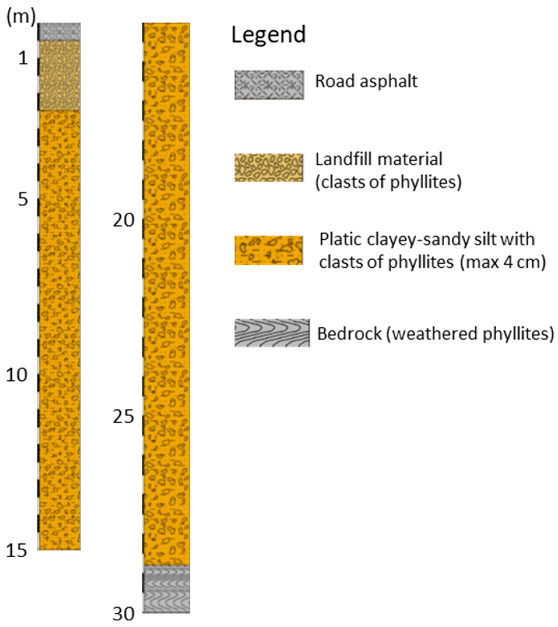
2. Study Area
3. Materials and Methods
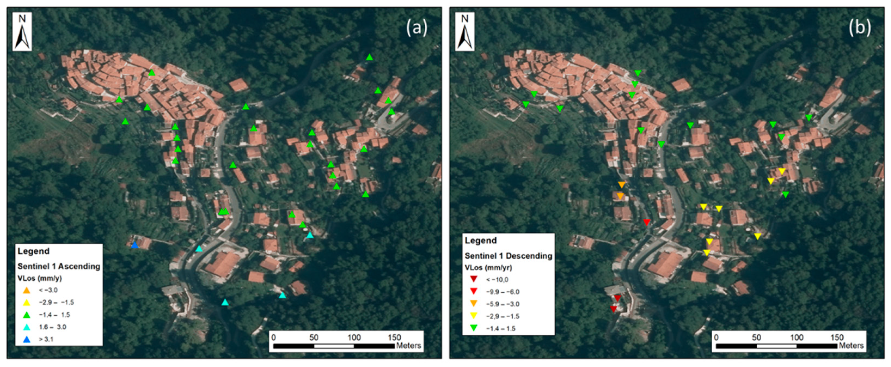
3.1. InSAR Data
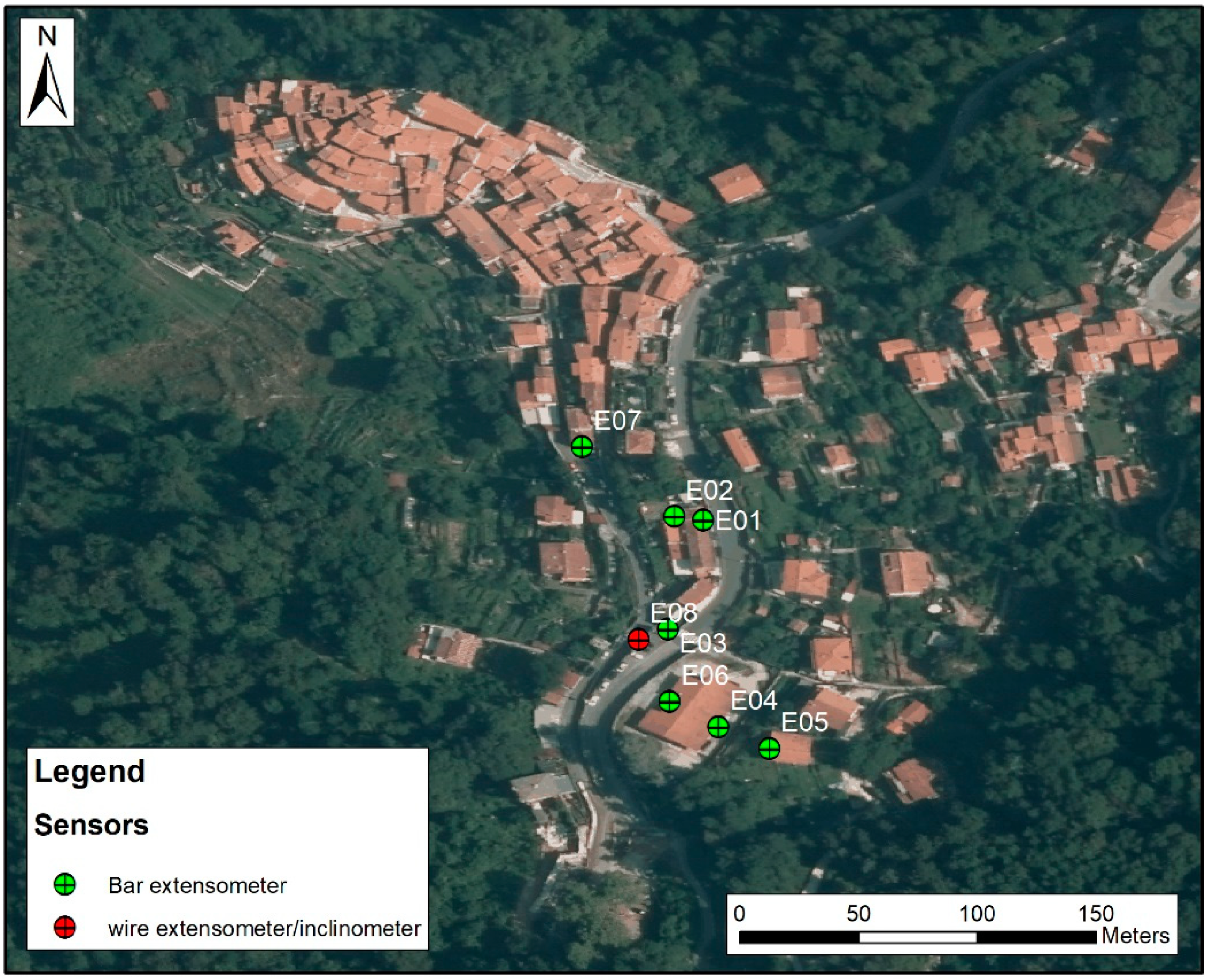
3.2. Geotechnical Monitoring Network
3.3. Integration
4. Results
5. Discussion
6. Conclusions
Author Contributions
Funding
Institutional Review Board Statement
Informed Consent Statement
Data Availability Statement
Acknowledgments
References
- Petley, D. Global patterns of loss of life from landslides. Geology 2012, 40, 927–930. [Google Scholar] [CrossRef]
- Herrera, G.; Mateos, R.M.; Garciá-Davalillo, J.C.; Grandjean, G.; Poyadji, E.; Maftei, R.; Filipciuc, T.-C.; Auflič, M.J.; Jež, J.; Podolszki, L.; et al. Landslide databases in the Geological Surveys of Europe. Landslides 2018, 15, 359–379. [Google Scholar] [CrossRef]
- Codebo, L.; Delmonaco, G.; Margottini, C.; Puglisi, C.; Serafini, S. Landslide susceptibility in the Cardoso slope (Versilia-Italy) consequences of the flash flood of 19 June 1996. In Landslides in Research, Theory and Practice, Proceeding of the 8th International Symp. on Landslides, Cardiff, UK, 26–30 June 2000; Bromhead, E., Dixon, N., Ibsen, M., Eds.; ICE Publishing: London, UK, 2000; Volume 1, pp. 293–298. [Google Scholar]
- Montrasio, M.; Valentino, R.; Losi, G.L. Raifall-induced shallow landslides: A model for the triggering mechanism of some case studies in Northenr Italy. Landslides 2018, 6, 359–379. [Google Scholar] [CrossRef]
- Casagli, N.; Dapporto, S.; Ibsen, M.; Tofani, V.; Vannocci, P. Analysis of the landslide triggering mechanism during the storm of 20–21 November 2000, in Northern Tuscany. Landslides 2006, 3, 13–21. [Google Scholar] [CrossRef]
- Rosi, A.; Segoni, S.; Catani, F.; Casagli, N. Statistical and environmental analyses for the definition of a regional rainfall threshold system for landslide triggering in Tuscany (Italy). J. Geogr. Sci. 2012, 22, 617–629. [Google Scholar] [CrossRef]
- Cruden, D.M.; Varnes, D.J. Landslide type and processes. In Landslides: Investigation and Mitigation, Sp. Rep. 247; Turner, A.K., Schuster, R.L., Eds.; Transportation Research Board, National Research Council, National Academy Press: Washington, DC, USA, 1996; pp. 36–75. [Google Scholar]
- Guzzetti, F. Landslide fatalities and the evaluation of landslide risk in Italy. Eng. Geol. 2000, 58, 89–107. [Google Scholar] [CrossRef]
- Carlini, M.; Chelli, A.; Vescovi, P.; Artoni, A.; Clemenzi, L.; Tellini, C.; Torelli, L. Tectonic control on the development and distribution of large landslides in the Northern Apennines. Geomorphology 2016, 253, 425–437. [Google Scholar] [CrossRef]
- Raspini, F.; Bianchini, S.; Ciampalini, A.; Del Soldato, M.; Montalti, R.; Solari, L.; Tofani, V.; Casagli, N. Persistent Scatterers continuous streaming for landslide monitoring and mapping: The case of the Tuscany region (Italy). Landslides 2019, 16, 2033–2044. [Google Scholar] [CrossRef] [Green Version]
- Del Soldato, M.; Solari, L.; Raspini, F.; Bianchini, S.; Ciampalini, A.; Montalti, R.; Ferretti, A.; Pellegrineschi, V.; Casagli, N. Monitoring Ground Instabilities Using SAR Satellite Data: A Practical Approach. ISPRS Int. J. Geo-Inf. 2019, 8, 307. [Google Scholar] [CrossRef] [Green Version]
- Stark, T.D.; Choi, H. Slope inclinometers for landslides. Landslides 2008, 5, 339. [Google Scholar] [CrossRef]
- Sharon, M.; Eberhardt, E. Guidelines for Slope Performance Monitoring; CRC Press, Taylor & Francis Group: Leiden, The Netherland, 2020. [Google Scholar]
- Li, Y.; Huang, J.; Jiang, S.-H.; Huang, F.; Chang, Z. A web-based GPS system for displacement monitoring and failure mechanism analysis of reservoir landslide. Sci. Rep. 2017, 7, 17171. [Google Scholar] [CrossRef] [Green Version]
- Corominas, J.; Moya, J.; Lloret, A.; Gili, J.; Angeli, M.; Pasuto, A.; Silvano, S. Measurement of landslide displacements using a wire extensometer. Eng. Geol. 2000, 55, 149–166. [Google Scholar] [CrossRef]
- Colesanti, C.; Ferretti, A.; Prati, C.; Rocca, F. Monitoring landslides and tectonic motions with the Permanent Scatterers Technique. Eng. Geol. 2003, 68, 3–14. [Google Scholar] [CrossRef]
- Frodella, W.; Ciampalini, A.; Gigli, G.; Lombardi, L.; Raspini, F.; Nocentini, M.; Scardigli, C.; Casagli, N. Synergic use of satellite and ground based remote sensing methods for monitoring the San Leo rock cliff (Northern Italy). Geomorphology 2016, 264, 80–94. [Google Scholar] [CrossRef]
- Ma, J.; Niu, X.; Liu, X.; Wang, Y.; Wen, T.; Zhang, J. Thermal Infrared Imagery Integrated with Terrestrial Laser Scanning and Particle Tracking Velocimetry for Characterization of Landslide Model Failure. Sensors 2020, 20, 219. [Google Scholar] [CrossRef] [Green Version]
- Lombardi, L.; Nocentini, M.; Frodella, W.; Nolesini, T.; Bardi, F.; Intrieri, E.; Carlà, T.; Solari, L.; Dotta, G.; Ferrigno, F.; et al. The Calatabiano landslide (southern Italy): Preliminary GB-InSAR monitoring data and remote 3D mapping. Landslides 2017, 14, 685–696. [Google Scholar] [CrossRef] [Green Version]
- Darvishi, M.; Schlögel, R.; Kofler, C.; Cuozzo, G.; Rutzinger, M.; Zieher, T.; Toschi, I.; Remondino, F.; Mejia-Aguilar, A.; Thiebes, B.; et al. Sentinel-1 and Ground-Based Sensors for Continuous Monitoring of the Corvara Landslide (South Tyrol, Italy). Remote Sens. 2018, 10, 1781. [Google Scholar] [CrossRef] [Green Version]
- Lan, H.; Zhao, X.; Macciotta, R.; Peng, J.; Li, L.; Wu, Y.; Zhu, Y.; Liu, X.; Zhang, N.; Liu, S.; et al. The cyclic expansion and contraction characteristics of a loess slope and implications for slope stability. Sci. Rep. 2021, 11, 2250. [Google Scholar] [CrossRef] [PubMed]
- Woods, A.; Macciotta, R.; Hendry, M.T.; Stewart, T.; Marsh, J. Updated understanding of the deformation characteristics of the Checkerboard Creek rock slope through GB-InSAR monitoring. Eng. Geol. 2021, 281, 105974. [Google Scholar] [CrossRef]
- Fernández, T.; Pérez, J.L.; Cardenal, J.; Gómez, J.M.; Colomo, C.; Delgado, J. Analysis of Landslide Evolution Affecting Olive Groves Using UAV and Photogrammetric Techniques. Remote Sens. 2016, 8, 837. [Google Scholar] [CrossRef] [Green Version]
- Rossi, G.; Tanteri, L.; Tofani, V.; Vannocci, P.; Moretti, S.; Casagli, N. Multitemporal UAV surveys for landslide mapping and characterization. Landslides 2018, 15, 1045–1052. [Google Scholar] [CrossRef] [Green Version]
- Intrieri, E.; Gigli, G.; Mugnai, F.; Fanti, R.; Casagli, N. Design and implementation of a landslide early warning system. Eng. Geol. 2012, 147–148, 124–136. [Google Scholar] [CrossRef] [Green Version]
- Koha, V.V.; Takayama, S. Wireless sensor network in landslide monitoring system with remote data management. Measurements 2018, 118, 214–229. [Google Scholar]
- Jeong, S.; Ko, J.; Kim, J. The effectiveness of a wireless sensor network system for landslide monitoring. IEEE Access 2020, 8, 8073–8086. [Google Scholar] [CrossRef]
- Singhroy, V.; Mattar, K.E.; Gray, A.L. Landslide characterisation in Canada using interferometric SAR and combined SAR and TM images. Adv. Space Res. 1998, 21, 465–476. [Google Scholar] [CrossRef]
- Massonnet, D.; Feigl, K.L. Radar interferometry and its application to changes in the Earth’s surface. Rev. Geophys. 1998, 36, 441–500. [Google Scholar] [CrossRef] [Green Version]
- Farina, P.; Colombo, D.; Fumagalli, A.; Marks, F.; Moretti, S. Permanent scatterers for landslides investigations: Outcomes from the ESA-SLAM project. Eng. Geol. 2006, 88, 200–217. [Google Scholar] [CrossRef]
- Crosetto, M.; Monserrat, O.; Cuevas-González, M.; Devanthéry, N.; Crippa, B. Persistent scatterer interferometry: A review. ISPRS J. Photogramm. Remote Sens. 2016, 115, 78–89. [Google Scholar] [CrossRef] [Green Version]
- Raspini, F.; Bianchini, S.; Ciampalini, A.; Del Soldato, M.; Solari, L.; Novali, F.; Del Conte, S.; Rucci, A.; Ferretti, A.; Casagli, N. Continuous, semi-automatic monitoring of ground deformation using Sentinel-1 satellites. Sci. Rep. 2018, 8, 1–11. [Google Scholar] [CrossRef] [Green Version]
- Corominas, J.; Moya, J.; Ledesma, A.; Lloret, A.; Gili, J.A. Prediction of ground displacement and velocities from groundwater level changes at the Vallacebre landslides (Eastern Pyrenees, Spain). Landslides 2005, 2, 83–96. [Google Scholar] [CrossRef]
- Herrera, G.; Fernández-Merodo, J.A.; Mulas, J.; Pastor, M.; Luzi, G.; Monserrat, O.A. Landslide forecasting model using ground based SAR data: The Portalet case study. Eng. Geol. 2009, 105, 220–230. [Google Scholar] [CrossRef]
- Troncone, A.; Pugliese, L.; Lamanna, G.; Conte, E. Prediction of rainfall-induced landslide movements in the presence of stabilizing piles. Eng. Geol. 2021, 288, 106143. [Google Scholar] [CrossRef]
- Peel, M.C.; Finlayson, B.L.; Mcmahon, T.A. Updated world map of the Köppen-Geiger climate classification. Hydrol. Earth Syst. Sci. 2007, 11, 1633–1644. [Google Scholar] [CrossRef] [Green Version]
- Elter, P. Introduction a la geologie de l’Apennin septentrional. Bull. Soc. Geol. Fr. 1975, 7, 956–962. [Google Scholar] [CrossRef]
- Carmignani, L.; Klingfield, R. Crustal extension in the Northern Apennines: The transition from compression to extension in the Alpi Apuane core complex. Tectonics 1990, 9, 1275–1303. [Google Scholar] [CrossRef]
- Molli, G.; Conti, P.; Giorgetti, G.; Meccheri, M.; Oesterling, N. Microfabric studies on the deformational and thermal history of the Alpi Apuane marbles (Carrara marbles), Italy. J. Struct. Geol. 1990, 22, 1809–1825. [Google Scholar] [CrossRef]
- Cerrina Feroni, A.; Plesi, G.; Fanelli, G.; Leoni, L.; Martinelli, P. Contributo alla conoscenza dei processi metamorfici di grado molto basso (anchimetamorfismo) a carico della falda toscana nell’area del ricoprimento apuano. Boll. Soc. Geol. It. 1983, 102, 269–280. [Google Scholar]
- Tosatti, G.; Castaldini, D.; Barbieri, M.; D’Amato Avanzi, G.; Giannecchino, R.; Mandrone, G.; Pellegrini, M.; Perego, S.; Puccinelli, A.; Romeo, R.W.; et al. Additional causes of seismically-related landslides in the Northern Apennines, Italy. Rev. Geomorf. 2008, 10, 5–21. [Google Scholar]
- Ferretti, A.; Prati, C.; Rocca, F. Permanent scatterers in SAR interferometry. IEEE Trans. Geosci. Remote Sens. 2001, 39, 8–20. [Google Scholar] [CrossRef]
- Ferretti, A.; Prati, C.; Rocca, F. Nonlinear subsidence rate estimation using permanent scatterers in dfferential SAR interferometry. IEEE Trans. Geosci. Remote Sens. 2000, 38, 2202–2212. [Google Scholar] [CrossRef] [Green Version]
- Ciampalini, A.; Solari, L.; Giannecchini, R.; Galanti, Y. Evaluation of subsidence induced by long-lasting buildings load using InSAR technique and geotechnical data: The case study of a freight terminal (Tuscany, Italy). Int. J. App. Earth Observ. Geoinf. 2019, 82, 101925. [Google Scholar] [CrossRef]
- Jones, C.E.; An, K.; Blom, R.G.; Kent, J.D.; Ivins, E.R.; Bekaert, D. Anthropogenic and geologic influences on subsidence in the vicinity of New Orleans, Louisiana. J. Geophys. Res. Solid Earth 2016, 121, 3867–3887. [Google Scholar] [CrossRef]
- Ferretti, A.; Fumagalli, A.; Novali, F.; Prati, C.; Rocca, F.; Rucci, A. A new algorithm for processing interferometric data-stacks: SqueeSAR. IEEE Trans. Geosci. Remote Sens. 2001, 49, 3460–3470. [Google Scholar] [CrossRef]
- Costantini, M.; Ferretti, F.; Minati, F.; Falco, S.; Trillo, F.; Colombo, D.; Novali, F.; Malvarosa, F.; Mammone, C.; Vecchioli, F.; et al. Analysis of surface deformation over the whole Italian territory by interferometric processing of ERS, Envisat and COSMO-SkyMed radar data. Remote Sens. Environ. 2017, 202, 250–275. [Google Scholar] [CrossRef]
- Mucchi, L.; Jayousi, S.; Martinelli, A.; Caputo, S.; Intrieri, E.; Gigli, G.; Gracchi, T.; Mugnai, F.; Favalli, M.; Fornaciai, A.; et al. A Flexible Wireless Sensor Network Based on Ultra-Wide Band Technology for Ground Instability Monitoring. Sensors 2018, 18, 2948. [Google Scholar]
- Madson, A.; Fielding, E.; Sheng, Y.; Cavanaugh, K. High-resolution spaceborne, airborne and in-situ landslide kinematic measurements of the Slumgullion landslide in Southwest Colorado. Remote Sens. 2019, 11, 265. [Google Scholar] [CrossRef] [Green Version]
- Vassallo, R.; Calcaterra, S.; D’Agostino, N.; De Rosa, J.; Di Maio, C.; Gambino, P. Long-Term Displacement Monitoring of Slow Earthflows by Inclinometers and GPS, and Wide Area Surveillance by COSMO-SkyMed Data. Geosciences 2020, 10, 171. [Google Scholar] [CrossRef]


| Satellite | Geometry | Acquisition Period | Velocity Standard Deviation (mm/y) | Incident Angle (°) | Ground Resolution |
|---|---|---|---|---|---|
| ERS 1/2 | Descending | 06/07/1992–30/11/2000 | ±1.1 | 23 | 26 × 30 |
| Envisat | Descending | 25/12/2003–01/07/2010 | ±0.65 | 15–45 | 28 × 28 |
| COSMO-Skymed | Descending | 26/04/2011–02/04/2014 | ±1.5 | 22–37 | 3 × 3 |
| Sentinel-1 | Descending | 22/03/2015–14/11/2020 | ±1.5 | 29–46 | 14 × 5 |
| Sentinel-1 | Ascending | 23/03/2015–15/11/2020 | ±0.6 | 29–46 | 14 × 5 |
| Sensor | Daily Minimum (mm) and Date | Daily Maximum (mm) and Date | Daily Average def. (mm) | ||
|---|---|---|---|---|---|
| E1 | −0.62 | 24/06/2016 | 1.28 | 22/02/2018 | 0.20 |
| E2 | −0.19 | 12/07/2016 | 0.81 | 31/01/2019 | 0.30 |
| E3 | −0.61 | 12/07/2016 | 2.00 | 12/01/2019 | 0.59 |
| E4 | −0.57 | 25/07/2016 | 1.91 | 12/01/2019 | 0.75 |
| E5 | −0.07 | 15/12/2017 | 0.57 | 06/11/2016 | 0.05 |
| E6 | −0.10 | 05/04/2016 | 1.96 | 28/07/2019 | 0.97 |
| E7 | −0.47 | 25/06/2016 | 1.94 | 14/12/2017 | 0.30 |
| I1 | −0.26 | 11/07/2017 | 2.26 | 12/01/2019 | 0.82 |
Publisher’s Note: MDPI stays neutral with regard to jurisdictional claims in published maps and institutional affiliations. |
© 2021 by the authors. Licensee MDPI, Basel, Switzerland. This article is an open access article distributed under the terms and conditions of the Creative Commons Attribution (CC BY) license (https://creativecommons.org/licenses/by/4.0/).
Share and Cite
Ciampalini, A.; Farina, P.; Lombardi, L.; Nocentini, M.; Taurino, V.; Guidi, R.; Pina, F.d.; Tavarini, D. Integration of Satellite InSAR with a Wireless Network of Geotechnical Sensors for Slope Monitoring in Urban Areas: The Pariana Landslide Case (Massa, Italy). Remote Sens. 2021, 13, 2534. https://0-doi-org.brum.beds.ac.uk/10.3390/rs13132534
Ciampalini A, Farina P, Lombardi L, Nocentini M, Taurino V, Guidi R, Pina Fd, Tavarini D. Integration of Satellite InSAR with a Wireless Network of Geotechnical Sensors for Slope Monitoring in Urban Areas: The Pariana Landslide Case (Massa, Italy). Remote Sensing. 2021; 13(13):2534. https://0-doi-org.brum.beds.ac.uk/10.3390/rs13132534
Chicago/Turabian StyleCiampalini, Andrea, Paolo Farina, Luca Lombardi, Massimiliano Nocentini, Veronica Taurino, Roberto Guidi, Fernando della Pina, and Davide Tavarini. 2021. "Integration of Satellite InSAR with a Wireless Network of Geotechnical Sensors for Slope Monitoring in Urban Areas: The Pariana Landslide Case (Massa, Italy)" Remote Sensing 13, no. 13: 2534. https://0-doi-org.brum.beds.ac.uk/10.3390/rs13132534