Multi-Scale Spatiotemporal Change Characteristics Analysis of High-Frequency Disturbance Forest Ecosystem Based on Improved Spatiotemporal Cube Model

Abstract

High-frequency disturbance forest ecosystems undergo complex and frequent changes at various spatiotemporal scales owing to natural and anthropogenic factors. Effectively capturing the characteristics of these spatiotemporal changes from satellite image time series is a powerful and practical means for determining their causes and predicting their trends. Herein, we combined the spatiotemporal cube and vegetation indices to develop the improved spatiotemporal cube (IST-cube) model. We used this to acquire the spatiotemporal dynamics of forest ecosystems from 1987 to 2020 in the study area and then classified it into four spatiotemporal scales. The results showed that the cube-core only exists in the increasing IST-cubes, which are distributed in residential areas and forests. The length of the IST-cube implies the duration of triggers. Human activities result in long-term small-scope IST-cubes, and the impact in the vicinity of residential areas is increasing while there is no change within. Meteorological disasters cause short-term, large scope, and irregular impacts. Land use type change causes short-term small scope IST-cubes and a regular impact. Overall, we report the robustness and strength of the IST-cube model in capturing spatiotemporal changes in forest ecosystems, providing a novel method to examine complex changes in forest ecosystems via remote sensing.

1. Introduction

Forests are the habitat of numerous natural species and serve multiple economic functions for human society [1,2,3]. Conditions conducive to stable forest growth include the absence of disturbances which includes meteorological disasters, human activities, etc. [4,5,6]. High-frequency disturbances will likely produce more severe impact on forests. However, high-frequency disturbances are closely related to long-term and repetitive human activities and are difficult to avoid. These may change the composition, structure, and ecosystem function of the forest, leading to nutrient and water cycle changes, soil erosion, lower carbon sequestration, and other negative outcomes [1,3,7]. Furthermore, they may affect other biological communities, as well as humans [8,9]. Hence, investigating the forest response to high-frequency disturbances is important [10,11].

High-frequency disturbances result in different types of changes that eventually cause complex alterations in the forest ecosystem through a series of spatiotemporal interactions. The decomposition of changes in the forest ecosystem and information regarding the time, place, and nature of these changes are crucial for revealing the regularities and causes of environmental change. Remote sensing is particularly useful for acquiring spatiotemporal information on forest ecosystem changes [12,13,14,15]. Traditional analysis methods are mainly divided into bi-temporal change detection [16,17], object-oriented methods [18,19,20,21,22], and temporal trajectory analysis [23,24]. The advantage of these methods is that they can easily and intuitively obtain the information of change or no change and land conversion types. However, different changes in forest ecosystems have different spatiotemporal scales. Most of the current research addressing changes in the forest ecosystem only use temporal or spatial information, or adopt a two-stage independent mode, i.e., using one before the other [25,26,27,28]. These approaches notably no longer meet the needs of forest ecosystem change monitoring. Therefore, the use of spatiotemporal information to capture forest ecosystem changes remains a challenge and has attracted the attention of numerous researchers.

As a novel analytical method, the space-time cube has been applied in numerous fields. Kang et al. [29] used the space-time cube to analyze the changes in spatial and temporal characteristics of traffic accidents over time among the elderly population of Seoul. Mo et al. [30] reported the spatial and temporal patterns of the 2019 novel coronavirus disease outbreaks; they found the spatial and temporal distribution type and case trends based on the space-time cube. However, in these two methods, the size of each cube is a fixed value set by researchers, and the values are independent of the actual ground objects. This means that the space-time cube analysis method cannot represent the ecological change process. Xi et al. [31] proposed the ”spatiotemporal cube (ST-cube)“ to improve application of land-cover classification and change detection with satellite image time series. ST-cubes are the units for representing actual ground objects and have a one-to-one correspondence with actual ground objects. In the high-frequency disturbance area, although disturbance occurs frequently, the effect of disturbance does not necessarily change the appearance of the forest [32,33]. It may be reflected in the appearance only when it accumulates to a certain amount, which makes it difficult for ST- cube model to detect the real temporal and spatial changes of forest function in the high frequency disturbance area. Thus, this study improved the ST-cube model.

To capture the spatiotemporal dynamics of the high-frequency disturbance forest ecosystem, we combined the ST-cube and vegetation index to develop the improved spatiotemporal cube (IST-cube) model. The normalized difference vegetation index (NDVI) is a useful and frequently used tool for analyzing the distribution and photosynthetic capacity of vegetation [34,35,36]. Likewise, the enhanced vegetation index (EVI) is strongly associated with the leaf area index (LAI), canopy cover, biomass, and the fraction of absorbed photosynthetically active radiation [37,38,39]. Thus, using the combination of the NDVI, EVI, and ST-cube may facilitate a better representation of the changes in forest ecosystems.

In this study, we used Landsat time series data to provide insight into the spatiotemporal variability in forests in Hunan, China. The aims of this study were as follows: (i) to analyze changes in the forest ecosystem that reveal high-frequency disturbance backgrounds, (ii) develop the IST-cube by combining the ST-cube with vegetation indices (NDVI, EVI), and (iii) extract spatiotemporal variation features using the IST-cube model in the study area from 1987 to 2020.

2. Materials and Methods

2.1. Study Area

The Shizhuyuan Ore District is located in southern Hunan Province, China (Figure 1). Topographically, this area consists mainly of undulating hills that are high in the southeast and low in the northwest. This area is characterized by a subtropical monsoon climate with an annual average temperature and precipitation of 17.4 °C and 1522 mm, respectively, which provide favorable conditions for forest growth. Another feature of this area is the abundance of metal mineral resources, as it represents one of the most important mineral resources in China [40]. Mining is the primary economic activity in the region. In terms of land use, approximately 84% of the land is occupied by forests; the rest is used for mining and comprises residential settlements, factories, agricultural farms, and roads. The diversity in land use makes this region an ideal research area to reveal trend changes in the forest. Therefore, we chose the Shizhuyuan Ore District as our study area.

2.2. Data Preparation

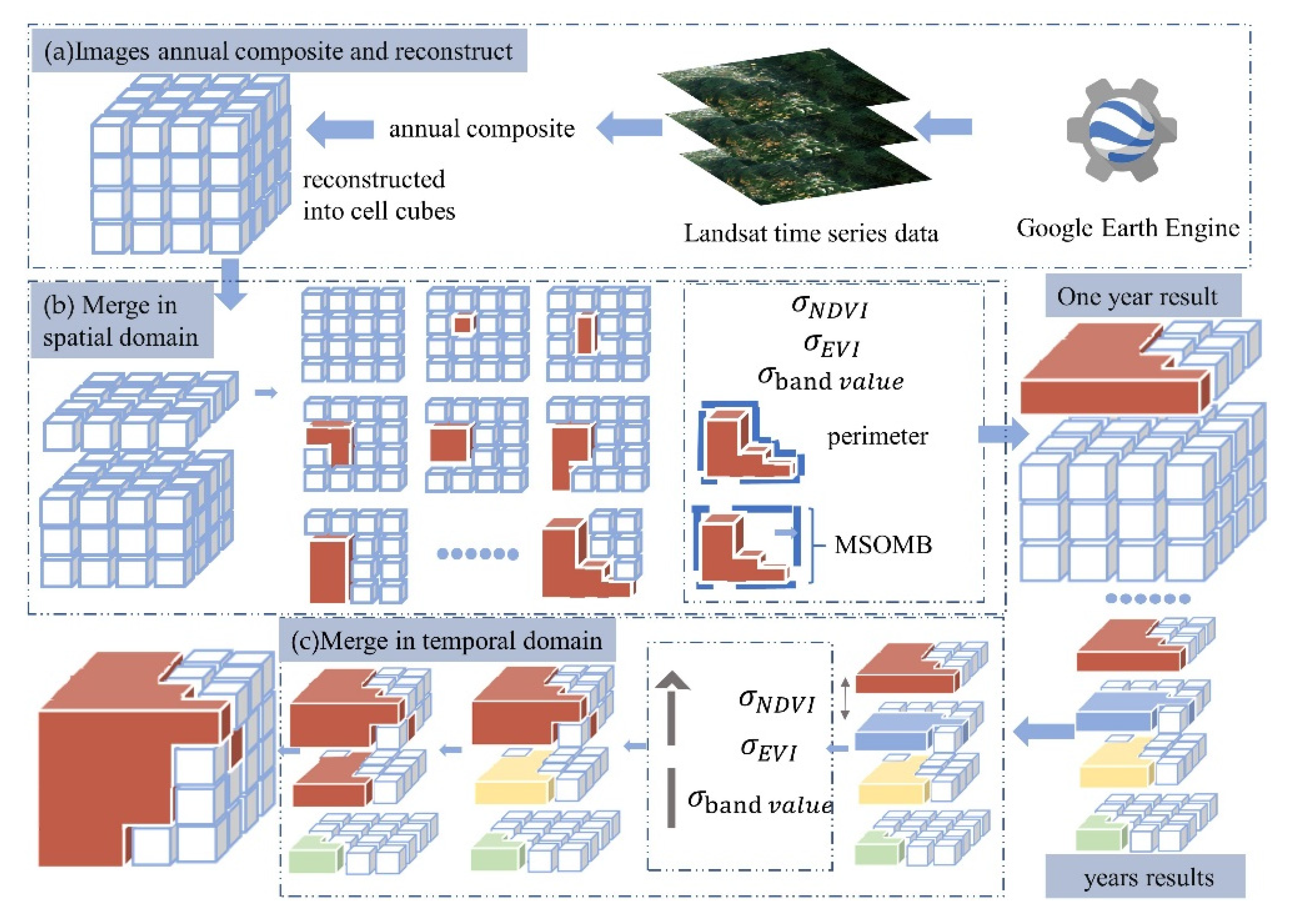
2.2.1. Landsat Time Series and Annual Composite Data

Landsat data are suitable for long time series investigations of forests in the study area because they provide a data record initiated in 1972 with a medium spatial resolution of 30 m [15,41] and six channels ranging from the visual band to the short wave infrared band [42]. Therefore, the Landsat 5 TM, 7 ETM+, and 8 OLI sensors were used as data sources. We used 34 years (1987–2020) of Landsat data (Tier 1, Collection 1), where the effects of atmospheric, topographic, reflectance, and satellite sensors have previously been corrected [43]. All Landsat data were obtained from the Google Earth Engine (GEE) Python API, a cloud computing platform for geospatial analysis [44]. The simpleComposite algorithm on the GEE platform was used to generate annual cloud-free composite scenes of the study area by accessing the median of the least cloudy pixels after converting the images to top-of-atmosphere (TOA) reflectance from all images that fell within each date range [45]. This composite achieved consistency and coherence for forest dynamics monitoring [46,47].

2.2.2. Meteorological Data

Forests are sensitive to meteorological conditions. To account for the fact that the study area is an area with frequent floods and droughts. Therefore, we assume that the major meteorological disasters in the study area are floods and drought. To establish whether the appearance of IST-cubes is related to meteorological disasters, we acquired precipitation data from the Precipitation Estimation from Remotely Sensed Information Using Artificial Neural Networks-Climate Data Record (PERSIANN-CDR), which provided daily global precipitation data from 1983 to the present, with a spatial resolution of 0.25° [48,49]. According to the classification standard of flood and waterlogging weather in Hunan Province, which was developed by the local government [50], a flood is defined as precipitation during any 10 days of more than 200 mm.

Whether drought and IST-cubes appear at the same time is also needs to be compared. Therefore, we introduced Palmer drought severity index (PDSI) as validation data to perform a quantitative evaluation on IST-cubes. PDSI is a widely used drought index to assess the degree of drought [51,52]. PDSI data were acquired from Terra Climate, a global dataset of long-term monthly climate and climatic water balance, with a spatial resolution of 0.04° [53]. The averaged value of all the points of the two data sets in the study area was utilized as the basis for qualitative description of the research area.

2.3. Methodology

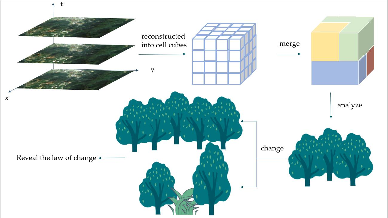
2.3.1. Overview of ST-Cube Model

(1)

Expression and representative significance of ST-cube

In order to correctly describe the spatial-temporal continuity and distribution of geographical objects, Xi [31] proposed the ST-cube model. ST-cubes can reflect the homogeneous state of geographical objects in a certain continuous spatiotemporal range. This feature allows researchers to obtain the spatiotemporal context quantitatively by analyzing the spatiotemporal neighborhood of the ST-cube. As shown in Figure 2a, cube 4 represents an ST-cube with a duration from t0 to t2. During this period, it is homogeneous and has no change. However, cube 1 changes at t1, because it splits into cube 2 and cube 3 at t2.

(2)

Spatiotemporal neighborhoods

The main idea of ST-cube model is to express geographic objects using a cube and realize it by merging pixels or cubes. For a cube, the potential merging objects are the surrounding temporal and spatial neighbors. The definition of a spatial neighbor is that it is adjacent in the spatial domain and intersects in the temporal domain. As shown in Figure 2b, cube 2 and cube 4 are both the spatial neighbors of cube 3 and cube 1. The definition of time neighbor is that it is adjacent in the temporal domain and intersects in the spatial domain. For example, cube 3 is the temporal neighbor of cube 1 and cube 4 is the temporal neighbor of cube 2. After comparing different organizational structures, Xi [31] asserted that the most effective way is as follows: the smallest scale cube is first represented by a pixel, while the large scale cube is generated iteratively by merging small cubes. Therefore, the ST-cube model is an independent pixel at the beginning, which is merged with the spatiotemporal neighbors that meet the merging conditions and have the least heterogeneity to form a large-scale cube. When a pixel merges with its neighbors, they will be regarded as a whole large-scale cube for the next merge judgment.

(3)

Spatiotemporal heterogeneity criterion

Spatiotemporal heterogeneity is used to measure the heterogeneity before and after merger. The judgment basis of spatiotemporal heterogeneity is divided into spatial heterogeneity and temporal heterogeneity. The spatial heterogeneity S_h is defined as a weighted combination of spectral and shape heterogeneity. Temporal heterogeneity T_h is defined as the difference of spectral heterogeneity of spatial cubes before and after merging. Two cubes (cube 1 and cube 2) should be merged into cube0, at least to meet the following requirements:

S_h = ω_shape ·H_shape + (1 − ω_shape)· H_color

(1)

where ${\omega }_{shape}$ is the weight of the shape heterogeneity difference. H_shape and H_color measure the shape difference and spectral difference before and after merging, respectively.

$$T_h=n_{cb}·\Delta T_{cb}·H_t^{cb}-\left(n_{cb1}·\Delta T_{cb1}·H_t^{cb1}+n_{cb2}·\Delta T_{cb2}·H_t^{cb2}\right)$$

(2)

where n is the number of pixels of the bottom of the cube, $\Delta T$ is the length of the ST- cube in the time domain, H_t is the average spectral variance of the ST-cube in the time domain, cb1 and cb2 are the two cubes before merging, and cb is the ST-cube obtained by merging cb1 and cb2. Each ST-cube will find the spatiotemporal neighbor that meets the merging condition and has the least heterogeneity to merge with it until no spatiotemporal neighbor meets the merging condition.

Each ST-cube will find the spatiotemporal neighbor that meets the merging condition and has the least heterogeneity to merge with it until no spatiotemporal neighbor meets the merge condition.

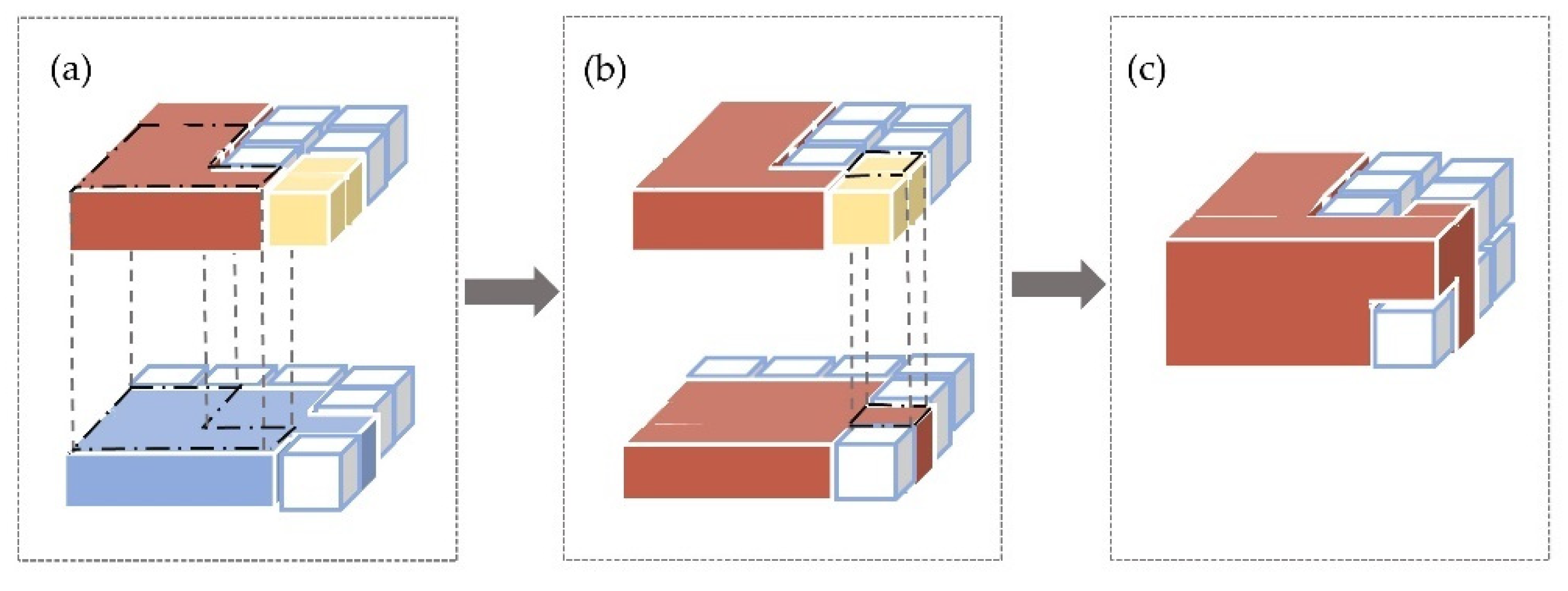
2.3.2. IST-Cube Model

The ST-cube model proposed by Xi [31] has been used and improved in this study. We combined the ST-cube and vegetation indices to develop IST-cube. The essence of this model is to merge IST-cubes or pixels. Before merging, the model successively performs a merger judgment with adjacent IST-cubes, finally merging with the adjacent IST-cube that meets the merger conditions and has the smallest heterogeneity difference.

It has been demonstrated that the NDVI provides important information that can be used to estimate vegetation photosynthesis activity and detect vegetation phenology [54,55]. At the same time, previous studies have established that the EVI can be used to estimate the gross primary production (GPP) [56,57,58]. The EVI has been widely used to monitor the conditions of plants [59,60], which can be calculated using blue and red reflectance bands, as well as near infrared. Both indices have a range between –1 and 1 [61]. Furthermore, previous studies have experimentally demonstrated that using multiple indices yields better performance than the use of a single spectral index [25,62]. Consequently, we chose the parameters and threshold reported in a previous study [31] while adding the EVI and NDVI. Figure 3 presents these details.

A cell cube is the smallest computing unit in the IST-cube model. In this study, a cell cube is defined as a pixel, as in the original model [31], which is determined by the feature that raster data are composed of pixels in a matrix structure. Figure 3a shows that this model reconstructs satellite images into cell cubes before the IST-cube merging. The first step of the IST-cube model (Figure 3b) merges the IST-cube or pixel in the spatial domain every year. This merging method is similar to the region growing method [63]. During this merge, five indicators [i.e., the perimeter of the IST-cube, minimum possible side length of the minimum bounding box (MSOMB) of the IST-cube, standard deviation of the band value, standard deviation of the NDVI, and standard deviation of the EVI] were included in the decision on whether to merge. As shown in Figure 3c, the second step of the IST-cube model merges the IST-cube with adjacent years in the temporal domain. In this study, a two-step procedure (first merge in the spatial domain, followed by merge in the temporal domain) was used for IST-cube merging.

Two IST-cubes must satisfy two conditions to make a merge decision in the temporal domain: 1. they must be adjacent in the temporal domain and 2. they must have at least one pixel with the same X, Y coordinates, as shown in Figure 4, where the red, yellow, and blue IST-cubes represent individual cubes resulting from merging in the spatial domain. Figure 4a shows the red and blue IST-cubes in a time merge judgment because they satisfy two conditions required for a merge decision in the temporal domain. Similarly, Figure 4b displays the result after the red and blue IST-cubes merge into one IST-cube, which is represented by the red IST-cube. The red and yellow IST-cubes then form a time merge judgment. Finally, the yellow and red IST-cubes merge. Figure 4 illustrates that two different IST-cubes can be combined into a single cube by merging with other adjacent IST-cubes in the temporal domain.

Based on a previous study [31], we set the spatial heterogeneity value, S_h, as the sum of the weighted combination of the spectra, shape, EVI, and NDVI:

$$S_h={\omega }_{shape}·H_{shape}+\left(1-{\omega }_{shape}\right)·\left(H_{color}+H_{EVI}+H_{NDVI}\right),$$

(3)

where ${\omega }_{shape}$ ranges between 0 and 1, as decided by the user. In general, ω_shape is a small number that reduces the influence of the shape while spectral has a large weight to scale-up its effect [64]. In this study, the value of 𝜔_shape was set as 0.1 which is a default value [65,66]. The weight of the sum of $H_{color}$, $H_{EVI}$, and $H_{NDVI}$ is determined by 1–${\omega }_{shape}$. Here, $H_{shape}$ determines the shape difference of the IST-cube before and after the merger. In the same manner, $H_{color}$ denotes the spectral difference, as measured by the difference in the standard deviation of all bands before and after merging. $H_{EVI}$ and $H_{NDVI}$ indicate the differences in the vegetation function or greenness, as measured by the difference in the standard deviation of the EVI and NDVI before and after merging.$H_{EVI}$ and $H_{NDVI}$ were calculated as follows:

$$H_{EVI}={\omega }_{EVI}\left[n_{cb}·\Delta T_{cb}·h_{EVI}^{cb}-\left(n_{cb1}·\Delta T_{cb1}·h_{EVI}^{cb1}+n_{cb2}·\Delta T_{cb2}·h_{EVI}^{cb2}\right)\right]\mathrm{and}$$

(4)

$$H_{NDVI}={\omega }_{NDVI}\left[n_{cb}·\Delta T_{cb}·h_{NDVI}^{cb}-\left(n_{cb1}·\Delta T_{cb1}·h_{NDVI}^{cb1}+n_{cb2}·\Delta T_{cb2}·h_{NDVI}^{cb2}\right)\right],$$

(5)

where $h_{EVI}$ and $h_{NDVI}$ are the variance in the EVI and NDVI of the IST-cube, respectively, and ${\omega }_{EVI}$ and ${\omega }_{NDVI}$ are the weights of EVI and NDVI, respectively. For the purpose of forest change detection, this study set ${\omega }_{EVI}$ and ${\omega }_{NDVI}$ as five times the weight of other bands and set ${\omega }_{EVI}$ and ${\omega }_{NDVI}$ as 1.5625 in order to maintain the range of spatiotemporal heterogeneity criterion consistent with the original model. ${\sigma }_{EVI}^i$ and ${\sigma }_{NDVI}^i$ indicate the standard deviation of the EVI and NDVI at time i, respectively, as follows:

$$h_{EVI}=\frac{{{\displaystyle \sum }}_{i=1}^T{\sigma }_{EVI}^i}{T}\mathrm{and}$$

(6)

$$h_{NDVI}=\frac{{{\displaystyle \sum }}_{i=1}^T{\sigma }_{NDVI}^i}{T},$$

(7)

where n is the number of pixels in the spatial domain of the IST-cube at time i, $p_{jEVI}$ and $p_{jNDVI}$ are the EVI and NDVI values of the jth pixel, respectively, and${\overline{p}}_{EVI}$ and ${\overline{p}}_{NDVI}$ are the average EVI and NDVI values of n pixels, respectively. Next, ${\sigma }_{EVI}^i$ and ${\sigma }_{NDVI}^i$ were calculated as follows:

$${\sigma }_{EVI}^i=\sqrt{\frac{{{\displaystyle \sum }}_{jEVI=1}^n{\left(p_{jEVI}-{\overline{p}}_{EVI}\right)}^2}{n}}\mathrm{and}$$

(8)

$${\sigma }_{NDVI}^i=\sqrt{\frac{{{\displaystyle \sum }}_{jNDVI=1}^n{\left(p_{jNDVI}-{\overline{p}}_{NDVI}\right)}^2}{n}},$$

(9)

where $H_t$ refers to the average spectral variance in the IST-cubes in the temporal domain and is normalized as follows:

$$H_t=\frac{{{\displaystyle \sum }}_{i=1}^n\left({{\displaystyle \sum }}_{k=1}^m{\omega }_k·{\sigma }_{tk}^i+{\omega }_{EVI}·{\sigma }_{tEVI}^i+{\omega }_{NDVI}·{\sigma }_{tNDVI}^i\right)}{n},$$

(10)

where m represents the number of bands in the Landsat image, n is the number of pixels at the bottom surface of an IST-cube, and ${\sigma }_{EVI}^i$ and ${\sigma }_{NDVI}^i$ refer to the EVI and NDVI standard deviations in the temporal pixel column formed by pixels of all time point layers in the i-th pixel of the spatial domain, respectively. The normalization of ${\sigma }_{EVI}^i$ and ${\sigma }_{NDVI}^i$ was calculated as follows:

$${\sigma }_{EVI}^i=\sqrt{\frac{{{\displaystyle \sum }}_{j=1}^T{\left(p_{jEVI}-{\overline{p}}_{EVI}\right)}^2}{\Delta T}}\mathrm{and}$$

(11)

$${\sigma }_{NDVI}^i=\sqrt{\frac{{{\displaystyle \sum }}_{j=1}^T{\left(p_{jNDVI}-{\overline{p}}_{NDVI}\right)}^2}{\Delta T}}.$$

(12)

Similarly,${\sigma }_{EVI}^i$ $and {\sigma }_{NDVI}^i$, indicate the EVI and NDVI standard deviations of the temporal pixel column formed by the pixels of all time point layers in the i-th pixel of the spatial domain, respectively.

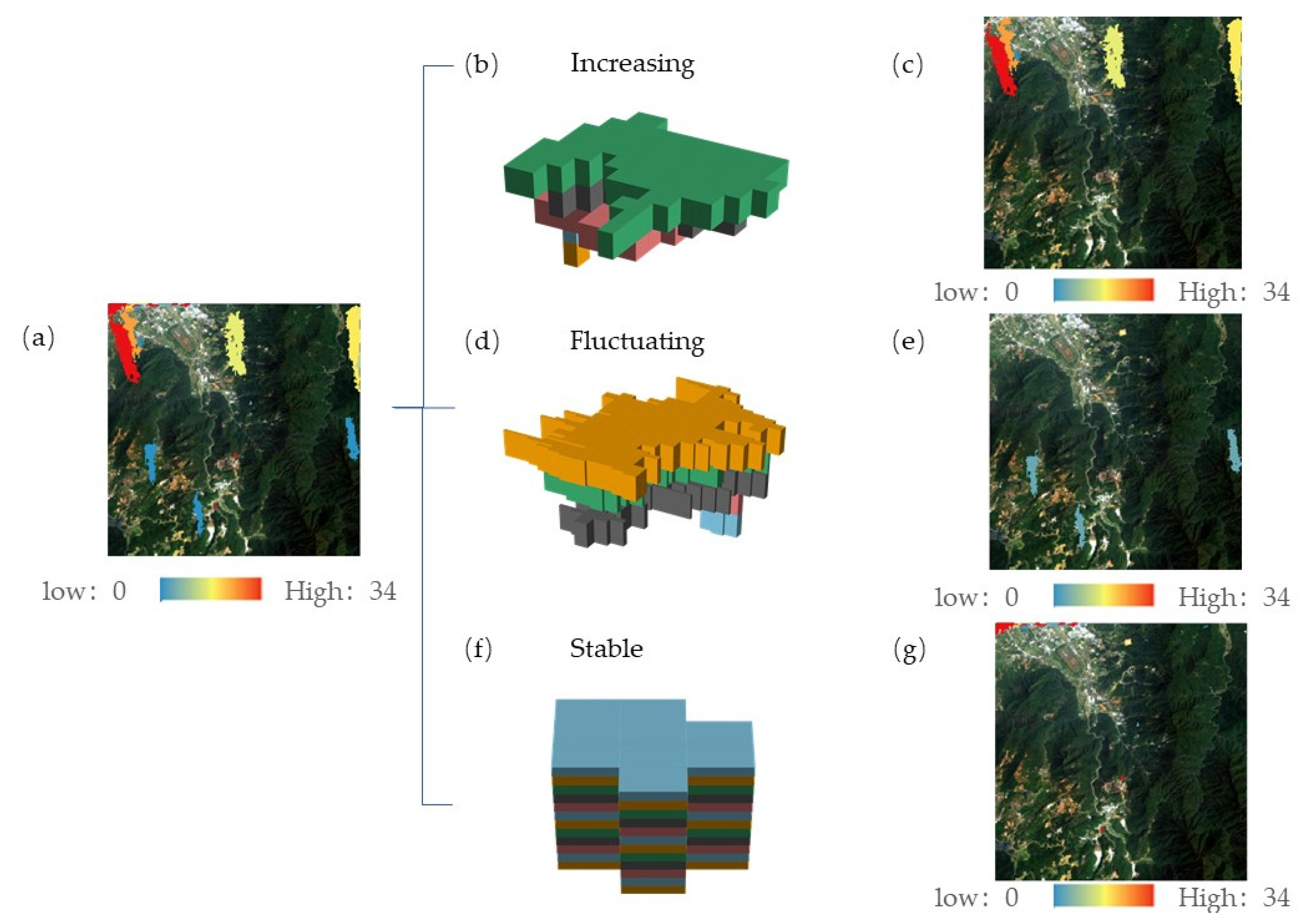
2.3.3. Characteristic Analysis of the IST-Cube

The year when the IST-cube ends is defined as the time when the change occurs; however, numerous IST-cubes fractured suddenly in 2020, as this was the last year of the study period. To avoid this, results were only calculated for 1987–2019. Different changes shape different IST-cubes. Therefore, through the analysis of IST-cubes at different spatiotemporal scales, this study reveals the change law of the study area and explores the corresponding relationship between the change and IST-cubes. The IST-cubes were divided into four types according to the spatiotemporal scale (

Table 1. IST-cube classification and abbreviations based on spatiotemporal scale.

Duration ≥ 5 Years	Average Number of Pixels per Year ≥ 300 Pixels	IST-Cube Type	Abbreviations
Yes	Yes	long-term-large scope	LL
Yes	No	long-term-small scope	LS
No	Yes	short-term-large scope	SL
No	No	short-term-small scope	SS

): long-term-large scope IST-cube, long-term-small scope IST-cube, short-term-large scope IST-cube, and short-term-small scope IST-cube, which were abbreviated as LL, LS, SL, and SS, respectively. This study obtained the trend and slope of the number of pixels per year for the long-term IST-cube (the short-term IST-cube had no trend as their duration was short) using the Mann–Kendall test and Theil-Sen’s slope estimator [67]. This study then further subdivided the long-term IST-cube into four types according to the trends in the number of pixels per year for the long-term IST-cube: monotone increasing, unchanged, alternating increasing and decreasing, and monotone decreasing trends, which are referred to as increasing, stable, fluctuating, and decreasing, respectively. Figure 5 is a schematic diagram of the long-term IST-cube classification process. First, according to the trend obtained by the Mann–Kendall test, it can be divided into the increasing type and the decreasing type. Then, for the IST-cube without trend, it can be further classified according to the slope estimated by Theil-Sen’s slope estimator: if the slope is zero, it is stable type, and if the slope is not zero, it is fluctuating type.

The dynamic time warping (DTW) algorithm is particularly useful in comparing the similarity of unequal time series [68,69,70]. As shown in Figure 6, this study compares the similarity of the time series of the short-term IST-cubes in the same category with the same location but different time points by the DTW. The DTW was calculated by the dtaidistance python module [71]. The smaller the value of DTW, the more similar the two-time series are. To make the DTW value comparable between large scope IST-cube and small scope IST-cube, data were normalized by Z-normalization, which is widely recommended for time series analysis before calculating the DTW [72,73]. However, if there is a large number of situations in that DTW equal to zero, it indicates that there are many similar IST-cubes on the timeline at this location. Further, similar cubes imply the derivation from similar influences, which means a particular change repeatedly affects the IST-cube at this place. Similar changes over and over again mean that the region is changing regularly. In the same way, if DTW is above 0, it means that the region is changing irregularly. Therefore, we referred to these changes that cause these IST-cubes as irregular and regular, respectively.

Different changes resulted in different IST-cubes. Consequently, IST-cubes with diverse spatiotemporal characteristics revealed the regularities of change that shape their structure. This change is unavoidable, and the resulting change for the IST-cube was highly complex and may cause fragmentation of the cube or the merger. The chunk of pixels that was always present in this IST-cube maintained the LL IST-cube structure and acted as a hard core. In this study, we named this the cube-core. A cube-core was defined as a block of pixels inside the LL IST-cube from the beginning to end.

3. Results

According to the IST-cube method, 34 years and 123,827 pixels per year formed 1414 cubes after the calculation. Figure 7 provides an overview of the constituent pixel numbers of the IST-cubes. Most IST-cubes consisted of fewer than 50 pixels. Each cube consisted of an average of 2977 pixels. The smallest cube consisted of only one pixel, whereas the largest cube consisted of 218 283 pixels. Among them, the number of LL IST-cubes, LS IST-cubes, SL IST-cubes, SS IST-cubes are 66, 69,160 and 1119, respectively.

3.1. Long-Term Large Scope IST-Cube

In Figure 8a, the value represents the average duration of the long-term large scope IST-cube in the region, where the higher value is more likely to be dominated by changes that cause this long-term IST-cube. Figure 8a shows that LL IST-cubes exist everywhere in the study area. Figure 8b portrays one cube of the calculated result for the IST-cube model, which contains six layers representing six years, where the number of pixels per year increases, conforming to the LL and increasing IST-cubes. Figure 8d portrays one cube of the calculated result for the IST-cube model, which contains eight layers representing eight years, where the number of pixels per year fluctuates, conforming to the LL and fluctuating IST-cubes. Figure 8a,c show that the principal constituent of LL IST-cubes is the increasing IST-cube, followed by the fluctuating IST-cube. The increasing IST-cube indicates that the spatiotemporal heterogeneity of this cube with its environment is decreasing, whereas a fluctuating change indicates that there is a fluctuation in the spatiotemporal heterogeneity. Figure 8 shows that the LL IST-cube is not characterized by the decreasing and the stable types. However, a specific trigger of the LL could not be determined.

The fluctuating IST-cubes were observed to have no cube-core (Figure 9). The increasing IST-cube core was mainly distributed in residential areas and scattered in the forest. The cube-core located in the forest resembled a disturbance refugia that suffers from severe or frequent disturbances less than the surrounding areas. The cube-core located in the residential area indicated expansion of the area.

3.2. Long-Term Small Scope IST-Cube

As shown in Figure 10a, the value represents the average length of the long-term IST-cube in the region. Figure 10b shows one cube from the calculated results for the IST-cube model, which contains five layers representing five years, where the number of pixels per year is increasing, conforming to the LS and increasing IST-cube classes. Figure 10d is one cube from the calculated results for the IST-cube model, which contains six layers representing six years, where the number of pixels per year is fluctuating, conforming to the LS and fluctuating IST-cube classes. Figure 10d is one cube from the calculated results for the IST-cube model, which contains 13 layers representing 13 years, where the number of pixels per year is stable, thus conforming to the LS and stable IST-cube classes. As shown in Figure 10, the LS IST-cube does not contain the decreasing type.

Figure 10 shows that a significant constituent of the LS IST-cube is the increasing IST-cube, followed by the fluctuating IST-cube and stable IST-cube. In parallel with the increasing and fluctuating IST-cubes, the stable IST-cube indicates spatiotemporal heterogeneity of this cube with its environment with little change. As shown in Figure 10a,g, the stable IST-cube duration is the longest and exists primarily inside residential areas. Residential areas are difficult to change, as their primary component is architecture. Therefore, stable IST-cubes occur inside residential areas. In contrast to the cube-core of the LL IST-cube inside the residential area, but adjacent to the residential area boundary, the LS and stable IST-cube location is closer to the hinterland of the residential area. Accordingly, the hinterland of the residential area, where the LS and stable IST-cubes are located, does not change significantly with time.

Figure 10c shows that the increasing IST-cube is adjacent to residential areas. The residential areas are surrounded by forests and are easily affected by indirect human impacts. An indirect human impact, as defined here, is the impact of daily human life and excludes the vandalism of forests, such as deforestation. The characteristic of the LS and increasing IST-cube classes is long duration, where the spatiotemporal heterogeneity of this cube and its vicinity is decreasing. However, the range of influence is small, which is in accordance with indirect human impacts. Consequently, the LS and increasing IST-cubes classes can be attributed to indirect human impacts.

As shown in Figure 10e, the LS and fluctuating IST-cube classes exist in the mountains, which are located in the western region of the study area, precisely where mining activities are concentrated. A possible explanation for the presence of the LS and fluctuating IST-cube classes may be mining. In summary, this study found that the LS and fluctuating IST-cube classes may be affected by mining. At the same time, the LS and increasing IST-cube classes, occurring around residential areas, are a result of frequent human activity. The LS and stable IST-cube classes exist inside residential areas, which are rarely subject to change.

3.3. Short-Term Large Scope IST-Cube

In contrast to Figure 8 and Figure 10, the index in Figure 11b and Figure 14b denotes the occurrence of short-term IST-cubes. The higher the value, the more frequent the changes that cause such short-term IST-cubes in the study region. Figure 11b shows that the SL IST-cube most often exists in forests, which are located in the eastern region of the study area. Forests are sensitive to meteorological conditions. However, the study area is prone to meteorological disasters. The SL IST-cube is characterized by a short period, but a large influence range, which reflects the characteristics of meteorological disasters. Consequently, SL changes may be explained by meteorological disasters. Figure 12 shows the precipitation and drought from 1987–2019. Figure 12 and

Table 2. Occurrence of floods, droughts, and changes detected by the IST-cube for 1987–2019.

Year	Flood	Drought Class	Is Detected
1987	none	Severe	no
1988	none	Moderate	yes
1989	moderate	Moderate	no
1990	none	Mild	yes
1991	none	Severe	no
1992	moderate	Mild	yes
1993	none	Mild	no
1994	none	None	no
1995	none	None	no
1996	mild	Moderate	yes
1997	mild	Moderate	no
1998	mild	Mild	yes
1999	none	Severe	no
2000	mild	Moderate	no
2001	mild	None	no
2002	none	Mild	no
2003	none	Mild	no
2004	none	Severe	no
2005	none	Severe	no
2006	severe	Moderate	yes
2007	mild	Moderate	no
2008	none	Severe	yes
2009	none	Severe	no
2010	mild	Severe	yes
2011	none	Severe	no
2012	none	Mild	yes
2013	mild	None	no
2014	none	Mild	yes
2015	none	Moderate	no
2016	mild	None	yes
2017	none	Moderate	no
2018	none	Mild	no
2019	mild	Mild	no

indicate that the years in which change was detected were those characterized by floods or droughts.

In contrast to Figure 8 and Figure 10, the index in Figures 11b and 14b denotes the occurrence of short-term IST-cubes. The higher the value, the more frequent the changes that cause such short-term IST-cubes in the study region. Figure 11b shows that the SL IST-cube most often exists in forests, which are located in the eastern region of the study area. Forests are sensitive to meteorological conditions. However, the study area is prone to meteorological disasters. The SL IST-cube is characterized by a short period, but a large influence range, which reflects the characteristics of meteorological disasters. Consequently, SL changes may be explained by meteorological disasters. Figure 12 shows the precipitation and drought from 1987–2019. Figure 12 and Table 2 indicate that the years in which change was detected were those characterized by floods or droughts.

To assess whether the impact of SL IST-cubes that occur in the same region are similar, we used 159 sets of SL IST-cube pixel time series in the DTW computation. The DTW results (Figure 13) indicate that the distance is 0.86 with a standard deviation of 1.13. The 25th, 50th, and 75th percentiles are 0, 0.6, and 0.9, respectively, showing that the SL change is irregular.

3.4. Short-Term Small Scope IST-Cube

Similar to Figure 11b, the index in Figure 14b denotes the occurrence number of short-term IST-cubes. As shown in Figure 14b, the SS IST-cubes are distributed in the residential areas inside, outside, and in one part of the mountain. These areas are high human activity areas characterized by land use changes. The characteristic of the SS IST-cube endures for a short period, where the influence range is small, which is in accordance with the characteristics of land use changes. The SS IST-cubes are likely related to land use change. To validate this hypothesis that the change of land use type leads to the appearance of SS IST-cube, we selected places that exist in the SS IST-cube and visually compared the land use types of the year when the SS IST-cube broke and the following year on Google Earth. Figure 15 shows the comparison results, where the land use in the red box is different before and after the change.

To observe whether the impact of the SS IST-cube that exists in the same region is similar, we used 93 sets of SS IST-cube time series in the DTW computation. The DTW results (Figure 16) exhibited a mean distance of 0.02 and a standard deviation of 0.16, where more than 95.7% of the results were zero, indicating that there are numerous instances of the SS IST-cube, not only in the same place, but also that each impact timing was highly similar. A possible explanation for this may be that most of the changes that caused an SS IST-cube were periodic, e.g., logging.

3.5. Overlap of Different IST-Cube Types

As shown in Figure 17, the study area is primarily composed of different types of IST-cube overlap. Among these, the overlap between the LL IST-cube and LS IST-cube is the most common (82.49% of the study area), followed by the overlap among the LL IST-cube, SL IST-cube, and SS IST-cube (10.44% of the study area). There are three overlap types that were not presented: only the LL IST-cube, only the SS IST-cube, and the overlap between the LS IST-cube and SS IST-cube. Moreover, Figure 16 shows that the changes in the study area are complex.

4. Discussion

We improved the spatiotemporal cube model to provide more detailed spatiotemporal information on forest dynamics and obtained different spatiotemporal scale IST-cubes. Different changes cause different IST-cubes. Consequently, combining the spatial distribution and spatiotemporal features of different IST-cubes can capture the multi-scale spatiotemporal changes in the forests. Our method was tested in a forest rich in mineral resources in China. We mapped the spatial distribution of the IST-cubes at different spatiotemporal scales and analyzed their causes.

4.1. Validation with Literature

The LS IST-cube results support evidence from a previous study that human impact can have long-lasting effects on forests [74,75,76]. Previous studies have shown that meteorological disasters have significant and rapid impacts on forest ecosystems [74,77], which is consistent with the SL IST-cube results. The meteorological disasters shown in Figure 10 and Table 2 have likewise been reported, such as floods in 1998 [78,79,80], drought in 1988 [80], ice disasters in 2008 [81], and other disasters in Chinese meteorological disaster yearbooks [82]. Furthermore, evidence for SS change results was supported by previous studies on forests, which revealed that land use changes have an immediate and partial impact on forests [83,84].

4.2. Advantages of IST-Cube and Other Potential Uses

The IST-cube combines spatiotemporal context information with the forest function index, recognizing and utilizing spatial and temporal changes hidden in spatiotemporal data to analyze regularities and explore causes. Furthermore, the results obtained in this study are consistent with those in the literature (Section 4.1). Figure 10 and Figure 13 and Table 2 show that IST-cube detection is reliable and valid.

Apart from the main aim of developing IST-cube to capture forest dynamics, there are other potential uses. Understanding spatiotemporal changes is important for wetlands [85], which may be fragmented [86]. Nevertheless, the IST-cube can still identify wetland fragments as the same wetland. Thus, the IST-cube may offer a useful method for wetland change detection. Disturbance refugia are locations that suffer severe or frequent disturbances less than their surroundings and can aid in forest recovery from disturbances [9,87]. Fortunately, the cube-core in the long-term IST-cube is such an area that is unaffected by changes. Hence, using the IST-cube model to find disturbance refugia and further analyze the type and duration of disturbance refugia is feasible. Spectral traits will change if plants experience stress, processes, disturbances, and resource limitations [88]. Thus, these traits can also change the appearance of the IST-cube. Therefore, the IST-cube model can also be used to assess vegetation health.

4.3. Limitations and Future Research

Despite these results, questions remain. Table 2 indicates that the SL IST-cube is not characterized by false detections for change years in which meteorological disasters occurred but does contain several missed detections. There is no rule found in these missed detections, and more studies and experiments are needed to explore. Furthermore, we were unable to investigate changes in the vertical structure of the forest, as this study did not include information on these changes. This computationally expensive task results in the small size of the study area, which indicates that capturing large-scale changes in the spatiotemporal domain is not possible. Further studies should attempt to achieve a higher detection accuracy, include more forest structure data, and optimize the algorithm. Long-term earth observation data are limited, and their spatial resolution and temporal resolution depend on sensors. The reason why we chose Landsat as the data source is that Landsat can provide the longest stable earth observation images [89,90]. However, the geographic phenomena observed by a sensor with a determinate spatiotemporal resolution are limited by spatiotemporal scale. Geographic phenomena captured by cell cube are also limited by the spatiotemporal resolution of the sensor. Thus, more studies should focus on using different remote sensing data for the IST-cube model [31].

5. Conclusions

This study aimed to capture and analyze multi-scale spatiotemporal changes. To obtain better results, we improved the ST-cube, renaming it the IST-cube. With the GEE platform, this study used the IST-cube model on the forests of Hunan Province, China, from 1987–2020. Different changes yielded different IST-cubes. Consequently, combining the spatial distribution and spatiotemporal features of different IST-cubes captured the multi-scale spatiotemporal changes. Therefore, this study classified the IST-cube into four spatiotemporal scales according to the spatiotemporal characteristics. For the long-term IST-cube, four types were proposed according to the trends in the number of pixels per year for the long-term IST-cube. The similarity was computed for the short-term IST-cube. The results showed a cube-core that, similar to a hard core, prevented the LL IST-cube from breaking into a short IST-cube. The cube-core in the forest was similar to disturbance refugia. Human activities caused the LS IST-cube, where the impacts surrounding residential areas were increasing with no interior changes. Meteorological disasters led to the SL IST-cube, where the impact of meteorological disasters was irregular. The changes in land use or logging, as well as fires, caused SS IST-cubes and similar impacts. The results of this study provide enhanced insights into forest changes. The IST-cube model we improved in this paper is a novel and useful model for forest change detection.

References

1. Fujii, S.; Mori, A.S.; Koide, D.; Makoto, K.; Matsuoka, S.; Osono, T.; Isbell, F. Disentangling relationships between plant diversity and decomposition processes under forest restoration. J. Appl. Ecol. 2017, 54, 80–90. [Google Scholar] [CrossRef]
2. Curtis, P.G.; Slay, C.M.; Harris, N.L.; Tyukavina, A.; Hansen, M.C. Classifying drivers of global forest loss. Science 2018, 361, 1108–1111. [Google Scholar] [CrossRef] [PubMed]
3. Sturrock, R.; Frankel, S.; Brown, A.; Hennon, P.; Kliejunas, J.; Lewis, K.; Worrall, J.; Woods, A. Climate change and forest diseases. Plant Pathol. 2011, 60, 133–149. [Google Scholar] [CrossRef]
4. Watson, J.E.; Evans, T.; Venter, O.; Williams, B.; Tulloch, A.; Stewart, C.; Thompson, I.; Ray, J.C.; Murray, K.; Salazar, A. The exceptional value of intact forest ecosystems. Nat. Ecol. Evol. 2018, 2, 599–610. [Google Scholar] [CrossRef]
5. Overpeck, J.T.; Rind, D.; Goldberg, R. Climate-induced changes in forest disturbance and vegetation. Nature 1990, 343, 51–53. [Google Scholar] [CrossRef]
6. Maynard, D.; Paré, D.; Thiffault, E.; Lafleur, B.; Hogg, K.; Kishchuk, B. How do natural disturbances and human activities affect soils and tree nutrition and growth in the Canadian boreal forest? Environ. Rev. 2014, 22, 161–178. [Google Scholar] [CrossRef]
7. Lal, R. Forest soils and carbon sequestration. For. Ecol. Manag. 2005, 220, 242–258. [Google Scholar] [CrossRef]
8. Wei, C.; Karger, D.N.; Wilson, A.M. Spatial detection of alpine treeline ecotones in the Western United States. Remote Sens. Environ. 2020, 240. [Google Scholar] [CrossRef]
9. Krawchuk, M.A.; Meigs, G.W.; Cartwright, J.M.; Coop, J.D.; Davis, R.; Holz, A.; Kolden, C.; Meddens, A.J. Disturbance refugia within mosaics of forest fire, drought, and insect outbreaks. Front. Ecol. Environ. 2020, 18, 235–244. [Google Scholar] [CrossRef]
10. Eshleman, K.N.; McNeil, B.E.; Townsend, P.A. Validation of a remote sensing based index of forest disturbance using streamwater nitrogen data. Ecol. Indic. 2009, 9, 476–484. [Google Scholar] [CrossRef]
11. McDowell, N.G.; Coops, N.C.; Beck, P.S.; Chambers, J.Q.; Gangodagamage, C.; Hicke, J.A.; Huang, C.-y.; Kennedy, R.; Krofcheck, D.J.; Litvak, M. Global satellite monitoring of climate-induced vegetation disturbances. Trends Plant Sci. 2015, 20, 114–123. [Google Scholar] [CrossRef] [PubMed] [Green Version]
12. Wulder, M.A.; Kurz, W.A.; Gillis, M. National level forest monitoring and modeling in Canada. Prog. Plan. 2004, 61, 365–381. [Google Scholar] [CrossRef]
13. Hermosilla, T.; Wulder, M.A.; White, J.C.; Coops, N.C. Prevalence of multiple forest disturbances and impact on vegetation regrowth from interannual Landsat time series (1985–2015). Remote Sens. Environ. 2019, 233, 111403. [Google Scholar] [CrossRef]
14. Banskota, A.; Kayastha, N.; Falkowski, M.J.; Wulder, M.A.; Froese, R.E.; White, J.C. Forest monitoring using Landsat time series data: A review. Can. J. Remote Sens. 2014, 40, 362–384. [Google Scholar] [CrossRef]
15. Shimizu, K.; Ota, T.; Mizoue, N. Detecting forest changes using dense Landsat 8 and Sentinel-1 time series data in tropical seasonal forests. Remote Sens. 2019, 11, 1899. [Google Scholar] [CrossRef] [Green Version]
16. Kayet, N.; Pathak, K.; Chakrabarty, A.; Singh, C.P.; Sahoo, S. Forest health assessment for geo-environmental planning and management in hilltop mining areas using Hyperion and Landsat data. Ecol. Indic. 2019, 106, 105471. [Google Scholar] [CrossRef]
17. Chen, X.-L.; Zhao, H.-M.; Li, P.-X.; Yin, Z.-Y. Remote sensing image-based analysis of the relationship between urban heat island and land use/cover changes. Remote Sens. Environ. 2006, 104, 133–146. [Google Scholar] [CrossRef]
18. Hossain, M.D.; Chen, D. Segmentation for object-based image analysis (obia): A review of algorithms and challenges from remote sensing perspective. ISPRS J. Photogramm. Remote Sens. 2019, 150, 115–134. [Google Scholar] [CrossRef]
19. Xu, J.; Zhao, H.; Yin, P.; Jia, D.; Li, G. Remote sensing classification method of vegetation dynamics based on time series Landsat image: A case of opencast mining area in China. EURASIP J. Image Video Process. 2018, 2018, 1–10. [Google Scholar] [CrossRef]
20. Caballero Espejo, J.; Messinger, M.; Román-Dañobeytia, F.; Ascorra, C.; Fernandez, L.E.; Silman, M. Deforestation and forest degradation due to gold mining in the Peruvian Amazon: A 34-year perspective. Remote Sens. 2018, 10, 1903. [Google Scholar] [CrossRef] [Green Version]
21. Souza-Filho, P.W.M.; Nascimento, W.R.; Santos, D.C.; Weber, E.J.; Silva, R.O.; Siqueira, J.O. A GEOBIA approach for multitemporal land-cover and land-use change analysis in a tropical watershed in the southeastern Amazon. Remote Sens. 2018, 10, 1683. [Google Scholar] [CrossRef] [Green Version]
22. Hermosilla, T.; Wulder, M.A.; White, J.C.; Coops, N.C.; Hobart, G.W. Regional detection, characterization, and attribution of annual forest change from 1984 to 2012 using Landsat-derived time-series metrics. Remote Sens. Environ. 2015, 170, 121–132. [Google Scholar] [CrossRef]
23. Yang, Z.; Li, J.; Zipper, C.E.; Shen, Y.; Miao, H.; Donovan, P.F. Identification of the disturbance and trajectory types in mining areas using multitemporal remote sensing images. Sci. Total Environ. 2018, 644, 916–927. [Google Scholar] [CrossRef]
24. Meng, Y.; Liu, X.; Ding, C.; Xu, B.; Zhou, G.; Zhu, L. Analysis of ecological resilience to evaluate the inherent maintenance capacity of a forest ecosystem using a dense Landsat time series. Ecol. Inform. 2020, 57. [Google Scholar] [CrossRef]
25. Cohen, W.B.; Yang, Z.; Healey, S.P.; Kennedy, R.E.; Gorelick, N. A LandTrendr multispectral ensemble for forest disturbance detection. Remote Sens. Environ. 2018, 205, 131–140. [Google Scholar] [CrossRef]
26. Cohen, W.B.; Healey, S.P.; Yang, Z.; Stehman, S.V.; Brewer, C.K.; Brooks, E.B.; Gorelick, N.; Huang, C.; Hughes, M.J.; Kennedy, R.E. How similar are forest disturbance maps derived from different Landsat time series algorithms? Forests 2017, 8, 98. [Google Scholar] [CrossRef]
27. Vogelmann, J.E.; Tolk, B.; Zhu, Z. Monitoring forest changes in the southwestern United States using multitemporal Landsat data. Remote Sens. Environ. 2009, 113, 1739–1748. [Google Scholar] [CrossRef]
28. Kennedy, R.E.; Yang, Z.; Cohen, W.B. Detecting trends in forest disturbance and recovery using yearly Landsat time series: 1. LandTrendr—Temporal segmentation algorithms. Remote Sens. Environ. 2010, 114, 2897–2910. [Google Scholar] [CrossRef]
29. Kang, Y.; Cho, N.; Son, S. Spatiotemporal characteristics of elderly population’s traffic accidents in Seoul using space-time cube and space-time kernel density estimation. PLoS ONE 2018, 13, e0196845. [Google Scholar] [CrossRef] [PubMed] [Green Version]
30. Mo, C.; Tan, D.; Mai, T.; Bei, C.; Qin, J.; Pang, W.; Zhang, Z. An analysis of spatiotemporal pattern for COIVD-19 in China based on space-time cube. J. Med. Virol. 2020, 92, 1587–1595. [Google Scholar] [CrossRef] [PubMed] [Green Version]
31. Xi, W.; Du, S.; Wang, Y.-C.; Zhang, X. A spatiotemporal cube model for analyzing satellite image time series: Application to land-cover mapping and change detection. Remote Sens. Environ. 2019, 231, 111212. [Google Scholar] [CrossRef]
32. Trumbore, S.; Brando, P.; Hartmann, H. Forest health and global change. Science 2015, 349, 814–818. [Google Scholar] [CrossRef] [Green Version]
33. Upadhyay, T.; Sankhayan, P.L.; Solberg, B. A review of carbon sequestration dynamics in the Himalayan region as a function of land-use change and forest/soil degradation with special reference to Nepal. Agric. Ecosyst. Environ. 2005, 105, 449–465. [Google Scholar] [CrossRef]
34. Chu, H.; Venevsky, S.; Wu, C.; Wang, M. NDVI-based vegetation dynamics and its response to climate changes at Amur-Heilongjiang River Basin from 1982 to 2015. Sci. Total Environ. 2019, 650, 2051–2062. [Google Scholar] [CrossRef] [PubMed]
35. Lamchin, M.; Lee, W.-K.; Jeon, S.W.; Wang, S.W.; Lim, C.H.; Song, C.; Sung, M. Long-term trend and correlation between vegetation greenness and climate variables in Asia based on satellite data. Sci. Total Environ. 2018, 618, 1089–1095. [Google Scholar] [CrossRef]
36. Tucker, C.J.; Holben, B.N.; Goff, T.E. Intensive forest clearing in Rondonia, Brazil, as detected by satellite remote sensing. Remote Sens. Environ. 1984, 15, 255–261. [Google Scholar] [CrossRef]
37. Zhu, Z.; Fu, Y.; Woodcock, C.E.; Olofsson, P.; Vogelmann, J.E.; Holden, C.; Wang, M.; Dai, S.; Yu, Y. Including land cover change in analysis of greenness trends using all available Landsat 5, 7, and 8 images: A case study from Guangzhou, China (2000–2014). Remote Sens. Environ. 2016, 185, 243–257. [Google Scholar] [CrossRef] [Green Version]
38. Yang, Q.; Zhang, H.; Peng, W.; Lan, Y.; Luo, S.; Shao, J.; Chen, D.; Wang, G. Assessing climate impact on forest cover in areas undergoing substantial land cover change using Landsat imagery. Sci. Total Environ. 2019, 659, 732–745. [Google Scholar] [CrossRef]
39. Gurung, R.B.; Breidt, F.J.; Dutin, A.; Ogle, S.M. Predicting Enhanced Vegetation Index (EVI) curves for ecosystem modeling applications. Remote Sens. Environ. 2009, 113, 2186–2193. [Google Scholar] [CrossRef]
40. Cheng, Y.; Wang, Y.; Tan, R. Trace Element Geochemistry of Devonian Strata in the Shizhuyuan Ore District, Hunan Province. Acta Geol. Sin. 2017, 1, 175–176. [Google Scholar] [CrossRef] [Green Version]
41. Frazier, R.J.; Coops, N.C.; Wulder, M.A.; Hermosilla, T.; White, J.C. Analyzing spatial and temporal variability in short-term rates of post-fire vegetation return from Landsat time series. Remote Sens. Environ. 2018, 205, 32–45. [Google Scholar] [CrossRef]
42. Zhu, C.; Zhang, X.; Zhang, N.; Hassan, M.A.; Zhao, L. Assessing the defoliation of pine forests in a long time-series and spatiotemporal prediction of the defoliation using Landsat data. Remote Sens. 2018, 10, 360. [Google Scholar] [CrossRef] [Green Version]
43. Xie, Z.; Phinn, S.R.; Game, E.T.; Pannell, D.J.; Hobbs, R.J.; Briggs, P.R.; McDonald-Madden, E. Using Landsat observations (1988–2017) and Google Earth Engine to detect vegetation cover changes in rangelands-A first step towards identifying degraded lands for conservation. Remote Sens. Environ. 2019, 232, 111317. [Google Scholar] [CrossRef]
44. Gorelick, N.; Hancher, M.; Dixon, M.; Ilyushchenko, S.; Thau, D.; Moore, R. Google Earth Engine: Planetary-scale geospatial analysis for everyone. Remote Sens. Environ. 2017, 202, 18–27. [Google Scholar] [CrossRef]
45. Ward, E.M.; Gorelick, S.M. Drying drives decline in muskrat population in the Peace-Athabasca Delta, Canada. Environ. Res. Lett. 2018, 13, 124026. [Google Scholar] [CrossRef]
46. Roberts, L.J.; Burnett, R.; Tietz, J.; Veloz, S. Recent drought and tree mortality effects on the avian community in southern Sierra Nevada: A glimpse of the future? Ecol. Appl. 2019, 29, e01848. [Google Scholar] [CrossRef]
47. Huang, J.; McBratney, A.B.; Malone, B.P.; Field, D.J. Mapping the transition from pre-European settlement to contemporary soil conditions in the Lower Hunter Valley, Australia. Geoderma 2018, 329, 27–42. [Google Scholar] [CrossRef]
48. Sorooshian, S.; Hsu, K.; Braithwaite, D.; Ashouri, H. The NOAA CDR Program, 2014: NOAA Climate Data Record (CDR) of Precipitation Estimation from Remotely Sensed Information using Artificial Neural Networks (PERSIANN-CDR), version 1, revision 1. NOAA Natl. Cent. Environ. Inf. Accessed 2015, 18. [Google Scholar] [CrossRef]
49. Ashouri, H.; Hsu, K.L.; Sorooshian, S.; Braithwaite, D.K.; Knapp, K.R.; Cecil, L.D.; Nelson, B.R.; Prat, O.P. PERSIANNCDR: Daily precipitation climate data record from multisatellite observations for hydrological and climate studies. Bull. Am. Meteor. Soc. 2015, 96, 69–83. [Google Scholar] [CrossRef] [Green Version]
50. Hunan Meteorological Bureau. Classification standard of flood and waterlogging weather in Hunan Province. Available online: http://hn.cma.gov.cn/xxgk/gkml/tzgg/202012/t20201202_2449482.html (accessed on 7 January 2021).
51. Palmer, W.C. Meteorological Drought; US Department of Commerce, Weather Bureau: Washington, DC, USA, 1965; Volume 30. [Google Scholar]
52. Yan, H.; Wang, S.Q.; Wang, J.B.; Lu, H.Q.; Guo, A.H.; Zhu, Z.C.; Myneni, R.B.; Shugart, H.H. Assessing spatiotemporal variation of drought in China and its impact on agriculture during 1982–2011 by using PDSI indices and agriculture drought survey data. J. Geophys. Res. Atmos. 2016, 121, 2283–2298. [Google Scholar] [CrossRef] [Green Version]
53. Abatzoglou, J.T.; Dobrowski, S.Z.; Parks, S.A.; Hegewisch, K.C. TerraClimate, a high-resolution global dataset of monthly climate and climatic water balance from 1958–2015. Sci. Data 2018, 5, 1–12. [Google Scholar] [CrossRef] [Green Version]
54. Zhang, X.; Tarpley, D.; Sullivan, J.T. Diverse responses of vegetation phenology to a warming climate. Geophys. Res. Lett. 2007, 34. [Google Scholar] [CrossRef]
55. Cao, R.; Chen, Y.; Shen, M.; Chen, J.; Zhou, J.; Wang, C.; Yang, W. A simple method to improve the quality of NDVI time-series data by integrating spatiotemporal information with the Savitzky-Golay filter. Remote Sens. Environ. 2018, 217, 244–257. [Google Scholar] [CrossRef]
56. Hinojo-Hinojo, C.; Goulden, M.L. Plant Traits Help Explain the Tight Relationship between Vegetation Indices and Gross Primary Production. Remote Sens. 2020, 12, 1405. [Google Scholar] [CrossRef]
57. Sims, D.A.; Rahman, A.F.; Cordova, V.D.; El-Masri, B.Z.; Baldocchi, D.D.; Flanagan, L.B.; Goldstein, A.H.; Hollinger, D.Y.; Misson, L.; Monson, R.K.; et al. On the use of MODIS EVI to assess gross primary productivity of North American ecosystems. J. Geophys. Res. Biogeosci. 2006, 111. [Google Scholar] [CrossRef] [Green Version]
58. Hashimoto, H.; Wang, W.; Milesi, C.; White, M.A.; Ganguly, S.; Gamo, M.; Hirata, R.; Myneni, R.B.; Nemani, R.R. Exploring Simple Algorithms for Estimating Gross Primary Production in Forested Areas from Satellite Data. Remote Sens. 2012, 4, 303–326. [Google Scholar] [CrossRef] [Green Version]
59. Son, N.; Chen, C.; Chen, C.; Minh, V.; Trung, N. A comparative analysis of multitemporal MODIS EVI and NDVI data for large-scale rice yield estimation. Agric. For. Meteorol. 2014, 197, 52–64. [Google Scholar] [CrossRef]
60. Chen, H.; Liang, Q.; Liang, Z.; Liu, Y.; Xie, S. Remote-sensing disturbance detection index to identify spatio-temporal varying flood impact on crop production. Agric. For. Meteorol. 2019, 269–270, 180–191. [Google Scholar] [CrossRef]
61. Huete, A.; Didan, K.; Miura, T.; Rodriguez, E.P.; Gao, X.; Ferreira, L.G. Overview of the radiometric and biophysical performance of the MODIS vegetation indices. Remote Sens. Environ. 2002, 83, 195–213. [Google Scholar] [CrossRef]
62. Zhu, Z.; Zhang, J.; Yang, Z.; Aljaddani, A.H.; Cohen, W.B.; Qiu, S.; Zhou, C. Continuous monitoring of land disturbance based on Landsat time series. Remote Sens. Environ. 2020, 238. [Google Scholar] [CrossRef]
63. Adams, R.; Bischof, L. Seeded region growing. IEEE Trans. Pattern Anal. Mach. Intell. 1994, 16, 641–647. [Google Scholar] [CrossRef] [Green Version]
64. Ming, D.; Zhou, W.; Xu, L.; Wang, M.; Ma, Y. Coupling relationship among scale parameter, segmentation accuracy, and classification accuracy in geobia. Photogramm. Eng. Remote Sens. 2018, 84, 681–693. [Google Scholar] [CrossRef]
65. Baatz, M. Multi resolution segmentation: An optimum approach for high quality multi scale image segmentation. In Beutrage zum AGIT-Symposium; Salzburg: Heidelberg, Germany, 2000; pp. 12–23. [Google Scholar]
66. Drăguţ, L.; Csillik, O.; Eisank, C.; Tiede, D. Automated parameterisation for multi-scale image segmentation on multiple layers. ISPRS J. Photogramm. Remote Sens. 2014, 88, 119–127. [Google Scholar] [CrossRef] [Green Version]
67. Hussain, M.M.; Mahmud, I. pyMannKendall: A python package for non parametric Mann Kendall family of trend tests. J. Open Source Softw. 2019, 4, 1556. [Google Scholar] [CrossRef]
68. Bellman, R.; Kalaba, R. On adaptive control processes. IRE Trans. Autom. Control 1959, 4, 1–9. [Google Scholar] [CrossRef]
69. Petitjean, F.; Inglada, J.; Gançarski, P. Satellite image time series analysis under time warping. IEEE Trans. Geosci. Remote Sens. 2012, 50, 3081–3095. [Google Scholar] [CrossRef]
70. Guan, X.; Huang, C.; Liu, G.; Meng, X.; Liu, Q. Mapping rice cropping systems in Vietnam using an NDVI-based time-series similarity measurement based on DTW distance. Remote Sens. 2016, 8, 19. [Google Scholar] [CrossRef] [Green Version]
71. Wannes Meert, K.H. Toon Van Craenendonck. (Version v2.0.0). Available online: https://github.com/wannesm/dtaidistance (accessed on 8 January 2021).
72. Mueen, A.; Keogh, E. Extracting optimal performance from dynamic time warping. In Proceedings of the 22nd ACM SIGKDD International Conference on Knowledge Discovery and Data Mining, San Francisco, CA, USA, 13–17 August 2016; pp. 2129–2130. [Google Scholar]
73. Liu, H.; Zhan, Q.; Yang, C.; Wang, J. Characterizing the spatio-temporal pattern of land surface temperature through time series clustering: Based on the latent pattern and morphology. Remote Sens. 2018, 10, 654. [Google Scholar] [CrossRef] [Green Version]
74. Chazdon, R.L. Tropical forest recovery: Legacies of human impact and natural disturbances. Perspect. Plant Ecol. Evol. Syst. 2003, 6, 51–71. [Google Scholar] [CrossRef] [Green Version]
75. Canadell, J.G.; Kirschbaum, M.U.; Kurz, W.A.; Sanz, M.-J.; Schlamadinger, B.; Yamagata, Y. Factoring out natural and indirect human effects on terrestrial carbon sources and sinks. Environ. Sci. Policy 2007, 10, 370–384. [Google Scholar] [CrossRef]
76. Vetter, M.; Wirth, C.; Böttcher, H.; Churkina, G.; Schulze, E.D.; Wutzler, T.; Weber, G. Partitioning direct and indirect human-induced effects on carbon sequestration of managed coniferous forests using model simulations and forest inventories. Glob. Chang. Biol. 2005, 11, 810–827. [Google Scholar] [CrossRef]
77. Bhattacharjee, K.; Behera, B. Forest cover change and flood hazards in India. Land Use Policy 2017, 67, 436–448. [Google Scholar] [CrossRef]
78. Liu, A.; Tan, H.; Zhou, J.; Li, S.; Yang, T.; Wang, J.; Liu, J.; Tang, X.; Sun, Z.; Wen, S.W. An epidemiologic study of posttraumatic stress disorder in flood victims in Hunan China. Can. J. Psychiat. 2006, 51, 350–354. [Google Scholar] [CrossRef] [Green Version]
79. Huang, X.; Tan, H.; Zhou, J.; Yang, T.; Benjamin, A.; Wen, S.W.; Li, S.; Liu, A.; Li, X.; Fen, S. Flood hazard in Hunan province of China: An economic loss analysis. Nat. Hazard. 2008, 47, 65–73. [Google Scholar] [CrossRef]
80. Du, J.; Fang, J.; Xu, W.; Shi, P. Analysis of dry/wet conditions using the standardized precipitation index and its potential usefulness for drought/flood monitoring in Hunan Province, China. Stoch. Environ. Res. Risk Assess. 2013, 27, 377–387. [Google Scholar] [CrossRef]
81. Wu, D.; Yin, H.; Xu, S.; Zhao, Y. Risk factors for posttraumatic stress reactions among Chinese students following exposure to a snowstorm disaster. BMC Public Health 2011, 11, 96. [Google Scholar] [CrossRef] [Green Version]
82. Song, L.; Fan, Y. Yearbook of Meterorological Disasters in China; China Meteorological Press: Beijing, China, 2012. [Google Scholar]
83. Abdullah, S.A.; Nakagoshi, N. Forest fragmentation and its correlation to human land use change in the state of Selangor, peninsular Malaysia. For. Ecol. Manag. 2007, 241, 39–48. [Google Scholar] [CrossRef]
84. Viedma, O.; Moreno, J.M.; Rieiro, I. Interactions between land use/land cover change, forest fires and landscape structure in Sierra de Gredos (Central Spain). Environ. Conserv. 2006, 33, 212–222. [Google Scholar] [CrossRef]
85. Guo, M.; Li, J.; Sheng, C.; Xu, J.; Wu, L. A review of wetland remote sensing. Sensors 2017, 17, 777. [Google Scholar] [CrossRef] [Green Version]
86. Lu, C.; Ren, C.; Wang, Z.; Zhang, B.; Man, W.; Yu, H.; Gao, Y.; Liu, M. Monitoring and Assessment of Wetland Loss and Fragmentation in the Cross-Boundary Protected Area: A Case Study of Wusuli River Basin. Remote Sens. 2019, 11, 2581. [Google Scholar] [CrossRef] [Green Version]
87. Keppel, G.; Van Niel, K.P.; Wardell-Johnson, G.W.; Yates, C.J.; Byrne, M.; Mucina, L.; Schut, A.G.T.; Hopper, S.D.; Franklin, S.E. Refugia: Identifying and understanding safe havens for biodiversity under climate change. Glob. Ecol. Biogeogr. 2012, 21, 393–404. [Google Scholar] [CrossRef]
88. Lausch, A.; Bastian, O.; Klotz, S.; Leitão, P.J.; Jung, A.; Rocchini, D.; Schaepman, M.E.; Skidmore, A.K.; Tischendorf, L.; Knapp, S. Understanding and assessing vegetation health by in situ species and remote-sensing approaches. Methods Ecol. Evol. 2018, 9, 1799–1809. [Google Scholar] [CrossRef]
89. Ye, S.; Rogan, J.; Zhu, Z.; Eastman, J.R. A near-real-time approach for monitoring forest disturbance using Landsat time series: Stochastic continuous change detection. Remote Sens. Environ. 2021, 252, 112167. [Google Scholar] [CrossRef]
90. Masek, J.G.; Goward, S.N.; Kennedy, R.E.; Cohen, W.B.; Moisen, G.G.; Schleeweis, K.; Huang, C. United States forest disturbance trends observed using Landsat time series. Ecosystems 2013, 16, 1087–1104. [Google Scholar] [CrossRef] [Green Version]
Figure 1. Location of the study area in Hunan Province, China.
Remotesensing 13 02537 g001
Figure 2. (a) Expression of ST-cube. The X and Y axes represent the spatial domain, and the T-axis represents the temporal domain. (b) Schematic diagram of spatiotemporal neighborhoods.
Remotesensing 13 02537 g002
Figure 3. Methodological flowchart for the (a) annual composite and reconstruct and (b) merging the IST-cube in the spatial domain. MSOMB = minimum possible side length of the minimum bounding box. (c) Merging the IST-cube in the temporal domain.
Remotesensing 13 02537 g003
Figure 4. Schematic merging of the spatial results for the IST-cube in the temporal domain. Red, yellow, and blue cubes represent individual cubes resulting from merging in the spatial domain. (a) Red and blue IST-cubes in the merge judgment in the temporal domain; (b) red and yellow IST-cubes in the merge judgment in the temporal domain; and (c) final merge into a single cube.
Remotesensing 13 02537 g004
Figure 5. Flow diagram of the long-term IST-cube classification. The cube in the figure has different colors for different years. The cubes that appear in the following figures are all the same.
Remotesensing 13 02537 g005
Figure 6. Schematic diagram of DTW calculation method for short-term IST-cube.
Remotesensing 13 02537 g006
Figure 7. IST-cube containing the number of pixels distribution. (a) General sketch of the IST-cube containing the number of pixels distribution. (b) Line chart of the distribution of the IST-cube, whose constituent pixels are less than 50. (c) Box plot of the IST-cube distribution, where the constituent pixels are more than 50.
Remotesensing 13 02537 g007
Figure 8. (a) Spatial distribution of the mean time length of the LL IST-cube. (b) Actual LL and increasing IST-cube diagram, containing six layers representing a six-year duration, with an increasing number of pixels per year, conforming to the LL and increasing IST-cube classes. (c) Spatial distribution of the mean time length for the LL and increasing IST-cube classes. (d) Actual LL and fluctuating IST-cube diagram, containing eight layers representing an eight-year duration, with a fluctuating number of pixels per year, conforming to the LL and fluctuating IST-cube classes. (e) Spatial distribution of the mean time length for the LL and fluctuating IST-cube classes.
Remotesensing 13 02537 g008
Figure 9. Spatial distribution map of LL IST-cube cube-core.
Remotesensing 13 02537 g009
Figure 10. (a) Spatial distribution map of the mean time length of the LS IST-cube. (b) Actual LS and increasing IST-cube diagram, containing five layers representing five years, with an increasing number of pixels per year, conforming to the LS and increasing IST-cube classes. (c) Spatial distribution map of the mean time length of the LS and increasing IST-cube classes. (d) Actual LS and fluctuating IST-cube diagram, containing six layers representing six years, with a fluctuating number of pixels per year, conforming to the LS and fluctuating IST-cube classes. (e) Spatial distribution map of the mean time length of the LS and fluctuating IST-cube classes. (f) Actual LS and stable IST-cube diagram, containing 13 layers representing 13 years, where the number of pixels per year is constant, conforming to the LS and stable IST-cube classes. (g) Spatial distribution map of the mean time length of the LS and stable IST-cube classes.
Remotesensing 13 02537 g010
Figure 11. (a) Actual SL IST-cube diagram containing two layers representing two years. The average number of pixels per year is 14 647, conforming to the criterion for the SL IST-cube class. (b) Spatial distribution map of occurrence number for the SL IST-cube.
Remotesensing 13 02537 g011
Figure 12. Precipitation and drought for 1987–2019. (a) Maximum precipitation and flood threshold for 10 consecutive days and (b) proportion of drought periods.
Remotesensing 13 02537 g012
Figure 13. Distance of SL change calculated using DTW. (a) Line chart of the DTW result distribution. (b) Cumulative percentage of the DTW result.
Remotesensing 13 02537 g013
Figure 14. (a) Actual SS IST-cube diagram, containing three layers representing three years. The average number of pixels per year is 13, conforming to the criterion for the SS IST-cube class. (b) Spatial distribution map of occurrence number of the SS IST-cube.
Remotesensing 13 02537 g014
Figure 15. Assessment examples of SS change. (a) SS change in the study area (Figure 14b) with two marked examples of change. Images from Landsat and Google Earth show the changes before and after in the forests. (b) Land use change in 2001 and (c) land use change in 2019.
Remotesensing 13 02537 g015
Figure 16. Distance for the SS change calculated using DTW. (a) Line chart of the DTW result distribution. (b) Cumulative percentage of the DTW result.
Remotesensing 13 02537 g016
Figure 17. (a) Spatial distribution map of the overlap of different types of IST-cubes. (b) Different types of IST-cubes overlap areas as a percentage of the total study area.
Remotesensing 13 02537 g017